1 Introduction
The transverse jet or jet in cross-flow (JICF) typically involves a jet of fluid issuing perpendicularly into a cross-flow which often consists of a different fluid. Many early studies of this flow field were intended to shed light on dilution jet injection or film cooling in gas turbine engines (Kamotani & Greber Reference Kamotani and Greber1972; Fearn & Weston Reference Fearn and Weston1974; Karagozian Reference Karagozian1986; Ekkad, Ou & Rivir Reference Ekkad, Ou and Rivir2006) as well as thrust vector control (Oh & Schetz Reference Oh and Schetz1990; Miller, Yagle & Hamstra Reference Miller, Yagle and Hamstra1999) and the dynamics of pollutants issuing from chimneys and smokestacks, including their mixing and dispersal rates (Margason Reference Margason1993). A review of applications as well as general features of non-reactive and reactive jets in cross-flow may be found in Karagozian (Reference Karagozian2010).
As shown in figure 1, the seemingly simple configuration of the jet in cross-flow results in complex interactions among numerous vortical structures. The appearance and relative strength as well as the orientation of vorticity of these structures is governed by pertinent flow parameters that have also been shown to characterize global features of this flow field, such as trajectory. These parameters include the jet-to-cross-flow velocity ratio,
 $R=U_{j}/U_{\infty }$
, the jet-to-cross-flow density ratio,
$R=U_{j}/U_{\infty }$
, the jet-to-cross-flow density ratio,
 $S=\unicode[STIX]{x1D70C}_{j}/\unicode[STIX]{x1D70C}_{\infty }$
, jet-to-cross-flow momentum flux ratio,
$S=\unicode[STIX]{x1D70C}_{j}/\unicode[STIX]{x1D70C}_{\infty }$
, jet-to-cross-flow momentum flux ratio,
 $J=\unicode[STIX]{x1D70C}_{j}U_{j}^{2}/\unicode[STIX]{x1D70C}_{\infty }U_{\infty }^{2}$
and the Reynolds number of the jet,
$J=\unicode[STIX]{x1D70C}_{j}U_{j}^{2}/\unicode[STIX]{x1D70C}_{\infty }U_{\infty }^{2}$
and the Reynolds number of the jet,
 $Re_{j}=U_{j}D/\unicode[STIX]{x1D708}_{j}$
, where
$Re_{j}=U_{j}D/\unicode[STIX]{x1D708}_{j}$
, where
 $U_{j}$
is the mean jet velocity at the jet exit,
$U_{j}$
is the mean jet velocity at the jet exit,
 $U_{\infty }$
is the freestream (crossflow) velocity,
$U_{\infty }$
is the freestream (crossflow) velocity,
 $\unicode[STIX]{x1D70C}_{j}$
and
$\unicode[STIX]{x1D70C}_{j}$
and
 $\unicode[STIX]{x1D70C}_{\infty }$
are the densities of the jet mixture and crossflow, respectively,
$\unicode[STIX]{x1D70C}_{\infty }$
are the densities of the jet mixture and crossflow, respectively,
 $D$
is the jet diameter and
$D$
is the jet diameter and
 $\unicode[STIX]{x1D708}_{j}$
is the kinematic viscosity of the jet fluid. The Schmidt number of the jet represents the ratio of viscous to diffusion effects in the jet,
$\unicode[STIX]{x1D708}_{j}$
is the kinematic viscosity of the jet fluid. The Schmidt number of the jet represents the ratio of viscous to diffusion effects in the jet,
 $Sc_{j}\equiv \unicode[STIX]{x1D708}_{j}/\hat{D}_{j\rightarrow \infty }$
, where
$Sc_{j}\equiv \unicode[STIX]{x1D708}_{j}/\hat{D}_{j\rightarrow \infty }$
, where
 $\hat{D}_{j\rightarrow \infty }$
is the binary mass diffusivity for the jet fluid into the cross-flow fluid. The effects of the Schmidt number for the diffusion of mass, as well as comparable Prandtl number for the diffusion of heat, are more important for relatively low Reynolds number jets, since scalar transport is dominated by turbulent mixing at higher Reynolds numbers (Dowling & Dimotakis Reference Dowling and Dimotakis1990).
$\hat{D}_{j\rightarrow \infty }$
is the binary mass diffusivity for the jet fluid into the cross-flow fluid. The effects of the Schmidt number for the diffusion of mass, as well as comparable Prandtl number for the diffusion of heat, are more important for relatively low Reynolds number jets, since scalar transport is dominated by turbulent mixing at higher Reynolds numbers (Dowling & Dimotakis Reference Dowling and Dimotakis1990).
1.1 Transverse jet vortical structures and flow instabilities
Near the injection plane of the transverse jet, the interaction between the jet and cross-flow creates two primary vortical structures: the horseshoe vortex system and the upstream shear layer vortices, shown in figure 1. The horseshoe vortices wrap around the jet column and extend downstream, the system for which can be persistent, oscillating, or coalescing, depending on the jet Reynolds number,
 $Re_{j}$
, and jet-to-cross-flow velocity ratio,
$Re_{j}$
, and jet-to-cross-flow velocity ratio,
 $R$
(Krothapalli, Lourenco & Buchlin Reference Krothapalli, Lourenco and Buchlin1990; Kelso & Smits Reference Kelso and Smits1995).
$R$
(Krothapalli, Lourenco & Buchlin Reference Krothapalli, Lourenco and Buchlin1990; Kelso & Smits Reference Kelso and Smits1995).
Figure 1. Schematic of the transverse jet, introduced flush with respect to the injection wall and relevant vortical structures. Here (
 $x,y,z$
) refer to the jet coordinate system,
$x,y,z$
) refer to the jet coordinate system,
 $s$
refers to the upstream shear layer trajectory coordinate and
$s$
refers to the upstream shear layer trajectory coordinate and
 $s_{c}$
refers to the jet concentration-based centreline coordinate. Adapted from Fric & Roshko (Reference Fric and Roshko1994).
$s_{c}$
refers to the jet concentration-based centreline coordinate. Adapted from Fric & Roshko (Reference Fric and Roshko1994).
JICF shear layer vortices had long been thought to be produced by a classical Kelvin–Helmholtz instability in the shear layer between the jet and cross-flow near the jet exit (Kelso, Lim & Perry Reference Kelso, Lim and Perry1996; Yuan & Street Reference Yuan and Street1998). Yet more recent explorations of the transverse jet shear layer instabilities and the associated shear layer vortex roll up have shown the nature of this instability to be far more complex. The experimental studies of Megerian et al. (Reference Megerian, Davitian, de B. Alves and Karagozian2007) explore the spectral character of the upstream shear layer for the equidensity (
 $S=1.00$
) JICF corresponding to the injection of nitrogen into a cross-flow of air at fixed Reynolds numbers (
$S=1.00$
) JICF corresponding to the injection of nitrogen into a cross-flow of air at fixed Reynolds numbers (
 $Re_{j}=2000$
and 3000), for both flush and elevated nozzles, operating over the range
$Re_{j}=2000$
and 3000), for both flush and elevated nozzles, operating over the range
 $\infty >R>1.15$
. This study, as well as follow-on examinations for the equidensity JICF (Davitian et al.
Reference Davitian, Getsinger, Hendrickson and Karagozian2010a
), demonstrates via hot-wire anemometry that as
$\infty >R>1.15$
. This study, as well as follow-on examinations for the equidensity JICF (Davitian et al.
Reference Davitian, Getsinger, Hendrickson and Karagozian2010a
), demonstrates via hot-wire anemometry that as
 $R$
is lowered below a critical value, the upstream shear layer transitions from being convectively unstable, with spectra having relatively weak and broadband peaks that evolve spatially along the layer, to being absolutely unstable, with strong, pure-tone spectral peaks that are rapidly initiated and dominate the flow field. Flows that are convectively unstable are sometimes called amplifiers, since perturbations introduced upstream amplify only as they travel downstream, whereas flows with sufficient pockets of local absolute instability which often give rise to a global instability, are often called oscillators since they fluctuate at their own intrinsic frequency (Huerre & Monkewitz Reference Huerre and Monkewitz1990; Chomaz Reference Chomaz2005; Juniper, Li & Nichols Reference Juniper, Li and Nichols2009). There is extensive evidence that the transverse jet’s upstream shear layer undergoes this transition; such evidence includes differing responses of the JICF in different regimes to low level external perturbation, altered energy transfer to subharmonics, and lock-in behaviour for absolutely unstable flow (Megerian et al.
Reference Megerian, Davitian, de B. Alves and Karagozian2007; Davitian et al.
Reference Davitian, Getsinger, Hendrickson and Karagozian2010a
). These prior studies show that the equidensity JICF shear layer becomes absolutely unstable for
$R$
is lowered below a critical value, the upstream shear layer transitions from being convectively unstable, with spectra having relatively weak and broadband peaks that evolve spatially along the layer, to being absolutely unstable, with strong, pure-tone spectral peaks that are rapidly initiated and dominate the flow field. Flows that are convectively unstable are sometimes called amplifiers, since perturbations introduced upstream amplify only as they travel downstream, whereas flows with sufficient pockets of local absolute instability which often give rise to a global instability, are often called oscillators since they fluctuate at their own intrinsic frequency (Huerre & Monkewitz Reference Huerre and Monkewitz1990; Chomaz Reference Chomaz2005; Juniper, Li & Nichols Reference Juniper, Li and Nichols2009). There is extensive evidence that the transverse jet’s upstream shear layer undergoes this transition; such evidence includes differing responses of the JICF in different regimes to low level external perturbation, altered energy transfer to subharmonics, and lock-in behaviour for absolutely unstable flow (Megerian et al.
Reference Megerian, Davitian, de B. Alves and Karagozian2007; Davitian et al.
Reference Davitian, Getsinger, Hendrickson and Karagozian2010a
). These prior studies show that the equidensity JICF shear layer becomes absolutely unstable for
 $R\lesssim 3.1$
for flush nozzles as well as flush pipe injection (Getsinger et al.
Reference Getsinger, Gevorkyan, Smith and Karagozian2014). Direct numerical simulations of the flush nozzle-generated JICF by Iyer & Mahesh (Reference Iyer and Mahesh2016) demonstrate remarkable qualitative and quantitative correspondence to upstream shear layer instabilities documented at
$R\lesssim 3.1$
for flush nozzles as well as flush pipe injection (Getsinger et al.
Reference Getsinger, Gevorkyan, Smith and Karagozian2014). Direct numerical simulations of the flush nozzle-generated JICF by Iyer & Mahesh (Reference Iyer and Mahesh2016) demonstrate remarkable qualitative and quantitative correspondence to upstream shear layer instabilities documented at
 $R=2$
and 4 in Megerian et al. (Reference Megerian, Davitian, de B. Alves and Karagozian2007), with further evidence for the transition in the instabilities.
$R=2$
and 4 in Megerian et al. (Reference Megerian, Davitian, de B. Alves and Karagozian2007), with further evidence for the transition in the instabilities.
Hot-wire-based studies in Getsinger, Hendrickson & Karagozian (Reference Getsinger, Hendrickson and Karagozian2012) explore the low density JICF, corresponding to the injection of mixtures of helium and nitrogen into a cross-flow of air, focusing on flush nozzle injection for
 $Re_{j}\cong 1800$
and for momentum flux ratios
$Re_{j}\cong 1800$
and for momentum flux ratios
 $\infty >J>5$
and density ratios
$\infty >J>5$
and density ratios
 $1>S>0.14$
. For a fixed
$1>S>0.14$
. For a fixed
 $S$
above a critical value (approximately 0.40–0.45), one sees a transition in the upstream shear layer from weak, broadband oscillations indicating convective instability to strong, pure-tone oscillations and absolute instability for
$S$
above a critical value (approximately 0.40–0.45), one sees a transition in the upstream shear layer from weak, broadband oscillations indicating convective instability to strong, pure-tone oscillations and absolute instability for
 $J\lesssim 10$
, consistent with findings on the equidensity JICF in Megerian et al. (Reference Megerian, Davitian, de B. Alves and Karagozian2007) and Davitian et al. (Reference Davitian, Getsinger, Hendrickson and Karagozian2010a
). Below the transitional density ratio of
$J\lesssim 10$
, consistent with findings on the equidensity JICF in Megerian et al. (Reference Megerian, Davitian, de B. Alves and Karagozian2007) and Davitian et al. (Reference Davitian, Getsinger, Hendrickson and Karagozian2010a
). Below the transitional density ratio of
 $S\approx 0.40$
, all momentum flux ratio conditions exhibit characteristics of absolute instability, including the
$S\approx 0.40$
, all momentum flux ratio conditions exhibit characteristics of absolute instability, including the
 $J\rightarrow \infty$
condition corresponding to the free jet, consistent with well-known characteristics of low density free jet instabilities (Monkewitz et al.
Reference Monkewitz, Lehmann, Barsikow and Bechert1989; Kyle & Sreenivasan Reference Kyle and Sreenivasan1993; Hallberg & Strykowski Reference Hallberg and Strykowski2006).
$J\rightarrow \infty$
condition corresponding to the free jet, consistent with well-known characteristics of low density free jet instabilities (Monkewitz et al.
Reference Monkewitz, Lehmann, Barsikow and Bechert1989; Kyle & Sreenivasan Reference Kyle and Sreenivasan1993; Hallberg & Strykowski Reference Hallberg and Strykowski2006).
The dynamics of the JICF upstream shear layer is important to many features of the flow field, especially to formation of the counter-rotating vortex pair (CVP) dominating the jet’s cross-section, as shown in figure 1 (Kamotani & Greber Reference Kamotani and Greber1972; Fearn & Weston Reference Fearn and Weston1974). It is generally recognized that the CVP is formed as a result of the evolution and distortion of the jet shear layer (Kelso et al.
Reference Kelso, Lim and Perry1996; Smith & Mungal Reference Smith and Mungal1998; Cortelezzi & Karagozian Reference Cortelezzi and Karagozian2001), although the development and emergence of a clear symmetric CVP is dependent on flow field conditions. At relatively high momentum flux ratios
 $J$
and low jet Reynolds numbers, the JICF can develop a cross-section with asymmetrically distorted and tilted vortices in the mean, as opposed to the structurally symmetric, single counter-rotating vortex pair indicated in figure 1. A few studies have documented several specific conditions for which such asymmetries are observed to occur (Kuzo Reference Kuzo1995; Smith & Mungal Reference Smith and Mungal1998; Shan & Dimotakis Reference Shan and Dimotakis2006; Muldoon & Acharya Reference Muldoon and Acharya2010). The systematic experimental studies by Getsinger et al. (Reference Getsinger, Gevorkyan, Smith and Karagozian2014) examine a wide range of flow conditions, demonstrating a remarkable correspondence between formation of the symmetric CVP and strong near-field shear layer vorticity arising during absolute upstream shear layer instability (at lower
$J$
and low jet Reynolds numbers, the JICF can develop a cross-section with asymmetrically distorted and tilted vortices in the mean, as opposed to the structurally symmetric, single counter-rotating vortex pair indicated in figure 1. A few studies have documented several specific conditions for which such asymmetries are observed to occur (Kuzo Reference Kuzo1995; Smith & Mungal Reference Smith and Mungal1998; Shan & Dimotakis Reference Shan and Dimotakis2006; Muldoon & Acharya Reference Muldoon and Acharya2010). The systematic experimental studies by Getsinger et al. (Reference Getsinger, Gevorkyan, Smith and Karagozian2014) examine a wide range of flow conditions, demonstrating a remarkable correspondence between formation of the symmetric CVP and strong near-field shear layer vorticity arising during absolute upstream shear layer instability (at lower
 $J$
values), as well as a correlation of asymmetries in the mean jet cross-section with weaker, convectively unstable jet shear layers at higher
$J$
values), as well as a correlation of asymmetries in the mean jet cross-section with weaker, convectively unstable jet shear layers at higher
 $J$
values. There is also evidence of improved symmetry at a high, fixed momentum flux ratio when jet Reynolds number is increased above 3500.
$J$
values. There is also evidence of improved symmetry at a high, fixed momentum flux ratio when jet Reynolds number is increased above 3500.
A final set of dominant vortical structures present further downstream in the transverse jet consists of the wake vortices shown in figure 1. The pioneering experiments by Fric & Roshko (Reference Fric and Roshko1994) on JICF wake vortices indicate that these vortices are transient in character and have similarities to the von Kármán vortex street behind a solid cylinder (Schlatter, Bagheri & Henningson Reference Schlatter, Bagheri and Henningson2011), yet with a very different mechanism. As opposed to the vortex street formation mechanism associated with an absolute instability giving rise to a global mode (Huerre & Monkewitz Reference Huerre and Monkewitz1990), wake vortices in the jet in cross-flow are found to be linked to separation events in the wall boundary layer (Fric & Roshko Reference Fric and Roshko1994), resulting in boundary layer fluid being drawn into the jet and contributing circulation to the CVP.
1.2 Mixing, scalar dissipation rates and strain rates
The JICF appears in many applications that require rapid mixing of two fluid streams, hence an understanding of its specific mixing characteristics has long been of interest. Early studies on JICF mixing utilize centreline velocity decay (Fearn & Weston Reference Fearn and Weston1974) and centreline jet fluid concentration decay (Smith & Mungal Reference Smith and Mungal1998; Su & Mungal Reference Su and Mungal2004) to study mixing and entrainment of cross-flow into the jet. The more recent work of Gevorkyan et al. (Reference Gevorkyan, Shoji, Getsinger, Smith and Karagozian2016) employs planar laser-induced fluorescence (PLIF) imaging of acetone seeded in the JICF to determine additional mixing metrics: jet centreline concentration decay, unmixedness and spatial probability density function (PDF) of the concentration field. When quantified as a function of distance along the jet trajectory, mixing metrics for the JICF with an absolutely unstable upstream shear layer and relatively symmetric cross-sectional CVP structure tend to show better local molecular mixing than do jets with convectively unstable upstream shear layers and asymmetric cross-sectional structures. An exception to these trends occurs when the equidensity jet in cross-flow has an upstream shear layer which is already absolutely unstable at a low
 $J$
value, and the jet density is then reduced in comparison with that of the cross-flow. Here, density ratios below unity tend to mix less well than for equidensity conditions; this is demonstrated to result from differences in the nature of higher density cross-flow entrainment into lower density shear layer vortices.
$J$
value, and the jet density is then reduced in comparison with that of the cross-flow. Here, density ratios below unity tend to mix less well than for equidensity conditions; this is demonstrated to result from differences in the nature of higher density cross-flow entrainment into lower density shear layer vortices.
In both laminar and turbulent flow fields, the fundamental mechanism of fluid mixing is molecular diffusion. The rate at which diffusion acts to enhance uniformity of concentration is dependent on the gradient in the concentration of the fluid being mixed, and it also depends on the total interfacial area between the dissimilar fluids, hence stirring can have a significant effect as well (Mathew, Mezic & Petzold Reference Mathew, Mezic and Petzold2005). Transitioning from laminar-to-turbulent flow enhances both of these mechanisms by modifying the underlying strain rate field that transports and contorts the scalar field. The strain rate field,
 $\unicode[STIX]{x1D716}_{ij}$
, is characterized by the symmetric portion of the velocity gradient tensor as defined in (1.1):
$\unicode[STIX]{x1D716}_{ij}$
, is characterized by the symmetric portion of the velocity gradient tensor as defined in (1.1):
 $$\begin{eqnarray}\unicode[STIX]{x1D716}_{ij}=\frac{1}{2}\left(\frac{\unicode[STIX]{x2202}u_{i}}{\unicode[STIX]{x2202}x_{j}}+\frac{\unicode[STIX]{x2202}u_{j}}{\unicode[STIX]{x2202}x_{i}}\right).\end{eqnarray}$$
The strain field is particularly important in characterizing turbulent non-reactive as well as reactive flow, since in the case of the latter, the species transport equations can be formulated in terms of a conserved mixture fraction form that may be modelled in a non-reacting reference frame (Howarth Reference Howarth1948; Bish & Dahm Reference Bish and Dahm1995). For several decades, turbulent mixing models have characterized the flow as a set of one-dimensional, quasi-steady, strained laminar diffusion layers. Among the better known representations is the flamelet model for analysis of turbulent combustion (Marble & Broadwell Reference Marble and Broadwell1977; Peters Reference Peters1986). Assuming a thin flame, and using asymptotic expansion and order of magnitude arguments, one obtains a one-dimensional conservative advection–diffusion equation for the evolution of the conserved scalar, e.g. a mixture fraction variable
 $\unicode[STIX]{x1D701}$
.
$\unicode[STIX]{x1D701}$
.
Variations in strain rate thus cause variations in the scalar dissipation rate
 $\unicode[STIX]{x1D712}$
(1.2), altering the local mixing rate of the flow:
$\unicode[STIX]{x1D712}$
(1.2), altering the local mixing rate of the flow:
 $$\begin{eqnarray}\unicode[STIX]{x1D712}=\hat{D}\left(\frac{\unicode[STIX]{x2202}\unicode[STIX]{x1D701}}{\unicode[STIX]{x2202}x_{i}}\right)^{2},\end{eqnarray}$$
where
 $\hat{D}$
is the mass diffusivity. A number of studies have explored the relationship between scalar dissipation rate and strain rate in turbulent flow fields (Peters Reference Peters1986; Buch & Dahm Reference Buch and Dahm1996, Reference Buch and Dahm1998; Rehm & Clemens Reference Rehm and Clemens1999; Kothnur & Clemens Reference Kothnur and Clemens2005). The two-part study of Buch & Dahm (Reference Buch and Dahm1996, Reference Buch and Dahm1998) in a fully turbulent free jet shows that the effect of the underlying strain field on the scalar dissipation field depends on the local Schmidt number,
$\hat{D}$
is the mass diffusivity. A number of studies have explored the relationship between scalar dissipation rate and strain rate in turbulent flow fields (Peters Reference Peters1986; Buch & Dahm Reference Buch and Dahm1996, Reference Buch and Dahm1998; Rehm & Clemens Reference Rehm and Clemens1999; Kothnur & Clemens Reference Kothnur and Clemens2005). The two-part study of Buch & Dahm (Reference Buch and Dahm1996, Reference Buch and Dahm1998) in a fully turbulent free jet shows that the effect of the underlying strain field on the scalar dissipation field depends on the local Schmidt number,
 $Sc$
. Buch & Dahm (Reference Buch and Dahm1996) find that the low spatial variance of the strain rate in liquid flows (
$Sc$
. Buch & Dahm (Reference Buch and Dahm1996) find that the low spatial variance of the strain rate in liquid flows (
 $Sc=O(1000)$
) results in neighbouring dissipation layers’ tendency to align parallel to each other, with a layer-like topology. Similar results are found for gaseous flows (
$Sc=O(1000)$
) results in neighbouring dissipation layers’ tendency to align parallel to each other, with a layer-like topology. Similar results are found for gaseous flows (
 $Sc=O(1)$
) in the work of Buch & Dahm (Reference Buch and Dahm1998), although the scalar dissipation fields exhibit more contorted structures and variation in the scalar gradient direction owing to the spatially varying strain field. The resulting layer-like topologies of the scalar dissipation rate fields in both of these studies suggest that the scalar gradient preferentially aligns with the minimum principal compressive axis.
$Sc=O(1)$
) in the work of Buch & Dahm (Reference Buch and Dahm1998), although the scalar dissipation fields exhibit more contorted structures and variation in the scalar gradient direction owing to the spatially varying strain field. The resulting layer-like topologies of the scalar dissipation rate fields in both of these studies suggest that the scalar gradient preferentially aligns with the minimum principal compressive axis.
Numerical studies of turbulent shear flows (Kerr Reference Kerr1985; Ashurst et al. Reference Ashurst, Kerstein, Kerr and Gibson1987; Vedula, Yeung & Fox Reference Vedula, Yeung and Fox2001) suggest that scalar gradient structures tend to align perpendicularly to line-like vortex tubes along the most compressive component of the strain rate tensor. The highest scalar dissipation rates in these studies are found in regions where the angle between the principal compressive axis and the scalar gradient is negligible. Experimental measurements in a turbulent jet by Su & Dahm (Reference Su and Dahm1996) confirm large degrees of preferential alignment between the scalar gradient direction and the maximum principal compressive strain axis. Similar findings are extracted in the simultaneous PLIF and particle image velocimetry (PIV) measurements of non-reactive turbulent free jets and reacting turbulent flames by Rehm & Clemens (Reference Rehm and Clemens1999). These studies suggest a simplified model of the local strain rate and its relationship to the local conserved scalar dissipation rate could be generated and applied to turbulent flow fields.
This kind of relationship between strain rates and scalar dissipation rates, building on the classical strained flamelet ideas of Marble & Broadwell (Reference Marble and Broadwell1977) and Peters (Reference Peters1986), is described in the strained dissipation and reaction layer (SDRL) analysis of Bish & Dahm (Reference Bish and Dahm1995). Assuming a locally one-dimensional, layer-like structure of the scalar dissipation rate field, and applying a quasi-steady simplification of the resulting advection–diffusion equation, an equation relating the spatially uniform compressive strain rate normal to the layer,
 $\unicode[STIX]{x1D716}_{SDRL}$
, to the scalar dissipation rate
$\unicode[STIX]{x1D716}_{SDRL}$
, to the scalar dissipation rate
 $\unicode[STIX]{x1D712}$
can be extracted:
$\unicode[STIX]{x1D712}$
can be extracted:
 $$\begin{eqnarray}\unicode[STIX]{x1D716}_{SDRL}=2\unicode[STIX]{x03C0}\left(\frac{\unicode[STIX]{x1D712}}{(\unicode[STIX]{x1D701}^{+}-\unicode[STIX]{x1D701}^{-})^{2}}\right)\exp \left(2\left(\text{erf}^{-1}\left(\frac{\unicode[STIX]{x1D701}-0.5(\unicode[STIX]{x1D701}^{+}+\unicode[STIX]{x1D701}^{-})}{0.5(\unicode[STIX]{x1D701}^{+}-\unicode[STIX]{x1D701}^{-})}\right)\right)^{2}\right),\end{eqnarray}$$
where
 $\unicode[STIX]{x1D701}^{+}$
and
$\unicode[STIX]{x1D701}^{+}$
and
 $\unicode[STIX]{x1D701}^{-}$
represent the mixture fraction variable at the edges of the layer. Strictly speaking, equation (1.3) only applies to flows in which the compressive strain rate normal to the layer can be approximated as being spatially uniform. If two-dimensional planar conserved scalar measurements are utilized to calculate the compressive strain rate from the scalar dissipation rate, errors can result from three-dimensional effects. Moreover, any deviations from the one-dimensional approximation, such as significant velocity or scalar variation along the layer, high surface curvature associated with vortical structures, or significant out-of-plane velocity/scalar variation, could affect the applicability of (1.3).
$\unicode[STIX]{x1D701}^{-}$
represent the mixture fraction variable at the edges of the layer. Strictly speaking, equation (1.3) only applies to flows in which the compressive strain rate normal to the layer can be approximated as being spatially uniform. If two-dimensional planar conserved scalar measurements are utilized to calculate the compressive strain rate from the scalar dissipation rate, errors can result from three-dimensional effects. Moreover, any deviations from the one-dimensional approximation, such as significant velocity or scalar variation along the layer, high surface curvature associated with vortical structures, or significant out-of-plane velocity/scalar variation, could affect the applicability of (1.3).
Transient effects are another potential source of deviation between the compressive strain rate calculated from the scalar dissipation rate
 $\unicode[STIX]{x1D712}$
and the actual local compressive strain rate
$\unicode[STIX]{x1D712}$
and the actual local compressive strain rate
 $\unicode[STIX]{x1D716}$
in the flow. Unsteadiness and its effect on the correlation between strain rate and scalar dissipation rate in turbulent flows has been studied extensively by Kothnur & Clemens (Reference Kothnur and Clemens2005), who utilized simultaneous acetone PLIF and PIV measurements of scalar dissipation rate and strain rate associated with a planar nitrogen jet in coflowing air. Application of a one-dimensional, unsteady, strained diffusion layer analysis to the experimental data enabled qualitative comparisons of scalar dissipation rates extracted from PLIF data and strain rates from PIV data. These experiments suggest that the finite response time of the flow has a non-negligible effect on the highly turbulent flow scalar dissipation structures. The unsteady strained diffusion layer model agrees best with the experimental results when the strain normal to the layer in the model becomes extensive for a portion of the harmonic cycle, suggesting that scalar dissipation structures in turbulent flows do experience significant extensive strain during their lifetimes.
$\unicode[STIX]{x1D716}$
in the flow. Unsteadiness and its effect on the correlation between strain rate and scalar dissipation rate in turbulent flows has been studied extensively by Kothnur & Clemens (Reference Kothnur and Clemens2005), who utilized simultaneous acetone PLIF and PIV measurements of scalar dissipation rate and strain rate associated with a planar nitrogen jet in coflowing air. Application of a one-dimensional, unsteady, strained diffusion layer analysis to the experimental data enabled qualitative comparisons of scalar dissipation rates extracted from PLIF data and strain rates from PIV data. These experiments suggest that the finite response time of the flow has a non-negligible effect on the highly turbulent flow scalar dissipation structures. The unsteady strained diffusion layer model agrees best with the experimental results when the strain normal to the layer in the model becomes extensive for a portion of the harmonic cycle, suggesting that scalar dissipation structures in turbulent flows do experience significant extensive strain during their lifetimes.
The present experimental study explores quantification of both scalar dissipation rates and strain rates associated with the non-reactive, low density and equidensity jets in cross-flow. Building on prior studies by our group on the relationships among JICF structure, symmetry/asymmetry, instabilities, and mixing characteristics (Getsinger et al. Reference Getsinger, Gevorkyan, Smith and Karagozian2014; Gevorkyan et al. Reference Gevorkyan, Shoji, Getsinger, Smith and Karagozian2016), the current studies employed simultaneous acetone-PLIF and stereoscopic (two-dimensional, three-component or 2D3C) PIV to focus on the influence of flow conditions on local fluid mechanical straining and stirring. As noted above, the local strain field has important implications for the ability of the transverse jet to mix as well as to ignite and sustain combustion under chemically reactive conditions (Sullivan et al. Reference Sullivan, Wilde, Noble, Seitzman and Lieuwen2014; Wagner et al. Reference Wagner, Grib, Renfro and Cetegen2015). Such quantification could provide important insights into the application of flamelet-like approaches, e.g. Bish & Dahm (Reference Bish and Dahm1995) in studying transitional flow fields. The relationship of such strain field features to instabilities in the flow, in the wake region as well as in the upstream and downstream shear layers, is also of significance in JICF applications, as is explored via proper orthogonal decomposition (POD) extracted from these optical diagnostic measurements.
2 Experimental facility and methods
The transverse jet flow field was studied here using a low speed blower-type wind tunnel, as shown in figure 2 and as is described in detail in prior papers (Getsinger et al.
Reference Getsinger, Gevorkyan, Smith and Karagozian2014; Gevorkyan et al.
Reference Gevorkyan, Shoji, Getsinger, Smith and Karagozian2016). An adjustable frequency electric motor was used to drive a centrifugal blower to provide the cross-flow of air, which after flow conditioning and contraction, provides a maximum attainable free-stream cross-flow velocity,
 $U_{\infty }$
, of
$U_{\infty }$
, of
 $7.00~\text{m}~\text{s}^{-1}$
with a maximum turbulence intensity of less than 1.5 % in the free stream. The exit of the tunnel’s contraction section was fitted flush with a
$7.00~\text{m}~\text{s}^{-1}$
with a maximum turbulence intensity of less than 1.5 % in the free stream. The exit of the tunnel’s contraction section was fitted flush with a
 $30~\text{cm}\times 12~\text{cm}\times 12~\text{cm}$
test section, which was spray painted black with flat black paint to minimize optical reflections. Since light in the ultraviolet range of the spectrum was to be utilized for the non-intrusive measurements (see § 2.1.1), the top window of the test section was fabricated out of quartz, while a Plexiglass window was used for the side of the test section for the cameras’ optical access. One additional test section of equal dimensions (without optical access) was mounted downstream of the primary test section, followed by a
$30~\text{cm}\times 12~\text{cm}\times 12~\text{cm}$
test section, which was spray painted black with flat black paint to minimize optical reflections. Since light in the ultraviolet range of the spectrum was to be utilized for the non-intrusive measurements (see § 2.1.1), the top window of the test section was fabricated out of quartz, while a Plexiglass window was used for the side of the test section for the cameras’ optical access. One additional test section of equal dimensions (without optical access) was mounted downstream of the primary test section, followed by a
 $30~\text{cm}\times 30~\text{cm}\times 30~\text{cm}$
wooden chamber with an exhaust duct attached to the top. This wooden chamber was fitted with a
$30~\text{cm}\times 30~\text{cm}\times 30~\text{cm}$
wooden chamber with an exhaust duct attached to the top. This wooden chamber was fitted with a
 $90~\text{mm}\times 90~\text{mm}$
quartz window at the end that allowed optical access from downstream looking upstream in the
$90~\text{mm}\times 90~\text{mm}$
quartz window at the end that allowed optical access from downstream looking upstream in the
 $-x$
direction for jet cross-sectional (
$-x$
direction for jet cross-sectional (
 $yz$
-plane) imaging considered in earlier studies (Getsinger et al.
Reference Getsinger, Gevorkyan, Smith and Karagozian2014; Gevorkyan et al.
Reference Gevorkyan, Shoji, Getsinger, Smith and Karagozian2016).
$yz$
-plane) imaging considered in earlier studies (Getsinger et al.
Reference Getsinger, Gevorkyan, Smith and Karagozian2014; Gevorkyan et al.
Reference Gevorkyan, Shoji, Getsinger, Smith and Karagozian2016).

Figure 2. Variable density transverse jet wind tunnel, with associated data acquisition and optical diagnostic apparatus. One additional tunnel section, of identical dimensions, was situated downstream of the test section shown.
Tylan (model FC-260) and MKS (model GM50A) mass flow controllers were used to provide the predetermined proportions of helium and nitrogen to form a jet with the desired jet Reynolds number,
 $Re_{j}$
and jet-to-cross-flow density ratio,
$Re_{j}$
and jet-to-cross-flow density ratio,
 $S$
. The gas flows from these controllers were mixed in a passive mixing chamber (Canzonieri Reference Canzonieri2009), the output of which was fed into acetone bubbler for PLIF imaging (see § 2.1.1). The mixture was then fed directly to four symmetrically oriented injectors attached to flow straighteners and then a Plexiglass pipe just upstream of the nozzle. Beneath this Plexiglass pipe was a Plexiglass plenum, housing either a loudspeaker or a piston-based actuator, used in separate studies to apply controlled axisymmetric acoustic excitation of the jet (M’Closkey et al.
Reference M’Closkey, King, Cortelezzi and Karagozian2002; Shapiro et al.
Reference Shapiro, King, M’Closkey and Karagozian2006; Davitian et al.
Reference Davitian, Hendrickson, Getsinger, M’Closkey and Karagozian2010b
; Hendrickson & M’Closkey Reference Hendrickson and M’Closkey2012).
$S$
. The gas flows from these controllers were mixed in a passive mixing chamber (Canzonieri Reference Canzonieri2009), the output of which was fed into acetone bubbler for PLIF imaging (see § 2.1.1). The mixture was then fed directly to four symmetrically oriented injectors attached to flow straighteners and then a Plexiglass pipe just upstream of the nozzle. Beneath this Plexiglass pipe was a Plexiglass plenum, housing either a loudspeaker or a piston-based actuator, used in separate studies to apply controlled axisymmetric acoustic excitation of the jet (M’Closkey et al.
Reference M’Closkey, King, Cortelezzi and Karagozian2002; Shapiro et al.
Reference Shapiro, King, M’Closkey and Karagozian2006; Davitian et al.
Reference Davitian, Hendrickson, Getsinger, M’Closkey and Karagozian2010b
; Hendrickson & M’Closkey Reference Hendrickson and M’Closkey2012).
Two different injectors were used in this study: a flush-mounted nozzle and a flush-mounted straight round pipe, each with an approximately 4 mm exit diameter shown in figure 3. Uncertainties in the machining process resulted in slight differences in the exit diameter between the flush nozzle and flush pipe: 4.04 mm was the approximate exit diameter for the flush nozzle and 3.77 mm was the approximate diameter for the flush pipe. The nozzle was machined with a fifth-order polynomial contraction which generated a thin jet boundary layer at the jet exit in the absence of cross-flow (Megerian et al.
Reference Megerian, Davitian, de B. Alves and Karagozian2007); free and transverse jets with thin exit plane boundary layers are known to have larger axisymmetric mode growth rates (Michalke Reference Michalke1984; Alves, Kelly & Karagozian Reference Alves, Kelly and Karagozian2008). The jet fluid density and the mixture viscosity were determined here using the constraints of a fixed
 $Re_{j}$
, and variable density ratio
$Re_{j}$
, and variable density ratio
 $S$
and momentum flux ratio
$S$
and momentum flux ratio
 $J$
. Validation of gas mixture density relations and other flow features are described in Canzonieri (Reference Canzonieri2009), Getsinger et al. (Reference Getsinger, Gevorkyan, Smith and Karagozian2014), Gevorkyan et al. (Reference Gevorkyan, Shoji, Getsinger, Smith and Karagozian2016).
$J$
. Validation of gas mixture density relations and other flow features are described in Canzonieri (Reference Canzonieri2009), Getsinger et al. (Reference Getsinger, Gevorkyan, Smith and Karagozian2014), Gevorkyan et al. (Reference Gevorkyan, Shoji, Getsinger, Smith and Karagozian2016).
Figure 3. Alternative jet injectors studied: (a) flush nozzle and (b) straight pipe.
Figure 4. Schematic of the basic excitation and imaging set-up for stereo PIV and acetone PLIF measurements in the transverse jet wind tunnel test section.
While the jet Reynolds number in the present study was fixed at 1900, prior studies have explored the influence of higher Reynolds numbers on JICF structure and stability (Megerian et al.
Reference Megerian, Davitian, de B. Alves and Karagozian2007; Getsinger et al.
Reference Getsinger, Gevorkyan, Smith and Karagozian2014). As in recent mixing studies (Gevorkyan et al.
Reference Gevorkyan, Shoji, Getsinger, Smith and Karagozian2016), in the present experiments the jet-to-cross-flow density ratio
 $S$
was varied in the range
$S$
was varied in the range
 $0.35\leqslant S\leqslant 1.00$
, while jet-to-cross-flow momentum flux ratio
$0.35\leqslant S\leqslant 1.00$
, while jet-to-cross-flow momentum flux ratio
 $J$
was varied, independently of density ratio, to lie in the range
$J$
was varied, independently of density ratio, to lie in the range
 $5\leqslant J\leqslant 41$
. In order to match all non-dimensional parameters, small differences in the exit diameters of the two injectors necessitated slight changes in the mean jet exit velocity. Given the transverse jet’s strong dependence on momentum flux ratio
$5\leqslant J\leqslant 41$
. In order to match all non-dimensional parameters, small differences in the exit diameters of the two injectors necessitated slight changes in the mean jet exit velocity. Given the transverse jet’s strong dependence on momentum flux ratio
 $J$
(Kamotani & Greber Reference Kamotani and Greber1972; Smith & Mungal Reference Smith and Mungal1998; Megerian et al.
Reference Megerian, Davitian, de B. Alves and Karagozian2007) and lesser dependence on changes in bulk jet Reynolds number (Gevorkyan Reference Gevorkyan2015), slight differences in mean jet exit velocity with fixed
$J$
(Kamotani & Greber Reference Kamotani and Greber1972; Smith & Mungal Reference Smith and Mungal1998; Megerian et al.
Reference Megerian, Davitian, de B. Alves and Karagozian2007) and lesser dependence on changes in bulk jet Reynolds number (Gevorkyan Reference Gevorkyan2015), slight differences in mean jet exit velocity with fixed
 $J$
,
$J$
,
 $Re_{j}$
, and
$Re_{j}$
, and
 $S$
did not significantly affect comparisons between the injectors.
$S$
did not significantly affect comparisons between the injectors.
2.1 Optical diagnostics
The primary measurement techniques utilized in this experiment involved planar laser-induced fluorescence of acetone seeded in the jet fluid, and simultaneous stereo particle image velocimetry used for velocity, vorticity and strain field quantification. A schematic of the general experimental set-up for imaging in the flow field is shown in figure 4. Monochromatic laser light at 1064 nm was produced by a dual cavity Q-switched Nd : YAG laser (Litron Nano L PIV). This infrared light was passed through second and fourth harmonic generators producing concentric beams in the visible (at 532 nm) and ultraviolet (at 266 nm), respectively. These beams were formed into a sheet by a combination of two spherical lenses, a turning mirror, and an
 $f=-10$
mm cylindrical lens. The sheet could be rotated with respect to the
$f=-10$
mm cylindrical lens. The sheet could be rotated with respect to the
 $z$
-axis to switch between jet centreplane and jet cross-sectional imaging, while the entire wind tunnel could be traversed in the direction of the cross-flow, relative to the optical set-up, using a stepper motor connected to a linear stage and controlled by a data acquisition system via Matlab. Each cavity of the laser was capable of producing 8 ns full width at half-maximum pulses with 30 mJ at 266 nm and 120 mJ at 532 nm. The maximum laser repetition rate was 15 Hz, although typical operation was well below this threshold, at 1 Hz, in order to avoid ablation of paint on the tunnel test section and to ensure statistical independence of the images. Control of the laser and synchronization of the imaging was achieved using an external programmable timing unit and LaVision’s DaVis 8.2 software.
$z$
-axis to switch between jet centreplane and jet cross-sectional imaging, while the entire wind tunnel could be traversed in the direction of the cross-flow, relative to the optical set-up, using a stepper motor connected to a linear stage and controlled by a data acquisition system via Matlab. Each cavity of the laser was capable of producing 8 ns full width at half-maximum pulses with 30 mJ at 266 nm and 120 mJ at 532 nm. The maximum laser repetition rate was 15 Hz, although typical operation was well below this threshold, at 1 Hz, in order to avoid ablation of paint on the tunnel test section and to ensure statistical independence of the images. Control of the laser and synchronization of the imaging was achieved using an external programmable timing unit and LaVision’s DaVis 8.2 software.
2.1.1 Planar laser-induced fluorescence
Planar laser-induced fluorescence is an optical measurement technique that exploits a tracer species’ ability to fluoresce after it has been excited to a higher electronic energy state by a wavelength of light that falls in the fluorescence band of that species. In these as well as prior studies (Getsinger et al. Reference Getsinger, Gevorkyan, Smith and Karagozian2014; Gevorkyan et al. Reference Gevorkyan, Shoji, Getsinger, Smith and Karagozian2016), PLIF imaging of acetone (CH3–CO–CH3) was employed to visualize and quantify the jet’s scalar field. Acetone has numerous advantages as a tracer for PLIF (Lozano Reference Lozano1992; Lozano, Yip & Hanson Reference Lozano, Yip and Hanson1992), including a high vapour pressure, resulting in high seeding concentrations, low fluorescence lifetime (4 ns) and a broad excitation wavelength band as well as favourable separation between excitation and emission bands (excitation band: 225–320 nm, emission band: 300–500 nm).
Acetone is most commonly used as a tracer in PLIF experiments involving equidensity flows, for example, in jets of air or nitrogen seeded with acetone and surrounded by air (Lozano et al.
Reference Lozano, Yip and Hanson1992; Smith & Mungal Reference Smith and Mungal1998; Kothnur & Clemens Reference Kothnur and Clemens2005). Concentrations of acetone measured via PLIF are considered to correspond to jet fluid concentration, and the diffusion of acetone into surroundings is assumed to correspond approximately to the diffusion of jet fluid into surroundings. Indeed, as shown in table 1, in the present experiments, which for equidensity conditions involve mixtures of nitrogen, helium and acetone to create a jet with the same density as that of air, binary diffusivities of the acetone mixture into air are determined via the simplified kinetic theory of Wilke (Bird, Stewart & Lightfoot Reference Bird, Stewart and Lightfoot1960) to be very similar to that of nitrogen into air, studied extensively in prior equidensity JICF stability experiments (Megerian et al.
Reference Megerian, Davitian, de B. Alves and Karagozian2007; Davitian et al.
Reference Davitian, Getsinger, Hendrickson and Karagozian2010a
). Hence the diffusion and transport of the acetone mixture into air as imaged via PLIF may be considered to reasonably represent the diffusion and transport of an equivalent nitrogen jet in cross-flow, although differential diffusion of species could have a greater influence further downstream. Schmidt numbers are similarly close to one another. For the lower density jet conditions studied here, helium and nitrogen mixtures studied previously to create the density ratio
 $S=0.35$
(Getsinger et al.
Reference Getsinger, Hendrickson and Karagozian2012) require a mixture of only helium and acetone in the present PLIF experiments to enable sufficient fluorescence intensity. The binary diffusivity of this acetone–helium mixture into air is higher than that for only nitrogen and helium for the same density ratio, by approximately 70 %, as indicated in table 1; this results in over a factor of two difference in Schmidt numbers. Thus, use of acetone as a tracer to study the diffusion and transport associated with a lower density JICF could be more approximate than for an equidensity jet. It is also noted that, with Schmidt numbers lower than unity for both acetone-seeded jet conditions, the transport of momentum occurs at approximately half the rate of the diffusion of jet species into surroundings. This difference could affect parameters quantified via PIV as compared with PLIF imaging.
$S=0.35$
(Getsinger et al.
Reference Getsinger, Hendrickson and Karagozian2012) require a mixture of only helium and acetone in the present PLIF experiments to enable sufficient fluorescence intensity. The binary diffusivity of this acetone–helium mixture into air is higher than that for only nitrogen and helium for the same density ratio, by approximately 70 %, as indicated in table 1; this results in over a factor of two difference in Schmidt numbers. Thus, use of acetone as a tracer to study the diffusion and transport associated with a lower density JICF could be more approximate than for an equidensity jet. It is also noted that, with Schmidt numbers lower than unity for both acetone-seeded jet conditions, the transport of momentum occurs at approximately half the rate of the diffusion of jet species into surroundings. This difference could affect parameters quantified via PIV as compared with PLIF imaging.
Table 1. Estimated binary diffusivity for various jet mixtures into air and corresponding Schmidt number for
 $S=1.00$
and
$S=1.00$
and
 $S=0.35$
conditions. Data for acetone mixtures in the present experiments are compared with conditions without acetone as studied in prior
$S=0.35$
conditions. Data for acetone mixtures in the present experiments are compared with conditions without acetone as studied in prior
 $S=1.00$
(Megerian et al.
Reference Megerian, Davitian, de B. Alves and Karagozian2007; Davitian et al.
Reference Davitian, Getsinger, Hendrickson and Karagozian2010a
) and
$S=1.00$
(Megerian et al.
Reference Megerian, Davitian, de B. Alves and Karagozian2007; Davitian et al.
Reference Davitian, Getsinger, Hendrickson and Karagozian2010a
) and
 $S=0.35$
(Getsinger et al.
Reference Getsinger, Hendrickson and Karagozian2012) JICF experiments without acetone.
$S=0.35$
(Getsinger et al.
Reference Getsinger, Hendrickson and Karagozian2012) JICF experiments without acetone.

In the present experiments, prior to sheet formation, the 532 nm and 266 nm beams from the Nd : YAG laser were directed at two 266 nm dichroic mirrors in order to turn the 266 nm beam but to pass the 532 nm, either into a beam dump attached to the back of each dichroic mirror for PLIF-only experiments, or into optics forming a sheet for simultaneous PIV experiments (see § 2.1.2). A 3 mm thick UV grade fused silica window was situated between the exit of the dichroic mirror set and the entrance of the sheet forming optics set, allowing deflection of a portion of the UV light (approximately 7 %) to a pyroelectric joulemeter (Newport 818E-10-50-S) for pulse-to-pulse energy measurement employed for PLIF image correction.
As elaborated in prior studies (Getsinger et al.
Reference Getsinger, Gevorkyan, Smith and Karagozian2014; Gevorkyan et al.
Reference Gevorkyan, Shoji, Getsinger, Smith and Karagozian2016), the 266 nm sheet thickness could be determined via a traversal razor blade, producing for the simultaneous PLIF/PIV data sets an
 $1/e^{2}$
UV sheet thickness in the range 1.4–1.9 mm. For high-resolution centreplane PLIF-only images, the thickness ranged between 360–
$1/e^{2}$
UV sheet thickness in the range 1.4–1.9 mm. For high-resolution centreplane PLIF-only images, the thickness ranged between 360–
 $450~\unicode[STIX]{x03BC}\text{m}$
. The simultaneous PLIF/PIV measurements required a thicker laser sheet so as to ensure reasonable PIV interrogation window correlation (see § 2.1.2).
$450~\unicode[STIX]{x03BC}\text{m}$
. The simultaneous PLIF/PIV measurements required a thicker laser sheet so as to ensure reasonable PIV interrogation window correlation (see § 2.1.2).
Since the PLIF signal captured by the camera can be thought of as a set of fluorescence data integrated in all three dimensions over each pixel, and the physical size of the portion of the measurement domain to which each pixel was mapped was typically much smaller than the thickness of the UV light sheet, the natural conclusion would be that the lowest-resolution direction of the PLIF data would be in the direction perpendicular to the measurement plane. Yet the light sheet was not necessarily the limiting resolution, since concentration and velocity gradients in all directions were not equal. For instance, in the jet shear layer, near the potential core of the jet, in the centreplane (
 $y/D=0$
) images,
$y/D=0$
) images,
 $|\unicode[STIX]{x2202}C/\unicode[STIX]{x2202}y|\ll |\unicode[STIX]{x2202}C/\unicode[STIX]{x2202}x|$
, where
$|\unicode[STIX]{x2202}C/\unicode[STIX]{x2202}y|\ll |\unicode[STIX]{x2202}C/\unicode[STIX]{x2202}x|$
, where
 $C$
is the concentration of any of the gas constituents of the jet. The variation in partial derivative magnitude that depends on direction is an important point to consider when determining the limiting resolution; it is clear from the example given that the limiting resolution could be the pixel width in certain parts of the flow (e.g. on the centreplane near the jet’s potential core). More precisely, the combined effect of the optical transfer function of the entire imaging system acts as a smoothing filter on the concentration gradients in the plane of measurement. Therefore, a study of the effect of both pixel width variation and sheet thickness variation near the jet exit on the quantities calculated should give a reasonable estimate of the effect of resolution degradation on the results.
$C$
is the concentration of any of the gas constituents of the jet. The variation in partial derivative magnitude that depends on direction is an important point to consider when determining the limiting resolution; it is clear from the example given that the limiting resolution could be the pixel width in certain parts of the flow (e.g. on the centreplane near the jet’s potential core). More precisely, the combined effect of the optical transfer function of the entire imaging system acts as a smoothing filter on the concentration gradients in the plane of measurement. Therefore, a study of the effect of both pixel width variation and sheet thickness variation near the jet exit on the quantities calculated should give a reasonable estimate of the effect of resolution degradation on the results.
Fluorescence images were captured with two different cameras in this study. When stereo PIV images were not to be taken simultaneously with the PLIF, a 14-bit CCD camera (LaVision Imager proX) with
 $1600\times 1200$
pixel resolution equipped with an external image intensifier (LaVision IRO) to boost signal was used to image the fluorescence (Gevorkyan Reference Gevorkyan2015). The external intensifier’s optical set-up resulted in the imposition of a centred circular aperture on the CCD array with a diameter of approximately 1500 pixels. The pixels that were outside this aperture were masked during post-processing. For experiments where stereo PIV data were taken simultaneously with the PLIF data, the PLIF signal was captured with a 12-bit internally intensified CCD camera (LaVision NanoStar) with
$1600\times 1200$
pixel resolution equipped with an external image intensifier (LaVision IRO) to boost signal was used to image the fluorescence (Gevorkyan Reference Gevorkyan2015). The external intensifier’s optical set-up resulted in the imposition of a centred circular aperture on the CCD array with a diameter of approximately 1500 pixels. The pixels that were outside this aperture were masked during post-processing. For experiments where stereo PIV data were taken simultaneously with the PLIF data, the PLIF signal was captured with a 12-bit internally intensified CCD camera (LaVision NanoStar) with
 $1280\times 1024$
resolution. There was no circular aperture imposed on the CCD array for this internally intensified camera. Two different camera lenses were used, depending on the data set. The higher-resolution (smaller field of view) centreplane PLIF-only data were taken with a 60 mm Nikon lens at
$1280\times 1024$
resolution. There was no circular aperture imposed on the CCD array for this internally intensified camera. Two different camera lenses were used, depending on the data set. The higher-resolution (smaller field of view) centreplane PLIF-only data were taken with a 60 mm Nikon lens at
 $f/2.8$
. The PLIF portion of the simultaneous PLIF/PIV data sets was taken with a 90 mm Sigma AF at
$f/2.8$
. The PLIF portion of the simultaneous PLIF/PIV data sets was taken with a 90 mm Sigma AF at
 $f/2.8$
equipped with a Vivitar
$f/2.8$
equipped with a Vivitar
 $+$
2 dioptre close-up lens. Regardless of the camera or lens used, all PLIF signals were first refined by a bandpass optical filter to remove background light but pass the fluorescence band wavelengths. This produced a resolution of the smaller FOV centreplane PLIF images of
$+$
2 dioptre close-up lens. Regardless of the camera or lens used, all PLIF signals were first refined by a bandpass optical filter to remove background light but pass the fluorescence band wavelengths. This produced a resolution of the smaller FOV centreplane PLIF images of
 $34~\unicode[STIX]{x03BC}\text{m}$
per pixel (no binning administered), while the resolution of the PLIF portion of the simultaneous PLIF/PIV data was
$34~\unicode[STIX]{x03BC}\text{m}$
per pixel (no binning administered), while the resolution of the PLIF portion of the simultaneous PLIF/PIV data was
 $65~\unicode[STIX]{x03BC}\text{m}$
per pixel after
$65~\unicode[STIX]{x03BC}\text{m}$
per pixel after
 $2\times 2$
hardware binning.
$2\times 2$
hardware binning.
The spatial resolution for PLIF imaging noted above was more than sufficient to enable study of strain-limited diffusion processes in the present gas phase experiments. Following the analysis by Su & Mungal (Reference Su and Mungal2004), the strain-limited diffusion length scale
 $\unicode[STIX]{x1D706}_{D}$
takes the form:
$\unicode[STIX]{x1D706}_{D}$
takes the form:
 $$\begin{eqnarray}\unicode[STIX]{x1D706}_{D}=\unicode[STIX]{x1D6EC}d\,Re_{d}^{-3/4}Sc_{j}^{-1/2},\end{eqnarray}$$
where
 $\unicode[STIX]{x1D6EC}$
is a proportionality constant,
$\unicode[STIX]{x1D6EC}$
is a proportionality constant,
 $d$
is the local flow width representing the distance between the 20 % points on either side of the maximum velocity in the velocity profile at the jet exit,
$d$
is the local flow width representing the distance between the 20 % points on either side of the maximum velocity in the velocity profile at the jet exit,
 $Re_{d}=Ud/\unicode[STIX]{x1D708}_{j}$
is the outer-scale Reynolds number and
$Re_{d}=Ud/\unicode[STIX]{x1D708}_{j}$
is the outer-scale Reynolds number and
 $Sc_{j}$
is the Schmidt number associated with the jet mixture, including acetone, as indicated in table 1. It should be noted that Kothnur & Clemens (Reference Kothnur and Clemens2005) utilize the binary diffusivity of acetone alone into air, producing
$Sc_{j}$
is the Schmidt number associated with the jet mixture, including acetone, as indicated in table 1. It should be noted that Kothnur & Clemens (Reference Kothnur and Clemens2005) utilize the binary diffusivity of acetone alone into air, producing
 $Sc_{j}\cong 1.4$
, which is a more conservative assumption in determining
$Sc_{j}\cong 1.4$
, which is a more conservative assumption in determining
 $\unicode[STIX]{x1D706}_{D}$
. In (2.1),
$\unicode[STIX]{x1D706}_{D}$
. In (2.1),
 $Re_{d}$
is based on
$Re_{d}$
is based on
 $U=U_{max}-U_{\infty }$
, kinematic viscosity
$U=U_{max}-U_{\infty }$
, kinematic viscosity
 $\unicode[STIX]{x1D708}_{j}$
and
$\unicode[STIX]{x1D708}_{j}$
and
 $d$
, where
$d$
, where
 $U_{max}$
and
$U_{max}$
and
 $U_{\infty }$
are the maximum jet velocity and the mean cross-flow velocity, respectively. The proportionality constant
$U_{\infty }$
are the maximum jet velocity and the mean cross-flow velocity, respectively. The proportionality constant
 $\unicode[STIX]{x1D6EC}$
is approximated to be 15 as suggested by Su & Clemens (Reference Su and Clemens2003).
$\unicode[STIX]{x1D6EC}$
is approximated to be 15 as suggested by Su & Clemens (Reference Su and Clemens2003).
Table 2. Estimation of the strain-limited diffusion scale (
 $\unicode[STIX]{x1D706}_{D}$
) for the equidensity flush nozzle- and pipe-injected JICF with varying
$\unicode[STIX]{x1D706}_{D}$
) for the equidensity flush nozzle- and pipe-injected JICF with varying
 $J$
values using the jet’s velocity profiles in figure 5 and (2.1).
$J$
values using the jet’s velocity profiles in figure 5 and (2.1).

In order to estimate the local flow width
 $d$
in (2.1) for the range of flow conditions considered here, we utilize vertical velocity measurements across the jet extracted from the PIV portion of the simultaneous PLIF–PIV measurements (see § 2.1.2). Figure 5 shows vertical velocity profiles at the jet exit for the three cases considered in this study, the equidensity flush nozzle and flush pipe, and the low density (
$d$
in (2.1) for the range of flow conditions considered here, we utilize vertical velocity measurements across the jet extracted from the PIV portion of the simultaneous PLIF–PIV measurements (see § 2.1.2). Figure 5 shows vertical velocity profiles at the jet exit for the three cases considered in this study, the equidensity flush nozzle and flush pipe, and the low density (
 $S=0.35$
) flush nozzle, at three different values of
$S=0.35$
) flush nozzle, at three different values of
 $J$
. In all cases there was greater deflection/distortion of the upstream portion of the velocity profile as cross-flow velocity was increased to lower
$J$
. In all cases there was greater deflection/distortion of the upstream portion of the velocity profile as cross-flow velocity was increased to lower
 $J$
, consistent with hot-wire-based velocity profiles shown for pure nitrogen jets in cross-flow in Megerian et al. (Reference Megerian, Davitian, de B. Alves and Karagozian2007). The profiles in figure 5 enable estimation of
$J$
, consistent with hot-wire-based velocity profiles shown for pure nitrogen jets in cross-flow in Megerian et al. (Reference Megerian, Davitian, de B. Alves and Karagozian2007). The profiles in figure 5 enable estimation of
 $d$
and hence
$d$
and hence
 $\unicode[STIX]{x1D706}_{D}$
just above the jet exit, and these are tabulated in table 2. Because the grid resolution in the PLIF images was approximately
$\unicode[STIX]{x1D706}_{D}$
just above the jet exit, and these are tabulated in table 2. Because the grid resolution in the PLIF images was approximately
 $65~\unicode[STIX]{x03BC}\text{m}$
for the simultaneous measurements with PIV, the pixel size was found to be sufficiently small to capture the near-field shear layer dynamics, per the range of
$65~\unicode[STIX]{x03BC}\text{m}$
for the simultaneous measurements with PIV, the pixel size was found to be sufficiently small to capture the near-field shear layer dynamics, per the range of
 $\unicode[STIX]{x1D706}_{D}$
values in table 2. Further details on spatial resolution in PLIF images may be found in the dissertation of Gevorkyan (Reference Gevorkyan2015).
$\unicode[STIX]{x1D706}_{D}$
values in table 2. Further details on spatial resolution in PLIF images may be found in the dissertation of Gevorkyan (Reference Gevorkyan2015).
Figure 5. Jet vertical velocity profile at a
 $z$
-location 0.4
$z$
-location 0.4
 $D$
above the centre of the injector exit in the centreplane (
$D$
above the centre of the injector exit in the centreplane (
 $y=0$
plane) with variable
$y=0$
plane) with variable
 $J$
values for (a) the equidensity flush nozzle, (b) the equidensity flush pipe and (c) the
$J$
values for (a) the equidensity flush nozzle, (b) the equidensity flush pipe and (c) the
 $S=0.35$
flush nozzle, extracted from the PIV data portion of simultaneous PLIF and PIV measurements.
$S=0.35$
flush nozzle, extracted from the PIV data portion of simultaneous PLIF and PIV measurements.
Acetone seeding for PLIF imaging was accomplished via the seeding apparatus shown in figure 2, where the N2/He mixture exiting from the mixing chamber through sintered spray nozzles was exhausted into a temperature-controlled chamber filled with acetone. Other details on the seeding may be found in Gevorkyan (Reference Gevorkyan2015) and Gevorkyan et al. (Reference Gevorkyan, Shoji, Getsinger, Smith and Karagozian2016). The raw acetone PLIF images obtained from the camera’s CCD array went through a number of post-processing steps to be considered an accurate measure of jet fluid concentration. Images were corrected using bias error subtraction, shot-to-shot energy fluctuation normalization, flat field (white image) correction, absorption correction and laser sheet profile non-uniformity correction.
After processing and filtering, the signal-to-noise ratio (SNR) for the jet centreplane PLIF images was determined by dividing the average signal in a box contained within the potential core of the jet by the standard deviation of the data within that box for each individual image, and then averaging this SNR value over all images for a given set of measurements. For the high-resolution centreplane PLIF images, the minimum potential core SNR among all cases was 40. For the PLIF portion of the simultaneous PLIF/PIV measurements, the minimum SNR was 25. It should be noted that beam profile stability was included in this quantification of the minimum SNR, as no shot-to-shot profile variation corrections were applied before the SNR calculation. In reality, however, the SNR was actually a variable throughout a given image, since the signal varied throughout the image.
2.1.2 Particle image velocimetry
Particle image velocimetry enables quantification of the velocity field on a light sheet plane via two pulses of visible light of known time separation illuminating seeded particles in the flow (Adrian & Westerweel Reference Adrian and Westerweel2011). The Nd : YAG laser excitation source described previously was chosen specifically to allow simultaneous PLIF and PIV measurements. The 532 nm output was the light source used in PIV measurements; the dichroic mirror set and beam-sampler/joulemeter combination described in § 2.1.1 were removed during such measurements. The 532 nm source was formed into a sheet in the test section measured to be 1.4–1.6 mm thick. The cross-flow was seeded by introducing glycol-based smoke fluid particles of
 $0.2~\unicode[STIX]{x03BC}\text{m}$
mass-median diameter from a commercial smoke generator (Pea Soup Rocket) into the blower inlet. The jet was seeded by diverting part of the gas flow through a TSI particle generator filled with di-ethyl-hexyl-sebacat (DEHS) oil. Seeding density was determined by how much of the jet gas flow was diverted into the seeder.
$0.2~\unicode[STIX]{x03BC}\text{m}$
mass-median diameter from a commercial smoke generator (Pea Soup Rocket) into the blower inlet. The jet was seeded by diverting part of the gas flow through a TSI particle generator filled with di-ethyl-hexyl-sebacat (DEHS) oil. Seeding density was determined by how much of the jet gas flow was diverted into the seeder.
As shown in figure 4, the experiment utilized a stereoscopic PIV set-up, enabling extraction of values for all three velocity components using the two-dimensional velocity field determined from the images taken by two cameras, each separated by a specific rotation angle about an axis perpendicular to the jet injection plane (
 $60^{\circ }$
for this experiment). By mapping these two velocity fields to real-world coordinates and comparing the two-dimensional velocities determined by each CCD camera with the geometrical set-up of the imaging system, the out-of-plane component of velocity could be determined. Stereo PIV also has the added benefit of removing bias errors in the in-plane components of velocity caused by large out-of-plane displacements (Adrian & Westerweel Reference Adrian and Westerweel2011). This method of three-component PIV is referred to as the 2D3C technique, as opposed to more complex methods of determining all three components of velocity such as tomographic PIV (Adrian & Westerweel Reference Adrian and Westerweel2011; Coriton, Steinberg & Frank Reference Coriton, Steinberg and Frank2014). Two 14-bit cross-correlation CCD cameras (LaVision Imager proX,
$60^{\circ }$
for this experiment). By mapping these two velocity fields to real-world coordinates and comparing the two-dimensional velocities determined by each CCD camera with the geometrical set-up of the imaging system, the out-of-plane component of velocity could be determined. Stereo PIV also has the added benefit of removing bias errors in the in-plane components of velocity caused by large out-of-plane displacements (Adrian & Westerweel Reference Adrian and Westerweel2011). This method of three-component PIV is referred to as the 2D3C technique, as opposed to more complex methods of determining all three components of velocity such as tomographic PIV (Adrian & Westerweel Reference Adrian and Westerweel2011; Coriton, Steinberg & Frank Reference Coriton, Steinberg and Frank2014). Two 14-bit cross-correlation CCD cameras (LaVision Imager proX,
 $1600\times 1200$
pixel resolution) were used to capture the scattered light distribution of each pulse. They were fitted with Nikon 60 mm lenses at
$1600\times 1200$
pixel resolution) were used to capture the scattered light distribution of each pulse. They were fitted with Nikon 60 mm lenses at
 $f/11.0$
, 532 nm narrowband filters, and Scheimpflug lens mounts used to tune the angle between the lens plane and the CCD array plane in order to keep the entire field of view in focus at the large viewing angle associated with this stereoscopic set-up. The fields of view of each camera were mapped to real-world coordinates using a third-order polynomial model built in to the DaVis 8.2 software and a LaVision Type 7 two-plane calibration plate placed in the light sheet. To account for discrepancies between the position and orientation of the light sheet with respect to the calibration plate, a self-calibration was administered using the cross-flow (Wieneke Reference Wieneke2005).
$f/11.0$
, 532 nm narrowband filters, and Scheimpflug lens mounts used to tune the angle between the lens plane and the CCD array plane in order to keep the entire field of view in focus at the large viewing angle associated with this stereoscopic set-up. The fields of view of each camera were mapped to real-world coordinates using a third-order polynomial model built in to the DaVis 8.2 software and a LaVision Type 7 two-plane calibration plate placed in the light sheet. To account for discrepancies between the position and orientation of the light sheet with respect to the calibration plate, a self-calibration was administered using the cross-flow (Wieneke Reference Wieneke2005).
Velocity fields were calculated using the code included in LaVision’s DaVis 8.2 software. Multi-pass stereo cross-correlation was utilized, with decreasing interrogation window size for accuracy enhancement (2 passes at
 $32\times 32$
pixel interrogation area size and 4 passes at
$32\times 32$
pixel interrogation area size and 4 passes at
 $24\times 24$
interrogation area size). The relatively small interrogation area size was chosen to increase vector yield and accuracy of gradient measurements such as vorticity and strain. The time separation between the two pulses (
$24\times 24$
interrogation area size). The relatively small interrogation area size was chosen to increase vector yield and accuracy of gradient measurements such as vorticity and strain. The time separation between the two pulses (
 $\unicode[STIX]{x0394}t$
) was
$\unicode[STIX]{x0394}t$
) was
 $17.5~\unicode[STIX]{x03BC}\text{s}$
for the equidensity (
$17.5~\unicode[STIX]{x03BC}\text{s}$
for the equidensity (
 $S=1.00$
) flush nozzle data sets,
$S=1.00$
) flush nozzle data sets,
 $15~\unicode[STIX]{x03BC}\text{s}$
for the equidensity flush pipe data sets and
$15~\unicode[STIX]{x03BC}\text{s}$
for the equidensity flush pipe data sets and
 $6~\unicode[STIX]{x03BC}\text{s}$
for the flush nozzle low density (
$6~\unicode[STIX]{x03BC}\text{s}$
for the flush nozzle low density (
 $S=0.35$
) data sets. These
$S=0.35$
) data sets. These
 $\unicode[STIX]{x0394}t$
values were chosen to be within the range for particle movement of less than or equal to
$\unicode[STIX]{x0394}t$
values were chosen to be within the range for particle movement of less than or equal to
 $1/4$
of the initial interrogation area size (Adrian & Westerweel Reference Adrian and Westerweel2011) throughout the entire field of view. A similar rule of thumb was typically utilized for the out-of-plane component of velocity; the maximum particle displacement in the
$1/4$
of the initial interrogation area size (Adrian & Westerweel Reference Adrian and Westerweel2011) throughout the entire field of view. A similar rule of thumb was typically utilized for the out-of-plane component of velocity; the maximum particle displacement in the
 $y$
-direction was kept within
$y$
-direction was kept within
 $1/4$
of the measured sheet thickness. Since there was no method to image the local out-of-plane particle displacement directly from the images, the maximum cross-flow speed was utilized as a conservative estimate of the maximum out-of-plane velocity. Post-processing at each step of this multi-pass technique removed spurious vectors (vectors with low correlation values and/or significant deviations from neighbouring vectors), replaced them with interpolated velocities and applied smoothing/median filters.
$1/4$
of the measured sheet thickness. Since there was no method to image the local out-of-plane particle displacement directly from the images, the maximum cross-flow speed was utilized as a conservative estimate of the maximum out-of-plane velocity. Post-processing at each step of this multi-pass technique removed spurious vectors (vectors with low correlation values and/or significant deviations from neighbouring vectors), replaced them with interpolated velocities and applied smoothing/median filters.
As noted in Adrian et al. (Reference Adrian, Durao, Durst, Heitor, Maeda and Whitelaw2000), it is difficult to determine accurately the spatial resolution in PIV measurements. A best estimate of the PIV-based spatial resolution can be made using the definition suggested in this text, the size of smallest correlation window plus the relative offset between the two windows. In the present study, with the size of the smallest correlation window at 24 pixels for the complementary metal–oxide semiconductor (CMOS) sensor, and the relative offset of 6 pixels for the CMOS sensor, a spatial resolution of 30 pixels for the CMOS sensor may be roughly estimated, corresponding to approximately
 $220~\unicode[STIX]{x03BC}\text{m}$
. While this value was larger than the typical vector spacing in the PIV data (
$220~\unicode[STIX]{x03BC}\text{m}$
. While this value was larger than the typical vector spacing in the PIV data (
 $120~\unicode[STIX]{x03BC}\text{m}$
), it was smaller than the strain-limited diffusion scale (
$120~\unicode[STIX]{x03BC}\text{m}$
), it was smaller than the strain-limited diffusion scale (
 $\unicode[STIX]{x1D706}_{D}$
) for resolution of the strained layers, especially for the equidensity flush nozzle. Hence there is the potential for at least qualitative, if not quantitative, consistency between the PLIF- and PIV-extracted data sets in the present studies.
$\unicode[STIX]{x1D706}_{D}$
) for resolution of the strained layers, especially for the equidensity flush nozzle. Hence there is the potential for at least qualitative, if not quantitative, consistency between the PLIF- and PIV-extracted data sets in the present studies.
3 Results
In order to characterize the interaction between the scalar field and velocity field in detail, and to extract flow and scalar parameters relevant to reactive and mixing processes, simultaneous PLIF/PIV measurements were taken of the JICF centreplane (
 $x{-}z$
plane). Data sets were acquired for downstream distance
$x{-}z$
plane). Data sets were acquired for downstream distance
 $x$
as large as 6 diameters, but in most cases, focus was placed much closer to the jet exit.
$x$
as large as 6 diameters, but in most cases, focus was placed much closer to the jet exit.
3.1 Simultaneous vorticity and scalar fields
Figures 6–8 show sample instantaneous scaled vorticity and scaled scalar gradient magnitude images, where spanwise vorticity
 $\unicode[STIX]{x1D714}_{y}$
was obtained from the PIV and scaled by the ratio of mean jet velocity to jet diameter (
$\unicode[STIX]{x1D714}_{y}$
was obtained from the PIV and scaled by the ratio of mean jet velocity to jet diameter (
 $U_{j}/D$
), and the square of the local gradient magnitude in the concentration field,
$U_{j}/D$
), and the square of the local gradient magnitude in the concentration field,
 $|\unicode[STIX]{x1D735}C|^{2}$
, was obtained from acetone PLIF imaging and scaled by
$|\unicode[STIX]{x1D735}C|^{2}$
, was obtained from acetone PLIF imaging and scaled by
 $(C_{o}/D)^{2}$
, where
$(C_{o}/D)^{2}$
, where
 $C_{o}$
is the concentration at the jet exit. It is expected that there should be similarity between the transport of vorticity and that of a passive scalar in a flow field because the governing equations for vorticity transport and scalar transport are similar, with the exception of the vortex stretching/tilting term for vorticity transport which would be significant only with large out-of-plane motion. Centreplane data are shown for three different momentum flux ratios (
$C_{o}$
is the concentration at the jet exit. It is expected that there should be similarity between the transport of vorticity and that of a passive scalar in a flow field because the governing equations for vorticity transport and scalar transport are similar, with the exception of the vortex stretching/tilting term for vorticity transport which would be significant only with large out-of-plane motion. Centreplane data are shown for three different momentum flux ratios (
 $J=41$
, 12 and 5) for the equidensity (
$J=41$
, 12 and 5) for the equidensity (
 $S=1.00$
) transverse jet injected from the flush nozzle (figure 6), low density (
$S=1.00$
) transverse jet injected from the flush nozzle (figure 6), low density (
 $S=0.35$
) transverse jet injected from the flush nozzle (figure 7) and equidensity transverse jet injected from the flush pipe (figure 8). As expected, all data sets in figures 6–8 show remarkable correspondence between the vorticity field (column (a) in these figures) and the scalar gradient magnitude field (column (b) in these figures). For the equidensity flush nozzle-injected JICF (figure 6), as vortices formed on the upstream shear layer due to the interaction between the jet and the cross-flow, low pressure vortex cores were generated, resulting in both jet and cross-flow fluid being drawn into the structures. The vorticity generation increased the interfacial area between jet fluid and cross-flow fluid, and correlated with an increase in the concentration gradient magnitude in the upstream shear layer, as evidenced by the increase in
$S=0.35$
) transverse jet injected from the flush nozzle (figure 7) and equidensity transverse jet injected from the flush pipe (figure 8). As expected, all data sets in figures 6–8 show remarkable correspondence between the vorticity field (column (a) in these figures) and the scalar gradient magnitude field (column (b) in these figures). For the equidensity flush nozzle-injected JICF (figure 6), as vortices formed on the upstream shear layer due to the interaction between the jet and the cross-flow, low pressure vortex cores were generated, resulting in both jet and cross-flow fluid being drawn into the structures. The vorticity generation increased the interfacial area between jet fluid and cross-flow fluid, and correlated with an increase in the concentration gradient magnitude in the upstream shear layer, as evidenced by the increase in
 $|\unicode[STIX]{x1D735}C|^{2}/(C_{o}/D)^{2}$
when roll up began (e.g. near
$|\unicode[STIX]{x1D735}C|^{2}/(C_{o}/D)^{2}$
when roll up began (e.g. near
 $z/D\approx 2.2$
for
$z/D\approx 2.2$
for
 $J=41$
, shown in figure 6
a1,b1). The initial increase in
$J=41$
, shown in figure 6
a1,b1). The initial increase in
 $|\unicode[STIX]{x1D735}C|^{2}/(C_{o}/D)^{2}$
occurred closer to the jet exit as
$|\unicode[STIX]{x1D735}C|^{2}/(C_{o}/D)^{2}$
occurred closer to the jet exit as
 $J$
was lowered, consistent with the increase in the strength of the shear layer instability and thus in shear layer vorticity near the jet exit with a reduction in
$J$
was lowered, consistent with the increase in the strength of the shear layer instability and thus in shear layer vorticity near the jet exit with a reduction in
 $J$
. As the jet fluid was mixed with the cross-flow fluid further downstream, the vorticity was observed to diffuse, the concentration gradient to relax and the local mixing rate to decrease, as evidenced by the decrease in
$J$
. As the jet fluid was mixed with the cross-flow fluid further downstream, the vorticity was observed to diffuse, the concentration gradient to relax and the local mixing rate to decrease, as evidenced by the decrease in
 $|\unicode[STIX]{x1D735}C|^{2}/(C_{o}/D)^{2}$
at vortex break down locations (e.g.
$|\unicode[STIX]{x1D735}C|^{2}/(C_{o}/D)^{2}$
at vortex break down locations (e.g.
 $z/D>5$
for
$z/D>5$
for
 $J=12$
).
$J=12$
).

Figure 6. Instantaneous centreplane (side view) simultaneous PLIF/PIV imaging of
 $S=1.00$
, flush nozzle-generated JICF with varying momentum flux ratios:
$S=1.00$
, flush nozzle-generated JICF with varying momentum flux ratios:
 $J=41$
(a1,b1),
$J=41$
(a1,b1),
 $J=12$
(a2,b2),
$J=12$
(a2,b2),
 $J=5$
(a3,b3). Data shown for (a) scaled vorticity
$J=5$
(a3,b3). Data shown for (a) scaled vorticity
 $\unicode[STIX]{x1D714}_{y}/(U_{j}/D)$
and (b) scaled jet fluid concentration gradient magnitude
$\unicode[STIX]{x1D714}_{y}/(U_{j}/D)$
and (b) scaled jet fluid concentration gradient magnitude
 $|\unicode[STIX]{x1D735}C|^{2}/(C_{o}/D)^{2}$
.
$|\unicode[STIX]{x1D735}C|^{2}/(C_{o}/D)^{2}$
.

Figure 7. Instantaneous centreplane (side view) simultaneous PLIF/PIV imaging of
 $S=0.35$
, flush nozzle-generated JICF with varying momentum flux ratios:
$S=0.35$
, flush nozzle-generated JICF with varying momentum flux ratios:
 $J=41$
(a1,b1),
$J=41$
(a1,b1),
 $J=12$
(a2,b2),
$J=12$
(a2,b2),
 $J=5$
(a3,b3). Data shown for (a) scaled vorticity
$J=5$
(a3,b3). Data shown for (a) scaled vorticity
 $\unicode[STIX]{x1D714}_{y}/(U_{j}/D)$
and (b) scaled jet fluid concentration gradient magnitude
$\unicode[STIX]{x1D714}_{y}/(U_{j}/D)$
and (b) scaled jet fluid concentration gradient magnitude
 $|\unicode[STIX]{x1D735}C|^{2}/(C_{o}/D)^{2}$
.
$|\unicode[STIX]{x1D735}C|^{2}/(C_{o}/D)^{2}$
.

Figure 8. Instantaneous centreplane (side view) simultaneous PLIF/PIV imaging of
 $S=1.00$
, flush pipe-generated JICF with varying momentum flux ratios:
$S=1.00$
, flush pipe-generated JICF with varying momentum flux ratios:
 $J=41$
(a1,b1),
$J=41$
(a1,b1),
 $J=12$
(a2,b2),
$J=12$
(a2,b2),
 $J=5$
(a3,b3). Data shown for (a) scaled vorticity
$J=5$
(a3,b3). Data shown for (a) scaled vorticity
 $\unicode[STIX]{x1D714}_{y}/(U_{j}/D)$
and (b) scaled jet fluid concentration gradient magnitude
$\unicode[STIX]{x1D714}_{y}/(U_{j}/D)$
and (b) scaled jet fluid concentration gradient magnitude
 $|\unicode[STIX]{x1D735}C|^{2}/(C_{o}/D)^{2}$
.
$|\unicode[STIX]{x1D735}C|^{2}/(C_{o}/D)^{2}$
.
These findings, as well as those in figures 7 and 8, are consistent with JICF mixing characteristics described in Gevorkyan et al. (Reference Gevorkyan, Shoji, Getsinger, Smith and Karagozian2016). The
 $S=0.35$
conditions shown in figure 7 all corresponded to previously determined absolutely unstable upstream shear layers (Getsinger et al.
Reference Getsinger, Hendrickson and Karagozian2012, Reference Getsinger, Gevorkyan, Smith and Karagozian2014), with much more rapid upstream shear layer roll up than for the equidensity JICF at these momentum flux ratios (cf. figure 6). The broadening jet structure, consistent with vortex roll up for low density fluid surrounded by higher density fluid (Karagozian & Marble Reference Karagozian and Marble1986), as well as generation of secondary instability and turbulent vortex breakdown closer to the jet exit, were also consistent with earlier hot-wire spectral measurements (Getsinger et al.
Reference Getsinger, Hendrickson and Karagozian2012).
$S=0.35$
conditions shown in figure 7 all corresponded to previously determined absolutely unstable upstream shear layers (Getsinger et al.
Reference Getsinger, Hendrickson and Karagozian2012, Reference Getsinger, Gevorkyan, Smith and Karagozian2014), with much more rapid upstream shear layer roll up than for the equidensity JICF at these momentum flux ratios (cf. figure 6). The broadening jet structure, consistent with vortex roll up for low density fluid surrounded by higher density fluid (Karagozian & Marble Reference Karagozian and Marble1986), as well as generation of secondary instability and turbulent vortex breakdown closer to the jet exit, were also consistent with earlier hot-wire spectral measurements (Getsinger et al.
Reference Getsinger, Hendrickson and Karagozian2012).
The equidensity, flush pipe-injected JICF vorticity and scalar gradient magnitude images shown in figure 8 provide useful insights into the evolution of the jet when the injector geometry and jet exit velocity profile was varied, as indicated by the profiles in figure 5. For the convectively unstable cases shown (
 $J=41$
and
$J=41$
and
 $J=12$
), the pipe-injected jet had a delay in vortex roll up in the shear layer, as well as a sinuous distortion that became more pronounced as
$J=12$
), the pipe-injected jet had a delay in vortex roll up in the shear layer, as well as a sinuous distortion that became more pronounced as
 $J$
was lowered to create an absolutely unstable upstream shear layer at
$J$
was lowered to create an absolutely unstable upstream shear layer at
 $J=5$
(demonstrated in Getsinger et al. (Reference Getsinger, Gevorkyan, Smith and Karagozian2014)). The upstream vortex roll up was observed near the jet exit for
$J=5$
(demonstrated in Getsinger et al. (Reference Getsinger, Gevorkyan, Smith and Karagozian2014)). The upstream vortex roll up was observed near the jet exit for
 $J=5$
, although the structures were significantly larger for the flush pipe-injected JICF as compared to the flush nozzle-injected
$J=5$
, although the structures were significantly larger for the flush pipe-injected JICF as compared to the flush nozzle-injected
 $J=5$
JICF (figure 6). This suggested a significant influence of the velocity profile at the jet exit, which as shown in figure 5(b) consisted of a deflected paraboloidal shape for the pipe injector, as compared to a deflected top-hat-like profile for the flush nozzle (figure 5
a), the latter with a thinner upstream jet boundary layer at the exit.
$J=5$
JICF (figure 6). This suggested a significant influence of the velocity profile at the jet exit, which as shown in figure 5(b) consisted of a deflected paraboloidal shape for the pipe injector, as compared to a deflected top-hat-like profile for the flush nozzle (figure 5
a), the latter with a thinner upstream jet boundary layer at the exit.
3.2 POD analysis
Proper orthogonal decomposition, also known as principal component analysis, has been used for decades as a method to extract the most dominant mode structures in a field of data obtained from a turbulent flow (Berkooz, Holmes & Lumley Reference Berkooz, Holmes and Lumley1993). One of the main advantages of POD analysis is that the structures extracted from the calculation are ordered according to fluctuation energy content, thus revealing important flow features from data that could otherwise be noisy or highly chaotic. Snapshot POD (Sirovich Reference Sirovich1987) may be used to extract mode structures from instantaneous snapshots of the flow, and thus was used in the present JICF study. While several groups have utilized POD to analyse JICF velocity data (Meyer, Pedersen & Özcan Reference Meyer, Pedersen and Özcan2007; Vernet, Thomas & David Reference Vernet, Thomas and David2009; Schlatter et al. Reference Schlatter, Bagheri and Henningson2011), application of POD analysis need not be restricted to velocity components. Thus, a comparison between the POD mode structures and fluctuation energy distribution extracted from the PIV-based velocity field data, in addition to that extracted from PLIF-based scalar field data, can provide additional insights into the correlation between the scalar field and the velocity field as well as dominant instabilities in the flow field. POD analysis thus was applied to 500 snapshots of the simultaneous PLIF/PIV data, for example, for the cases shown in figures 6–8; extensive analysis in Shoji (Reference Shoji2017) determined that statistical convergence for POD as well as other results was satisfied with a minimum of 300 realizations.

Figure 9. PIV POD mode structures extracted from instantaneous centreplane (side view) simultaneous PLIF/PIV imaging of
 $S=1.00$
, flush nozzle-generated JICF with varying momentum flux ratios: (a)
$S=1.00$
, flush nozzle-generated JICF with varying momentum flux ratios: (a)
 $J=41$
, (b)
$J=41$
, (b)
 $J=12$
, (c)
$J=12$
, (c)
 $J=5$
. Data shown for mode 1 (a1–c1), mode 2 (a2–c2), mode 3 (a3–c3), mode 4 (a4–c4). Arrows in images indicate in-plane velocity component structure contribution, while colour map indicates out-of-plane velocity component structure contribution. Percentage of total kinetic energy (KE) contributed by each mode is indicated below each image. (The colour bar represents each mode scaled by its own norm and the mean jet velocity at the jet exit
$J=5$
. Data shown for mode 1 (a1–c1), mode 2 (a2–c2), mode 3 (a3–c3), mode 4 (a4–c4). Arrows in images indicate in-plane velocity component structure contribution, while colour map indicates out-of-plane velocity component structure contribution. Percentage of total kinetic energy (KE) contributed by each mode is indicated below each image. (The colour bar represents each mode scaled by its own norm and the mean jet velocity at the jet exit
 $U_{j}$
.)
$U_{j}$
.)

Figure 10. PLIF POD mode structures extracted from instantaneous centreplane (side view) simultaneous PLIF/PIV imaging of
 $S=1.00$
, flush nozzle-generated JICF with varying momentum flux ratios: (a)
$S=1.00$
, flush nozzle-generated JICF with varying momentum flux ratios: (a)
 $J=41$
, (b)
$J=41$
, (b)
 $J=12$
, (c)
$J=12$
, (c)
 $J=5$
. Data shown for mode 1 (a1–c1), mode 2 (a2–c2), mode 3 (a3–c3), mode 4 (a4–c4). Percent of total scalar fluctuation energy (SE) contributed by each mode is indicated below each image. (The colour bar represents each mode scaled by its own norm and the mean jet velocity at the jet exit
$J=5$
. Data shown for mode 1 (a1–c1), mode 2 (a2–c2), mode 3 (a3–c3), mode 4 (a4–c4). Percent of total scalar fluctuation energy (SE) contributed by each mode is indicated below each image. (The colour bar represents each mode scaled by its own norm and the mean jet velocity at the jet exit
 $U_{j}$
.)
$U_{j}$
.)
Figure 9 highlights the first four velocity mode structures and their corresponding portion of the total kinetic energy fluctuation of the flow extracted from the PIV data for the equidensity, flush nozzle cases, for which vorticity fields are shown in figure 6. Figure 10 shows the first four scalar mode structures and their corresponding portion of the total scalar energy fluctuation of the flow extracted from the PLIF concentration data for the same conditions. In these data sets, the percentages of energy shown are those contained within the specific POD mode when compared with all other POD modes for the same flow condition and the same injector. As expected, both the velocity and scalar fields were dominated by shear layer structures, and the jet’s upstream shear layer structures became more dominant and were initiated closer to injection as the momentum flux ratio was reduced and absolute instability was approached. The
 $J=5$
case in particular showed strongly periodic upstream shear layer roll up initiated immediately at injection, especially visible in both PIV and PLIF-based POD modes 1 and 2. Wake structures were more visible in the velocity field POD modes (figure 9) than in the scalar field POD modes (figure 10) since both cross-flow and jet fluids were seeded with particles for PIV imaging, and per prior studies (Fric & Roshko Reference Fric and Roshko1994), wake structures largely consist of cross-flow (wall) boundary layer fluid. Jet wake structure instabilities were especially strong for lower momentum flux ratios (
$J=5$
case in particular showed strongly periodic upstream shear layer roll up initiated immediately at injection, especially visible in both PIV and PLIF-based POD modes 1 and 2. Wake structures were more visible in the velocity field POD modes (figure 9) than in the scalar field POD modes (figure 10) since both cross-flow and jet fluids were seeded with particles for PIV imaging, and per prior studies (Fric & Roshko Reference Fric and Roshko1994), wake structures largely consist of cross-flow (wall) boundary layer fluid. Jet wake structure instabilities were especially strong for lower momentum flux ratios (
 $J\leqslant 12$
), as evidenced by the higher out-of-plane velocity fluctuations on the lee-side of the jet for
$J\leqslant 12$
), as evidenced by the higher out-of-plane velocity fluctuations on the lee-side of the jet for
 $J=12$
and
$J=12$
and
 $J=5$
in modes 3 and 4 (third and fourth rows of figures 9
b and 9
c). A reduction in the percentage of total kinetic energy in the most energetic POD modes in figure 9 (16.4 % for
$J=5$
in modes 3 and 4 (third and fourth rows of figures 9
b and 9
c). A reduction in the percentage of total kinetic energy in the most energetic POD modes in figure 9 (16.4 % for
 $J=41$
down to 8.1 % for
$J=41$
down to 8.1 % for
 $J=5$
) is also consistent with a stronger out-of-plane velocity fluctuations in the wake. Separate quantification of the root mean square of the out-of-plane velocity fluctuations in the wake confirmed that these quantities increased with decreasing
$J=5$
) is also consistent with a stronger out-of-plane velocity fluctuations in the wake. Separate quantification of the root mean square of the out-of-plane velocity fluctuations in the wake confirmed that these quantities increased with decreasing
 $J$
(Shoji Reference Shoji2017). Some evidence for the effect of these wake structures on the scalar fluctuations can be seen in the PLIF POD as well (e.g. see modes 3 and 4 for
$J$
(Shoji Reference Shoji2017). Some evidence for the effect of these wake structures on the scalar fluctuations can be seen in the PLIF POD as well (e.g. see modes 3 and 4 for
 $J=5$
in figure 10
c). It should be noted that the dominance of the upstream shear layer in the most energetic modes from the PIV-based POD was similar to simulation results by Iyer & Mahesh (Reference Iyer and Mahesh2016), examined via dynamic mode decomposition. For both convectively and absolutely unstable conditions, the upstream shear layer was the dominant instability, although at low
$J=5$
in figure 10
c). It should be noted that the dominance of the upstream shear layer in the most energetic modes from the PIV-based POD was similar to simulation results by Iyer & Mahesh (Reference Iyer and Mahesh2016), examined via dynamic mode decomposition. For both convectively and absolutely unstable conditions, the upstream shear layer was the dominant instability, although at low
 $R$
conditions (
$R$
conditions (
 $R=2$
) there were strong oscillations in the downstream wake region as well.
$R=2$
) there were strong oscillations in the downstream wake region as well.
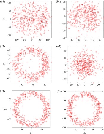
Figure 11. (a) PIV POD and (b) PLIF POD coefficients for the first two modes plotted against each other. POD analysis extracted from instantaneous centreplane (side view) simultaneous PLIF/PIV imaging of the
 $S=1.00$
, flush nozzle-generated JICF with varying momentum flux ratios:
$S=1.00$
, flush nozzle-generated JICF with varying momentum flux ratios:
 $J=41$
(a1,b1),
$J=41$
(a1,b1),
 $J=12$
(a2,b2), and
$J=12$
(a2,b2), and
 $J=5$
(a3,b3).
$J=5$
(a3,b3).
It is worthwhile to explore the similarity between mode 1 and mode 2 for the data shown in figures 9 and 10. Following the work of Meyer et al. (Reference Meyer, Pedersen and Özcan2007), one can plot the POD coefficients of the first and second modes for all snapshots analysed. If the coefficients of the first two modes plotted against each other yields a circle, then the structure in question is a periodic travelling wave that is characterized by linear combinations of the two modes. Figures 11(a) and 11(b) plot the coefficients of the first two modes (
 $a_{1}$
and
$a_{1}$
and
 $a_{2}$
), extracted from the PIV and PLIF POD analyses, respectively, via figures 9 and 10. As expected, as the momentum flux ratio was lowered and the flow transitioned to absolute instability (as noted above, yielding strongly periodic upstream shear layer vortex roll up), the coefficients of the first two modes plotted against each other for the PIV-based POD began to form a circular shape. For
$a_{2}$
), extracted from the PIV and PLIF POD analyses, respectively, via figures 9 and 10. As expected, as the momentum flux ratio was lowered and the flow transitioned to absolute instability (as noted above, yielding strongly periodic upstream shear layer vortex roll up), the coefficients of the first two modes plotted against each other for the PIV-based POD began to form a circular shape. For
 $J=5$
, the coefficient plot showed strong periodicity for both PLIF and PIV POD analyses, suggesting that the upstream shear layer absolute instability dominated the evolution of both scalar and velocity fields for this flow condition. For clearly convectively unstable conditions, as for
$J=5$
, the coefficient plot showed strong periodicity for both PLIF and PIV POD analyses, suggesting that the upstream shear layer absolute instability dominated the evolution of both scalar and velocity fields for this flow condition. For clearly convectively unstable conditions, as for
 $J=41$
, the shear layer instabilities were weaker and broadband in nature, without strong downstream periodic convection, and this yielded a more random pattern in figure 11(a1,b1). While the periodicity was not apparent in the PLIF POD coefficient plot for
$J=41$
, the shear layer instabilities were weaker and broadband in nature, without strong downstream periodic convection, and this yielded a more random pattern in figure 11(a1,b1). While the periodicity was not apparent in the PLIF POD coefficient plot for
 $J=12$
(see figure 11
b2), this transitional flow condition did produce periodicity in the coefficients derived from the velocity data (figure 11
a2). While it was not expected that the
$J=12$
(see figure 11
b2), this transitional flow condition did produce periodicity in the coefficients derived from the velocity data (figure 11
a2). While it was not expected that the
 $J=12$
case would yield different results between PLIF- and PIV-based coefficients, clearly, as noted by Kothnur & Clemens (Reference Kothnur and Clemens2005), the velocity field and scalar field can respond differently to flow perturbations in a transitional flow, even for unity Schmidt number flows. This could be especially relevant here, in that the jet mixture for equidensity conditions with acetone produced a Schmidt number of 0.389 (table 1). As the JICF shear layer undergoes a transition in its nature, as occurs between
$J=12$
case would yield different results between PLIF- and PIV-based coefficients, clearly, as noted by Kothnur & Clemens (Reference Kothnur and Clemens2005), the velocity field and scalar field can respond differently to flow perturbations in a transitional flow, even for unity Schmidt number flows. This could be especially relevant here, in that the jet mixture for equidensity conditions with acetone produced a Schmidt number of 0.389 (table 1). As the JICF shear layer undergoes a transition in its nature, as occurs between
 $J=12$
and 5, even with acetone present (Shoji Reference Shoji2017), such differences in velocity and scalar response could become even more pronounced.
$J=12$
and 5, even with acetone present (Shoji Reference Shoji2017), such differences in velocity and scalar response could become even more pronounced.

Figure 12. PIV POD mode structures extracted from instantaneous centreplane (side view) simultaneous PLIF/PIV imaging of
 $S=0.35$
, flush nozzle-generated JICF with varying momentum flux ratios: (a)
$S=0.35$
, flush nozzle-generated JICF with varying momentum flux ratios: (a)
 $J=41$
, (b)
$J=41$
, (b)
 $J=12$
, (c)
$J=12$
, (c)
 $J=5$
. Data shown for mode 1 (a1–c1), mode 2 (a2–c2), mode 3 (a3–c3), mode 4 (a4–c4). Arrows in images indicate in-plane velocity component structure contribution, while colour map indicates out-of-plane velocity component structure contribution. Percentage of total velocity fluctuation energy (VE) contributed by each mode is indicated below each image. (The colour bar represents each mode scaled by its own norm and the mean jet velocity at the jet exit
$J=5$
. Data shown for mode 1 (a1–c1), mode 2 (a2–c2), mode 3 (a3–c3), mode 4 (a4–c4). Arrows in images indicate in-plane velocity component structure contribution, while colour map indicates out-of-plane velocity component structure contribution. Percentage of total velocity fluctuation energy (VE) contributed by each mode is indicated below each image. (The colour bar represents each mode scaled by its own norm and the mean jet velocity at the jet exit
 $U_{j}$
.)
$U_{j}$
.)

Figure 13. PLIF POD mode structures extracted from instantaneous centreplane (side view) simultaneous PLIF/PIV imaging of
 $S=0.35$
, flush nozzle-generated JICF with varying momentum flux ratios: (a)
$S=0.35$
, flush nozzle-generated JICF with varying momentum flux ratios: (a)
 $J=41$
, (b)
$J=41$
, (b)
 $J=12$
, (c)
$J=12$
, (c)
 $J=5$
. Data shown for mode 1 (a1–c1), mode 2 (a2–c2), mode 3 (a3–c3), mode 4 (a4–c4). Percentage of total scalar fluctuation energy (SE) contributed by each mode is indicated below each image. (The colour bar represents each mode scaled by its own norm and the mean jet velocity at the jet exit
$J=5$
. Data shown for mode 1 (a1–c1), mode 2 (a2–c2), mode 3 (a3–c3), mode 4 (a4–c4). Percentage of total scalar fluctuation energy (SE) contributed by each mode is indicated below each image. (The colour bar represents each mode scaled by its own norm and the mean jet velocity at the jet exit
 $U_{j}$
.)
$U_{j}$
.)
Figures 12 and 13 show visualizations of the first four modes extracted from the PIV and PLIF POD analyses applied to the
 $S=0.35$
, flush nozzle-injected transverse jets for
$S=0.35$
, flush nozzle-injected transverse jets for
 $J=41$
,
$J=41$
,
 $J=12$
and
$J=12$
and
 $J=5$
, which all involved absolutely unstable upstream shear layers (Getsinger et al.
Reference Getsinger, Gevorkyan, Smith and Karagozian2014). Compared to the equidensity modes in figures 9 and 10, the PIV and PLIF POD modes for the
$J=5$
, which all involved absolutely unstable upstream shear layers (Getsinger et al.
Reference Getsinger, Gevorkyan, Smith and Karagozian2014). Compared to the equidensity modes in figures 9 and 10, the PIV and PLIF POD modes for the
 $S=0.35$
case shown in figures 12 and 13 had somewhat more chaotic and irregular-appearing structures. It is worthwhile to note that although the first two
$S=0.35$
case shown in figures 12 and 13 had somewhat more chaotic and irregular-appearing structures. It is worthwhile to note that although the first two
 $S=0.35$
, PIV POD modes for
$S=0.35$
, PIV POD modes for
 $J=41$
were clearly shear layer modes (first and second rows of figure 12
a), the first two PLIF POD modes were actually associated with structures on the lee side of the jet (first and second row of figure 13
a). Thus, the lee-side jet stabilities of the
$J=41$
were clearly shear layer modes (first and second rows of figure 12
a), the first two PLIF POD modes were actually associated with structures on the lee side of the jet (first and second row of figure 13
a). Thus, the lee-side jet stabilities of the
 $S=0.35$
,
$S=0.35$
,
 $J=41$
jet had a more significant impact on the scalar field distribution and fluctuation content than on the velocity field. As the momentum flux ratio
$J=41$
jet had a more significant impact on the scalar field distribution and fluctuation content than on the velocity field. As the momentum flux ratio
 $J$
was lowered for
$J$
was lowered for
 $S=0.35$
, the first two PLIF POD modes transitioned to becoming shear layer modes (e.g. compare
$S=0.35$
, the first two PLIF POD modes transitioned to becoming shear layer modes (e.g. compare
 $J=41$
to
$J=41$
to
 $J=5$
in figure 13). This transition from lee-side instability dominance to upstream shear layer behaviour dominance in the scalar field for these low density jets could in part be responsible for the reduction in mixing observed when one lowers
$J=5$
in figure 13). This transition from lee-side instability dominance to upstream shear layer behaviour dominance in the scalar field for these low density jets could in part be responsible for the reduction in mixing observed when one lowers
 $J$
at a fixed density ratio below the critical value of
$J$
at a fixed density ratio below the critical value of
 $S\cong 0.40$
, although differences in cross-flow entrainment into variable density vortical structures are also important (Gevorkyan et al.
Reference Gevorkyan, Shoji, Getsinger, Smith and Karagozian2016).
$S\cong 0.40$
, although differences in cross-flow entrainment into variable density vortical structures are also important (Gevorkyan et al.
Reference Gevorkyan, Shoji, Getsinger, Smith and Karagozian2016).

Figure 14. (a) PIV POD and (b) PLIF POD coefficients for the first two modes plotted against each other. POD analysis extracted from instantaneous centreplane (side view) simultaneous PLIF/PIV imaging of the
 $S=0.35$
, flush nozzle-generated JICF with varying momentum flux ratios:
$S=0.35$
, flush nozzle-generated JICF with varying momentum flux ratios:
 $J=41$
(a1,b1),
$J=41$
(a1,b1),
 $J=12$
(a2,b2),
$J=12$
(a2,b2),
 $J=5$
(a3,b3).
$J=5$
(a3,b3).
The first and second mode coefficients for these
 $S=0.35$
jets, shown in figure 14, showed strong periodicity in the upstream shear layer for PIV-based POD at
$S=0.35$
jets, shown in figure 14, showed strong periodicity in the upstream shear layer for PIV-based POD at
 $J=41$
, but with greater irregularity as momentum flux ratio was reduced, even though such a reduction in
$J=41$
, but with greater irregularity as momentum flux ratio was reduced, even though such a reduction in
 $J$
still produced an absolutely unstable upstream shear layer. Clearly, the differences in the dynamics captured by the velocity and scalar fields in a variable density flow affected the relative energy content in the modes and their relationships that would suggest travelling wave behaviour. Yet it was apparent that the first two modes for
$J$
still produced an absolutely unstable upstream shear layer. Clearly, the differences in the dynamics captured by the velocity and scalar fields in a variable density flow affected the relative energy content in the modes and their relationships that would suggest travelling wave behaviour. Yet it was apparent that the first two modes for
 $J=12$
and
$J=12$
and
 $J=5$
in figures 12(b) and 12(c) contained significant kinetic energy in wake vortices as well as shear layer vortices. These observations also could be related to the altered nature of cross-flow entrainment by upstream shear layer vortices for the low density JICF with a reduction in
$J=5$
in figures 12(b) and 12(c) contained significant kinetic energy in wake vortices as well as shear layer vortices. These observations also could be related to the altered nature of cross-flow entrainment by upstream shear layer vortices for the low density JICF with a reduction in
 $J$
, as documented in Gevorkyan et al. (Reference Gevorkyan, Shoji, Getsinger, Smith and Karagozian2016).
$J$
, as documented in Gevorkyan et al. (Reference Gevorkyan, Shoji, Getsinger, Smith and Karagozian2016).

Figure 15. PIV POD mode structures extracted from instantaneous centreplane (side view) simultaneous PLIF/PIV imaging of
 $S=1.00$
, flush pipe-generated JICF with varying momentum flux ratios: (a)
$S=1.00$
, flush pipe-generated JICF with varying momentum flux ratios: (a)
 $J=41$
, (b)
$J=41$
, (b)
 $J=12$
, (c)
$J=12$
, (c)
 $J=5$
. Data shown for mode 1 (a1–c1), mode 2 (a2–c2), mode 3 (a3–c3), mode 4 (a4–c4). Arrows in images indicate in-plane velocity component structure contribution, while colour map indicates out-of-plane velocity component structure contribution. Percentage of total kinetic energy (KE) contributed by each mode is indicated below each image. (The colour bar represents each mode scaled by its own norm and the mean jet velocity at the jet exit
$J=5$
. Data shown for mode 1 (a1–c1), mode 2 (a2–c2), mode 3 (a3–c3), mode 4 (a4–c4). Arrows in images indicate in-plane velocity component structure contribution, while colour map indicates out-of-plane velocity component structure contribution. Percentage of total kinetic energy (KE) contributed by each mode is indicated below each image. (The colour bar represents each mode scaled by its own norm and the mean jet velocity at the jet exit
 $U_{j}$
.)
$U_{j}$
.)

Figure 16. PLIF POD mode structures extracted from instantaneous centreplane (side view) simultaneous PLIF/PIV imaging of
 $S=1.00$
, flush pipe-generated JICF with varying momentum flux ratios: (a)
$S=1.00$
, flush pipe-generated JICF with varying momentum flux ratios: (a)
 $J=41$
, (b)
$J=41$
, (b)
 $J=12$
, (c)
$J=12$
, (c)
 $J=5$
. Data shown for mode 1 (a1–c1), mode 2 (a2–c2), mode 3 (a3–c3), mode 4 (a4–c4). Percentage of total scalar fluctuation energy (SE) contributed by each mode is indicated below each image. (The colour bar represents each mode scaled by its own norm and the mean jet velocity at the jet exit
$J=5$
. Data shown for mode 1 (a1–c1), mode 2 (a2–c2), mode 3 (a3–c3), mode 4 (a4–c4). Percentage of total scalar fluctuation energy (SE) contributed by each mode is indicated below each image. (The colour bar represents each mode scaled by its own norm and the mean jet velocity at the jet exit
 $U_{j}$
.)
$U_{j}$
.)
Figures 15 and 16 show visualizations of the first four modes extracted from the PIV POD and PLIF POD analyses, respectively, for the equidensity, flush pipe-injected transverse jets at
 $J=41$
,
$J=41$
,
 $J=12$
and
$J=12$
and
 $J=5$
, extracted from data such as those in figure 8. Similar to the modes for the equidensity flush nozzle cases shown in figures 9 and 10, the first two PLIF and PIV POD modes for the flush pipe-injected jets shown in figures 15 and 16 were composed primarily of shear layer structures, although they were comparatively weaker than for the nozzle-generated jets. Also as seen for the equidensity flush nozzle-injected jets, the first and second mode coefficients for the flush pipe-injected jets, shown in figure 17, demonstrated increasing periodicity as
$J=5$
, extracted from data such as those in figure 8. Similar to the modes for the equidensity flush nozzle cases shown in figures 9 and 10, the first two PLIF and PIV POD modes for the flush pipe-injected jets shown in figures 15 and 16 were composed primarily of shear layer structures, although they were comparatively weaker than for the nozzle-generated jets. Also as seen for the equidensity flush nozzle-injected jets, the first and second mode coefficients for the flush pipe-injected jets, shown in figure 17, demonstrated increasing periodicity as
 $J$
was reduced and the upstream shear layer transitioned to becoming absolutely unstable for
$J$
was reduced and the upstream shear layer transitioned to becoming absolutely unstable for
 $J=5$
. As also seen in hotwire spectral measurements without acetone seeding (Getsinger et al.
Reference Getsinger, Gevorkyan, Smith and Karagozian2014), the transition to strong periodic behaviour as
$J=5$
. As also seen in hotwire spectral measurements without acetone seeding (Getsinger et al.
Reference Getsinger, Gevorkyan, Smith and Karagozian2014), the transition to strong periodic behaviour as
 $J$
was reduced from
$J$
was reduced from
 $J=12$
to
$J=12$
to
 $J=5$
was more abrupt for the flush pipe than for the flush nozzle.
$J=5$
was more abrupt for the flush pipe than for the flush nozzle.

Figure 17. (a) PIV POD and (b) PLIF POD coefficients for the first two modes plotted against each other. POD analysis extracted from instantaneous centreplane (side view) simultaneous PLIF/PIV imaging of the
 $S=1.00$
, flush pipe-generated JICF with varying momentum flux ratios:
$S=1.00$
, flush pipe-generated JICF with varying momentum flux ratios:
 $J=41$
(a1,b1),
$J=41$
(a1,b1),
 $J=12$
(a2,b2), and
$J=12$
(a2,b2), and
 $J=5$
(a3,b3).
$J=5$
(a3,b3).
3.3 Scalar dissipation rates and strain rates
As outlined in § 1.2, there is a direct link between the underlying strain field of any fluid flow where mixing of dissimilar fluids is taking place and the scalar gradient field that facilitates mixing (Peters Reference Peters1986). In this section, that link will be explored in detail by comparing the strain field
 $\unicode[STIX]{x1D716}$
acting along the JICF shear layers, as defined in (1.1), and quantified via PIV, to the local scalar dissipation rate field
$\unicode[STIX]{x1D716}$
acting along the JICF shear layers, as defined in (1.1), and quantified via PIV, to the local scalar dissipation rate field
 $\unicode[STIX]{x1D712}$
, as defined in (1.2) and quantified via acetone PLIF imaging. It should be noted, however, that the simultaneous PLIF/PIV measurements in this study only yielded two-dimensional strain rate/scalar dissipation rate data. Hence, possible variations in the third dimension should be taken into account when interpreting results. Measurement noise, e.g. shot noise, camera noise, background fluctuations, etc., could also have an effect on gradients calculated from the PLIF and PIV data. In order to reduce the effect of noise on the results, aside from the various filters applied to both the PLIF and PIV data, all gradient quantities calculated were averaged over each set of images.
$\unicode[STIX]{x1D712}$
, as defined in (1.2) and quantified via acetone PLIF imaging. It should be noted, however, that the simultaneous PLIF/PIV measurements in this study only yielded two-dimensional strain rate/scalar dissipation rate data. Hence, possible variations in the third dimension should be taken into account when interpreting results. Measurement noise, e.g. shot noise, camera noise, background fluctuations, etc., could also have an effect on gradients calculated from the PLIF and PIV data. In order to reduce the effect of noise on the results, aside from the various filters applied to both the PLIF and PIV data, all gradient quantities calculated were averaged over each set of images.
3.3.1 Shear layer determination
In order to compare the velocity and scalar gradient quantities utilizing simultaneous acetone PLIF and stereo PIV measurements, a method for determining the location of the dominant upstream and downstream shear layers between jet and cross-flow fluid was developed. Utilizing the mean jet trajectory based on concentration maxima from the PLIF data, a transformation from the
 $x{-}z$
coordinate system (shown in figure 1) to the
$x{-}z$
coordinate system (shown in figure 1) to the
 $s_{c}-n$
(centreline jet normal) coordinate system was implemented, similar to the method utilized for JICF mixing studies (see Gevorkyan et al. (Reference Gevorkyan, Shoji, Getsinger, Smith and Karagozian2016) for details on the transformation method). After the transformation was implemented, the shear layer location was determined as the locus with the maximum scalar dissipation rate along a ray normal to each
$s_{c}-n$
(centreline jet normal) coordinate system was implemented, similar to the method utilized for JICF mixing studies (see Gevorkyan et al. (Reference Gevorkyan, Shoji, Getsinger, Smith and Karagozian2016) for details on the transformation method). After the transformation was implemented, the shear layer location was determined as the locus with the maximum scalar dissipation rate along a ray normal to each
 $s_{c}/D$
position. This analysis yielded the local shear layer coordinate
$s_{c}/D$
position. This analysis yielded the local shear layer coordinate
 $s_{l}$
and its local layer-normal direction
$s_{l}$
and its local layer-normal direction
 $n_{l}$
. An average shear layer trajectory coordinate
$n_{l}$
. An average shear layer trajectory coordinate
 $s$
, used in prior JICF instability studies (Megerian et al.
Reference Megerian, Davitian, de B. Alves and Karagozian2007; Davitian et al.
Reference Davitian, Getsinger, Hendrickson and Karagozian2010a
) is shown in figure 1. A similar method was utilized to track the downstream (lee-side) shear layer location. All average scalar dissipation rates and strain rates shown in this study were calculated at the instantaneous shear/mixing layer location determined from this method, and then averaged over the set of images for the coordinate location
$s$
, used in prior JICF instability studies (Megerian et al.
Reference Megerian, Davitian, de B. Alves and Karagozian2007; Davitian et al.
Reference Davitian, Getsinger, Hendrickson and Karagozian2010a
) is shown in figure 1. A similar method was utilized to track the downstream (lee-side) shear layer location. All average scalar dissipation rates and strain rates shown in this study were calculated at the instantaneous shear/mixing layer location determined from this method, and then averaged over the set of images for the coordinate location
 $s_{c}$
.
$s_{c}$
.
3.3.2 Maximum scalar dissipation rate and minimum principal strain rate
As noted previously, scalar mixing structures in turbulent flows tend to exhibit a layer-like topology, with the scalar gradient direction aligned with the minimum principal (compressive) strain axis. Invoking this approximation of the underlying physics (Peters Reference Peters1986) for mixing layers in the present JICF study, one can compare scalar dissipation rates calculated from the PLIF measurements to the minimum principal strain rates calculated from the simultaneous PIV data at the same location to see if there were correlations among the trends. This comparison was administered for both the upstream and downstream mixing layers of equidensity flush nozzle- and flush pipe-injected transverse jets at the same momentum flux ratios.
 $\unicode[STIX]{x1D712}$
was determined via (1.2) from PLIF scalar data, utilizing the binary diffusivities for the acetone–gas jet mixtures into air as relevant for
$\unicode[STIX]{x1D712}$
was determined via (1.2) from PLIF scalar data, utilizing the binary diffusivities for the acetone–gas jet mixtures into air as relevant for
 $S=1.00$
and
$S=1.00$
and
 $S=0.35$
conditions, given in table 1. One could argue that the diffusion of acetone alone into air might be appropriate for incorporation in (1.2) because it is acetone fluorescence intensity that is quantified in PLIF imaging (Kothnur & Clemens Reference Kothnur and Clemens2005). But because it is the mixture of acetone and jet fluid that contains the particles incorporated in PIV-based quantification of strain rate, and because this mixture is what actually diffuses into air, especially in the relative near field of the jet, in the present studies we utilized the diffusivities for acetone mixtures shown in table 1 for evaluation of scalar dissipation rates via (1.2).
$S=0.35$
conditions, given in table 1. One could argue that the diffusion of acetone alone into air might be appropriate for incorporation in (1.2) because it is acetone fluorescence intensity that is quantified in PLIF imaging (Kothnur & Clemens Reference Kothnur and Clemens2005). But because it is the mixture of acetone and jet fluid that contains the particles incorporated in PIV-based quantification of strain rate, and because this mixture is what actually diffuses into air, especially in the relative near field of the jet, in the present studies we utilized the diffusivities for acetone mixtures shown in table 1 for evaluation of scalar dissipation rates via (1.2).
The magnitude of the minimum principal (compressive) strain rate
 $\unicode[STIX]{x1D716}_{min}$
was determined from PIV data by taking the absolute value of the negative strain rate extracted from the diagonalized strain rate tensor shown in (1.1), which consists of two strain rate components with opposite signs. This minimum principal compressive strain rate value was then averaged at the local shear layer location over 500 image sets.
$\unicode[STIX]{x1D716}_{min}$
was determined from PIV data by taking the absolute value of the negative strain rate extracted from the diagonalized strain rate tensor shown in (1.1), which consists of two strain rate components with opposite signs. This minimum principal compressive strain rate value was then averaged at the local shear layer location over 500 image sets.
Trends in the variation in average scalar dissipation rate
 $\overline{\unicode[STIX]{x1D712}}$
and minimum principal strain rate
$\overline{\unicode[STIX]{x1D712}}$
and minimum principal strain rate
 $\overline{\unicode[STIX]{x1D716}}_{min}$
along the upstream and downstream mixing layers for the equidensity flush nozzle-injected and flush pipe-injected transverse jets showed similar general behaviour as a function of
$\overline{\unicode[STIX]{x1D716}}_{min}$
along the upstream and downstream mixing layers for the equidensity flush nozzle-injected and flush pipe-injected transverse jets showed similar general behaviour as a function of
 $s_{c}/D$
(Gevorkyan Reference Gevorkyan2015), but with notable differences, especially in the jet’s near field. Such differences suggest that the minimum principal axis did not necessarily align with the scalar gradient vector. Figure 18 highlights the magnitude of the average angle difference,
$s_{c}/D$
(Gevorkyan Reference Gevorkyan2015), but with notable differences, especially in the jet’s near field. Such differences suggest that the minimum principal axis did not necessarily align with the scalar gradient vector. Figure 18 highlights the magnitude of the average angle difference,
 $|\unicode[STIX]{x1D6FC}|$
, between the minimum principal axis of strain determined from the PIV data and the scalar gradient vector direction from the PLIF data for the different injector flows. Angle difference data are shown for both the upstream shear or mixing layer (UML) and downstream or lee-side mixing layer (DML). If there were perfect alignment between the minimum principal axis of strain and the scalar gradient vector direction, as in a flow field of pure straining, the average angle difference would be zero along the jet trajectory (Kothnur & Clemens Reference Kothnur and Clemens2005).
$|\unicode[STIX]{x1D6FC}|$
, between the minimum principal axis of strain determined from the PIV data and the scalar gradient vector direction from the PLIF data for the different injector flows. Angle difference data are shown for both the upstream shear or mixing layer (UML) and downstream or lee-side mixing layer (DML). If there were perfect alignment between the minimum principal axis of strain and the scalar gradient vector direction, as in a flow field of pure straining, the average angle difference would be zero along the jet trajectory (Kothnur & Clemens Reference Kothnur and Clemens2005).
Figure 18. Magnitude of average angle difference,
 $|\unicode[STIX]{x1D6FC}|$
, between the minimum principal compressive strain axis and the maximum scalar gradient vector. Data shown for both the upstream mixing layer (UML) and downstream mixing layer (DML) of flush nozzle-injected and flush pipe-injected,
$|\unicode[STIX]{x1D6FC}|$
, between the minimum principal compressive strain axis and the maximum scalar gradient vector. Data shown for both the upstream mixing layer (UML) and downstream mixing layer (DML) of flush nozzle-injected and flush pipe-injected,
 $S=1.00$
transverse jets with (a)
$S=1.00$
transverse jets with (a)
 $J=41$
, (b)
$J=41$
, (b)
 $J=12$
, and (c)
$J=12$
, and (c)
 $J=5$
.
$J=5$
.
The results in figure 18 are similar to what one would expect for this relatively low Reynolds number, transitional transverse jet. Near the jet exit, before shear layer-generated vortex formation for the
 $J=41$
transverse jets occurred (for either injector), the magnitude of the angle difference was close to
$J=41$
transverse jets occurred (for either injector), the magnitude of the angle difference was close to
 $45^{\circ }$
, as expected for a shear-dominant environment. For the upstream shear layer, initial vortex formation caused a drop in the angle difference, for example, as in the flush nozzle,
$45^{\circ }$
, as expected for a shear-dominant environment. For the upstream shear layer, initial vortex formation caused a drop in the angle difference, for example, as in the flush nozzle,
 $J=41$
UML angle difference data in figure 18(a) at
$J=41$
UML angle difference data in figure 18(a) at
 $s_{c}/D\approx 2.5$
, or in the flush nozzle,
$s_{c}/D\approx 2.5$
, or in the flush nozzle,
 $J=12$
UML data in figure 18(b) at
$J=12$
UML data in figure 18(b) at
 $s_{c}/D\approx 1.5$
. This correspondence to initial vortex roll-up location may be understood via comparison with
$s_{c}/D\approx 1.5$
. This correspondence to initial vortex roll-up location may be understood via comparison with
 $J=41$
and
$J=41$
and
 $12$
images in figure 6. Figure 18 highlights the fact that the angle difference between the maximum scalar gradient vector and the minimum principal strain axis was rarely close to zero, except during the initial vortex roll up associated with the absolutely unstable
$12$
images in figure 6. Figure 18 highlights the fact that the angle difference between the maximum scalar gradient vector and the minimum principal strain axis was rarely close to zero, except during the initial vortex roll up associated with the absolutely unstable
 $J=5$
upstream shear layer for the flush nozzle (figure 18
c), consistent with strong local straining. In general, then, a quantitative comparison of the local scalar dissipation rate to the component of strain along the scalar gradient vector direction would be a more appropriate comparison to make here, especially given the relevance of the former to reactive interfaces (Bish & Dahm Reference Bish and Dahm1995). Hence, for quantitative comparisons with both PLIF-extracted scalar dissipation rate and strain rates, the PIV-extracted strain rate was determined in the direction of the local scalar gradient, as described below.
$J=5$
upstream shear layer for the flush nozzle (figure 18
c), consistent with strong local straining. In general, then, a quantitative comparison of the local scalar dissipation rate to the component of strain along the scalar gradient vector direction would be a more appropriate comparison to make here, especially given the relevance of the former to reactive interfaces (Bish & Dahm Reference Bish and Dahm1995). Hence, for quantitative comparisons with both PLIF-extracted scalar dissipation rate and strain rates, the PIV-extracted strain rate was determined in the direction of the local scalar gradient, as described below.
3.3.3 Maximum scalar dissipation rate and layer-normal strain rate
One can make a direct comparison of the scalar dissipation rate to the strain rate in the scalar gradient direction, neglecting three-dimensional effects, as noted previously. This evaluation in the
 $y=0$
plane assumes that compressive strain normal to a scalar dissipation layer dominates the evolution of the scalar dissipation rate. Such comparison could yield insights into JICF evolution, mixing, and, indirectly, reaction characteristics. Note that in the absence of time-resolved data, the comparison between the scalar dissipation rate and strain rate is only valid when the strain rate normal to the layer is compressive, since a quasi-steady state solution to the advection–diffusion equation of the scalar is only possible when the molecular diffusion in the scalar gradient direction is balanced by compressive strain in the scalar gradient direction and extensive strain along the layer normal to the scalar gradient direction (Bish & Dahm Reference Bish and Dahm1995). If there is extensive strain in the scalar gradient direction, both strain and diffusion act to decrease the scalar dissipation rate and a quasi-steady solution to the advection–diffusion equation is not possible. Hence, in order to compare the trends among scalar dissipation rates and strain rates, any PLIF- or PIV-extracted strain rates that were negative, thus with extensive strain in the scalar gradient direction, were removed from the averaging process via an automated check. As found in the study of Kothnur & Clemens (Reference Kothnur and Clemens2005) for transitional and turbulent planar jets, extensive strain normal to the scalar gradient direction was found for the JICF to affect the evolution of scalar structures quite often, especially in regions immediately preceding vortex roll up (e.g.
$y=0$
plane assumes that compressive strain normal to a scalar dissipation layer dominates the evolution of the scalar dissipation rate. Such comparison could yield insights into JICF evolution, mixing, and, indirectly, reaction characteristics. Note that in the absence of time-resolved data, the comparison between the scalar dissipation rate and strain rate is only valid when the strain rate normal to the layer is compressive, since a quasi-steady state solution to the advection–diffusion equation of the scalar is only possible when the molecular diffusion in the scalar gradient direction is balanced by compressive strain in the scalar gradient direction and extensive strain along the layer normal to the scalar gradient direction (Bish & Dahm Reference Bish and Dahm1995). If there is extensive strain in the scalar gradient direction, both strain and diffusion act to decrease the scalar dissipation rate and a quasi-steady solution to the advection–diffusion equation is not possible. Hence, in order to compare the trends among scalar dissipation rates and strain rates, any PLIF- or PIV-extracted strain rates that were negative, thus with extensive strain in the scalar gradient direction, were removed from the averaging process via an automated check. As found in the study of Kothnur & Clemens (Reference Kothnur and Clemens2005) for transitional and turbulent planar jets, extensive strain normal to the scalar gradient direction was found for the JICF to affect the evolution of scalar structures quite often, especially in regions immediately preceding vortex roll up (e.g.
 $z/D\approx 2.1$
for the equidensity flush nozzle-injected
$z/D\approx 2.1$
for the equidensity flush nozzle-injected
 $J=41$
jet, as shown in figure 6
a1,b1). In order to ensure statistical significance, a qualifier was applied to the averaging process that required at least 200 data points to be contained within the averaging of layer-normal strain rate
$J=41$
jet, as shown in figure 6
a1,b1). In order to ensure statistical significance, a qualifier was applied to the averaging process that required at least 200 data points to be contained within the averaging of layer-normal strain rate
 $\overline{\unicode[STIX]{x1D716}}$
and scalar dissipation rate
$\overline{\unicode[STIX]{x1D716}}$
and scalar dissipation rate
 $\overline{\unicode[STIX]{x1D712}}$
at each
$\overline{\unicode[STIX]{x1D712}}$
at each
 $s_{c}/D$
location.
$s_{c}/D$
location.

Figure 19. Mixing layer average maximum scalar dissipation rate (——, black),
 $\overline{\unicode[STIX]{x1D712}}$
and average strain rate normal to the scalar gradient direction (——, red),
$\overline{\unicode[STIX]{x1D712}}$
and average strain rate normal to the scalar gradient direction (——, red),
 $\overline{\unicode[STIX]{x1D716}}$
, of
$\overline{\unicode[STIX]{x1D716}}$
, of
 $S=1.00$
, flush nozzle-injected transverse jets with
$S=1.00$
, flush nozzle-injected transverse jets with
 $J=41$
(a1,b1),
$J=41$
(a1,b1),
 $J=12$
(a2,b2) and
$J=12$
(a2,b2) and
 $J=5$
(a3,b3). Data shown for (a) upstream mixing layer and (b) downstream mixing layer. Data points with extensive strain in the scalar gradient direction are removed from averaging process.
$J=5$
(a3,b3). Data shown for (a) upstream mixing layer and (b) downstream mixing layer. Data points with extensive strain in the scalar gradient direction are removed from averaging process.
Figure 19 compares the trends for upstream and downstream mixing layer average scalar dissipation rates
 $\overline{\unicode[STIX]{x1D712}}$
and average layer-normal strain rates
$\overline{\unicode[STIX]{x1D712}}$
and average layer-normal strain rates
 $\overline{\unicode[STIX]{x1D716}}$
for the flush nozzle-injected, equidensity transverse jets at
$\overline{\unicode[STIX]{x1D716}}$
for the flush nozzle-injected, equidensity transverse jets at
 $J=41$
, 12, and 5. The spatial evolution of the upstream mixing layer PLIF-extracted scalar dissipation rates and PIV-extracted strain rates (figure 19
a) generally corresponded well to one another for all
$J=41$
, 12, and 5. The spatial evolution of the upstream mixing layer PLIF-extracted scalar dissipation rates and PIV-extracted strain rates (figure 19
a) generally corresponded well to one another for all
 $J$
values when each parameter was determined along the scalar gradient vector direction. It is important to note that increases in strain rate and scalar dissipation rate were highly correlated in regions of initial upstream shear layer vortex roll up (e.g.
$J$
values when each parameter was determined along the scalar gradient vector direction. It is important to note that increases in strain rate and scalar dissipation rate were highly correlated in regions of initial upstream shear layer vortex roll up (e.g.
 $s_{c}/D\approx 2.7$
for
$s_{c}/D\approx 2.7$
for
 $J=41$
). The downstream mixing layer comparison for the evolution of scalar dissipation rate and layer-normal strain rate (figure 19
b) only showed correspondence for
$J=41$
). The downstream mixing layer comparison for the evolution of scalar dissipation rate and layer-normal strain rate (figure 19
b) only showed correspondence for
 $J=12$
, and little similarity for other conditions, likely arising from three-dimensional and/or highly transient effects in the wake region of the JICF. In figure 20, the flush pipe’s scalar dissipation rate and layer-normal strain rate trends for the same values of
$J=12$
, and little similarity for other conditions, likely arising from three-dimensional and/or highly transient effects in the wake region of the JICF. In figure 20, the flush pipe’s scalar dissipation rate and layer-normal strain rate trends for the same values of
 $J$
similarly showed good correspondence in the upstream mixing layer (figure 20
a). For the downstream mixing layer region of the flush pipe-injected jets (figure 20
b) there was somewhat better correspondence between
$J$
similarly showed good correspondence in the upstream mixing layer (figure 20
a). For the downstream mixing layer region of the flush pipe-injected jets (figure 20
b) there was somewhat better correspondence between
 $\overline{\unicode[STIX]{x1D712}}$
and
$\overline{\unicode[STIX]{x1D712}}$
and
 $\overline{\unicode[STIX]{x1D716}}$
than for flush nozzle conditions, especially for general trends at
$\overline{\unicode[STIX]{x1D716}}$
than for flush nozzle conditions, especially for general trends at
 $J=41$
and
$J=41$
and
 $J=5$
. This same approach may be used to compare
$J=5$
. This same approach may be used to compare
 $\overline{\unicode[STIX]{x1D712}}$
and
$\overline{\unicode[STIX]{x1D712}}$
and
 $\overline{\unicode[STIX]{x1D716}}$
for the lower density (
$\overline{\unicode[STIX]{x1D716}}$
for the lower density (
 $S=0.35$
) JICF conditions. As for equidensity conditions, results in figure 21 similarly showed good correspondence between
$S=0.35$
) JICF conditions. As for equidensity conditions, results in figure 21 similarly showed good correspondence between
 $\overline{\unicode[STIX]{x1D712}}$
and
$\overline{\unicode[STIX]{x1D712}}$
and
 $\overline{\unicode[STIX]{x1D716}}$
trends in the upstream layer, but poorer correspondence in the downstream shear/mixing layer, in fact, with opposing trends in spatial variation for
$\overline{\unicode[STIX]{x1D716}}$
trends in the upstream layer, but poorer correspondence in the downstream shear/mixing layer, in fact, with opposing trends in spatial variation for
 $J=5$
. Again, it is likely that these discrepancies for the DML were due to three-dimensional/transient effects, where interactions with wake vortices drawing fluid from the wall boundary layer into the jet had an increasingly important influence (Fric & Roshko Reference Fric and Roshko1994).
$J=5$
. Again, it is likely that these discrepancies for the DML were due to three-dimensional/transient effects, where interactions with wake vortices drawing fluid from the wall boundary layer into the jet had an increasingly important influence (Fric & Roshko Reference Fric and Roshko1994).

Figure 20. Mixing layer average maximum scalar dissipation rate (——, black),
 $\overline{\unicode[STIX]{x1D712}}$
and average strain rate normal to the scalar gradient direction (——, red),
$\overline{\unicode[STIX]{x1D712}}$
and average strain rate normal to the scalar gradient direction (——, red),
 $\overline{\unicode[STIX]{x1D716}}$
, of
$\overline{\unicode[STIX]{x1D716}}$
, of
 $S=1.00$
, flush pipe-injected transverse jets with
$S=1.00$
, flush pipe-injected transverse jets with
 $J=41$
(a1,b1),
$J=41$
(a1,b1),
 $J=12$
(a2,b2) and
$J=12$
(a2,b2) and
 $J=5$
(a3,b3). Data shown for (a) upstream mixing layer and (b) downstream mixing layer. Data points with extensive strain in the scalar gradient direction are removed from averaging process.
$J=5$
(a3,b3). Data shown for (a) upstream mixing layer and (b) downstream mixing layer. Data points with extensive strain in the scalar gradient direction are removed from averaging process.
Figure 21. Mixing layer average maximum scalar dissipation rate (——, black),
 $\overline{\unicode[STIX]{x1D712}}$
and average strain rate normal to the scalar gradient direction (——, red),
$\overline{\unicode[STIX]{x1D712}}$
and average strain rate normal to the scalar gradient direction (——, red),
 $\overline{\unicode[STIX]{x1D716}}$
, of
$\overline{\unicode[STIX]{x1D716}}$
, of
 $S=0.35$
, flush nozzle-injected transverse jets with
$S=0.35$
, flush nozzle-injected transverse jets with
 $J=41$
(a1,b1) and
$J=41$
(a1,b1) and
 $J=5$
(a2,b2). Data shown for (a) upstream mixing layer and (b) downstream mixing layer. Data points with extensive strain in the scalar gradient direction are removed from the averaging process.
$J=5$
(a2,b2). Data shown for (a) upstream mixing layer and (b) downstream mixing layer. Data points with extensive strain in the scalar gradient direction are removed from the averaging process.
3.3.4 Strained dissipation and reaction layer model applied to the JICF
In order to directly compare the strain rates extracted from the scalar field and from the velocity field in the JICF, the strained dissipation and reaction layer (SDRL) model (1.3) was employed (Bish & Dahm Reference Bish and Dahm1995); as noted earlier, the SDRL is based on classical flamelet models. This enabled the PLIF-based scalar data (and thus strain rate
 $\unicode[STIX]{x1D716}$
using (1.3)) to be compared directly to the strain rates extracted from the PIV-based velocity field data. The PLIF-based strain rate was calculated from scalar dissipation rates
$\unicode[STIX]{x1D716}$
using (1.3)) to be compared directly to the strain rates extracted from the PIV-based velocity field data. The PLIF-based strain rate was calculated from scalar dissipation rates
 $\overline{\unicode[STIX]{x1D712}}$
and scalar concentration measurements utilizing an automated method of error function fitting, formulated and applied to each instantaneous scalar mixing layer location; such fitting was required in order to determine the boundary scalar values
$\overline{\unicode[STIX]{x1D712}}$
and scalar concentration measurements utilizing an automated method of error function fitting, formulated and applied to each instantaneous scalar mixing layer location; such fitting was required in order to determine the boundary scalar values
 $\unicode[STIX]{x1D701}^{+}$
and
$\unicode[STIX]{x1D701}^{+}$
and
 $\unicode[STIX]{x1D701}^{-}$
in (1.3), which can have a significant influence on calculated strain rates. If one solves the one-dimensional scalar advection–diffusion equation, assuming quasi-steady behaviour and a locally uniform strain rate, the scalar distribution (normalized concentration
$\unicode[STIX]{x1D701}^{-}$
in (1.3), which can have a significant influence on calculated strain rates. If one solves the one-dimensional scalar advection–diffusion equation, assuming quasi-steady behaviour and a locally uniform strain rate, the scalar distribution (normalized concentration
 $C/C_{o}$
or
$C/C_{o}$
or
 $\unicode[STIX]{x1D701}$
) takes the form shown in (3.1):
$\unicode[STIX]{x1D701}$
) takes the form shown in (3.1):
 $$\begin{eqnarray}\unicode[STIX]{x1D701}=0.5(\unicode[STIX]{x1D701}^{+}+\unicode[STIX]{x1D701}-)+0.5(\unicode[STIX]{x1D701}^{+}-\unicode[STIX]{x1D701}-)\text{erf}(n_{l}/\unicode[STIX]{x1D706}_{D}).\end{eqnarray}$$
In this equation,
 $n_{l}$
is the layer-normal coordinate direction, which was assumed to be the two-dimensional scalar gradient direction determined from the PLIF measurements for each mixing layer location, and
$n_{l}$
is the layer-normal coordinate direction, which was assumed to be the two-dimensional scalar gradient direction determined from the PLIF measurements for each mixing layer location, and
 $\unicode[STIX]{x1D706}_{D}$
is the length scale that results from the competition between strain and diffusion (
$\unicode[STIX]{x1D706}_{D}$
is the length scale that results from the competition between strain and diffusion (
 $\unicode[STIX]{x1D706}_{D}=\sqrt{\hat{D}_{j\rightarrow \infty }/\unicode[STIX]{x1D716}}$
in the quasi-steady state limit, where
$\unicode[STIX]{x1D706}_{D}=\sqrt{\hat{D}_{j\rightarrow \infty }/\unicode[STIX]{x1D716}}$
in the quasi-steady state limit, where
 $\hat{D}$
is the binary diffusivity). In practice, an error function fit of the form shown in (3.2) was applied to the
$\hat{D}$
is the binary diffusivity). In practice, an error function fit of the form shown in (3.2) was applied to the
 $\unicode[STIX]{x1D701}=C/C_{o}$
data in the layer-normal direction
$\unicode[STIX]{x1D701}=C/C_{o}$
data in the layer-normal direction
 $n_{l}$
:
$n_{l}$
:
 $$\begin{eqnarray}\unicode[STIX]{x1D701}=a+b\times \text{erf}\left(\frac{n_{l}-c}{d}\right).\end{eqnarray}$$
The coefficient
 $c$
in (3.2) represents the offset of the fit from the centre location. The boundary conditions,
$c$
in (3.2) represents the offset of the fit from the centre location. The boundary conditions,
 $\unicode[STIX]{x1D701}^{+}=C/C_{o}^{+}$
and
$\unicode[STIX]{x1D701}^{+}=C/C_{o}^{+}$
and
 $\unicode[STIX]{x1D701}^{-}=C/C_{o}^{-}$
, were determined by comparing (3.1) to experimental concentration data. To ensure accuracy and applicability of the fit, besides requiring that the strain rate normal to the layer determined from comparative PIV data was compressive, another qualifier in the averaging process was applied based on the Pearson correlation coefficient of the fit (
$\unicode[STIX]{x1D701}^{-}=C/C_{o}^{-}$
, were determined by comparing (3.1) to experimental concentration data. To ensure accuracy and applicability of the fit, besides requiring that the strain rate normal to the layer determined from comparative PIV data was compressive, another qualifier in the averaging process was applied based on the Pearson correlation coefficient of the fit (
 $r>0.99$
). Additionally, error function fits assumed the magnitude of the coefficient
$r>0.99$
). Additionally, error function fits assumed the magnitude of the coefficient
 $|c|$
to be larger than the two-pixel width in PLIF images in order to have a more precise representation of the layer centre location; points outside of this criterion were removed from the strain rate evaluation. As with the data discussed in § 3.3.3, at least 200 data points for each
$|c|$
to be larger than the two-pixel width in PLIF images in order to have a more precise representation of the layer centre location; points outside of this criterion were removed from the strain rate evaluation. As with the data discussed in § 3.3.3, at least 200 data points for each
 $s_{c}/D$
location were required in the averaging process in order to consider the average to be statistically significant (Gevorkyan Reference Gevorkyan2015). An example fit for the flush nozzle-injected, equidensity
$s_{c}/D$
location were required in the averaging process in order to consider the average to be statistically significant (Gevorkyan Reference Gevorkyan2015). An example fit for the flush nozzle-injected, equidensity
 $J=5$
jet is shown in figure 22(a), utilizing the spatial resolution associated with PLIF data during simultaneous PLIF/PIV experiments. This fit to the error function is reasonably good.
$J=5$
jet is shown in figure 22(a), utilizing the spatial resolution associated with PLIF data during simultaneous PLIF/PIV experiments. This fit to the error function is reasonably good.

Figure 22. Example error function fits for flush-nozzle injected,
 $S=1.00$
,
$S=1.00$
,
 $J=5$
transverse jets. Data shown for (a) PLIF portion of simultaneous PLIF/PIV experiments and (b) high-resolution PLIF measurements.
$J=5$
transverse jets. Data shown for (a) PLIF portion of simultaneous PLIF/PIV experiments and (b) high-resolution PLIF measurements.

Figure 23. Average strain rate for the mixing layer calculated from PLIF-based scalar measurements using (1.3) (○) and average strain rate extracted from PIV in the direction normal to the scalar gradient direction (——, red), for the
 $S=1.00$
, flush nozzle-injected transverse jets with
$S=1.00$
, flush nozzle-injected transverse jets with
 $J=41$
(a1,b1),
$J=41$
(a1,b1),
 $J=12$
(a2,b2) and
$J=12$
(a2,b2) and
 $J=5$
(a3,b3). Data shown for (a) upstream mixing layer and (b) downstream mixing layer.
$J=5$
(a3,b3). Data shown for (a) upstream mixing layer and (b) downstream mixing layer.
Figure 23 compares the computed mixing layer strain rate calculated from the PLIF-based scalar measurements (3.1) to the average layer-normal strain rate extracted from the PIV measurements, for the equidensity flush nozzle-injected transverse jets at momentum flux ratios
 $J=41$
, 12, and 5. This comparison is administered for both upstream (figure 23
a) and downstream (figure 23
b) shear layers. For
$J=41$
, 12, and 5. This comparison is administered for both upstream (figure 23
a) and downstream (figure 23
b) shear layers. For
 $J=41$
, there was remarkable qualitative and quantitative correspondence between the PIV- and PLIF-based strain rates on both upstream and downstream mixing layers (figure 23
a1,b1), lending credence to the use of flamelet-like models for strained dissipation layers in non-reactive flows (Bish & Dahm Reference Bish and Dahm1995; Kothnur & Clemens Reference Kothnur and Clemens2005). There was similar correspondence between quantified increases in strain rates and general locations of initial shear layer vortex roll up for both the upstream and downstream layers observed in figures 6(a1) and 6(b1), respectively. As the momentum flux ratio was lowered to
$J=41$
, there was remarkable qualitative and quantitative correspondence between the PIV- and PLIF-based strain rates on both upstream and downstream mixing layers (figure 23
a1,b1), lending credence to the use of flamelet-like models for strained dissipation layers in non-reactive flows (Bish & Dahm Reference Bish and Dahm1995; Kothnur & Clemens Reference Kothnur and Clemens2005). There was similar correspondence between quantified increases in strain rates and general locations of initial shear layer vortex roll up for both the upstream and downstream layers observed in figures 6(a1) and 6(b1), respectively. As the momentum flux ratio was lowered to
 $J=12$
, the correlation between the PLIF- and PIV-based strain rate trends was also quite good in the UML but less so in the DML. In contrast, for
$J=12$
, the correlation between the PLIF- and PIV-based strain rate trends was also quite good in the UML but less so in the DML. In contrast, for
 $J=5$
in the near field of the UML, there were large PIV-based strain rates, consistent with strong vortex roll up taking place almost immediately, as indicated in figures 6(a3) and 6(b3). The corresponding spatial trends in PLIF-based strain rates were relatively poorly correlated with PIV-based data for
$J=5$
in the near field of the UML, there were large PIV-based strain rates, consistent with strong vortex roll up taking place almost immediately, as indicated in figures 6(a3) and 6(b3). The corresponding spatial trends in PLIF-based strain rates were relatively poorly correlated with PIV-based data for
 $J=5$
, although correlation with vortex roll up improved in the DML region, especially further downstream of injection. As expected, the upstream strain rates for the
$J=5$
, although correlation with vortex roll up improved in the DML region, especially further downstream of injection. As expected, the upstream strain rates for the
 $J=5$
absolutely unstable jet were considerably higher than those for convectively unstable
$J=5$
absolutely unstable jet were considerably higher than those for convectively unstable
 $J=41$
and
$J=41$
and
 $J=12$
jets. The separate determination that molecular mixing for the absolutely unstable JICF tends to be greater than that for the convectively unstable condition (described in detail in Gevorkyan et al. (Reference Gevorkyan, Shoji, Getsinger, Smith and Karagozian2016)) is consistent with the present strain rate estimates and spatial trends.
$J=12$
jets. The separate determination that molecular mixing for the absolutely unstable JICF tends to be greater than that for the convectively unstable condition (described in detail in Gevorkyan et al. (Reference Gevorkyan, Shoji, Getsinger, Smith and Karagozian2016)) is consistent with the present strain rate estimates and spatial trends.
It is difficult to definitively determine the exact cause of any qualitative and quantitative discrepancies for
 $J=12$
and 5 without time-resolved, fully three-dimensional measurements of the scalar and velocity fields. One explanation for the lack of correspondence on the downstream side of the jet for
$J=12$
and 5 without time-resolved, fully three-dimensional measurements of the scalar and velocity fields. One explanation for the lack of correspondence on the downstream side of the jet for
 $J=12$
, for example, could be associated with the superior ability of PIV to capture the evolving transient effects in the wake, on the lee side of the jet, as momentum flux ratio was lowered, as evidenced by the transient wake vortical structures in mode 3 and mode 4 observed to be present along with UML structures in the PIV POD for
$J=12$
, for example, could be associated with the superior ability of PIV to capture the evolving transient effects in the wake, on the lee side of the jet, as momentum flux ratio was lowered, as evidenced by the transient wake vortical structures in mode 3 and mode 4 observed to be present along with UML structures in the PIV POD for
 $J=12$
(third and fourth rows in figure 9
b). Another possible contributor to a lack of correspondence in trends for several cases studied here is the finite response time of the scalar dissipation layer to changes in actual strain rate. As summarized in the work of Kothnur & Clemens (Reference Kothnur and Clemens2005), the scalar dissipation layer response time is dependent on both amplitude and frequency of strain rate fluctuations, and it is also dependent on whether the strain rate is temporally increasing or decreasing. This could contribute to inaccuracies in PLIF-based strain rates. Spatial resolution may play an additional role here, and this will be explored below.
$J=12$
(third and fourth rows in figure 9
b). Another possible contributor to a lack of correspondence in trends for several cases studied here is the finite response time of the scalar dissipation layer to changes in actual strain rate. As summarized in the work of Kothnur & Clemens (Reference Kothnur and Clemens2005), the scalar dissipation layer response time is dependent on both amplitude and frequency of strain rate fluctuations, and it is also dependent on whether the strain rate is temporally increasing or decreasing. This could contribute to inaccuracies in PLIF-based strain rates. Spatial resolution may play an additional role here, and this will be explored below.

Figure 24. Average strain rate for the mixing layer calculated from PLIF-based scalar measurements using (1.3) (○) and average strain rate extracted from PIV in the direction normal to the scalar gradient direction (——, red), for the
 $S=1.00$
, flush pipe-injected transverse jets with
$S=1.00$
, flush pipe-injected transverse jets with
 $J=41$
(a1,b1),
$J=41$
(a1,b1),
 $J=12$
(a2,b2) and
$J=12$
(a2,b2) and
 $J=5$
(a3,b3). Data shown for (a) upstream mixing layer and (b) downstream mixing layer.
$J=5$
(a3,b3). Data shown for (a) upstream mixing layer and (b) downstream mixing layer.
Figure 24 shows the trends in upstream and downstream mixing layer PIV- and PLIF-based strain rates for the equidensity, flush pipe-injected transverse jets at
 $J=41$
, 12, and 5. As with the flush nozzle data in figure 23, the best correspondence in PLIF- and PIV-based strain rates for both UML and DML evolution in figure 24 was observed for convectively unstable conditions at
$J=41$
, 12, and 5. As with the flush nozzle data in figure 23, the best correspondence in PLIF- and PIV-based strain rates for both UML and DML evolution in figure 24 was observed for convectively unstable conditions at
 $J=41$
, with correspondence to delayed shear layer vorticity roll up as shown in figure 8, although correspondence for
$J=41$
, with correspondence to delayed shear layer vorticity roll up as shown in figure 8, although correspondence for
 $J=12$
was also reasonably good. Quantitative correspondence between the PLIF-calculated strain rate and the strain rate extracted from PIV was poorest for the absolutely unstable
$J=12$
was also reasonably good. Quantitative correspondence between the PLIF-calculated strain rate and the strain rate extracted from PIV was poorest for the absolutely unstable
 $J=5$
case in figure 24, despite similar qualitative trends to one another. Below we briefly explore the effects of PLIF spatial resolution as a possible culprit in the quantitative differences here, which appeared to be greatest for conditions of strong vorticity roll up and high strain rates, especially in the near field.
$J=5$
case in figure 24, despite similar qualitative trends to one another. Below we briefly explore the effects of PLIF spatial resolution as a possible culprit in the quantitative differences here, which appeared to be greatest for conditions of strong vorticity roll up and high strain rates, especially in the near field.
In determining the effect of spatial resolution on the quantitative comparisons of strain rates in figure 23, higher-resolution PLIF measurements previously used to study mixing processes in detail for the JICF (Gevorkyan et al.
Reference Gevorkyan, Shoji, Getsinger, Smith and Karagozian2016) were analysed using the methods outlined above. It should be noted that since no simultaneous PIV data could be taken with the higher-resolution PLIF data, mixing layer locations with extensional strain rate in the scalar gradient direction could not be removed from the averaging process, yielding uncertainty in the process of comparison. As noted earlier, the higher-resolution PLIF images had an in-plane resolution of
 $34~\unicode[STIX]{x03BC}\text{m}~\text{pixel}^{-1}$
, whereas the lower-resolution, PLIF portion of the simultaneous PLIF/PIV measurements, had an in-plane resolution of
$34~\unicode[STIX]{x03BC}\text{m}~\text{pixel}^{-1}$
, whereas the lower-resolution, PLIF portion of the simultaneous PLIF/PIV measurements, had an in-plane resolution of
 $65~\unicode[STIX]{x03BC}\text{m}~\text{pixel}^{-1}$
.
$65~\unicode[STIX]{x03BC}\text{m}~\text{pixel}^{-1}$
.
Scalar dissipation rates were determined per (1.2) for the data sets with two different resolutions. The effect of PLIF resolution on the strain rate is shown in figure 22(b) with an error function fit again used to evaluate the scalar boundary values
 $\unicode[STIX]{x1D701}^{+}$
and
$\unicode[STIX]{x1D701}^{+}$
and
 $\unicode[STIX]{x1D701}^{-}$
but now for PLIF data taken at higher resolution. There was a small yet noticeable improvement in the fit over the lower-resolution PLIF-PIV experiments, and this, in addition to the computation of
$\unicode[STIX]{x1D701}^{-}$
but now for PLIF data taken at higher resolution. There was a small yet noticeable improvement in the fit over the lower-resolution PLIF-PIV experiments, and this, in addition to the computation of
 $\overline{\unicode[STIX]{x1D712}}$
, altered the computed strain rates. The strain rates calculated from the error function fits of both high and lower-resolution PLIF data sets are shown in figure 25 for the UML of the equidensity flush nozzle-injected
$\overline{\unicode[STIX]{x1D712}}$
, altered the computed strain rates. The strain rates calculated from the error function fits of both high and lower-resolution PLIF data sets are shown in figure 25 for the UML of the equidensity flush nozzle-injected
 $J=41$
and
$J=41$
and
 $J=5$
transverse jets. Although general trends were not affected significantly by the differences in resolution for
$J=5$
transverse jets. Although general trends were not affected significantly by the differences in resolution for
 $J=41$
, the values of average local strain rate were significantly altered, with an increase in peak values of
$J=41$
, the values of average local strain rate were significantly altered, with an increase in peak values of
 $\overline{\unicode[STIX]{x1D716}}$
for
$\overline{\unicode[STIX]{x1D716}}$
for
 $J=41$
that in fact exceeded the magnitude of the PIV-derived strain rates for the UML in figure 23. For
$J=41$
that in fact exceeded the magnitude of the PIV-derived strain rates for the UML in figure 23. For
 $J=5$
, the higher resolution data also increased peak values of
$J=5$
, the higher resolution data also increased peak values of
 $\overline{\unicode[STIX]{x1D716}}$
, in this case bringing the PLIF-based strain rates into closer alignment, qualitatively and quantitatively, to the corresponding PIV-based data in figure 23.
$\overline{\unicode[STIX]{x1D716}}$
, in this case bringing the PLIF-based strain rates into closer alignment, qualitatively and quantitatively, to the corresponding PIV-based data in figure 23.
Figure 25. Average strain rate comparison between high-resolution PLIF imaging data (*, red) and PLIF portion of simultaneous PLIF/PIV measurements (○) for the upstream shear layer. Data shown for
 $S=1.00$
, flush nozzle-injected transverse jets with (a)
$S=1.00$
, flush nozzle-injected transverse jets with (a)
 $J=41$
and (b)
$J=41$
and (b)
 $J=5$
.
$J=5$
.
One may also correct in an approximate way for the effect of the PLIF measurement resolution on the strain rate calculation. An effective method for determining imaging system blur effects on the scalar gradients is outlined in the work of Wang & Clemens (Reference Wang and Clemens2004), where a line spread function (LSF) of the imaging system is determined using experimental data from a backlit razor blade traversed through the PLIF camera field of view. Using the LSF, one can determine the degradation of the scalar dissipation rate caused by the finite resolution of the entire imaging system (camera lens, intensifier and CCD array), and these were found to be very close to the resolution quantified by a target in the field of view, so the latter was most often used in the present analysis for simplicity. Calculation of the LSF was applied to the high-resolution PLIF images. The strain rates calculated from the images shown in figure 25 were corrected for the effect of imaging blur (Gevorkyan Reference Gevorkyan2015), and results for this correction are shown in figure 26, showing further increases in the peak values for
 $\overline{\unicode[STIX]{x1D716}}$
. After this strain rate correction was applied, the difference between the maximum strain rate calculated from the PLIF measurement for the flush nozzle-injected,
$\overline{\unicode[STIX]{x1D716}}$
. After this strain rate correction was applied, the difference between the maximum strain rate calculated from the PLIF measurement for the flush nozzle-injected,
 $J=5$
case, and the strain rate extracted from the PIV measurements for the same case (figure 23
a3) was reduced to 18 %, a remarkable correspondence considering all the factors that could affect this comparison beyond three-dimensional and transient effects, e.g. measurement noise, day-to-day-variations and PIV resolution and/or bias effects. Interestingly, the resolution-corrected PLIF-generated strain rates for
$J=5$
case, and the strain rate extracted from the PIV measurements for the same case (figure 23
a3) was reduced to 18 %, a remarkable correspondence considering all the factors that could affect this comparison beyond three-dimensional and transient effects, e.g. measurement noise, day-to-day-variations and PIV resolution and/or bias effects. Interestingly, the resolution-corrected PLIF-generated strain rates for
 $J=41$
in figure 26(a) were qualitatively similar to but significantly higher in magnitude than the PIV-extracted strain rate data for the same case shown in figure 23(a1). Given that extensional strain effects as well as deviation in angle between minimal principal compressive strain axis and maximum scalar gradient vector (figure 18
a) were rather significant for the
$J=41$
in figure 26(a) were qualitatively similar to but significantly higher in magnitude than the PIV-extracted strain rate data for the same case shown in figure 23(a1). Given that extensional strain effects as well as deviation in angle between minimal principal compressive strain axis and maximum scalar gradient vector (figure 18
a) were rather significant for the
 $J=41$
UML, one might expect somewhat poorer correspondence for these higher-resolution PLIF data, although clearly PIV resolution and other factors could be relevant to the differences observed here.
$J=41$
UML, one might expect somewhat poorer correspondence for these higher-resolution PLIF data, although clearly PIV resolution and other factors could be relevant to the differences observed here.

Figure 26. Resolution-corrected upstream shear layer strain rates calculated from high-resolution PLIF measurements. Data shown for
 $S=1.00$
, flush nozzle-injected transverse jets with (a)
$S=1.00$
, flush nozzle-injected transverse jets with (a)
 $J=41$
and (b)
$J=41$
and (b)
 $J=5$
. Raw strain rates (○) and resolution-corrected strain rates (*, red).
$J=5$
. Raw strain rates (○) and resolution-corrected strain rates (*, red).
3.3.5 Strain rates in lower density transverse jets
In this section, strain rates associated with upstream and downstream mixing layers at a lowered density ratio,
 $S=0.35$
for the flush nozzle-generated JICF, are discussed. For a non-unity density ratio in the flow field, a coordinate transformation is required to account for the density variation across the jet and cross-flow. The variation in density in the classical reaction–diffusion equation can be dealt with via the Howarth transformation (Howarth Reference Howarth1948), which transforms a density-variable reference frame (
$S=0.35$
for the flush nozzle-generated JICF, are discussed. For a non-unity density ratio in the flow field, a coordinate transformation is required to account for the density variation across the jet and cross-flow. The variation in density in the classical reaction–diffusion equation can be dealt with via the Howarth transformation (Howarth Reference Howarth1948), which transforms a density-variable reference frame (
 $y$
) to an effectively incompressible frame (normal coordinate
$y$
) to an effectively incompressible frame (normal coordinate
 $n_{l}$
) via:
$n_{l}$
) via:
 $$\begin{eqnarray}n_{l}=\int _{0}^{y}\left(\frac{\unicode[STIX]{x1D70C}({\hat{y}},t)}{\unicode[STIX]{x1D70C}_{\infty }}\right)\text{d}{\hat{y}},\end{eqnarray}$$
where
 $\unicode[STIX]{x1D70C}_{\infty }$
is the density of the cross-flow far from the jet and
$\unicode[STIX]{x1D70C}_{\infty }$
is the density of the cross-flow far from the jet and
 $\unicode[STIX]{x1D70C}$
is the local density. Applying the Howarth transformation makes the density-variable flow field effectively incompressible, and hence strain rates for the JICF shear layers with
$\unicode[STIX]{x1D70C}$
is the local density. Applying the Howarth transformation makes the density-variable flow field effectively incompressible, and hence strain rates for the JICF shear layers with
 $S=0.35$
can be calculated in the same manner as for those at
$S=0.35$
can be calculated in the same manner as for those at
 $S=1.00$
, using the Howarth-transformed layer-normal coordinate,
$S=1.00$
, using the Howarth-transformed layer-normal coordinate,
 $n_{l}$
.
$n_{l}$
.
To apply the Howarth transformation, the density or normalized density field is required, according to (3.3). In this study, a density field was approximated based on acetone concentration fields acquired from PLIF imaging under the assumptions of: (i) the validity of the ideal gas law throughout the entire flow field and (ii) the assumption that the flow field in this study was isothermal and isobaric, i.e. that the pressure and temperature did not dramatically change over the course of the experiments throughout the entire flow field. To obtain jet temperature, it was noted that nitrogen and helium used to create the jet were stored at laboratory conditions (
 $21\,^{\circ }\text{C}$
) and cross-flow was generated by a blower drawing the air from inside the laboratory. While the acetone temperature in the cooling chamber was controlled to be at a lower temperature than room temperature (approximately
$21\,^{\circ }\text{C}$
) and cross-flow was generated by a blower drawing the air from inside the laboratory. While the acetone temperature in the cooling chamber was controlled to be at a lower temperature than room temperature (approximately
 $12\,^{\circ }\text{C}$
), the isothermal assumption was nevertheless valid because of the relatively small molecular fraction of acetone vapour within the jet fluid, maintained at
$12\,^{\circ }\text{C}$
), the isothermal assumption was nevertheless valid because of the relatively small molecular fraction of acetone vapour within the jet fluid, maintained at
 $\unicode[STIX]{x1D713}\approx 0.1$
(depending on minor day-to-day variations in room temperature) and the length of time the acetone was heated up to room temperature after seeding but before injection into the test section. The pressure monitored inside the acetone cooling chamber for the entire experiments was only 4–5 kPa higher than the room pressure, suggesting the validity of the isobaric assumption. As a consequence of isobaric, isothermal flow, the normalized acetone concentration,
$\unicode[STIX]{x1D713}\approx 0.1$
(depending on minor day-to-day variations in room temperature) and the length of time the acetone was heated up to room temperature after seeding but before injection into the test section. The pressure monitored inside the acetone cooling chamber for the entire experiments was only 4–5 kPa higher than the room pressure, suggesting the validity of the isobaric assumption. As a consequence of isobaric, isothermal flow, the normalized acetone concentration,
 $\unicode[STIX]{x1D701}$
, in PLIF images could be used to determine the local density ratio. The local molecular mass in the flow field can be estimated from concentration ratio
$\unicode[STIX]{x1D701}$
, in PLIF images could be used to determine the local density ratio. The local molecular mass in the flow field can be estimated from concentration ratio
 $\unicode[STIX]{x1D701}\equiv C/C_{o}$
via the relation
$\unicode[STIX]{x1D701}\equiv C/C_{o}$
via the relation
 $$\begin{eqnarray}M=\unicode[STIX]{x1D701}M_{j}+(1-\unicode[STIX]{x1D701})M_{\infty },\end{eqnarray}$$
where
 $M_{j}$
and
$M_{j}$
and
 $M_{\infty }$
are the molecular masses of pure jet and pure cross-flow fluid, respectively, which were constant during the experiments. Because jet-to-cross-flow density ratio,
$M_{\infty }$
are the molecular masses of pure jet and pure cross-flow fluid, respectively, which were constant during the experiments. Because jet-to-cross-flow density ratio,
 $S$
, can be expressed in terms of the ratio of molecular masses,
$S$
, can be expressed in terms of the ratio of molecular masses,
 $S=M_{j}/M_{\infty }$
, one can obtain the local density ratio
$S=M_{j}/M_{\infty }$
, one can obtain the local density ratio
 $$\begin{eqnarray}\displaystyle \frac{\unicode[STIX]{x1D70C}}{\unicode[STIX]{x1D70C}_{\infty }}=1-\unicode[STIX]{x1D701}(1-S). & & \displaystyle\end{eqnarray}$$
Hence, because cross-flow density,
 $\unicode[STIX]{x1D70C}_{\infty }$
, and jet-to-cross-flow density ratio,
$\unicode[STIX]{x1D70C}_{\infty }$
, and jet-to-cross-flow density ratio,
 $S$
, were known and
$S$
, were known and
 $\unicode[STIX]{x1D701}$
was obtained from PLIF images, the density field could be determined using (3.5). Figure 27 shows examples of instantaneous centreplane density ratio fields at
$\unicode[STIX]{x1D701}$
was obtained from PLIF images, the density field could be determined using (3.5). Figure 27 shows examples of instantaneous centreplane density ratio fields at
 $J=41$
and
$J=41$
and
 $J=5$
for the
$J=5$
for the
 $S=0.35$
flush nozzle-injected JICF. Clear evidence of density increasing as the jet interacted with cross-flow, especially after vortex breakdown and in the wake region, was apparent.
$S=0.35$
flush nozzle-injected JICF. Clear evidence of density increasing as the jet interacted with cross-flow, especially after vortex breakdown and in the wake region, was apparent.

Figure 27. Instantaneous (a) acetone concentration (
 $C/C_{o}$
) and (b) density ratio (
$C/C_{o}$
) and (b) density ratio (
 $\unicode[STIX]{x1D70C}/\unicode[STIX]{x1D70C}_{\infty }$
) field images for flush nozzle-injected transverse jets at
$\unicode[STIX]{x1D70C}/\unicode[STIX]{x1D70C}_{\infty }$
) field images for flush nozzle-injected transverse jets at
 $S=0.35$
and
$S=0.35$
and
 $J=41$
(a1,b1) and
$J=41$
(a1,b1) and
 $J=5$
(a2,b2). The density field is approximated from the instantaneous concentration images from PLIF imaging.
$J=5$
(a2,b2). The density field is approximated from the instantaneous concentration images from PLIF imaging.
These instantaneous density ratio fields could be determined from each instantaneous PLIF image and incorporated into the Howarth transformation. As done in § 3.3.4, the Howarth transformation was applied in the layer-normal direction at each instantaneous scalar mixing layer location, based on the instantaneous density ratio fields, to generate a new Howarth-transformed layer-normal coordinate,
 $n_{l}$
. After this, as before, the error function was fit to concentration profiles with respect to the Howarth-transformed coordinate, then strain rates were determined via (1.3) using the diffusivity for the acetone–helium mixture creating this
$n_{l}$
. After this, as before, the error function was fit to concentration profiles with respect to the Howarth-transformed coordinate, then strain rates were determined via (1.3) using the diffusivity for the acetone–helium mixture creating this
 $S=0.35$
jet (see table 1). The Howarth transformation was only applied to the strain rate calculation for PLIF data because strain rates from PIV data were explicitly derived from the velocity derivative in the layer-normal coordinate.
$S=0.35$
jet (see table 1). The Howarth transformation was only applied to the strain rate calculation for PLIF data because strain rates from PIV data were explicitly derived from the velocity derivative in the layer-normal coordinate.
Strain rates for the flush nozzle-injected low density (
 $S=0.35$
) transverse jets, derived from both PLIF and PIV data for the upstream and downstream mixing layers, are shown in figure 28. Here, the jet-to-cross-flow momentum flux ratios explored were
$S=0.35$
) transverse jets, derived from both PLIF and PIV data for the upstream and downstream mixing layers, are shown in figure 28. Here, the jet-to-cross-flow momentum flux ratios explored were
 $J=41$
and 5, both of which are known to have an absolutely unstable upstream shear layer (Getsinger et al.
Reference Getsinger, Hendrickson and Karagozian2012; Shoji Reference Shoji2017). Strain rates extracted from PLIF and PIV data at both
$J=41$
and 5, both of which are known to have an absolutely unstable upstream shear layer (Getsinger et al.
Reference Getsinger, Hendrickson and Karagozian2012; Shoji Reference Shoji2017). Strain rates extracted from PLIF and PIV data at both
 $J=41$
and 5 showed very good qualitative and quantitative agreement with one another and with vortex roll-up locations in figure 7 in the upstream mixing layer, and moderate agreement for
$J=41$
and 5 showed very good qualitative and quantitative agreement with one another and with vortex roll-up locations in figure 7 in the upstream mixing layer, and moderate agreement for
 $J=5$
in the DML. Quantitative discrepancies between the strain rates in the DML were observed for
$J=5$
in the DML. Quantitative discrepancies between the strain rates in the DML were observed for
 $J=5$
, especially in the near field, but further downstream this comparison improved.
$J=5$
, especially in the near field, but further downstream this comparison improved.

Figure 28. Mean strain rate on the mixing layer calculated from PLIF-based scalar measurements using (1.3) with the Howarth transformation (○) and mean strain rate extracted from PIV in the direction normal to the scalar gradient direction (——, red) for the
 $S=0.35$
, flush nozzle-injected transverse jets with
$S=0.35$
, flush nozzle-injected transverse jets with
 $J=41$
(a1,b1) and
$J=41$
(a1,b1) and
 $J=5$
(a2,b2). Data shown for (a) upstream mixing layer and (b) downstream mixing layer.
$J=5$
(a2,b2). Data shown for (a) upstream mixing layer and (b) downstream mixing layer.
4 Discussion and conclusions
The present experiments revealed important dynamical characteristics of the gaseous jet injected into cross-flow, demonstrating simultaneous PLIF and stereo PIV to be an effective diagnostic in analysing such dynamics. Building on prior studies documenting upstream shear layer transition from convective to absolute instability based on flow conditions (Megerian et al. Reference Megerian, Davitian, de B. Alves and Karagozian2007; Davitian et al. Reference Davitian, Getsinger, Hendrickson and Karagozian2010a ; Getsinger et al. Reference Getsinger, Hendrickson and Karagozian2012), and showing structural (Getsinger et al. Reference Getsinger, Gevorkyan, Smith and Karagozian2014) and mixing characteristics (Gevorkyan et al. Reference Gevorkyan, Shoji, Getsinger, Smith and Karagozian2016) associated with the JICF, the present studies provide a perspective on the interplay between the overall flow and scalar field dynamics, in addition to revealing insights on local strain fields, relevant to reactive systems.
Proper orthogonal decomposition applied to both scalar and velocity fields revealed strengthening dominance of the jet’s upstream shear layer instabilities with a reduction in momentum flux ratio
 $J$
; for both flush nozzle and flush pipe injectors the most dominant first and second mode structures corresponded to these instabilities. PIV-based POD analysis showed that wake instabilities were strengthened and became more prevalent as
$J$
; for both flush nozzle and flush pipe injectors the most dominant first and second mode structures corresponded to these instabilities. PIV-based POD analysis showed that wake instabilities were strengthened and became more prevalent as
 $J$
was lowered as well, dominating modes 3 and 4 and suggesting greater engagement of the jet and boundary layer fluid, consistent with the classical understanding of JICF wake vortices (Fric & Roshko Reference Fric and Roshko1994).
$J$
was lowered as well, dominating modes 3 and 4 and suggesting greater engagement of the jet and boundary layer fluid, consistent with the classical understanding of JICF wake vortices (Fric & Roshko Reference Fric and Roshko1994).
POD analysis also revealed that the similarity between the first two modes produced clear periodic traveling wave behaviour for the equidensity JICF under absolutely unstable upstream shear layer conditions (
 $J=5$
), as shown in figures 11 and 17 for both PLIF- and PIV-based POD. Interestingly, periodic behaviour was also apparent for the transitional condition in the flush nozzle case (
$J=5$
), as shown in figures 11 and 17 for both PLIF- and PIV-based POD. Interestingly, periodic behaviour was also apparent for the transitional condition in the flush nozzle case (
 $J=12$
in figure 11
a), but only for the PIV-based POD. Improved resolution in the PLIF imaging did not yield any greater periodicity than shown in figure 11(b) for
$J=12$
in figure 11
a), but only for the PIV-based POD. Improved resolution in the PLIF imaging did not yield any greater periodicity than shown in figure 11(b) for
 $J=12$
(Shoji Reference Shoji2017). Clearly, as noted by Kothnur & Clemens (Reference Kothnur and Clemens2005), the velocity field and scalar field can respond differently to flow perturbations, especially for non-unity Schmidt number flows, and as the JICF shear layer undergoes a transition in its nature, such differences could be more pronounced. The POD coefficient study for the low density JICF indicated that only the high momentum flux ratio condition in the PIV-based POD (
$J=12$
(Shoji Reference Shoji2017). Clearly, as noted by Kothnur & Clemens (Reference Kothnur and Clemens2005), the velocity field and scalar field can respond differently to flow perturbations, especially for non-unity Schmidt number flows, and as the JICF shear layer undergoes a transition in its nature, such differences could be more pronounced. The POD coefficient study for the low density JICF indicated that only the high momentum flux ratio condition in the PIV-based POD (
 $J=41$
, in figure 14) showed clear periodicity, despite the fact that all cases explored had absolutely unstable upstream shear layers. Other low density conditions showed a lack of such correlation between the modes and a worsening in the correlation as
$J=41$
, in figure 14) showed clear periodicity, despite the fact that all cases explored had absolutely unstable upstream shear layers. Other low density conditions showed a lack of such correlation between the modes and a worsening in the correlation as
 $J$
was lowered. As noted in the mixing studies in Gevorkyan et al. (Reference Gevorkyan, Shoji, Getsinger, Smith and Karagozian2016), there is a lesser degree of entrainment of higher density cross-flow into lower density shear layer vortices, when
$J$
was lowered. As noted in the mixing studies in Gevorkyan et al. (Reference Gevorkyan, Shoji, Getsinger, Smith and Karagozian2016), there is a lesser degree of entrainment of higher density cross-flow into lower density shear layer vortices, when
 $S=0.35$
and for a range of
$S=0.35$
and for a range of
 $J$
values, than occurs when the JICF operates under equidensity conditions. This alteration in entrainment and local flow conditions for a density variable flow could well be related to alterations in the nature of energy content in the unstable modes, as observed in figure 14.
$J$
values, than occurs when the JICF operates under equidensity conditions. This alteration in entrainment and local flow conditions for a density variable flow could well be related to alterations in the nature of energy content in the unstable modes, as observed in figure 14.
The simultaneous PLIF and stereo PIV measurements here produced remarkable similarity in the scalar and vorticity fields, spanning conditions producing absolutely unstable upstream jet shear layers at low
 $J$
or
$J$
or
 $S$
values to convectively unstable shear layers for larger
$S$
values to convectively unstable shear layers for larger
 $J$
, equidensity conditions. Yet when comparing the orientation of the local maximum in the scalar gradient vector and the minimum principal compressive strain axis for equidensity conditions (figure 18), there was relatively little correlation between the two, except in limited regions of the upstream shear layer near vertical structures. While one might expect such a result at low Reynolds number jet flow conditions, this observation also confirms the influence of strong shear throughout the flow field, especially in the jet’s near field region.
$J$
, equidensity conditions. Yet when comparing the orientation of the local maximum in the scalar gradient vector and the minimum principal compressive strain axis for equidensity conditions (figure 18), there was relatively little correlation between the two, except in limited regions of the upstream shear layer near vertical structures. While one might expect such a result at low Reynolds number jet flow conditions, this observation also confirms the influence of strong shear throughout the flow field, especially in the jet’s near field region.
In contrast, when the PIV-extracted strain rate and PLIF-extracted scalar dissipation rate were each determined and compared in the layer-normal direction, there were generally similar trends observed in the upstream shear layer for both equidensity conditions and low density conditions explored, with remarkable qualitative and quantitative similarity between methods for the strain rate evolution shown in figures 23, 24 and 28. There was also very good consistency between spatial increases in strain rate and strong shear layer vortex roll up as observed, for example, in figures 6–8. Significantly, higher upstream shear layer strain rates were observed consistently for absolutely unstable conditions (e.g.
 $J=5$
for the equidensity JICF) than for convectively unstable conditions, consistent with separate studies indicating a greater degree of molecular mixing under such circumstances (Gevorkyan et al.
Reference Gevorkyan, Shoji, Getsinger, Smith and Karagozian2016). Downstream shear layer regions often demonstrated reasonable correspondence between PIV- and PLIF-extracted strain rates, but in some cases (e.g.
$J=5$
for the equidensity JICF) than for convectively unstable conditions, consistent with separate studies indicating a greater degree of molecular mixing under such circumstances (Gevorkyan et al.
Reference Gevorkyan, Shoji, Getsinger, Smith and Karagozian2016). Downstream shear layer regions often demonstrated reasonable correspondence between PIV- and PLIF-extracted strain rates, but in some cases (e.g.
 $J=12$
in figure 23
b2) the trends were less consistent, suggesting a strong influence of three-dimensional transient effects which diminished the ability to achieve a successful qualitative correlation. Additionally, application of the Howarth transformation (Howarth Reference Howarth1948) to the present variable density case (
$J=12$
in figure 23
b2) the trends were less consistent, suggesting a strong influence of three-dimensional transient effects which diminished the ability to achieve a successful qualitative correlation. Additionally, application of the Howarth transformation (Howarth Reference Howarth1948) to the present variable density case (
 $S=0.35$
) not only produced insights into the variation in the density field for the flow field (e.g. figure 27), but also strong qualitative and quantitative correspondence between strain rates associated with the upstream shear layers for both
$S=0.35$
) not only produced insights into the variation in the density field for the flow field (e.g. figure 27), but also strong qualitative and quantitative correspondence between strain rates associated with the upstream shear layers for both
 $J=41$
and 5 extremes.
$J=41$
and 5 extremes.
While precise quantitative correspondence between all PLIF- and PIV-based results for the evaluation of local strain rate was not quite achieved here, the excellent qualitative and quantitative correspondence for many flow conditions, especially those likely to have smaller three-dimensional effects, suggests the value of such flamelet/strained layer models in quantifying strain fields, especially when a prediction of reactive characteristics via non-reactive studies is sought (Bish & Dahm Reference Bish and Dahm1995). This work also provides important insights into the dynamical character of various structures and instability modes for the jet in cross-flow, yielding potential benefits for a tailored approach in controlling these instabilities for specific goals of the transverse jet flow field.
Acknowledgements
The authors thank Professor O. Smith of UCLA and Dr D. Getsinger of Exponent for their assistance in the early stages of the optical diagnostics and A. Besnard for assistance during data collection in these experiments. This project has been supported by the National Science Foundation under grants CBET-1133015 and CBET-1437014, by the Air Force Office of Scientific Research under grants FA9550-11-1-0128 and FA9550-15-1-0261, and by DURIP grant FA9550-10-1-0461.