2 Computational details

Table 1. Parameters used in the simulations. $L_{i}$ and $N_{i}$ indicate the domain size and the number of grid points, respectively. The grid sizes were $\unicode[STIX]{x0394}x^{+}$ and $\unicode[STIX]{x0394}z^{+}$ . The minimum and maximum grid sizes in the wall-normal direction were $\unicode[STIX]{x0394}y_{min}^{+}$ and $\unicode[STIX]{x0394}y_{max}^{+}$ , respectively, and $\unicode[STIX]{x0394}t^{+}$ is the time step. The inner-normalized resolutions were taken at $Re_{\unicode[STIX]{x1D70F}}=1000$ .

The Navier–Stokes equations for incompressible flow were solved using the fractional step method by Kim, Baek & Sung (Reference Kim, Baek and Sung2002). In the present work, $x$ , $y$ and $z$ denote the streamwise, wall-normal and spanwise directions, respectively, and the associated velocity components are $\tilde{u}$ , $\tilde{v}$ and $\tilde{w}$ . Capital letters or an angle bracket $\langle \cdot \rangle$ are used to indicate the mean quantities and lower-case letters represent the fluctuating components (e.g. $u=\tilde{u} -U$ ). The superscript + denotes quantities normalized by the viscous scales, i.e. the friction velocity $u_{\unicode[STIX]{x1D70F}}$ and the kinematic viscosity $\unicode[STIX]{x1D708}$ . We performed a DNS of a zero pressure gradient boundary layer over a flat plate. The parameters of the current simulation are summarized in table 1. The inlet Reynolds number was defined as $Re_{\unicode[STIX]{x1D6FF}_{0}}\equiv U_{\infty }\unicode[STIX]{x1D6FF}_{0}/\unicode[STIX]{x1D708}=800$ based on the free-stream velocity $U_{\infty }$ and the 99 % boundary layer thickness $\unicode[STIX]{x1D6FF}_{0}$ . The grid spacing was uniform along the streamwise and spanwise directions. A hyperbolic tangent function was used in the wall-normal direction. The no-slip boundary condition was applied at the wall, and the top boundary condition was $\tilde{u} =U_{\infty }$ , $\unicode[STIX]{x2202}\tilde{v}/\unicode[STIX]{x2202}y=0$ and $\tilde{w}=0$ . In the spanwise direction, periodic boundary conditions were imposed. The convective boundary condition was applied at the exit according to $\unicode[STIX]{x2202}\tilde{u} /\unicode[STIX]{x2202}t+c(\unicode[STIX]{x2202}\tilde{u} /\unicode[STIX]{x2202}x)=0$ , where $c$ is the local bulk velocity. The inflow condition was set as a superposition of the Blasius velocity profile and the isotropic free-stream turbulence. The free-stream turbulence was generated by the Orr–Sommerfeld and Squire modes in the wall-normal direction and Fourier modes in time and in the spanwise direction (Jacobs & Durbin Reference Jacobs and Durbin2001). The turbulent intensity of the free-stream turbulence was 5 % and was imposed on the Blasius profile up to $y=2\unicode[STIX]{x1D6FF}_{0}$ to induce the rapid decay of the free-stream turbulence in the downstream direction. The present simulation resolved the turbulent flow through the bypass transition. Therefore, the velocity and pressure fields were obtained in a single long domain. The boundary layer was spatially developing with the Reynolds number based on the momentum thickness, $Re_{\unicode[STIX]{x1D703}}=109$ –3240. The simulation was run using 512 cores on the Tachyon II (SUN B6275) KISTI supercomputer. The total averaging time used to ascertain the convergence of statistics was 10 200 viscous time units at $Re_{\unicode[STIX]{x1D70F}}=1000$ . To validate the present data, the integral quantities, such as the skin-friction coefficient ( $C_{f}$ ) and the shape factor ( $H_{12}$ ), are shown in figure 1(a,b). The profiles of $C_{f}$ and $H_{12}$ obtained from the present DNS are plotted with the $1/7$ -power law of $C_{f}$ (Smits, Matheson & Joubert Reference Smits, Matheson and Joubert1983) and with the correlation of $H_{12}$ (Chauhan, Monkewitz & Nagib Reference Chauhan, Monkewitz and Nagib2009). The profiles of the present data lay within the tolerance and were in excellent agreement with the profiles reported by Schlatter & Örlü (Reference Schlatter and Örlü2010a ). In addition, the inner-normalized profiles of the mean streamwise velocity and Reynolds stresses at $Re_{\unicode[STIX]{x1D703}}=3030$ were in good agreement with those reported in previous study (figure 1 c,d).

Figure 1. (a) Skin-friction coefficient $C_{f}$ ; laminar and turbulent $C_{f}$ predictions for zero pressure gradient TBL (grey solid line). The dashed lines indicate a $\pm 5\,\%$ tolerance of turbulent $C_{f}$ prediction. (b) Shape factor $H_{12}$ . The grey solid line represents the integration of the composite profile by Chauhan et al. (Reference Chauhan, Monkewitz and Nagib2009) and the dashed lines indicate a $\pm 1\,\%$ tolerance. Turbulence statistics at $Re_{\unicode[STIX]{x1D703}}\approx 3030$ : (c) mean streamwise velocity; (d) r.m.s. of the turbulence intensities and the Reynolds shear stress.

3 Conditional sampling

Figure 2 plots the premultiplied spanwise spectrum of $u$ at $Re_{\unicode[STIX]{x1D70F}}\approx 1000$ across the wall-normal direction. Here, $\unicode[STIX]{x1D706}_{z}$ indicates the spanwise wavelength. Two peaks were observed and their positions were marked by the cross symbols. An inner peak appeared at $(y^{+},\unicode[STIX]{x1D706}_{z}^{+})=(13,120)$ , indicating the self-sustaining cycle of the near-wall region (Hamilton et al. Reference Hamilton, Kim and Waleffe1995; Jiménez & Pinelli Reference Jiménez and Pinelli1999). In addition, a secondary peak was located at $(y/\unicode[STIX]{x1D6FF},\unicode[STIX]{x1D706}_{z}/\unicode[STIX]{x1D6FF})=(0.18,0.75)$ . This outer peak represented a spectral signature of the superstructures, similar to that observed in the premultiplied streamwise spectrum of $u$ (Hutchins & Marusic Reference Hutchins and Marusic2007a ). Although the Reynolds number of the present TBL was relatively low compared to the experiment, these two energy lobes could be demarcated based on the spanwise wavelength. The streamwise velocity fluctuations were separated into small ( $u_{s}$ ) and large scales ( $u_{l}$ ) in the spanwise direction with the cutoff wavelength of $\unicode[STIX]{x1D706}_{z}/\unicode[STIX]{x1D6FF}=0.5$ (Bernardini & Pirozzoli Reference Bernardini and Pirozzoli2011; Ahn et al. Reference Ahn, Lee, Jang and Sung2013). The influence of the cutoff wavelength is examined in appendix A and was found to be insignificant.

Figure 2. Premultiplied spanwise spectrum of the streamwise velocity fluctuations at $Re_{\unicode[STIX]{x1D70F}}\approx 1000$ . The dashed line indicates $\unicode[STIX]{x1D706}_{z}/\unicode[STIX]{x1D6FF}=0.5$ . The cross symbols indicate the inner and outer sites at ( $y^{+}=13$ , $\unicode[STIX]{x1D706}_{z}^{+}=120$ ) and ( $y/\unicode[STIX]{x1D6FF}=0.18$ , $\unicode[STIX]{x1D706}_{z}/\unicode[STIX]{x1D6FF}=0.75$ ), respectively.

As mentioned in the introduction, the AM of all the small-scale velocity fluctuations leads us to hypothesize that the vortical structures, which are the dominant coherent structures in the near-wall region, are affected by the outer large-scale motions. Hence, a conditional sampling analysis was applied to the vortical structures to examine the influence of the strength of $u_{l}$ . The vortical structures were identified by the swirling strength ( $\unicode[STIX]{x1D706}_{ci}$ ), defined as the imaginary part of the eigenvalue of the velocity gradient tensor (Zhou et al. Reference Zhou, Adrian, Balachandar and Kendall1999). The streamwise and wall-normal swirling strength ( $\unicode[STIX]{x1D706}_{ci,x}$ and $\unicode[STIX]{x1D706}_{ci,y}$ ) could be computed using the two-dimensional velocity gradient tensor (Adrian, Christensen & Liu Reference Adrian, Christensen and Liu2000),

(3.1) $$\begin{eqnarray}\unicode[STIX]{x1D60B}_{ij}^{2D}=\left[\begin{array}{@{}cc@{}}\displaystyle \frac{\unicode[STIX]{x2202}u_{i}}{\unicode[STIX]{x2202}x_{i}} & \displaystyle \frac{\unicode[STIX]{x2202}u_{i}}{\unicode[STIX]{x2202}x_{j}}\\ \displaystyle \frac{\unicode[STIX]{x2202}u_{j}}{\unicode[STIX]{x2202}x_{i}} & \displaystyle \frac{\unicode[STIX]{x2202}u_{j}}{\unicode[STIX]{x2202}x_{j}}\end{array}\right].\end{eqnarray}$$

For example, $\unicode[STIX]{x1D706}_{ci,x}$ ( $i=2$ and $j=3$ ) and $\unicode[STIX]{x1D706}_{ci,y}$ ( $i=1$ and $j=3$ ). Furthermore, the sense of the rotation was demarcated by multiplying the swirling strength by the sign of the vorticity fluctuations (Tomkins & Adrian Reference Tomkins and Adrian2003),

(3.2a,b ) $$\begin{eqnarray}\unicode[STIX]{x1D706}_{x}=\unicode[STIX]{x1D706}_{ci,x}\frac{\unicode[STIX]{x1D714}_{x}}{|\unicode[STIX]{x1D714}_{x}|},\quad \unicode[STIX]{x1D706}_{y}=\unicode[STIX]{x1D706}_{ci,y}\frac{\unicode[STIX]{x1D714}_{y}}{|\unicode[STIX]{x1D714}_{y}|}.\end{eqnarray}$$

Note that $\unicode[STIX]{x1D706}_{z}$ is the spanwise wavelength. In the present study, the root mean square (r.m.s.) of $\unicode[STIX]{x1D706}_{x}$ and $\unicode[STIX]{x1D706}_{y}$ was conditionally sampled in terms of the strength of $u_{l}$ to examine the modulation of the vortical structures. The conditional sampling method of Ganapathisubramani et al. (Reference Ganapathisubramani, Hutchins, Monty, Chung and Marusic2012), which utilized a time series of hot-wire data, was extended to the swirling strength in the physical domain using the present dataset obtained from a DNS of TBL. The procedure used for the conditional sampling is summarized as follows:

1. (i) A long-wavelength-pass filter was applied to isolate the large scales of the streamwise velocity fluctuations ( $u_{l}$ ), the spanwise wavelength of which exceeded $0.5\unicode[STIX]{x1D6FF}$ (figure 3 a).

2. (ii) The fluctuating signals were separated into individual segments of length $0.5\unicode[STIX]{x1D6FF}$ (vertical dashed lines in figure 3).

3. (iii) The r.m.s. of the signals was computed at each segment (the values are inserted in each segment of figure 3), and the corresponding value of $u_{l}$ in a segment was chosen as the centre value of each segment (circles in figure 3 a).

Figure 3. Near-wall fluctuating signals at $y^{+}=14.5$ . (a) Large-scale streamwise velocity fluctuations $u_{l}^{+}$ . The circles indicate the centre values of each segment. (b) Streamwise swirling strength $\unicode[STIX]{x1D706}_{x}^{+}$ . (c) Wall-normal swirling strength $\unicode[STIX]{x1D706}_{y}^{+}$ . The values multiplied by $10^{-2}$ indicate the inner-scaled r.m.s. of the swirling strength computed in each segment. Blue and red colours represent the signals for $u_{l}<0$ and $u_{l}>0$ , respectively.

Figure 3 presents a sample signal $u_{l}^{+}$ for $\unicode[STIX]{x1D706}_{x}$ and $\unicode[STIX]{x1D706}_{y}$ at $y^{+}=14.5$ . Red and blue colours represent the velocity fluctuations with the representative large-scale fluctuations of $u_{l}>0$ and $u_{l}<0$ , respectively. The signal of $\unicode[STIX]{x1D706}_{x}$ fluctuated significantly for the positive $u_{l}$ . Similarly, the wall-normal swirling strength was amplified under the positive $u_{l}$ compared to that under the negative $u_{l}$ . A comparison of the r.m.s. values of each segment revealed that the amplitudes of $\unicode[STIX]{x1D706}_{x}$ and $\unicode[STIX]{x1D706}_{y}$ under the negative- $u_{l}$ event were significantly lower than those measured under the positive- $u_{l}$ event. Similar to the AM of $u_{s}$ , the amplitudes of the swirling strengths were attenuated for $u_{l}<0$ and amplified for $u_{l}>0$ in the near-wall region. This observation was further explored statistically by computing the r.m.s. of the swirling strength over a range of wall-normal positions, as described in the following section.

4 Amplitude modulation of the vortical motions

We first examined the probability distribution of $u_{l}$ across the wall-normal direction. The probability density function (p.d.f.) of $u_{l}$ was defined as

(4.1) $$\begin{eqnarray}\text{p.d.f.}(u_{l})=\frac{N[u_{l}(y)]}{\displaystyle \int N[u_{l}(y)]\,\text{d}u_{l}},\end{eqnarray}$$

where $N[u_{l}(y)]$ is the number of occurrences of $u_{l}$ . The bin size of $u_{l}^{+}$ was set to 0.2. Figure 4(a) represents the p.d.f. of $u_{l}$ across all wall-normal direction. The p.d.f. of $u_{l}$ is relatively narrow near the wall, but widely distributed far from the wall. This result is similar to that obtained from the high Reynolds number experiments ( $Re_{\unicode[STIX]{x1D70F}}\approx 14\,000$ ) (Ganapathisubramani et al. Reference Ganapathisubramani, Hutchins, Monty, Chung and Marusic2012). The p.d.f. of $u_{l}$ was the flattest at $y/\unicode[STIX]{x1D6FF}=0.2$ ( $u_{l}$ frequently reached high magnitudes), consistent with the wall-normal position of the outer peak in the energy spectrum (figure 2). The p.d.f. of $u_{l}$ was not symmetric about $u_{l}^{+}=0$ . The distribution was biased toward the left below $y/\unicode[STIX]{x1D6FF}<0.4$ , representing that the negative $u_{l}$ dominantly occurs in this range. This negatively biased distribution of $u_{l}$ arose from the dominance of long negative- $u$ regions in the log layer (Dennis & Nickels Reference Dennis and Nickels2011; Hwang et al. Reference Hwang, Lee, Sung and Zaki2016b ). In addition, the low-speed regions were longer than their positive counterparts and, in particular, the long streaks carried significantly higher magnitude of $u^{+}$ that were 3 times the value of $u_{rms}^{+}$ in the log region (Hwang et al. Reference Hwang, Lee, Sung and Zaki2016b ). In figure 4(b), the p.d.f. of $u_{l}$ at $y^{+}=14.5$ is also biased toward the left, indicating that the footprint of the large-scale negative- $u$ structures was often present due to their dominance in the outer region.

Figure 4. (a) The p.d.f. of the large-scale streamwise velocity fluctuations across the wall-normal direction. (b) The p.d.f. of the large-scale streamwise velocity fluctuations at $y^{+}=14.5$ , $0.1\unicode[STIX]{x1D6FF}^{+}$ and $0.6\unicode[STIX]{x1D6FF}^{+}$ denoted by the dashed lines in (a).

The trend observed in figure 3 was explored by conditionally sampling the signals of the swirling strengths. The r.m.s. of the swirling strength ( $\unicode[STIX]{x1D706}_{x}^{\prime }$ and $\unicode[STIX]{x1D706}_{y}^{\prime }$ ) could be computed as

(4.2a,b ) $$\begin{eqnarray}\langle \unicode[STIX]{x1D706}_{x}^{\prime }(u_{l},y)\rangle =\frac{\displaystyle \sum \unicode[STIX]{x1D706}_{x}^{\prime }(y)|_{u_{l}}}{N[u_{l}(y)]},\quad \langle \unicode[STIX]{x1D706}_{y}^{\prime }(u_{l},y)\rangle =\frac{\displaystyle \sum \unicode[STIX]{x1D706}_{y}^{\prime }(y)|_{u_{l}}}{N[u_{l}(y)]}.\end{eqnarray}$$

The conditionally averaged swirling strengths (4.2) represent the amplitudes of the vortical motions conditioned on the strength of $u_{l}$ along the wall-normal direction. Note that the p.d.f. of $u_{l}$ with a value lower than $10^{-5}$ was neglected to allow for statistical convergence. Figure 5(ai,bi) demonstrates the conditioned r.m.s. of the swirling strengths, $\langle \unicode[STIX]{x1D706}_{x}^{\prime }\rangle$ and $\langle \unicode[STIX]{x1D706}_{x}^{\prime }\rangle$ . In the near-wall region, intense regions of $\langle \unicode[STIX]{x1D706}_{x}^{\prime }\rangle$ and $\langle \unicode[STIX]{x1D706}_{y}^{\prime }\rangle$ appeared for the positive- $u_{l}$ event, and their magnitudes decreased with decreasing $u_{l}$ . This result clearly indicated that the amplitude of the vortical structures depended on the strength of the large scales, even though the near-wall structures sustained the turbulence without the presence of large scales in a minimal channel (Jiménez & Pinelli Reference Jiménez and Pinelli1999). As $y$ increased, both $\langle \unicode[STIX]{x1D706}_{x}^{\prime }\rangle$ and $\langle \unicode[STIX]{x1D706}_{y}^{\prime }\rangle$ decreased, regardless of the strength of $u_{l}$ , but the rate of decrease depended on $u_{l}$ . Figure 5(aii,bii) illustrates the profiles of $\langle \unicode[STIX]{x1D706}_{x}^{\prime }\rangle$ and $\langle \unicode[STIX]{x1D706}_{y}^{\prime }\rangle$ at $u_{l}^{+}=-2$ , 0 and 2. The intensity of the swirling strengths for $u_{l}^{+}=2$ was higher than that for $u_{l}^{+}=-2$ in the near-wall region. This trend was reversed further from the wall because the profile of $u_{l}^{+}=2$ dropped rapidly. Above $y^{+}\approx 100$ , the swirling strengths under the negative- $u_{l}$ event exceeded those under the positive- $u_{l}$ event.

Figure 5. (i) The r.m.s. of the swirling strength ( $\unicode[STIX]{x1D706}_{i}^{\prime }$ ) conditioned on the large-scale fluctuations along the wall-normal direction. (ii) The r.m.s. of the swirling strength along the wall-normal direction for $u_{l}^{+}=-2$ , 0 and 2 (vertical dashed lines in ai,bi); (a) streamwise swirling strength; (b) wall-normal swirling strength.

To further examine an asymmetric influence of $u_{l}$ on the swirling strengths, the relative difference of the streamwise component $\unicode[STIX]{x0394}\unicode[STIX]{x1D706}_{i}^{\prime }$ between $\langle \unicode[STIX]{x1D706}_{i}^{\prime }(u_{l},y)\rangle$ and $\langle \unicode[STIX]{x1D706}_{i}^{\prime }(u_{l}=0,y)\rangle$ was defined as

(4.3) $$\begin{eqnarray}\unicode[STIX]{x0394}\unicode[STIX]{x1D706}_{i}^{\prime }=\frac{\langle \unicode[STIX]{x1D706}_{i}^{\prime }(u_{l},y)\rangle -\langle \unicode[STIX]{x1D706}_{i}^{\prime }(u_{l}=0,y)\rangle }{\langle \unicode[STIX]{x1D706}_{i}^{\prime }(u_{l}=0,y)\rangle },\end{eqnarray}$$

where the subscript $i$ denotes $x$ and $y$ . The small scales for $u_{l}=0$ could be interpreted as locally unmodulated signals because the effects of the carrier signal ( $u_{l}^{+}$ ) were negligible (Ganapathisubramani et al. Reference Ganapathisubramani, Hutchins, Monty, Chung and Marusic2012). The velocity fields conditioned on the weak $u_{l}$ in the near-wall region appeared as near-wall streaks, whereas the velocity fields conditioned on the intense $u_{l}$ depicted the large-scale feature (see § B.1). In this regard, the conditionally sampled $\unicode[STIX]{x1D706}_{i}$ for $u_{l}=0$ represents the swirling strength under a weak influence of the large scales, i.e. vortical motions in the non-footprint region. This interpretation is further discussed in § B.2. Hence, the relative difference $\unicode[STIX]{x0394}\unicode[STIX]{x1D706}_{i}^{\prime }(u_{l},y)$ indicates the degree of the AM effect relative to the unmodulated swirling strength as a function of $u_{l}$ and  $y$ .

Figure 6. (i) Relative difference between $\langle \unicode[STIX]{x1D706}_{i}^{\prime }(u_{l},y)\rangle$ and $\langle \unicode[STIX]{x1D706}_{i}^{\prime }(u_{l}=0,y)\rangle$ . (ii) Plot of the relative differences at three wall-normal locations; (a) streamwise swirling strength; (b) wall-normal swirling strength.

Figure 6(ai,bi) plots the contours of the relative difference $\unicode[STIX]{x0394}\unicode[STIX]{x1D706}_{i}^{\prime }(u_{l},y)$ . The negative values indicated a smaller magnitude (attenuation) of the small-scale variances compared to the unmodulated variance $u_{l}^{+}=0$ . In general, the relative differences of the swirling strengths were not symmetric: the small-scale amplitudes increased for $u_{l}^{+}>0$ in the near-wall region, and this behaviour was reversed in the outer region. At $y^{+}=14.5$ , the attenuation and amplification effects of the small-scale amplitudes varied within 40 % (red lines in figure 6 aii,bii). Note that the relative difference of the streamwise velocity component in the high Reynolds number ( $Re_{\unicode[STIX]{x1D70F}}=14\,150$ ) TBL (Ganapathisubramani et al. Reference Ganapathisubramani, Hutchins, Monty, Chung and Marusic2012) varied over a range similar to that observed in the present study ( $Re_{\unicode[STIX]{x1D70F}}=1000$ ). The modulation effects were almost negligible at $y^{+}=100$ , i.e. the relative differences were approximately zero, irrespective of $u_{l}$ . In the outer region ( $y/\unicode[STIX]{x1D6FF}=0.6$ ), the amplification effect of the negative $u_{l}$ was found to exceed the attenuation effect of the positive $u_{l}$ . The asymmetric influence of the outer large scales on the cross-stream velocity components in the near-wall region was revealed through a joint probability analysis (Agostini & Leschziner Reference Agostini and Leschziner2014; Hwang et al. Reference Hwang, Lee, Sung and Zaki2016b ). The present results showed that the amplitudes of the swirling strength were modulated even in the outer region (attenuation for $u_{l}^{+}>0$ and amplification for $u_{l}^{+}<0$ ) in a manner analogous to that observed in the streamwise velocity component.

To summarize, the present results suggested that the streamwise and wall-normal swirling strengths associated with the quasi-streamwise vortices or the legs of hairpin-like vortices were influenced by the outer $u_{l}$ . In the near-wall region, in particular, the strength of the vortical motions under the negative- $u_{l}$ event was reduced, whereas the strength of the vortical motions under the positive- $u_{l}$ event was enhanced. The modulation effect on the swirling strength was similar to that observed in the AM of the velocity fluctuations, indicating that the influence of $u_{l}$ on the small-scale velocity fields was related to the modulation of the vortical structure. In the subsequent section, we examine the conditionally averaged velocity fields in order to investigate how the vortical motions were attenuated or amplified under the negative- and positive- $u_{l}$ event by focusing on the relation between the modulated swirling strengths and their associated velocity fields.

5 Conditional averaging analysis

5.1 Velocity field associated with large-scale structures

Before addressing the large-scale influence on the near-wall vortical structures, it is important to examine the flow field around the near wall $u_{l}$ . The conditionally averaged velocities for the negative and positive $u_{l}$ are defined as

(5.1) $$\begin{eqnarray}\displaystyle & \langle \boldsymbol{u}|^{nl}(r_{x},y,r_{z})\rangle =\langle \boldsymbol{u}(x+r_{x},y,z+r_{z})|u_{l}^{+}(x,y_{ref},z)<-2\rangle , & \displaystyle\end{eqnarray}$$

(5.2) $$\begin{eqnarray}\displaystyle & \langle \boldsymbol{u}|^{pl}(r_{x},y,r_{z})\rangle =\langle \boldsymbol{u}(x+r_{x},y,z+r_{z})|u_{l}^{+}(x,y_{ref},z)>+2\rangle . & \displaystyle\end{eqnarray}$$

Here, the superscript $nl$ and $pl$ denotes large-scale low- and high-speed conditions, respectively. The reference wall-normal position is $y^{+}=14.5$ . Figure 7(a,b) illustrates isosurfaces of $\langle u|^{nl}\rangle$ and $\langle u|^{pl}\rangle$ . Even though the reference wall-normal position is located at $y_{ref}^{+}=14.5$ , the conditional structures extended beyond the buffer layer (their height was approximately $0.6\unicode[STIX]{x1D6FF}$ ) as well as had their streamwise length over $5\unicode[STIX]{x1D6FF}$ . On the contrary, the conditional structures for the weak strength of $u_{l}$ ( $|u_{l}^{+}(x,y_{ref},z)|<0.2$ ) showed that their streamwise lengths were approximately 1000 wall units and were enclosed within the buffer region (see § B.1). Therefore, the condition $|u_{l}^{+}(x,y_{ref},z)|>2$ could be considered as the footprint of the outer large-scale structures. In § 5.2, the near-wall vortical structures lying under the footprint of the large-scale structures was investigated based on this condition.

Figure 7. Conditional structures associated with the footprints of large-scale low- and high-speed structures at $y^{+}=14.5$ . (a,b) Isosurfaces of streamwise velocity fluctuations $\langle u|^{nl}\rangle ^{+}=-0.5$ (blue) and $\langle u|^{pl}\rangle ^{+}=+0.5$ (red). Contours of spanwise velocity fluctuations (c)  $\langle w|^{nl}\rangle ^{+}$ and (d)  $\langle w|^{pl}\rangle ^{+}$ in the cross-stream plane ( $r_{x}/\unicode[STIX]{x1D6FF}=0$ ). The contour ranges from $\pm 0.05$ to $\pm 0.5$ with an increment of 0.05. Inserted vector represents the in-plane velocity components.

Figure 7(c,d) represents the cross-stream plane of the conditionally averaged field at $r_{x}/\unicode[STIX]{x1D6FF}=0$ . Conditional structures of both negative and positive $u_{l}$ contained a pair of roll motions whose centres were located at $y/\unicode[STIX]{x1D6FF}=0.1$ ; for the weak $u_{l}^{+}$ condition, the smaller circulations were observed and their centres were located at $y^{+}=30$ in figure 16. The flow fields associated with each structures have remarkably distinct features. For the negative $u_{l}$ (figure 7 c), the ejection event occurred whereas the sweep event was observed in the conditional structure of the positive $u_{l}$ (figure 7 d). As a result of the opposite wall-normal motions (i.e. $v>0$ and $v<0$ for ejections and sweeps), each conditional structure induced opposite spanwise near-wall motions. Hwang et al. (Reference Hwang, Lee, Sung and Zaki2016b ) described these features as the congregative and dispersive motions under the negative and positive $u_{l}$ to distinguish the splatting and anti-splatting motions associated with the near-wall sweep and ejection events. In addition, the maximum $\langle w|^{pl}\rangle ^{+}$ is 0.63 (1.2 times greater than the maximum $\langle w|^{nl}\rangle ^{+}$ ), indicating that the strength of the dispersive motions induced by $u_{l}>0$ were intense compared to the congregative motion. The congregative motion related to the outer ejections was reduced, because the spanwise motion under the large-scale circulation on both sides of the negative structure decreased as the flows came close to each other. On the other hand, the sweep of high-momentum fluid coming down to the wall involved a significant reduction of $v$ and splatted on the wall, leading to the intense spanwise momentum. Therefore, this different magnitude of the spanwise motion arose from the nature of low- and high-speed structures, which were related to the ejection and sweep event, respectively. In § 5.2, the influence of large-scale structures on the near-wall vortical structures is examined by focusing on the near-wall spanwise motions induced by the outer large-scale structures.

5.2 Near-wall vortical structures conditioned on the large-scale events

The r.m.s. of the swirling strength conditioned on $u_{l}$ (§ 4) demonstrated that the outer large scales not only influenced the small-scale velocity fluctuations but also the vortical structures. However, the relationship between the modulated velocity fluctuations and the modulated vortical structures was unclear and, thus an examination of the flow field around the swirling strength was necessary to reveal how the outer large-scale motions affected the vortical structures in the near-wall region. This section provides a physical explanation of this phenomenon by analysing the conditionally averaged velocity fields associated with the modulated vortical structures.

We first explored the spatial organization of the near-wall streamwise swirling strength ( $\unicode[STIX]{x1D706}_{x}$ ) associated with the quasi-streamwise vortices under the influence of the large-scale structures. The conditionally averaged $\unicode[STIX]{x1D706}_{x}$ under the footprints of the negative and positive $u_{l}$ was defined as

(5.3) $$\begin{eqnarray}\displaystyle & \langle \unicode[STIX]{x1D706}_{x}|^{nl}(r_{x},y,r_{z})\rangle =\langle \unicode[STIX]{x1D706}_{x}(x+r_{x},y,z+r_{z})|u_{l}^{+}(x,y_{ref},z)<-2\rangle , & \displaystyle\end{eqnarray}$$

(5.4) $$\begin{eqnarray}\displaystyle & \langle \unicode[STIX]{x1D706}_{x}|^{pl}(r_{x},y,r_{z})\rangle =\langle \unicode[STIX]{x1D706}_{x}(x+r_{x},y,z+r_{z})|u_{l}^{+}(x,y_{ref},z)>+2\rangle . & \displaystyle\end{eqnarray}$$

Note that positive and negative streamwise vorticity fluctuations ( $\unicode[STIX]{x1D714}_{x}$ ) were equally probable in the near-wall region because the quasi-streamwise vortices were dominant in this region; i.e. the streamwise vortical structures with negative $\unicode[STIX]{x1D714}_{x}$ were the symmetric counterparts to the structures with positive $\unicode[STIX]{x1D714}_{x}$ (Jeong et al. Reference Jeong, Hussain, Schoppa and Kim1997). In the present study, we focused our analysis only on positive $\unicode[STIX]{x1D706}_{x}=\unicode[STIX]{x1D706}_{ci,x}\unicode[STIX]{x1D714}_{x}/|\unicode[STIX]{x1D714}_{x}|$ .

Figure 8. Conditional structures associated with the streamwise swirling strength influenced by the outer large-scale low- and high-speed structures, $\langle \unicode[STIX]{x1D706}_{x}|^{nl}\rangle ^{+}$ and $\langle \unicode[STIX]{x1D706}_{x}|^{pl}\rangle ^{+}$ : (a,c)  $x{-}y$ plane ( $r_{z}^{+}=0$ ); (b,d)  $y{-}z$ plane ( $r_{x}^{+}=0$ ). The contours represent the conditioned swirling strength normalized by its maximum value. The contours range from 0.1 to 0.8 with an increment of 0.1.

The conditional structures of the streamwise vortical structures are shown in figure 8. Note that the conditional structure for the weak- $u_{l}$ event ( $\langle \unicode[STIX]{x1D706}_{x}|^{ss}\rangle$ ) was computed for comparison with figure 8 in § B.2 (figure 17 a). The streamwise extents and diameters of both of the structures ( $\langle \unicode[STIX]{x1D706}_{x}|^{nl}\rangle$ and $\langle \unicode[STIX]{x1D706}_{x}|^{pl}\rangle$ ) were approximately 200 and 30 wall units, respectively, consistent with the work of Jeong et al. (Reference Jeong, Hussain, Schoppa and Kim1997) who educed the streamwise vortical structures in the near-wall region without applying large-scale conditions. By comparing $\langle \unicode[STIX]{x1D706}_{x}|^{nl}\rangle$ and $\langle \unicode[STIX]{x1D706}_{x}|^{pl}\rangle$ precisely, however, the conditional structures were found to have distinct features that depended on the large-scale condition. The conditional structure of $\langle \unicode[STIX]{x1D706}_{x}|^{pl}\rangle$ was slightly longer than that of $\langle \unicode[STIX]{x1D706}_{x}|^{nl}\rangle$ , whereas the height of both structures is 34 wall units (figure 8 a,c). As a result, the former was steeply inclined along an angle of $9.7^{\circ }$ compared to the latter, $8.5^{\circ }$ (cf. the inclination angle of $\langle \unicode[STIX]{x1D706}_{x}|^{ss}\rangle$ was $9.1^{\circ }$ in figure 17 a). The maximum values of $\langle \unicode[STIX]{x1D706}_{x}\rangle ^{+}$ for the positive- and negative- $u_{l}$ conditions were 0.07 and 0.05, respectively. The streamwise vortices in the near-wall region under the positive- $u_{l}$ event were intense, consistent with the results observed in the conditioned r.m.s. value $\langle \unicode[STIX]{x1D706}_{x}^{\prime }\rangle$ (figures 5); the maximum value of $\langle \unicode[STIX]{x1D706}_{x}^{\prime }\rangle ^{2}$ for $u_{l}^{+}=2$ was approximately 1.3 times the value for $u_{l}^{+}=-2$ . Thus, the conditional structures shown in figure 8 clearly captured the quasi-streamwise vortices and their dependence on the strength of $u_{l}$ observed in § 4.

In figure 8(b,d), the diameter of the conditioned vortical structures was approximately 30 wall units in the negative- and positive- $u_{l}$ events, which was consistent with Fiscaletti, Ganapathisubramani & Elsinga (Reference Fiscaletti, Ganapathisubramani and Elsinga2015) that the diameter of the vortical structures was unchanged in a turbulent jet. However, the streamwise extent of $\langle \unicode[STIX]{x1D706}_{x}|^{nl}\rangle$ was approximately 1.2 times longer than that of $\langle \unicode[STIX]{x1D706}_{x}|^{pl}\rangle$ (figure 8 a,c). Since the intense vortices lay within the footprint of the positive- $u_{l}$ structures (or embedded within the high-speed region), these structures could convect with a higher velocity than the mean streamwise velocity. The differences of the streamwise extent of vortices between the negative- and positive- $u_{l}$ conditions were similar to the differences between the vortices with the no-slip and with the shear-stress boundary condition (see figures 7 and 8 in Chung, Monty & Ooi (Reference Chung, Monty and Ooi2014)). Owing to the high-speed region close to the wall, the streamwise vortices (legs of the hairpin-like vortices) could slide along the wall. In other words, the region of the positive- $u_{l}$ footprint, which was located slightly above the wall (viscous sublayer), acted as a slip wall. On the other hand, the vortices within the negative- $u_{l}$ footprint were anchored to the wall due to the region of the low-speed flow, leading to the elongation of vortices with a shallow angle, as compared to the vortices under the influence of the positive  $u_{l}$ .

In addition, Toh & Itano (Reference Toh and Itano2005) found that the outer large-scale negative- $u$ structures were generated by the collective behaviour of near-wall structures. As time elapsed, a group of the minima of $u$ in the low-speed region gathered under the outer low-speed structures, whereas the minima in the high-speed region emerged as ‘scattered points’. Given that the group of the local minima lived long under the low-speed region while not under the high-speed region, the difference in the streamwise length between the modulated vortical structures (figures 8) might be related with the scattered points. The vortical structures whose streamwise length was relatively long could survive for a longer time than the shorter ones. The near-wall vortices moved along the wall with a stretching motion, which led to a decrease in the gap between the legs of hairpin-like vortex (or quasi-streamwise vortex); the length and width decreased while the height increased as time goes by. Accordingly, the relatively short streamwise vortex with a steep inclination angle could be regarded as a mature vortex, i.e. such a vortex would dissipate soon; the relatively short vortices with a steep inclination angle under the footprint of high-speed regions (figure 8) were related to the short-lived branches of the local minima under a separation region.

Figure 9. (a,b) Conditionally averaged small-scale wall-normal velocity fluctuations under the negative and positive- $u_{l}$ conditions ( $\langle v_{s}|_{\unicode[STIX]{x1D706}_{x}}^{nl}\rangle$ and $\langle v_{s}|_{\unicode[STIX]{x1D706}_{x}}^{pl}\rangle$ ) in the cross-stream plane ( $r_{x}^{+}=0$ ). (c,d) Conditionally averaged total wall-normal velocity fluctuations under the negative and positive- $u_{l}$ conditions ( $\langle v|_{\unicode[STIX]{x1D706}_{x}}^{nl}\rangle$ and $\langle v|_{\unicode[STIX]{x1D706}_{x}}^{pl}\rangle$ ) in the cross-stream plane ( $r_{x}^{+}=0$ ). The black dot indicates the reference position, $y_{ref}^{+}=14.5$ . The contour levels are $\pm (0.1:0.025:0.4)$ .

The differences in $\unicode[STIX]{x1D706}_{x}$ obtained under the negative and positive $u_{l}$ were further examined by educing the flow field around the modulated $\unicode[STIX]{x1D706}_{x}$ , which provided a connection to the amplified or attenuated small-scale velocity fluctuations ( $\boldsymbol{u}_{s}$ ). The conditionally averaged $\boldsymbol{u}_{s}$ associated with the modulated $\unicode[STIX]{x1D706}_{x}$ under the footprints of the negative and positive $u_{l}$ were defined as

(5.5) $$\begin{eqnarray}\displaystyle & \langle \boldsymbol{u}_{s}|_{\unicode[STIX]{x1D706}_{x}}^{nl}(r_{x},y,r_{z})\rangle =\langle \boldsymbol{u}_{s}(x+r_{x},y,z+r_{z})|\unicode[STIX]{x1D706}_{x}(x,y_{ref},z)>0\;\;\text{and}\;\;u_{l}^{+}(x,y_{ref},z)<-2\rangle ,\qquad & \displaystyle\end{eqnarray}$$

(5.6) $$\begin{eqnarray}\displaystyle & \langle \boldsymbol{u}_{s}|_{\unicode[STIX]{x1D706}_{x}}^{pl}(r_{x},y,r_{z})\rangle =\langle \boldsymbol{u}_{s}(x+r_{x},y,z+r_{z})|\unicode[STIX]{x1D706}_{x}(x,y_{ref},z)>0\;\;\text{and}\;\;u_{l}^{+}(x,y_{ref},z)>+2\rangle .\qquad & \displaystyle\end{eqnarray}$$

Figures 9(a,b) and 10(a,b) show the educed cross-stream components of the small scales ( $\langle v_{s}|_{\unicode[STIX]{x1D706}_{x}}\rangle$ and $\langle w_{s}|_{\unicode[STIX]{x1D706}_{x}}\rangle$ ), which contributed to the streamwise swirling motions, in the $y$ – $z$ plan ( $r_{x}^{+}=0$ ). The flow fields of both the negative- and positive- $u_{l}$ events indicated the presence of a counter-clockwise swirling motion around the reference position (cf. the vectors in figures 11 and 12). However, the magnitudes of both $\langle v_{s}|_{\unicode[STIX]{x1D706}_{x}}\rangle$ and $\langle w_{s}|_{\unicode[STIX]{x1D706}_{x}}\rangle$ depended on the large-scale event.

Figure 10. (a,b) Conditionally averaged small-scale spanwise velocity fluctuations under the negative and positive- $u_{l}$ conditions ( $\langle w_{s}|_{\unicode[STIX]{x1D706}_{x}}^{nl}\rangle$ and $\langle w_{s}|_{\unicode[STIX]{x1D706}_{x}}^{pl}\rangle$ ) in the cross-stream plane ( $r_{x}^{+}=0$ ). (c,d) Conditionally averaged total spanwise velocity fluctuations under the negative and positive- $u_{l}$ conditions ( $\langle w|_{\unicode[STIX]{x1D706}_{x}}^{nl}\rangle$ and $\langle w|_{\unicode[STIX]{x1D706}_{x}}^{pl}\rangle$ ) in the cross-stream plane ( $r_{x}^{+}=0$ ). The black dot indicates the reference position, $y_{ref}^{+}=14.5$ . The contour levels are $\pm (0.2:0.05:0.7)$ .

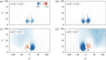
Figure 11. Contours of coherent Reynolds stresses in the cross-stream plane ( $r_{x}=0$ ): (a)  $\langle u_{s}|_{\unicode[STIX]{x1D706}_{x}}^{nl}\rangle \langle v_{s}|_{\unicode[STIX]{x1D706}_{x}}^{nl}\rangle$ ; (b)  $\langle u_{s}|_{\unicode[STIX]{x1D706}_{x}}^{pl}\rangle \langle v_{s}|_{\unicode[STIX]{x1D706}_{x}}^{pl}\rangle$ ; (c)  $\langle u|_{\unicode[STIX]{x1D706}_{x}}^{nl}\rangle \langle v|_{\unicode[STIX]{x1D706}_{x}}^{nl}\rangle$ ; (d)  $\langle u|_{\unicode[STIX]{x1D706}_{x}}^{pl}\rangle \langle v|_{\unicode[STIX]{x1D706}_{x}}^{pl}\rangle$ . Vectors indicate the in-plane velocity components of the corresponding event. The black dot indicates the reference position, $y_{ref}^{+}=14.5$ . The contour levels are $\pm (0.05:0.025:0.4)$ .

For the small-scale wall-normal components (figure 9 a,b), the positive and negative regions (upwash and downwash motions) were intense under the positive- $u_{l}$ event compared to the negative- $u_{l}$ event; the maximum values of $\langle v_{s}|_{\unicode[STIX]{x1D706}_{x}}^{pl}\rangle ^{+}$ and $\langle v_{s}|_{\unicode[STIX]{x1D706}_{x}}^{nl}\rangle ^{+}$ were 0.5 and 0.4, respectively. For the small-scale spanwise components (figure 10 a,b), the negative- and positive- $w_{s}$ region was located above and below the centre of the vortex. In particular, the positive- $w_{s}$ region was noticeably strengthened under the positive- $u_{l}$ event, whereas the negative- $w_{s}$ region had comparable magnitudes under the negative- and positive- $u_{l}$ event (compare figure 10 a with 10 b); the minimum value was $-0.6$ for both events, while the maximum values of $\langle w_{s}|_{\unicode[STIX]{x1D706}_{x}}^{pl}\rangle ^{+}$ and $\langle w_{s}|_{\unicode[STIX]{x1D706}_{x}}^{nl}\rangle ^{+}$ were 0.9 and 0.6, respectively. These observations indicated that the amplitude attenuation and amplification of the small-scale cross-stream components were attributed to the dependence of the streamwise vortical motions on the $u_{l}$ event.

A noteworthy feature of figure 10(a,b) is that only the positive- $w_{s}$ region ( $y<y_{ref}$ ) was strengthened under the positive- $u_{l}$ event. In contrast to the modulation of $v_{s}$ (i.e. amplification of $v_{s}$ on both sides of the swirling motions in figure 9 b), this behaviour indicated that the large-scale high-speed structure influenced the amplitude of $w_{s}$ below the centre of the vortical motions. This phenomenon was further investigated by conditionally averaging the total velocity fluctuations ( $\boldsymbol{u}$ ), which possessed the large-sale components. The educed cross-stream components of the total fluctuations ( $\langle v|_{\unicode[STIX]{x1D706}_{x}}\rangle$ and $\langle w|_{\unicode[STIX]{x1D706}_{x}}\rangle$ ) are presented in figures 9(c,d) and 10(c,d). The cross-stream components clearly differed from the educed small scales (compare figures 9 a,b and 10 a,b respectively with figures 9 c,d and 10 c,d) due to the presence of large scales. Note that the educed total velocity fluctuations for the weak $u_{l}$ (figure 17 b) represent an absence of large-scale circulations, revealing that the large-scale features described here were important for explaining the differences between the flow fields obtained under the negative and positive $u_{l}$ event.

In figure 9(c,d), the wall-normal component included wide regions of positive and negative $v$ beyond the buffer region, indicative of the upwash and downwash motions associated with the outer ejection and sweep events induced by large-scale structures. Likewise, congregative and dispersive motions, which were represented by the intense negative- $w$ regions above $y_{ref}$ , were observed in the spanwise component for the negative- and positive- $u_{l}$ event, respectively (figure 10 c,d). The magnitudes of the positive $w$ ( $y<y_{ref}$ ) in figure 10(c,d) were similar to the positive $w_{s}$ in figure 10(a,b); the maximum values of $\langle w|_{\unicode[STIX]{x1D706}_{x}}^{pl}\rangle ^{+}$ and $\langle w|_{\unicode[STIX]{x1D706}_{x}}^{nl}\rangle ^{+}$ were 0.9 and 0.6, respectively, consistent with those of $\langle w_{s}|_{\unicode[STIX]{x1D706}_{x}}^{pl}\rangle ^{+}$ and $\langle w_{s}|_{\unicode[STIX]{x1D706}_{x}}^{nl}\rangle ^{+}$ . In other words, the large-scale component was not superimposed on the spanwise velocity fluctuations below the centre of the modulated vortical structures, whereas the large-scale spanwise motions appeared above the centre of the modulated vortical structures. Along the spanwise direction, in particular, the negative- $w$ region of $\langle w|_{\unicode[STIX]{x1D706}_{x}}^{pl}\rangle ^{+}$ prevailed with a greater magnitude compared to that of $\langle w|_{\unicode[STIX]{x1D706}_{x}}^{nl}\rangle ^{+}$ . This result was reminiscent of the strong spanwise motions within the footprint of positive $u_{l}$ (cf. figure 7 d). The near-wall spanwise motions induced by positive- $u_{l}$ structures strengthened the opposite spanwise motion (positive- $w_{s}$ region in figure 10 b) below the centre of the streamwise vortical structures, whereas the small-scale spanwise component was relatively weakened under the negative- $u_{l}$ event due to the relatively weak spanwise motions.

Figure 12. Contours of coherent Reynolds stresses in the cross-stream plane ( $r_{x}=0$ ): (a)  $\langle u_{s}|_{\unicode[STIX]{x1D706}_{x}}^{nl}\rangle \langle w_{s}|_{\unicode[STIX]{x1D706}_{x}}^{nl}\rangle$ ; (b)  $\langle u_{s}|_{\unicode[STIX]{x1D706}_{x}}^{pl}\rangle \langle w_{s}|_{\unicode[STIX]{x1D706}_{x}}^{pl}\rangle$ ; (c)  $\langle u|_{\unicode[STIX]{x1D706}_{x}}^{nl}\rangle \langle w|_{\unicode[STIX]{x1D706}_{x}}^{nl}\rangle$ ; (d)  $\langle u|_{\unicode[STIX]{x1D706}_{x}}^{pl}\rangle \langle w|_{\unicode[STIX]{x1D706}_{x}}^{pl}\rangle$ . Vectors indicate the in-plane velocity components of the corresponding event. The black dot indicates the reference position, $y_{ref}^{+}=14.5$ . The contour levels are $\pm (0.05:0.05:0.5)$ .

Figures 11(a,b) and 12(a,b) present a wide view of the Reynolds stresses associated with the small-scale components. Figure 11(a,b) indicated that intense regions of negative $\langle u_{s}|_{\unicode[STIX]{x1D706}_{x}}\rangle \langle v_{s}|_{\unicode[STIX]{x1D706}_{x}}\rangle$ appeared on both sides of the vortical structure. The magnitude of these regions, in particular, was noticeably greater for the positive- $u_{l}$ event; the minimum values of $\langle u_{s}|_{\unicode[STIX]{x1D706}_{x}}^{nl}\rangle \langle v_{s}|_{\unicode[STIX]{x1D706}_{x}}^{nl}\rangle$ and $\langle u_{s}|_{\unicode[STIX]{x1D706}_{x}}^{pl}\rangle \langle v_{s}|_{\unicode[STIX]{x1D706}_{x}}^{pl}\rangle$ were $-0.37$ and $-0.59$ , respectively. These results revealed that the amplification of the small-scale velocity components under the footprints of the positive- $u_{l}$ structures enhanced vertical momentum transport. Furthermore, the magnitudes of $\langle u_{s}|_{\unicode[STIX]{x1D706}_{x}}^{pl}\rangle \langle w_{s}|_{\unicode[STIX]{x1D706}_{x}}^{pl}\rangle$ below the centre of the vortex exceeded those of $\langle u_{s}|_{\unicode[STIX]{x1D706}_{x}}^{nl}\rangle \langle w_{s}|_{\unicode[STIX]{x1D706}_{x}}^{nl}\rangle$ (figure 12 a,b), indicating that the spanwise transport of the streamwise momentum was also dominant for the positive- $u_{l}$ event. The intense regions of $\langle u_{s}|_{\unicode[STIX]{x1D706}_{x}}^{pl}\rangle \langle w_{s}|_{\unicode[STIX]{x1D706}_{x}}^{pl}\rangle$ arose from the amplification of the positive $w_{s}$ as observed in figure 10(b).

Figure 11(c,d) displays the cross-stream plane of $\langle u|_{\unicode[STIX]{x1D706}_{x}}^{nl}\rangle \langle v|_{\unicode[STIX]{x1D706}_{x}}^{nl}\rangle$ and $\langle u|_{\unicode[STIX]{x1D706}_{x}}^{pl}\rangle \langle v|_{\unicode[STIX]{x1D706}_{x}}^{pl}\rangle$ . The outer ejection and sweep motions were observed in contrast to figure 11(a,b). Note that the outer ejection and sweep motions were not observed under the weak- $u_{l}$ condition (see figure 17 b). Figure 12(c,d) shows the large spanwise extent of the positive and negative regions of $\langle u|_{\unicode[STIX]{x1D706}_{x}}\rangle \langle w|_{\unicode[STIX]{x1D706}_{x}}\rangle$ above the reference position. Given the spanwise direction of the inserted vectors (negative $w$ for the negative- and positive- $u_{l}$ conditions), the modulated vortical structures under the influence of negative or positive $u_{l}$ were embedded within the streamwise velocity, which was lower or higher than the mean streamwise velocity. In addition, the large spanwise extent of the positive and negative regions indicated the presence of the congregative and dispersive motions under the footprints of negative and positive $u_{l}$ , respectively. The strong spanwise motions for the positive- $u_{l}$ event produced a larger maximum magnitude of $\langle u|_{\unicode[STIX]{x1D706}_{x}}^{pl}\rangle \langle w|_{\unicode[STIX]{x1D706}_{x}}^{pl}\rangle ^{+}$ ( ${\approx}1.6$ ) compared to that of $\langle u|_{\unicode[STIX]{x1D706}_{x}}^{nl}\rangle \langle w|_{\unicode[STIX]{x1D706}_{x}}^{nl}\rangle ^{+}$ ( ${\approx}1.3$ ). This result demonstrated that the modulated vortical motions lay within the outer large-scale circulations, and that the vertical and lateral momentum transports were enhanced or diminished in connection with the AM of the small-scale velocity fluctuations. Note that the flow fields associated with the modulated $\unicode[STIX]{x1D706}_{y}$ showed similar results to $\unicode[STIX]{x1D706}_{x}$ (not shown here), indicating that the intense spanwise motions under the positive- $u_{l}$ event contributed to the amplification of the velocity fields around the modulated  $\unicode[STIX]{x1D706}_{y}$ .

6 Influence of large-scale motions on the skin-friction coefficient

In this section, we analyse the contribution of the modulated vortical motions to the skin friction. Since the near-wall vortical structures were responsible for the Reynolds shear stress (Robinson Reference Robinson1991) and the Reynolds shear stress was directly related to the skin friction (Fukagata, Iwamoto & Kasagi Reference Fukagata, Iwamoto and Kasagi2002), the amplification and attenuation of the swirling motions, and also their associated velocity fields (§ 5) would have an influence on the local skin-friction coefficient ( $C_{f}$ ). In order to quantify the contribution of the modulated vortical motions on $C_{f}$ , we used a new decomposition method for $C_{f}$ as suggested by Yoon et al. (Reference Yoon, Ahn, Hwang and Sung2016a ). The details of the derivation procedure are described in Yoon et al. (Reference Yoon, Ahn, Hwang and Sung2016a ). Using this method, $C_{f}$ could be decomposed into five parts,

(6.1) $$\begin{eqnarray}\displaystyle C_{f} & = & \displaystyle \underbrace{\int _{0}^{1}2\left(1-\frac{y}{\unicode[STIX]{x1D6FF}}\right)\frac{\langle v\unicode[STIX]{x1D714}_{z}\rangle }{U_{\infty }^{2}/\unicode[STIX]{x1D6FF}}\,\text{d}\left(\frac{y}{\unicode[STIX]{x1D6FF}}\right)}_{C_{f1}}+\underbrace{\int _{0}^{1}2\left(1-\frac{y}{\unicode[STIX]{x1D6FF}}\right)\frac{\langle -w\unicode[STIX]{x1D714}_{y}\rangle }{U_{\infty }^{2}/\unicode[STIX]{x1D6FF}}\,\text{d}\left(\frac{y}{\unicode[STIX]{x1D6FF}}\right)}_{C_{f2}}\nonumber\\ \displaystyle & & \displaystyle +\,\underbrace{\frac{\unicode[STIX]{x1D708}\unicode[STIX]{x1D6FF}}{U_{\infty }^{2}}\left.\frac{\unicode[STIX]{x2202}\unicode[STIX]{x1D6FA}_{z}}{\unicode[STIX]{x2202}y}\right|_{y=0}}_{C_{f3}}+\underbrace{\frac{\unicode[STIX]{x1D708}}{U_{\infty }^{2}}\int _{0}^{1}-2\unicode[STIX]{x1D6FA}_{z}\,\text{d}\left(\frac{y}{\unicode[STIX]{x1D6FF}}\right)}_{C_{f4}}+\underbrace{\int _{0}^{1}\left(1-\frac{y}{\unicode[STIX]{x1D6FF}}\right)^{2}\langle I_{x}\rangle \frac{\unicode[STIX]{x1D6FF}^{2}}{U_{\infty }^{2}}\,\text{d}\left(\frac{y}{\unicode[STIX]{x1D6FF}}\right)}_{C_{f5}},\qquad\end{eqnarray}$$

(6.2) $$\begin{eqnarray}\langle I_{x}\rangle =\frac{\unicode[STIX]{x2202}}{\unicode[STIX]{x2202}x}(U\unicode[STIX]{x1D6FA}_{z}+\langle u\unicode[STIX]{x1D714}_{z}\rangle -\langle w\unicode[STIX]{x1D714}_{x}\rangle )+\frac{\unicode[STIX]{x2202}}{\unicode[STIX]{x2202}y}(V\unicode[STIX]{x1D6FA}_{z})-\unicode[STIX]{x1D708}\frac{\unicode[STIX]{x2202}^{2}\unicode[STIX]{x1D6FA}_{z}}{\unicode[STIX]{x2202}x^{2}}.\qquad\end{eqnarray}$$

The first and second terms ( $C_{f1}$ and $C_{f2}$ ) represent the contributions of the velocity–vorticity correlations $\langle v\unicode[STIX]{x1D714}_{z}\rangle$ and $\langle w\unicode[STIX]{x1D714}_{y}\rangle$ . The third and fourth terms ( $C_{f3}$ and $C_{f4}$ ) indicate the contributions of the molecular diffusion at the wall and the molecular transfer due to the mean vorticity, respectively. The last term ( $C_{f5}$ ) is the contribution of a spatial development term $\langle I_{x}\rangle$ (6.2). In the present study, we focus on the second term ( $C_{f2}$ ) which was the dominant contribution to $C_{f}$ . Furthermore, the velocity–vorticity correlation $\langle -w\unicode[STIX]{x1D714}_{y}\rangle$ was associated with the change-of-scale effect related to the vortex-stretching force. Using a mixing length representation, $\langle -w\unicode[STIX]{x1D714}_{y}\rangle$ is scaled as $u^{\ast }(\unicode[STIX]{x2202}U/\unicode[STIX]{x2202}y)(\unicode[STIX]{x2202}l/\unicode[STIX]{x2202}y)$ , where $u^{\ast }$ is the characteristic velocity and $l$ is the length scale. $\langle -w\unicode[STIX]{x1D714}_{y}\rangle$ can be interpreted as a body force related to the change of scale of eddies ( $\unicode[STIX]{x2202}l/\unicode[STIX]{x2202}y$ ) with the vorticity of $O(\unicode[STIX]{x2202}U/\unicode[STIX]{x2202}y)$ (Tennekes & Lumley Reference Tennekes and Lumley1972). The profile of $\langle -w\unicode[STIX]{x1D714}_{y}\rangle$ had a positive peak in the near-wall region due to either (i)  $w>0$ and $\unicode[STIX]{x1D714}_{y}<0$ or (ii)  $w<0$ and $\unicode[STIX]{x1D714}_{y}>0$ . Physically, a positive value of $\langle -w\unicode[STIX]{x1D714}_{y}\rangle$ was consistent with the two legs of hairpin-like vortices (or streamwise vortices) moving close to one another, and then stretching as they advected from the wall. In addition, $\langle -w\unicode[STIX]{x1D714}_{y}\rangle$ was closely related to the AM (change of length scale) of the small scales by the large-scale motions (Chin et al. Reference Chin, Philip, Klewicki, Ooi and Marusic2014; Hwang, Lee & Sung Reference Hwang, Lee and Sung2016a ). Hence, the contribution of the modulated vortical motions to $C_{f}$ was directly quantified by computing the $C_{f2}$ term.

We first evaluated the velocity–vorticity correlation between the spanwise velocity and wall-normal vorticity fluctuations ( $\langle -w\unicode[STIX]{x1D714}_{y}\rangle$ ) conditioned on the strength of $u_{l}$ similar to (4.2). The correlation can be computed as

(6.3) $$\begin{eqnarray}\langle -w\unicode[STIX]{x1D714}_{y}(u_{l},y)\rangle =\frac{\displaystyle \sum w(y)\unicode[STIX]{x1D714}_{y}(y)|_{u_{l}}}{N[u_{l}(y)]}.\end{eqnarray}$$

Figure 13(a) shows the contour of $\langle -w\unicode[STIX]{x1D714}_{y}(u_{l},y)\rangle ^{+}$ . In the near-wall region, intense regions appeared for the positive $u_{l}$ and $\langle -w\unicode[STIX]{x1D714}_{y}(u_{l},y)\rangle ^{+}$ decreased with decreasing $u_{l}$ . The wall-normal vortical motion within the footprint of $u_{l}$ and its associated spanwise velocity were modulated by $u_{l}$ (§ 5), which, in turn, contributed to the dependence of $\langle -w\unicode[STIX]{x1D714}_{y}\rangle$ on the strength of $u_{l}$ . Unlike with $\unicode[STIX]{x1D706}_{x}$ and $\unicode[STIX]{x1D706}_{y}$ (figure 5), $\langle -w\unicode[STIX]{x1D714}_{y}(u_{l},y)\rangle ^{+}$ decreased rapidly beyond $y^{+}\approx 50$ , regardless of $u_{l}$ . Figure 13(b) shows the profiles of $\langle -w\unicode[STIX]{x1D714}_{y}(u_{l},y)\rangle ^{+}$ for $u_{l}^{+}=-2$ , 0 and 2. The profiles reached a distinct peak at $y^{+}\approx 12$ and decayed close to zero as $y$ increased. The inset in figure 13(b) plots a zoomed-in view of the region above $y^{+}\approx 50$ . The profile of $\langle -w\unicode[STIX]{x1D714}_{y}(u_{l},y)\rangle ^{+}$ for $u_{l}^{+}=-2$ crossed zero at $y^{+}\approx 100$ and attained a constant negative value, indicating that the vortex stretching in this region negatively contributed to $C_{f2}$ . In other words, the value of $C_{f2}$ in this region was negative as a result of integrating $\langle -w\unicode[STIX]{x1D714}_{y}\rangle$ from $y^{+}=100$ to $y^{+}=\unicode[STIX]{x1D6FF}^{+}$ , which was attributed to a reduction in the skin friction. For $u_{l}^{+}=2$ , by contrast, the profile of $\langle -w\unicode[STIX]{x1D714}_{y}\rangle$ was positive and reached a higher magnitude along the wall-normal direction; thus, the vortex stretching (amplified vortical motions) under the influence of positive $u_{l}$ enhanced  $C_{f}$ .

Figure 13. (a) Correlation between the spanwise velocity fluctuations and the wall-normal velocity fluctuations conditioned on the large-scale fluctuations along the wall-normal direction, $\langle -w\unicode[STIX]{x1D714}_{y}(u_{l},y)\rangle ^{+}$ . (b) Profiles of $\langle -w\unicode[STIX]{x1D714}_{y}(u_{l},y)\rangle ^{+}$ along the wall-normal direction for $u_{l}^{+}=-2$ , 0 and 2. (c) Dependence of the skin friction induced by $\langle -w\unicode[STIX]{x1D714}_{y}(u_{l},y)\rangle$ on the large-scale fluctuations, $\langle C_{f2}(u_{l})\rangle$ . The dashed lines indicate $C_{f2}$ in (6.1). (d) Contribution of $\langle C_{f2}(u_{l})\rangle$ to $C_{f2}$ , $C_{f2}^{con}(u_{l})$ .

Next, the frictional drag induced by the modulated $\langle -w\unicode[STIX]{x1D714}_{y}\rangle$ was examined by obtaining the second term in (6.1) as a function of  $u_{l}$ ,

(6.4) $$\begin{eqnarray}\langle C_{f2}(u_{l})\rangle =\int _{0}^{1}2\left(1-\frac{y}{\unicode[STIX]{x1D6FF}}\right)\frac{\langle -w\unicode[STIX]{x1D714}_{y}(u_{l},y)\rangle }{U_{\infty }^{2}/\unicode[STIX]{x1D6FF}}\,\text{d}\left(\frac{y}{\unicode[STIX]{x1D6FF}}\right).\end{eqnarray}$$

In figure 13(c), the skin friction induced by the vortex stretching effect (or change-of-scale effect) varied with the strength of $u_{l}$ , indicating that the modulation of vortical motions was directly attributed to the dependence of the local skin friction on the large-scale structures. Here, the horizontal line indicates $C_{f2}$ in (6.1). The value of $\langle C_{f2}(u_{l})\rangle$ for the positive $u_{l}$ exceeded the value of $C_{f2}$ , whereas this trend was reversed for the negative $u_{l}$ . The amplified vortical motions within the footprint of positive $u_{l}$ induced the high skin friction, more than 3 times greater than the mean $C_{f2}$ . Conversely, the vortical motions, which were attenuated within the footprint of the negative $u_{l}$ , contributed to the low skin friction. This observation was connected to the relationship between the footprints of the large-scale low-speed structure and the large-scale low skin-friction event (Hutchins et al. Reference Hutchins, Monty, Ganapathisubramani, Ng and Marusic2011), as well as with the locally low or high $Re_{\unicode[STIX]{x1D70F}}$ within the negative- or positive- $u_{l}$ footprints (Chernyshenko et al. Reference Chernyshenko, Marusic and Mathis2012; Ganapathisubramani et al. Reference Ganapathisubramani, Hutchins, Monty, Chung and Marusic2012).

Given that the p.d.f. of $u_{l}$ was antisymmetric with respect to $u_{l}^{+}=0$ (figure 4), we considered the contribution of $\langle C_{f2}(u_{l})\rangle$ to $C_{f2}$ . The contribution of $\langle C_{f2}(u_{l})\rangle$ ( $C_{f2}^{con}$ ) could be computed according to

(6.5) $$\begin{eqnarray}\displaystyle & \displaystyle C_{f2}^{con}(u_{l})=\frac{1}{C_{f2}}\int _{0}^{1}2\left(1-\frac{y}{\unicode[STIX]{x1D6FF}}\right)\frac{\langle -w\unicode[STIX]{x1D714}_{y}(u_{l},y)\rangle }{U_{\infty }^{2}/\unicode[STIX]{x1D6FF}}C(u_{l},y)\,\text{d}\left(\frac{y}{\unicode[STIX]{x1D6FF}}\right), & \displaystyle\end{eqnarray}$$

(6.6) $$\begin{eqnarray}\displaystyle & \displaystyle C(u_{l},y)=\frac{N[u_{l}(y)]}{\displaystyle \sum N[u_{l}(y)]}, & \displaystyle\end{eqnarray}$$

(6.7) $$\begin{eqnarray}\displaystyle & \displaystyle \mathop{\sum }_{u_{l}=-\infty }^{\infty }C_{f2}^{con}(u_{l})=\frac{C_{f2}}{C_{f2}}=1. & \displaystyle\end{eqnarray}$$

As shown in figure 13(d), the plot of $C_{f2}^{con}(u_{l})$ was not symmetric with respect to $u_{l}^{+}=0$ . A peak appeared at $u_{l}^{+}=0$ due to the dominance of the weak- $u_{l}$ event (i.e. a peak in the p.d.f. of $u_{l}$ was located in the vicinity of $u_{l}^{+}\approx 0$ in figure 4). The contribution of $u_{l}<0$ was quite small compared to that of $u_{l}>0$ . A negative contribution was observed in the range $u_{l}^{+}<-2.3$ because $\langle -w\unicode[STIX]{x1D714}_{y}\rangle <0$ in the outer region became dominant compared to $\langle -w\unicode[STIX]{x1D714}_{y}\rangle >0$ in the near-wall region. As a result, the cumulative contribution of $u_{l}^{+}<-2$ was nearly zero, whereas the vortex stretching within $u_{l}^{+}>2$ was responsible for 15 % of the contribution to $C_{f2}$ ; the cumulative contribution of $u_{l}^{+}<-1$ and $u_{l}^{+}>1$ was 11 % and 36 %, respectively. The intense spanwise motion of the positive $u_{l}$ in the near-wall region enhanced the small-scale velocity fluctuations as well as the vortical motions, which were related to the intense vortex-stretching effect. As a result, the amplification effect by the positive- $u_{l}$ structure considerably contributed to the skin friction, in contrast to the negative- $u_{l}$ structures, and thus manipulating the near-wall spanwise motions induced by outer large-scale structures could offer a new strategy for controlling turbulence.

6.1 Analysis of a drag-reduced turbulent flow

The AM effect of the large-scale structures on the vortical motions was quantified by integrating the wall-normal distribution of $\langle -w\unicode[STIX]{x1D714}_{y}\rangle$ according to the strength of $u_{l}$ in (6.5). The contribution of the AM to $C_{f}$ was varied according to the strength of $u_{l}$ . In particular, the frictional drag induced by the positive- $u_{l}$ event was significantly larger than that by the negative- $u_{l}$ event. To explore further, a drag-reduced turbulent flow was examined. We used two DNS datasets for the turbulent channel with no-slip and slip condition at a given bulk Reynolds number $Re_{b}=U_{bulk}\unicode[STIX]{x1D6FF}/\unicode[STIX]{x1D708}=10\,333$ (Yoon et al. Reference Yoon, Hwang, Lee, Sung and Kim2016b ). Although the drag reduction was achieved due to the slip boundary condition, we can examine the variation of the skin friction induced by the modulated vortical motions in the drag-reduced flow – especially the high skin friction under the large-scale high-speed structures observed in figure 13. This approach could provide an evidence of controlling the AM effect on $C_{f}$ by manipulating the high-speed structures. Figure 14(a,c) shows the contours of $\langle -w\unicode[STIX]{x1D714}_{y}(u_{l},y)\rangle$ for the no-slip and slip wall. Here, the quantities were normalized by the bulk mean velocity $U_{bulk}$ and the channel half-height $\unicode[STIX]{x1D6FF}$ . At the no-slip wall, $u_{l}/U_{bulk}=0.17$ was consistent with $u_{l}^{+}=3$ . Irrespective of $u_{l}$ , the magnitude of $\langle -w\unicode[STIX]{x1D714}_{y}(u_{l},y)\rangle$ in figure 14(c) was lower than that in figure 14(a). The vortex-stretching force decreased in the channel flow with the slip condition. Note that the overall drag under the slip condition was reduced by 35 % relative to the flow with the no-slip condition (Yoon et al. Reference Yoon, Hwang, Lee, Sung and Kim2016b ). In other words, the reduced magnitude of the vortex-stretching force, which was affected by the large-scale low- and high-speed events, contributed to the overall drag reduction in the slip wall.

Figure 14. (a,c) Correlation between the spanwise velocity fluctuations and the wall-normal velocity fluctuations conditioned on the large-scale fluctuations along the wall-normal direction, $\langle -w\unicode[STIX]{x1D714}_{y}(u_{l},y)\rangle \unicode[STIX]{x1D6FF}/U_{bulk}^{2}$ : (a) no-slip wall; (c) slip wall. (b) Dependence of the skin friction induced by $\langle -w\unicode[STIX]{x1D714}_{y}(u_{l},y)\rangle$ on the large-scale fluctuations, $\langle C_{f2}(u_{l})\rangle$ . The dashed lines represent $C_{f2}$ in (6.1). (d) Contribution of the change in $\langle C_{f2}(u_{l})\rangle$ to the reduced $C_{f2}$ , $\unicode[STIX]{x0394}C_{f2}$ (black) and cumulative distribution of $\unicode[STIX]{x0394}C_{f2}(u_{l})$ , $\unicode[STIX]{x0394}C_{f2}^{cum}$ (blue).

The influence of the large-scale motions on the skin friction under the no-slip and slip wall was compared by plotting $\langle C_{f2}(u_{l})\rangle$ (6.4) for each case in figure 14(b). The horizontal dashed lines in figure 14(b) represent the contribution of $\langle -w\unicode[STIX]{x1D714}_{y}\rangle$ to the total $C_{f}$ ; the second term on the right-hand side of (6.1) for the no-slip ( $C_{f2,n}$ ) and slip wall ( $C_{f2,s}$ ). Although the plot of $\langle C_{f2}(u_{l})\rangle$ for the slip wall fell below that for the no-slip wall, the difference in $\langle C_{f2}(u_{l})\rangle$ between the no-slip and slip wall varied with the strength of $u_{l}$ . For the intense negative $u_{l}$ ( $u_{l}/U_{bulk}\approx -0.17$ ), there was a slight difference in $\langle C_{f2}(u_{l})\rangle$ between the no-slip and slip wall. However, the difference started to become noticeable as $u_{l}$ increased. Above $u_{l}/U_{bulk}>0.1$ , in particular, the difference in $\langle C_{f2}(u_{l})\rangle$ exceeded the reduced $C_{f2}$ ( $=C_{f2,n}-C_{f2,s}\approx 4.1\times 10^{-3}$ ). The skin friction induced by the vortex-stretching effect decreased at the slip wall, but the amount of change in the skin friction was significant for the positive $u_{l}$ . To further explore this observation, the contribution of the change in $\langle C_{f2}(u_{l})\rangle$ to the reduced $C_{f2}$ was defined as,

(6.8) $$\begin{eqnarray}\unicode[STIX]{x0394}C_{f2}(u_{l})=\frac{C_{f2,n}C_{f2,n}^{con}(u_{l})-C_{f2,s}C_{f2,s}^{con}(u_{l})}{C_{f2,n}-C_{f2,s}},\end{eqnarray}$$

where $C_{f2,n}^{con}$ and $C_{f2,s}^{con}$ are the contributions of $\langle C_{f2}(u_{l})\rangle$ to $C_{f2}$ (6.5) for the no-slip and slip walls, respectively. $\unicode[STIX]{x0394}C_{f2}(u_{l})$ indicates the difference in the frictional drag induced by $u_{l}$ between the no-slip and slip walls and its contribution to the reduced $C_{f}$ . The black line in figure 14(d) represents $\unicode[STIX]{x0394}C_{f2}(u_{l})$ . Although the contribution to the reduced $C_{f2}$ was largest in the vicinity of $u_{l}\approx 0$ , $\unicode[STIX]{x0394}C_{f2}(u_{l})$ was not symmetric with respect to $u_{l}\approx 0$ . As the magnitude of $u_{l}$ increased, $\unicode[STIX]{x0394}C_{f2}(u_{l})$ for $u_{l}<0$ declined to a greater extent than $\unicode[STIX]{x0394}C_{f2}(u_{l})$ for $u_{l}>0$ . This behaviour was evident in the cumulative distribution of $\unicode[STIX]{x0394}C_{f2}(u_{l})$ in figure 14(d). For the intense positive $u_{l}$ region, $u_{l}/U_{bulk}>0.1$ ( $u_{l}^{+}>2$ ), the reduction in the skin friction induced by the amplified vortical motions was responsible for 22 % of the reduced $C_{f2}$ ; cf. for $u_{l}/U_{bulk}>0.05$ , $\unicode[STIX]{x0394}C_{f2}^{cum}=0.6$ . This result indicated that the amplification of the vortical motions within the footprint of positive $u_{l}$ was markedly diminished compared to the attenuation effect produced by the negative $u_{l}$ , which ultimately contributed to the total drag reduction at the slip wall. In this manner, manipulating the positive- $u_{l}$ structure, which amplified the near-wall motions through the associated intense spanwise motions (§ 5) might provide a means for controlling turbulence. The analysis described in this section serves as a reliable measure for evaluating new control strategies by manipulating the AM effects of large-scale motions.