


1. Introduction
Flow near rigid boundaries is often affected by surface roughness and this has stimulated numerous studies aimed at quantifying the effect of roughness geometry on flow. However, these studies are still inconclusive as the multiple scales involved make it difficult to identify the most important geometric roughness parameters. The influence of rough surfaces on the friction exerted by fluids is of interest in a wide variety of fields, including turbomachinery, river flows, meteorological applications and many others. The reader is referred to Jiménez (Reference Jiménez2004) and Chung et al. (Reference Chung, Hutchings, Schultz and Flack2021) for thorough reviews of the subject. The first systematic experimental study in this field was carried out by Nikuradse (Reference Nikuradse1933), who, in order to use an easily measurable roughness, glued sand of constant diameter to the inside wall of smooth pipes, so that a single length (the grain diameter) was suitable for describing the roughness size. Sand roughness size is now widely used as a measure of surface roughness. For ordinary pipes, roughness has a complex shape that cannot be described by a single length. Nevertheless, for these cases an equivalent sand roughness height (
 $k_s$
) is used, which is defined as the diameter of the Nikuradse pipe sand grain that produces the same friction factor as the pipe under consideration in the fully rough turbulent regime. A weakness of this approach is that there is no guarantee that the matching of friction factors in the fully rough regime also provides a good match in the transitional rough regime.
$k_s$
) is used, which is defined as the diameter of the Nikuradse pipe sand grain that produces the same friction factor as the pipe under consideration in the fully rough turbulent regime. A weakness of this approach is that there is no guarantee that the matching of friction factors in the fully rough regime also provides a good match in the transitional rough regime.
The approach of Nikuradse (Reference Nikuradse1933) to describe surface roughness belongs to the discrete approach (Stewart et al. Reference Stewart, Stuart, Nikora, Zampiron and Marusic2019), where surface roughness is described by a set of linear scales, and although it has proven useful in several engineering applications, it is not entirely satisfactory for a detailed description of the complexity of a rough surface, as a large number of parameters should be considered, such as particle shape, orientation and degree of exposure. However, this is the approach generally used to describe river bed roughness. For example, van Rijn (Reference van Rijn1982) reported that the equivalent sand grain roughness
 $k_s$
is related to
$k_s$
is related to
 $D_{90}$
(
$D_{90}$
(
 $90\, \%$
of the sample volume is made up of all particles with a diameter smaller than
$90\, \%$
of the sample volume is made up of all particles with a diameter smaller than
 $D_{90}$
), whereas Whiting & Dietrich (Reference Whiting and Dietrich1990) assumed that
$D_{90}$
), whereas Whiting & Dietrich (Reference Whiting and Dietrich1990) assumed that
 $k_s$
is proportional to
$k_s$
is proportional to
 $D_{84}$
.
$D_{84}$
.
Another way of describing surface roughness is based on the continuous approach, where the roughness is considered as a random field of surface elevations (Nikora, Goring & Biggs Reference Nikora, Goring and Biggs1998; Stewart et al. Reference Stewart, Stuart, Nikora, Zampiron and Marusic2019) described by the moments of the frequency distribution and by the power spectral density (PSD). The choice between discrete and continuous approaches mainly concerns rough surfaces formed by granular elements, as in the case of river beds, whereas in industrial applications the continuous approach is usually the only way to describe a rough surface. In line with the continuous approach, Flack & Schultz (Reference Flack and Schultz2010) analysed data from several surface roughnesses and reported that the equivalent sand roughness is given by
 $k_s=4.43 k_{rms}(1+sk)^{1.37}$
, where
$k_s=4.43 k_{rms}(1+sk)^{1.37}$
, where
 $k_{rms}$
and
$k_{rms}$
and
 $sk$
are the root mean square and the skewness of the surface heights, respectively. Nikora et al. (Reference Nikora, Goring and Biggs1998) reported that the heights of the surface roughness of a gravel bed are nearly Gaussian with an isotropic second-order structure function
$sk$
are the root mean square and the skewness of the surface heights, respectively. Nikora et al. (Reference Nikora, Goring and Biggs1998) reported that the heights of the surface roughness of a gravel bed are nearly Gaussian with an isotropic second-order structure function
 $D(\ell )$
proportional to
$D(\ell )$
proportional to
 $\ell ^{2H}$
for sufficiently small spatial separation
$\ell ^{2H}$
for sufficiently small spatial separation
 $\ell$
, where
$\ell$
, where
 $H$
is the Hurst exponent, which those authors determined to be 0.79 for a water-worked gravel bed. This behaviour indicates that, at sufficiently small spatial scales, the surface roughness has the properties of a self-affine fractal surface (Turcotte Reference Turcotte1997; Meakin Reference Meakin1998). Other examples of surface roughness showing self-affinity are the surface of the planet Mars (Orosei et al. Reference Orosei, Bianchi, Coradini, Espinasse, Federico, Ferricioni and Gavrishin2003) and fracture surfaces (Ponson et al. Reference Ponson, Bonamy, Auradou, Mourot, Morel, Bouchaud, Guillot and Hulin2006).
$H$
is the Hurst exponent, which those authors determined to be 0.79 for a water-worked gravel bed. This behaviour indicates that, at sufficiently small spatial scales, the surface roughness has the properties of a self-affine fractal surface (Turcotte Reference Turcotte1997; Meakin Reference Meakin1998). Other examples of surface roughness showing self-affinity are the surface of the planet Mars (Orosei et al. Reference Orosei, Bianchi, Coradini, Espinasse, Federico, Ferricioni and Gavrishin2003) and fracture surfaces (Ponson et al. Reference Ponson, Bonamy, Auradou, Mourot, Morel, Bouchaud, Guillot and Hulin2006).
The effect of roughness on the flow can be assessed by the downward shift
 $\Delta U^{+}$
it produces in the logarithmic velocity profile with respect to the logarithmic law of turbulent flow on a smooth wall, known as the roughness function, which is related to the friction factor. Hereinafter, the superscript
$\Delta U^{+}$
it produces in the logarithmic velocity profile with respect to the logarithmic law of turbulent flow on a smooth wall, known as the roughness function, which is related to the friction factor. Hereinafter, the superscript
 $+$
denotes a quantity which is made dimensionless by the friction velocity
$+$
denotes a quantity which is made dimensionless by the friction velocity
 $u_{\tau }$
or by the viscous length
$u_{\tau }$
or by the viscous length
 $\nu /u_{\tau }$
, where
$\nu /u_{\tau }$
, where
 $\nu$
is the kinematic viscosity. Over the past few decades, several studies have investigated the effect of roughness on
$\nu$
is the kinematic viscosity. Over the past few decades, several studies have investigated the effect of roughness on
 $\Delta U^{+}$
. Napoli, Armenio & De Marchis (Reference Napoli, Armenio and De Marchis2008) considered irregular two-dimensional roughness and showed that
$\Delta U^{+}$
. Napoli, Armenio & De Marchis (Reference Napoli, Armenio and De Marchis2008) considered irregular two-dimensional roughness and showed that
 $\Delta U^{+}$
scales with the effective slope
$\Delta U^{+}$
scales with the effective slope
 $ES$
given by the spatial average of the absolute value of the streamwise surface slope. It can be shown that
$ES$
given by the spatial average of the absolute value of the streamwise surface slope. It can be shown that
 $ES$
is twice the solidity
$ES$
is twice the solidity
 $\varLambda$
(Schlichting Reference Schlichting1936) defined as the ratio between the sum of the area of all roughness elements projected in the plane perpendicular to the flow direction and the horizontal area. Leonardi et al. (Reference Leonardi, Orlandi, Smalley, Djenidi, Paden and Antonia2003) used direct numerical simulation (DNS) to study turbulent flow on two-dimensional square bars placed orthogonally to the flow and found results from which it can be deduced that the maximum of
$\varLambda$
(Schlichting Reference Schlichting1936) defined as the ratio between the sum of the area of all roughness elements projected in the plane perpendicular to the flow direction and the horizontal area. Leonardi et al. (Reference Leonardi, Orlandi, Smalley, Djenidi, Paden and Antonia2003) used direct numerical simulation (DNS) to study turbulent flow on two-dimensional square bars placed orthogonally to the flow and found results from which it can be deduced that the maximum of
 $\Delta U^{+}$
is obtained for
$\Delta U^{+}$
is obtained for
 $\varLambda =0.125$
. According to MacDonald et al. (Reference MacDonald, Chan, Chung, Hutchings and Ooi2016), the value
$\varLambda =0.125$
. According to MacDonald et al. (Reference MacDonald, Chan, Chung, Hutchings and Ooi2016), the value
 $\varLambda =0.15$
separates the sparse regime, where
$\varLambda =0.15$
separates the sparse regime, where
 $\Delta U^{+}$
increases with
$\Delta U^{+}$
increases with
 $\varLambda$
, from the dense regime, where
$\varLambda$
, from the dense regime, where
 $\Delta U^{+}$
decreases with
$\Delta U^{+}$
decreases with
 $\varLambda$
. This value of
$\varLambda$
. This value of
 $\varLambda$
is not very different from 0.125, which maximises
$\varLambda$
is not very different from 0.125, which maximises
 $\Delta U^{+}$
according to the results of Leonardi et al. (Reference Leonardi, Orlandi, Smalley, Djenidi, Paden and Antonia2003). In a numerical study of flow in pipes characterised by a three-dimensional sinusoidal corrugation, Chan et al. (Reference Chan, MacDonald, Chung, Hutchins and Ooi2015) found that
$\Delta U^{+}$
according to the results of Leonardi et al. (Reference Leonardi, Orlandi, Smalley, Djenidi, Paden and Antonia2003). In a numerical study of flow in pipes characterised by a three-dimensional sinusoidal corrugation, Chan et al. (Reference Chan, MacDonald, Chung, Hutchins and Ooi2015) found that
 $\Delta U^+$
depends on a combination of both the roughness height and the effective slope.
$\Delta U^+$
depends on a combination of both the roughness height and the effective slope.
Forooghi et al. (Reference Forooghi, Stroh, Magagnato, Jakirlic and Frohnapfel2017) numerically studied the flow over a rough surface created by distributing roughness elements over a flat surface and found that the flow resistance depends on several parameters, including the skewness and the distribution of the roughness elements, with the staggered distribution giving results closer to a random distribution. The importance of the skewness of the roughness height has also been pointed out by Busse, Thakkar & Sandham (Reference Busse, Thakkar and Sandham2017) who studied the hydrodynamic properties of a graphite surface and a grit-blasted surface and found that positive skewness provides the greatest resistance to flow. Barros, Schultz & Flack (Reference Barros, Schultz and Flack2018) tested surfaces characterised by power spectral slope proportional to
 $k^p$
finding that the surface with the lowest slope (
$k^p$
finding that the surface with the lowest slope (
 $p$
= −0.5) has the largest drag, although this case has the smallest
$p$
= −0.5) has the largest drag, although this case has the smallest
 $k_{rms}$
. This was attributed to the presence of low-wavelength features contributing to
$k_{rms}$
. This was attributed to the presence of low-wavelength features contributing to
 $k_{rms}$
but not to the drag. Forooghi et al. (Reference Forooghi, Frohnapfel, Magagnato and Busse2018) improved the parametric forcing model of Busse & Sandham (Reference Busse and Sandham2012) to be able to reproduce the effect of several rough surface characteristics, including skewness. Stewart et al. (Reference Stewart, Stuart, Nikora, Zampiron and Marusic2019) studied experimentally the hydrodynamic properties of a self-affine surface roughness characterised by three different PSDs with scaling exponents −1, −5/3 and −3. They reported that the friction factor increases as the scaling exponent increases. Guo-Zhen et al. (Reference Guo-Zhen, Chun-Xiao, Hyung and Wei-Xi2020) studied the flow on a regular three-dimensional sinusoidal wall and showed that
$k_{rms}$
but not to the drag. Forooghi et al. (Reference Forooghi, Frohnapfel, Magagnato and Busse2018) improved the parametric forcing model of Busse & Sandham (Reference Busse and Sandham2012) to be able to reproduce the effect of several rough surface characteristics, including skewness. Stewart et al. (Reference Stewart, Stuart, Nikora, Zampiron and Marusic2019) studied experimentally the hydrodynamic properties of a self-affine surface roughness characterised by three different PSDs with scaling exponents −1, −5/3 and −3. They reported that the friction factor increases as the scaling exponent increases. Guo-Zhen et al. (Reference Guo-Zhen, Chun-Xiao, Hyung and Wei-Xi2020) studied the flow on a regular three-dimensional sinusoidal wall and showed that
 $\Delta U^{+}$
scales with the product between the amplitude of the roughness and
$\Delta U^{+}$
scales with the product between the amplitude of the roughness and
 $ES$
. The case of irregular three-dimensional roughness was also considered by Ma, Alamé & Mahesh (Reference Ma, Alamé and Mahesh2021), who carried out DNS on the surface corresponding to the experiments of Flack, Schultz & Barros (Reference Flack, Schultz and Barros2020).
$ES$
. The case of irregular three-dimensional roughness was also considered by Ma, Alamé & Mahesh (Reference Ma, Alamé and Mahesh2021), who carried out DNS on the surface corresponding to the experiments of Flack, Schultz & Barros (Reference Flack, Schultz and Barros2020).
The importance of roughness distribution, in addition to roughness height, as a factor affecting the roughness function has been highlighted by Thakkar, Busse & Sandham (Reference Thakkar, Busse and Sandham2017) in their DNS studies of flow on surface roughness. A method for determining which roughness parameter has the greater influence on the roughness function was also presented. Excellent agreement with the results of Nikuradse (Reference Nikuradse1933) was obtained by Thakkar, Busse & Sandham (Reference Thakkar, Busse and Sandham2018) in a study of turbulent flow over an industrial grit-blasted surface. Busse & Jelly (Reference Busse and Jelly2020) studied the effect of surface anisotropy, defined as the ratio between the streamwise and spanwise correlation lengths, and found that as this ratio decreases,
 $\Delta U^{+}$
increases. De Marchis et al. (Reference De Marchis, Saccone, Milici and Napoli2020) considered three-dimensional rough surfaces created by superimposing random amplitude sinusoids and determined the flow characteristics using large-eddy simulation. The study showed that no single parameter of the roughness geometry is sufficient to describe the roughness function, but the results showed that
$\Delta U^{+}$
increases. De Marchis et al. (Reference De Marchis, Saccone, Milici and Napoli2020) considered three-dimensional rough surfaces created by superimposing random amplitude sinusoids and determined the flow characteristics using large-eddy simulation. The study showed that no single parameter of the roughness geometry is sufficient to describe the roughness function, but the results showed that
 $\Delta U^{+}$
can be adequately described by a suitable combination of
$\Delta U^{+}$
can be adequately described by a suitable combination of
 $ES$
and
$ES$
and
 $k_{rms}^{+}$
. Portela, Busse & Sandham (Reference Portela, Busse and Sandham2021) used Fourier filtering to create different rough surfaces from a baseline surface. They found that existing correlations mostly predict the roughness function, but also emphasised that these correlations should include information about the spectral distribution to improve accuracy. Recently, the influence of the effective spanwise slope on
$k_{rms}^{+}$
. Portela, Busse & Sandham (Reference Portela, Busse and Sandham2021) used Fourier filtering to create different rough surfaces from a baseline surface. They found that existing correlations mostly predict the roughness function, but also emphasised that these correlations should include information about the spectral distribution to improve accuracy. Recently, the influence of the effective spanwise slope on
 $\Delta U^{+}$
was analysed by Jelly et al. (Reference Jelly, Ramani, Nugroho, Hutchins and Busse2022), who reported that
$\Delta U^{+}$
was analysed by Jelly et al. (Reference Jelly, Ramani, Nugroho, Hutchins and Busse2022), who reported that
 $\Delta U^{+}$
decreases with the effective spanwise slope when all other geometric parameters are held constant. This is probably related to the increasing two-dimensionality of the roughness as the spanwise slope decreases, which creates more obstacles to the flow.
$\Delta U^{+}$
decreases with the effective spanwise slope when all other geometric parameters are held constant. This is probably related to the increasing two-dimensionality of the roughness as the spanwise slope decreases, which creates more obstacles to the flow.
Yang et al. (Reference Yang, Stroh, Chung and Forooghi2022) studied the flow in a minimal channel and reported that, for an irregular roughness, sufficiently accurate predictions can be obtained if the channel size is large enough to contain more than 90 % of the original roughness height spectral energy. Recently, methods based on artificial neural networks are increasingly being used to predict relevant hydrodynamic features of surface roughness, as in Yang et al. (Reference Yang, Stroh, Lee, Bagheri, Frohnapfel and Forooghi2023a
), who constructed a model to predict equivalent sand roughness based on the probability density function and power spectrum of the rough surface. Yang et al. (Reference Yang, Zhang, Yuan and Kunz2023b
) analysed different rough-wall models and concluded that empirical correlations are effective when calibrated and applied to the same type of roughness. Machine learning and physics-based models were also analysed: the former improve as the amount of data increases; the latter are more adaptable, but require all physical aspects to be identified. In a recent study, Busse & Jelly (Reference Busse and Jelly2023) analysed rough surfaces with very high skewness and observed a saturation of roughness effects at the limits of very high skewness. Ramani et al. (Reference Ramani, Schilt, Nugroho, Busse and Jelly2024) critically examined the dependence of the friction factor on the effective slope and showed from experimental measurements that scale roughness less than three times the viscous length has a weak effect on drag, despite its large contribution to
 $ES$
. The larger contribution to drag comes from the slope due to large scale features.
$ES$
. The larger contribution to drag comes from the slope due to large scale features.
Previous studies have shed much light on flows on rough surfaces, but the results are still inconclusive, so there is still room for further knowledge in this area. In this context, the present work aims to better understand how three-dimensional irregular roughness affects the roughness function. The analysis is carried out by DNS and focuses on the effect of the PSD and the root mean square of the surface roughness heights on the flow. In § 2 the geometry of the surface roughness is defined and the numerical approach is described. In § 3 the results of the study are illustrated and in § 4 some conclusions are drawn.
2. The rough surface and the numerical approach
The turbulent flow in a channel with a rough bottom wall is analysed in this study. All lengths that appear from here on have been made dimensionless using the depth
 $h$
of the channel, except where a plus symbol appears in superscript for variables expressed in wall units. A Cartesian coordinate system
$h$
of the channel, except where a plus symbol appears in superscript for variables expressed in wall units. A Cartesian coordinate system
 $(x,y,z)$
is introduced as a reference, with the x–z plane located at the mid-level of the rough bottom wall and the
$(x,y,z)$
is introduced as a reference, with the x–z plane located at the mid-level of the rough bottom wall and the
 $x$
axis pointing in the direction of the flow. The sizes of the fluid domain are denoted as
$x$
axis pointing in the direction of the flow. The sizes of the fluid domain are denoted as
 $L_{x}$
,
$L_{x}$
,
 $L_{y}=1$
and
$L_{y}=1$
and
 $L_{z}$
in the
$L_{z}$
in the
 $x$
,
$x$
,
 $y$
and
$y$
and
 $z$
directions, respectively. The bottom wall is characterised by periodic displacements with respect to
$z$
directions, respectively. The bottom wall is characterised by periodic displacements with respect to
 $y=0$
with periods equal to
$y=0$
with periods equal to
 $L_x$
and
$L_x$
and
 $L_z$
along the
$L_z$
along the
 $x$
and
$x$
and
 $z$
directions, respectively. Therefore, the surface heights
$z$
directions, respectively. Therefore, the surface heights
 $\eta$
can be expressed in Fourier series:
$\eta$
can be expressed in Fourier series:
 \begin{eqnarray} \eta (x,z)=\sum _{m=-M}^{M} \sum _{n=-N}^{N} f(m,n) \exp[{\rm i}(m \kappa _x x+n \kappa _z z)], \end{eqnarray}
where
 $m$
and
$m$
and
 $n$
are integers,
$n$
are integers,
 ${\rm i}$
is the imaginary unit,
${\rm i}$
is the imaginary unit,
 $f(m,n)$
is a complex number,
$f(m,n)$
is a complex number,
 $\kappa _x=2 \pi /L_x$
and
$\kappa _x=2 \pi /L_x$
and
 $\kappa _z=2\pi /L_z$
. Assuming that the spatial average of
$\kappa _z=2\pi /L_z$
. Assuming that the spatial average of
 $\eta$
in the
$\eta$
in the
 $x$
and
$x$
and
 $z$
directions is zero, it follows that
$z$
directions is zero, it follows that
 $f(0,n)=f(m,0)=0$
regardless of the values of
$f(0,n)=f(m,0)=0$
regardless of the values of
 $m$
and
$m$
and
 $n$
. The spatial autocorrelation function of the surface roughness
$n$
. The spatial autocorrelation function of the surface roughness
 $R(\ell _x,\ell _z)$
, where
$R(\ell _x,\ell _z)$
, where
 $\ell _x$
and
$\ell _x$
and
 $\ell _z$
are the spatial separations along the
$\ell _z$
are the spatial separations along the
 $x$
and
$x$
and
 $z$
directions, respectively, is given by
$z$
directions, respectively, is given by
 \begin{eqnarray} R(\ell _x,\ell _z)=\frac {1}{L_xL_z}\int _{0}^{L_x}\int _{0}^{L_z} y(x,z) y(x+\ell _x,z+\ell _z)\, {\rm d}x \,{\rm d}z \nonumber \\ =\sum _{m=-M}^{M}\sum _{n=-N}^{N}|f(m,n)|^2 \exp[{\rm i}(m k_x \ell _x+n k_z \ell _z)]. \end{eqnarray}
Using equation (2.2), the root mean square of the surface height
 $\eta$
is given by
$\eta$
is given by
 $k_{rms}=\sqrt {R(0,0)}$
. The PSD, given by the Fourier transform of the spatial autocorrelation function, can be written as follows:
$k_{rms}=\sqrt {R(0,0)}$
. The PSD, given by the Fourier transform of the spatial autocorrelation function, can be written as follows:
 \begin{eqnarray} \mathrm {PSD}(m \kappa _x, n \kappa _z)=\frac {1}{4 \pi ^2} L_x L_z |f(m,n)|^2. \end{eqnarray}
It is assumed that the PSD depends on the magnitude of the wavenumber
 $|{\boldsymbol {\kappa }}|=\sqrt {(m^2 \kappa _{x}^{2}+n^2 \kappa _{y}^{2})}$
. This choice is made because several natural and artificial roughnesses have a PSD that follows the power law
$|{\boldsymbol {\kappa }}|=\sqrt {(m^2 \kappa _{x}^{2}+n^2 \kappa _{y}^{2})}$
. This choice is made because several natural and artificial roughnesses have a PSD that follows the power law
 $|{\boldsymbol {\kappa }}|^{(-2H-d)}$
over a range of wavenumbers, typical of a self-affine surface characterised by the Hurst exponent
$|{\boldsymbol {\kappa }}|^{(-2H-d)}$
over a range of wavenumbers, typical of a self-affine surface characterised by the Hurst exponent
 $H$
(
$H$
(
 $0\lt H \le 1$
), where
$0\lt H \le 1$
), where
 $d$
is the Euclidean dimension, which in this case is equal to 2 (Meakin Reference Meakin1998). Note that since the PSD depends only on the magnitude of the wavenumber, all surface roughness quantities, including the effective slope, are independent of spatial direction. Five different PSDs were used to generate the surface roughness, the shape of which is shown in figure 1 for
$d$
is the Euclidean dimension, which in this case is equal to 2 (Meakin Reference Meakin1998). Note that since the PSD depends only on the magnitude of the wavenumber, all surface roughness quantities, including the effective slope, are independent of spatial direction. Five different PSDs were used to generate the surface roughness, the shape of which is shown in figure 1 for
 $k_{rms}=1$
.
$k_{rms}=1$
.
It is observed that at low wavenumbers the PSD is constant, as observed for different types of roughness (Stewart et al. Reference Stewart, Stuart, Nikora, Zampiron and Marusic2019). It then follows a power-law decay that ends with an abrupt cut-off. The power density spectra are distinguished by the wavenumbers
 $\boldsymbol k_{1c}$
and
$\boldsymbol k_{1c}$
and
 $\boldsymbol{\kappa}_{2c}$
whose modules are shown in table 1 along with the corresponding wavelengths
$\boldsymbol{\kappa}_{2c}$
whose modules are shown in table 1 along with the corresponding wavelengths
 $\lambda_{1c}$
and
$\lambda_{1c}$
and
 $\lambda_{2c}$
, while the Hurst exponent
$\lambda_{2c}$
, while the Hurst exponent
 $H$
has been set to 0.8, which is close to the 0.79 reported by Nikora et al. (Reference Nikora, Goring and Biggs1998) for natural water-worked beds.
$H$
has been set to 0.8, which is close to the 0.79 reported by Nikora et al. (Reference Nikora, Goring and Biggs1998) for natural water-worked beds.

Figure 1. Power spectral density of rough surfaces versus wavenumber magnitude (
 $H=0.8$
) for
$H=0.8$
) for
 $k_{rms}=1$
.
$k_{rms}=1$
.
Table 1. Characteristic wavenumbers and wavelengths of the PSD of the rough surfaces.

For each spectrum, several surfaces have been generated by varying
 $k_{rms}$
, assuming that the surface heights
$k_{rms}$
, assuming that the surface heights
 $\eta$
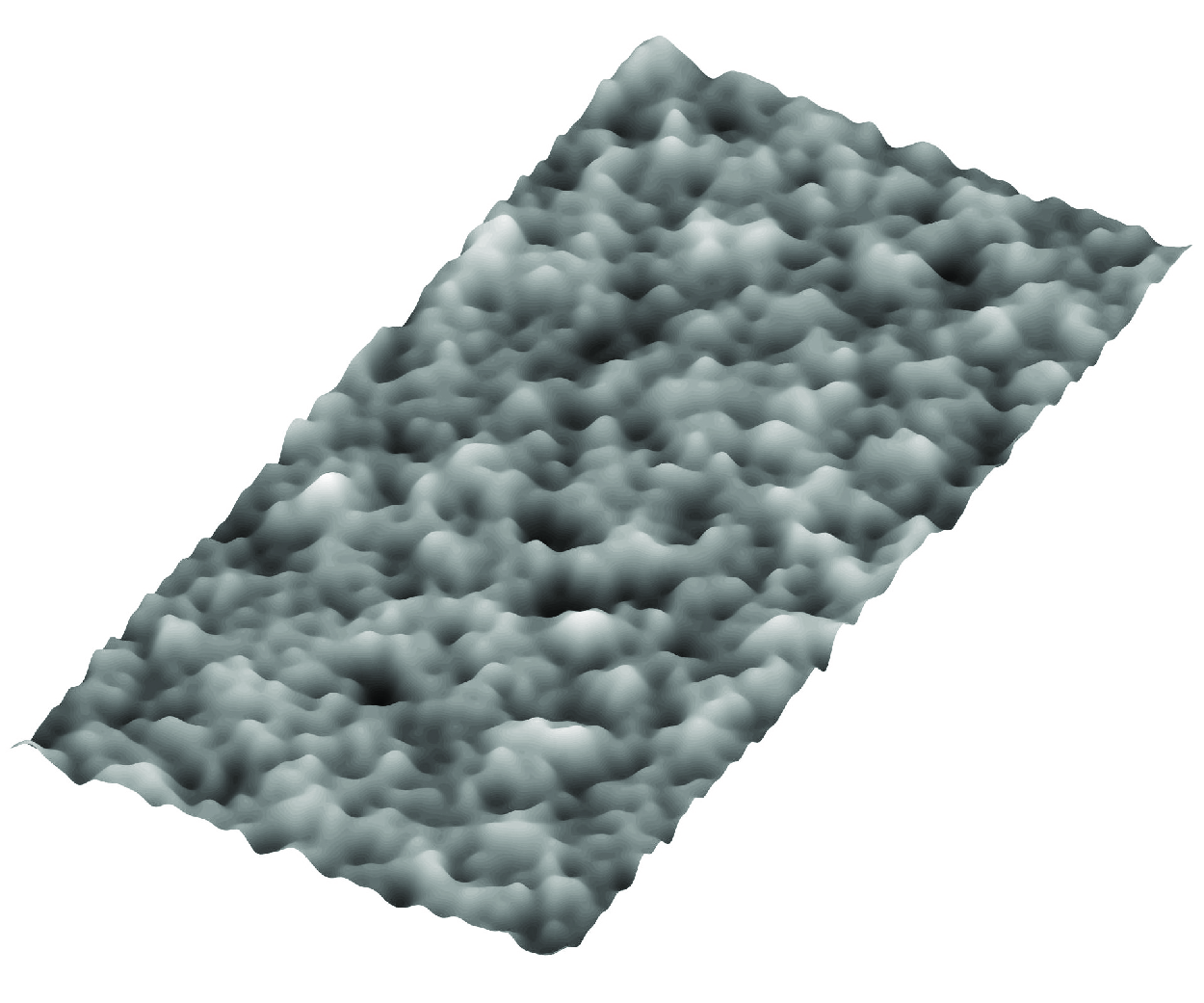
follow a Gaussian distribution so that the skewness of the rough surface approximately vanishes. As an example, figure 2 shows the surface roughness for the case
$\eta$
follow a Gaussian distribution so that the skewness of the rough surface approximately vanishes. As an example, figure 2 shows the surface roughness for the case
 $\rm C$
(see table 1) with
$\rm C$
(see table 1) with
 $k_{rms}=0.04$
.
$k_{rms}=0.04$
.

Figure 2. Example of a rough surface belonging to case C for
 $k_{rms}$
= 0.04.
$k_{rms}$
= 0.04.
The study was carried out by numerically solving the continuity and momentum equations. Using the friction velocity
 $u_{\tau }$
as the velocity scale and
$u_{\tau }$
as the velocity scale and
 $\varrho u_{\tau }^{2}$
as the pressure scale, where
$\varrho u_{\tau }^{2}$
as the pressure scale, where
 $\varrho$
is the fluid density, these equations take the following dimensionless form:
$\varrho$
is the fluid density, these equations take the following dimensionless form:
 \begin{align} \frac {\partial u_j}{\partial x_j}=0, \end{align}
 \begin{align} \frac {\partial u_i}{\partial t}+\frac {\partial u_i u_j}{\partial x_{j}}=-\frac {\partial p}{\partial x_i}+\frac {1}{R_{\tau }} \frac {\partial ^2 u_i}{\partial x_j \partial x_j}+\delta _{1,i},\end{align}
where
 $u_{i} (i = 1,2,3)$
are the velocity components (also referred to as
$u_{i} (i = 1,2,3)$
are the velocity components (also referred to as
 $u,v,w$
respectively),
$u,v,w$
respectively),
 $p$
is the pressure,
$p$
is the pressure,
 $R_{\tau }=u_{\tau }h/\nu$
is the Reynolds number, the subscripts
$R_{\tau }=u_{\tau }h/\nu$
is the Reynolds number, the subscripts
 $j$
= 1, 2 and 3 denote the directions
$j$
= 1, 2 and 3 denote the directions
 $x$
,
$x$
,
 $y$
and
$y$
and
 $z$
, respectively,
$z$
, respectively,
 $\delta _{1,i}$
is the Kronecker
$\delta _{1,i}$
is the Kronecker
 $\delta$
, and repeated subscripts are used to denote a summation. The numerical approach is based on centred second-order finite differences on a Cartesian staggered grid. The time advancement is based on a third-order Runge–Kutta method for the convective terms and on the Crank–Nicolson scheme for the viscous terms. Periodic boundary conditions are applied along the
$\delta$
, and repeated subscripts are used to denote a summation. The numerical approach is based on centred second-order finite differences on a Cartesian staggered grid. The time advancement is based on a third-order Runge–Kutta method for the convective terms and on the Crank–Nicolson scheme for the viscous terms. Periodic boundary conditions are applied along the
 $x$
and
$x$
and
 $z$
directions. On the bottom wall, the no-slip condition
$z$
directions. On the bottom wall, the no-slip condition
 $(u,v,w)=(0,0,0)$
is enforced, while on the top wall the free shear stress condition
$(u,v,w)=(0,0,0)$
is enforced, while on the top wall the free shear stress condition
 $(\partial u/\partial y,v, \partial w/\partial y)=(0,0,0)$
is enforced as in Yuan & Piomelli (Reference Yuan and Piomelli2014b
). The boundary condition on the bottom rough surface is imposed by an immersed boundary method similar to that used by Leonardi et al. (Reference Leonardi, Orlandi, Smalley, Djenidi, Paden and Antonia2003).
$(\partial u/\partial y,v, \partial w/\partial y)=(0,0,0)$
is enforced as in Yuan & Piomelli (Reference Yuan and Piomelli2014b
). The boundary condition on the bottom rough surface is imposed by an immersed boundary method similar to that used by Leonardi et al. (Reference Leonardi, Orlandi, Smalley, Djenidi, Paden and Antonia2003).
In all simulations, the dimensionless lengths of the fluid domain
 $L_{x}$
and
$L_{x}$
and
 $L_{z}$
are set to 6 and 3, respectively, and the Reynolds number
$L_{z}$
are set to 6 and 3, respectively, and the Reynolds number
 $R_{\tau }$
is set to 500. The size of the numerical grid
$R_{\tau }$
is set to 500. The size of the numerical grid
 $(n_{x},n_{y},n_{z})$
varied from (300, 220, 300) to (480, 400, 360) as shown more in detail in tables 2–6 in Appendix A. The grid spacing in the
$(n_{x},n_{y},n_{z})$
varied from (300, 220, 300) to (480, 400, 360) as shown more in detail in tables 2–6 in Appendix A. The grid spacing in the
 $x$
direction is smaller than or equal to 10 wall units. Spatial resolution of about 10 wall units in the
$x$
direction is smaller than or equal to 10 wall units. Spatial resolution of about 10 wall units in the
 $x$
direction has been used by Guo-Zhen et al. (Reference Guo-Zhen, Chun-Xiao, Hyung and Wei-Xi2020) who used a spacing of 11 wall units in the
$x$
direction has been used by Guo-Zhen et al. (Reference Guo-Zhen, Chun-Xiao, Hyung and Wei-Xi2020) who used a spacing of 11 wall units in the
 $x$
direction. A spacing of 8–10 wall units in the flow direction has been used with the present code to study oscillatory flow on an irregular rough bed in Dunbar et al. (Reference Dunbar, Van Der, Scandura and O’Donoghue2023). In that study, the DNS results were compared with experimental measurements using a laser Doppler anemometer in a large oscillating flow tunnel, with good agreement even for the higher-order statistics of the velocity fluctuations. The spatial resolution in the flow direction is 6 wall units with 480 meshes in the
$x$
direction. A spacing of 8–10 wall units in the flow direction has been used with the present code to study oscillatory flow on an irregular rough bed in Dunbar et al. (Reference Dunbar, Van Der, Scandura and O’Donoghue2023). In that study, the DNS results were compared with experimental measurements using a laser Doppler anemometer in a large oscillating flow tunnel, with good agreement even for the higher-order statistics of the velocity fluctuations. The spatial resolution in the flow direction is 6 wall units with 480 meshes in the
 $x$
direction for the simulations of case E, which has the highest wavenumbers, corresponding to 7 grid points at the shortest wavelength. Regarding the grid convergence, for example, in case E, for
$x$
direction for the simulations of case E, which has the highest wavenumbers, corresponding to 7 grid points at the shortest wavelength. Regarding the grid convergence, for example, in case E, for
 $k_{rms}=0.075$
, increasing the number of grid points in the
$k_{rms}=0.075$
, increasing the number of grid points in the
 $x$
direction from 360 to 480, the variation of
$x$
direction from 360 to 480, the variation of
 $\Delta U^{+}$
was less than 0.1 over a
$\Delta U^{+}$
was less than 0.1 over a
 $\Delta U^{+}$
of about 10.8, which is less than 1 %.
$\Delta U^{+}$
of about 10.8, which is less than 1 %.
The grid spacing in the
 $y$
direction is not constant, as a number of grid points are clustered near the rough surface, where large gradients exist. More specifically, in the layer between the lowest trough and the highest peak of the roughness, the grid spacing
$y$
direction is not constant, as a number of grid points are clustered near the rough surface, where large gradients exist. More specifically, in the layer between the lowest trough and the highest peak of the roughness, the grid spacing
 $\Delta y^{+}$
was kept below 1.
$\Delta y^{+}$
was kept below 1.
3. Discussion of the results
The roughness function was determined by fitting the logarithmic law of the wall, expressed by the (3.1), to the spatial and temporal average of the streamwise velocity data:
 \begin{equation} u^+=\frac {1}{k} \log (y^+-d^+)+C-\Delta U^+. \end{equation}
In (3.1),
 $k=0.4$
is the von Kármán constant,
$k=0.4$
is the von Kármán constant,
 $C=5$
is a constant and
$C=5$
is a constant and
 $d^+$
is a shift away from the plane
$d^+$
is a shift away from the plane
 $y^{+}=0$
to maximise the quality of the logarithmic fit. The values of
$y^{+}=0$
to maximise the quality of the logarithmic fit. The values of
 $d^+$
and
$d^+$
and
 $\Delta U^+$
were estimated by the least squares method in the interval
$\Delta U^+$
were estimated by the least squares method in the interval
 $40 \leqslant (y^+-d^+) \leqslant 150$
. To check the sensitivity of
$40 \leqslant (y^+-d^+) \leqslant 150$
. To check the sensitivity of
 $\Delta U^{+}$
to the interval used, increasing the lower bound to 50 resulted in a difference of less than 0.1. A similar range was considered by Forooghi et al. (Reference Forooghi, Stroh, Magagnato, Jakirlic and Frohnapfel2017) who used
$\Delta U^{+}$
to the interval used, increasing the lower bound to 50 resulted in a difference of less than 0.1. A similar range was considered by Forooghi et al. (Reference Forooghi, Stroh, Magagnato, Jakirlic and Frohnapfel2017) who used
 $y^{+}=30$
as the lower bound and
$y^{+}=30$
as the lower bound and
 $y/h$
= 0.3 as the upper bound. In Appendix A, tables 2–6 show the parameters of the rough surfaces and the numerical values of
$y/h$
= 0.3 as the upper bound. In Appendix A, tables 2–6 show the parameters of the rough surfaces and the numerical values of
 $\Delta U^{+}$
.
$\Delta U^{+}$
.
Figure 3(a) shows some semi-logarithmic plots of the velocity profiles for case E, from which it is evident that the velocity decreases as
 $k_{rms}$
increases.
$k_{rms}$
increases.

Figure 3. (a) Semi-logarithmic plot of the velocity profiles for case E. (b) Velocity defect profiles for case E.
As shown in tables 2–6, some of the rough surfaces are characterised by a relatively large
 $S_{y5\times 5}$
(Thakkar et al. Reference Thakkar, Busse and Sandham2017), which may hinder the similarity of velocity profiles normally observed outside the region directly affected by the roughness. Figure 3(b) shows the velocity defect profiles for case E, which is that characterised by the largest roughness heights. It can be seen that the velocity defect profiles approximately follow the trend of the smooth-wall case with some larger deviations for
$S_{y5\times 5}$
(Thakkar et al. Reference Thakkar, Busse and Sandham2017), which may hinder the similarity of velocity profiles normally observed outside the region directly affected by the roughness. Figure 3(b) shows the velocity defect profiles for case E, which is that characterised by the largest roughness heights. It can be seen that the velocity defect profiles approximately follow the trend of the smooth-wall case with some larger deviations for
 $k_{rms}=0.085$
. To explain why, despite the large
$k_{rms}=0.085$
. To explain why, despite the large
 $S_{y5\times 5}$
, there is still a similarity between the velocity profiles of the smooth- and rough-wall cases, a new measure of roughness height, called
$S_{y5\times 5}$
, there is still a similarity between the velocity profiles of the smooth- and rough-wall cases, a new measure of roughness height, called
 $H_{5\, \%5\times 5}$
, is introduced. This height is based on the difference between the position
$H_{5\, \%5\times 5}$
, is introduced. This height is based on the difference between the position
 $y_u$
, above which the roughness covers less than 5 % of the total surface x–z, and
$y_u$
, above which the roughness covers less than 5 % of the total surface x–z, and
 $y_l$
, below which the fluid covers less than 5 % of the total surface. Height
$y_l$
, below which the fluid covers less than 5 % of the total surface. Height
 $H_{5\, \%5\times 5}$
is determined as
$H_{5\, \%5\times 5}$
is determined as
 $S_{y5\times 5}$
, i.e. the surface is divided into
$S_{y5\times 5}$
, i.e. the surface is divided into
 $5 \times 5$
tiles and for each of these
$5 \times 5$
tiles and for each of these
 $y_u$
and
$y_u$
and
 $y_l$
are determined. Finally,
$y_l$
are determined. Finally,
 $H_{5\, \%5\times 5}$
is calculated as the arithmetic mean of
$H_{5\, \%5\times 5}$
is calculated as the arithmetic mean of
 $y_u-y_l$
of all the tiles. It can be observed that
$y_u-y_l$
of all the tiles. It can be observed that
 $S_{y5\times 5}$
is obtained as the special case when the percentage is set to zero. The reason for introducing this measure of roughness height is that for the roughness to break the similarity of the velocity profiles, it is not enough for its height to be large; the roughness must also cover a sufficiently large proportion of the total area. The value of
$S_{y5\times 5}$
is obtained as the special case when the percentage is set to zero. The reason for introducing this measure of roughness height is that for the roughness to break the similarity of the velocity profiles, it is not enough for its height to be large; the roughness must also cover a sufficiently large proportion of the total area. The value of
 $5\, \%$
of the total area is chosen as the value below which it seems reasonable that the roughness will not have a significant effect on the velocity defect profiles. In tables 2–6 it can be seen that
$5\, \%$
of the total area is chosen as the value below which it seems reasonable that the roughness will not have a significant effect on the velocity defect profiles. In tables 2–6 it can be seen that
 $H_{5\, \%5\times 5}$
is about half of
$H_{5\, \%5\times 5}$
is about half of
 $S_{y5 \times 5}$
, which can explain why the similarity of the velocity profiles is maintained. As a further check on the effect of roughness height, the mean velocity profiles were also computed using the intrinsic spatial average (average over the fluid domain only) and for case
$S_{y5 \times 5}$
, which can explain why the similarity of the velocity profiles is maintained. As a further check on the effect of roughness height, the mean velocity profiles were also computed using the intrinsic spatial average (average over the fluid domain only) and for case
 ${\rm E}_{10}$
the difference in
${\rm E}_{10}$
the difference in
 $\Delta U^{+}$
with respect to the spatial average was only about 0.3 %.
$\Delta U^{+}$
with respect to the spatial average was only about 0.3 %.

Figure 4. (a) Roughness function versus
 $k_{rms}^{+}$
. Here SF 2009a and SF 2009b refer to the data of Schultz & Flack (Reference Schultz and Flack2009) for
$k_{rms}^{+}$
. Here SF 2009a and SF 2009b refer to the data of Schultz & Flack (Reference Schultz and Flack2009) for
 $\alpha =45^\circ$
and
$\alpha =45^\circ$
and
 $\alpha =22^\circ$
, respectively. The dashed curve is described by the equation
$\alpha =22^\circ$
, respectively. The dashed curve is described by the equation
 $(1/k)\log(k_{rms}^{+})+1.76$
. (b) roughness function versus
$(1/k)\log(k_{rms}^{+})+1.76$
. (b) roughness function versus
 $ES$
. Here SF 2009c1,c2,c3 refer to the highest-Reynolds-number cases of Schultz & Flack (Reference Schultz and Flack2009) for
$ES$
. Here SF 2009c1,c2,c3 refer to the highest-Reynolds-number cases of Schultz & Flack (Reference Schultz and Flack2009) for
 $\alpha =11^\circ$
.
$\alpha =11^\circ$
.
In figure 4(a), where
 $\Delta U^{+}$
is plotted against
$\Delta U^{+}$
is plotted against
 $k_{rms}$
for cases A–E, it can be seen that
$k_{rms}$
for cases A–E, it can be seen that
 $\Delta U^{+}$
scales with
$\Delta U^{+}$
scales with
 $k_{rms}$
only within each case, highlighting that the roughness function is influenced by additional surface properties depending on the PSD. As we move from case A to case E, for a fixed
$k_{rms}$
only within each case, highlighting that the roughness function is influenced by additional surface properties depending on the PSD. As we move from case A to case E, for a fixed
 $k_{rms}$
,
$k_{rms}$
,
 $\Delta U^{+}$
increases first rapidly and then slowly, so there is not much difference between cases D and E, which are characterised by the largest wavenumbers. For comparison, figure 4(a) also shows data from Schultz & Flack (Reference Schultz and Flack2009), who performed experiments with a rough wall made of square-based pyramids, considering three different cases of the angle of inclination
$\Delta U^{+}$
increases first rapidly and then slowly, so there is not much difference between cases D and E, which are characterised by the largest wavenumbers. For comparison, figure 4(a) also shows data from Schultz & Flack (Reference Schultz and Flack2009), who performed experiments with a rough wall made of square-based pyramids, considering three different cases of the angle of inclination
 $\alpha$
of the pyramid diagonal:
$\alpha$
of the pyramid diagonal:
 $45^\circ$
,
$45^\circ$
,
 $22^\circ$
and
$22^\circ$
and
 $11^\circ$
. Figure 4(a) shows only the data for
$11^\circ$
. Figure 4(a) shows only the data for
 $\alpha$
equal to
$\alpha$
equal to
 $45^\circ$
and
$45^\circ$
and
 $22^\circ$
as a function of
$22^\circ$
as a function of
 $k_{rms}^{+}$
, determined as
$k_{rms}^{+}$
, determined as
 $k_{rms}^{+}=k_{t}^{+}/\sqrt {18}$
, where
$k_{rms}^{+}=k_{t}^{+}/\sqrt {18}$
, where
 $k_{t}^{+}$
is the height of the pyramid. When comparing the two datasets, it should be noted that in the present study
$k_{t}^{+}$
is the height of the pyramid. When comparing the two datasets, it should be noted that in the present study
 $ES$
changes as
$ES$
changes as
 $k_{rms}^{+}$
increases, whereas in Schultz & Flack (Reference Schultz and Flack2009)
$k_{rms}^{+}$
increases, whereas in Schultz & Flack (Reference Schultz and Flack2009)
 $ES$
is held constant and is equal to 1 for
$ES$
is held constant and is equal to 1 for
 $\alpha =45^\circ$
and 0.40 for
$\alpha =45^\circ$
and 0.40 for
 $\alpha =22^\circ$
. We note that despite the large difference in
$\alpha =22^\circ$
. We note that despite the large difference in
 $\alpha$
between SF 2009a and SF 2009b, these experimental data show no clear difference between them. On the other hand, the present results show a gap in
$\alpha$
between SF 2009a and SF 2009b, these experimental data show no clear difference between them. On the other hand, the present results show a gap in
 $\Delta U^{+}$
between the different power spectra, albeit small in some cases. Nevertheless, the present results show a trend that is in line with that of Schultz & Flack (Reference Schultz and Flack2009), especially for cases D and E, and the relatively small differences can be explained by the different values of
$\Delta U^{+}$
between the different power spectra, albeit small in some cases. Nevertheless, the present results show a trend that is in line with that of Schultz & Flack (Reference Schultz and Flack2009), especially for cases D and E, and the relatively small differences can be explained by the different values of
 $ES$
, as described below. For case E, in the interval
$ES$
, as described below. For case E, in the interval
 $k_{rms}^{+}=2.5{-}10$
, the effective slope ranges from 0 to 0.4, i.e. it is smaller than that of Schultz & Flack (Reference Schultz and Flack2009) (0.4–1), so that the present
$k_{rms}^{+}=2.5{-}10$
, the effective slope ranges from 0 to 0.4, i.e. it is smaller than that of Schultz & Flack (Reference Schultz and Flack2009) (0.4–1), so that the present
 $\Delta U^{+}$
is generally smaller than that of the aforementioned study. In the range
$\Delta U^{+}$
is generally smaller than that of the aforementioned study. In the range
 $k_{rms}^{+}=10{-}25$
, the present values of
$k_{rms}^{+}=10{-}25$
, the present values of
 $ES$
vary approximately between 0.4 and 1, then the effective slopes are similar and we find that the two
$ES$
vary approximately between 0.4 and 1, then the effective slopes are similar and we find that the two
 $\Delta U^{+}$
are also similar. Finally, for
$\Delta U^{+}$
are also similar. Finally, for
 $k_{rms}^{+}\gt 25$
the present effective slope is larger than that of Schultz & Flack (Reference Schultz and Flack2009), and hence the present
$k_{rms}^{+}\gt 25$
the present effective slope is larger than that of Schultz & Flack (Reference Schultz and Flack2009), and hence the present
 $\Delta U^{+}$
are larger than those of the aforementioned study. This comparison shows that the present results are generally consistent with those of Schultz & Flack (Reference Schultz and Flack2009), even from a quantitative point of view.
$\Delta U^{+}$
are larger than those of the aforementioned study. This comparison shows that the present results are generally consistent with those of Schultz & Flack (Reference Schultz and Flack2009), even from a quantitative point of view.
As shown in figure 4(b), even when
 $\Delta U^{+}$
is plotted against the effective slope
$\Delta U^{+}$
is plotted against the effective slope
 $ES$
, the data collapse on the same curve only within each case. This result contrasts with that of Napoli et al. (Reference Napoli, Armenio and De Marchis2008), also shown in figure 4(b), who obtained data collapse on the same curve regardless of the roughness amplitude.
$ES$
, the data collapse on the same curve only within each case. This result contrasts with that of Napoli et al. (Reference Napoli, Armenio and De Marchis2008), also shown in figure 4(b), who obtained data collapse on the same curve regardless of the roughness amplitude.
Figure 4(a) shows that cases A and B are quite far apart, whereas in figure 4(b) they are very close to each other and together they are also close to most of the data from Napoli et al. (Reference Napoli, Armenio and De Marchis2008). Therefore, based on cases A and B, one could conclude that
 $\Delta U^{+}$
scales with
$\Delta U^{+}$
scales with
 $ES$
. This shows that a possible explanation for
$ES$
. This shows that a possible explanation for
 $\Delta U^{+}$
scaling with
$\Delta U^{+}$
scaling with
 $ES$
in Napoli et al. (Reference Napoli, Armenio and De Marchis2008) could be the use of surface roughness with a power density spectrum characterised by small wavenumbers, as in cases A and B. If only surface roughness with power density spectra characterised by very high wavenumbers is considered, as in cases D and E, different conclusions can be drawn. In fact, as figure 4(a) shows, the data from cases D and E appear very close to each other when plotted against
$ES$
in Napoli et al. (Reference Napoli, Armenio and De Marchis2008) could be the use of surface roughness with a power density spectrum characterised by small wavenumbers, as in cases A and B. If only surface roughness with power density spectra characterised by very high wavenumbers is considered, as in cases D and E, different conclusions can be drawn. In fact, as figure 4(a) shows, the data from cases D and E appear very close to each other when plotted against
 $k_{rms}^{+}$
, so one could claim that in general
$k_{rms}^{+}$
, so one could claim that in general
 $\Delta U^+$
scales with
$\Delta U^+$
scales with
 $k_{rms}^{+}$
, which is clearly not true when looking at the overall picture of the results.
$k_{rms}^{+}$
, which is clearly not true when looking at the overall picture of the results.
Since the data from Schultz & Flack (Reference Schultz and Flack2009) shown in figure 4(a) scale with
 $k_{rms}^{+}$
, it is expected the rough surface is also characterised by large wavenumbers. Taking the wavenumber relative to the diagonal of the pyramid used as the roughness element as the reference wavenumber and scaling it by the thickness of the boundary layer, the wavenumbers range from 64 to 294 for
$k_{rms}^{+}$
, it is expected the rough surface is also characterised by large wavenumbers. Taking the wavenumber relative to the diagonal of the pyramid used as the roughness element as the reference wavenumber and scaling it by the thickness of the boundary layer, the wavenumbers range from 64 to 294 for
 $\alpha =45^\circ$
and
$\alpha =45^\circ$
and
 $\alpha =22^\circ$
and from 31 to 53 for
$\alpha =22^\circ$
and from 31 to 53 for
 $\alpha =11^\circ$
. Again, this result shows that scaling with roughness height is associated with high wavenumbers. Indeed, the case with
$\alpha =11^\circ$
. Again, this result shows that scaling with roughness height is associated with high wavenumbers. Indeed, the case with
 $\alpha =11^\circ$
did not scale with either
$\alpha =11^\circ$
did not scale with either
 $k_{rms}$
or
$k_{rms}$
or
 $ES$
. The term ’waviness’ regime was introduced by the authors for this case to indicate flows on surfaces with long wavelengths where
$ES$
. The term ’waviness’ regime was introduced by the authors for this case to indicate flows on surfaces with long wavelengths where
 $\Delta U^{+}$
does not scale with roughness height. However, the effect of the wavenumber is also clearly visible within the data with
$\Delta U^{+}$
does not scale with roughness height. However, the effect of the wavenumber is also clearly visible within the data with
 $\alpha =11^\circ$
. In fact, the case
$\alpha =11^\circ$
. In fact, the case
 $\alpha =11^\circ$
consists of three subsets of data, each characterised by an approximately constant wavenumber, and it can be seen that within each of these subsets,
$\alpha =11^\circ$
consists of three subsets of data, each characterised by an approximately constant wavenumber, and it can be seen that within each of these subsets,
 $\Delta U^{+}$
scales with
$\Delta U^{+}$
scales with
 $k_{rms}^{+}$
. Among these three cases, that characterised by the largest wavenumber has the largest
$k_{rms}^{+}$
. Among these three cases, that characterised by the largest wavenumber has the largest
 $\Delta U^{+}$
for a given roughness size (see figure 11 of Schultz & Flack (Reference Schultz and Flack2009)). The values of
$\Delta U^{+}$
for a given roughness size (see figure 11 of Schultz & Flack (Reference Schultz and Flack2009)). The values of
 $\Delta U^{+}$
obtained for the largest Reynolds numbers from these three subsets are shown in figure 4(b) and it can be seen that they are close to the present results obtained for the surface characterised by low wavenumbers.
$\Delta U^{+}$
obtained for the largest Reynolds numbers from these three subsets are shown in figure 4(b) and it can be seen that they are close to the present results obtained for the surface characterised by low wavenumbers.
In general, the rate of increase of
 $\Delta U^{+}$
with
$\Delta U^{+}$
with
 $k_{rms}^{+}$
tends to decrease as this quantity increases (note that
$k_{rms}^{+}$
tends to decrease as this quantity increases (note that
 $ES$
also increases with
$ES$
also increases with
 $k_{rms}^{+}$
). This is because the increase in
$k_{rms}^{+}$
). This is because the increase in
 $k_{rms}^{+}$
causes an increase in
$k_{rms}^{+}$
causes an increase in
 $S_{y5\times 5}$
resulting in deep depressions where the flow has recirculation zones enclosed between ridges with little interaction with the external flow. In these cases, only the upper part of the roughness makes a significant contribution to drag, and a further increase in
$S_{y5\times 5}$
resulting in deep depressions where the flow has recirculation zones enclosed between ridges with little interaction with the external flow. In these cases, only the upper part of the roughness makes a significant contribution to drag, and a further increase in
 $k_{rms}$
will not result in a significant increase in
$k_{rms}$
will not result in a significant increase in
 $\Delta U^{+}$
. This behaviour is related to the asymptotic tendency of
$\Delta U^{+}$
. This behaviour is related to the asymptotic tendency of
 $\Delta U^{+}$
towards the logarithm of
$\Delta U^{+}$
towards the logarithm of
 $k_{rms}^{+}$
, typical of flows approaching the fully rough regime. In the case of the Nikuradse sand roughness, reaching the fully rough regime is indicated by the roughness function varying according to the equation
$k_{rms}^{+}$
, typical of flows approaching the fully rough regime. In the case of the Nikuradse sand roughness, reaching the fully rough regime is indicated by the roughness function varying according to the equation
 \begin{eqnarray} \Delta U^{+}=\frac {1}{k }\log\left (k_{s}^{+}\right )+a, \end{eqnarray}
with
 $a =-3.5$
. If
$a =-3.5$
. If
 $k_{rms}$
is used instead of
$k_{rms}$
is used instead of
 $k_{s}$
, the roughness function in the fully rough regime still obeys an equation similar to (3.2) where
$k_{s}$
, the roughness function in the fully rough regime still obeys an equation similar to (3.2) where
 $k_{s}^{+}$
is replaced by
$k_{s}^{+}$
is replaced by
 $k_{rms}^{+}$
and
$k_{rms}^{+}$
and
 $a$
takes a different value from that given above.
$a$
takes a different value from that given above.
In figure 4(a) it can be seen that as
 $k_{rms}^{+}$
increases, the curves tend to converge, and it appears that overall they tend to converge towards the curve of (3.2) with
$k_{rms}^{+}$
increases, the curves tend to converge, and it appears that overall they tend to converge towards the curve of (3.2) with
 $a=1.76$
and
$a=1.76$
and
 $k_{s}^{+}$
replaced by
$k_{s}^{+}$
replaced by
 $k_{rms}^{+}$
(see the dashed line in figure 4(a)). Since for a fixed value of
$k_{rms}^{+}$
(see the dashed line in figure 4(a)). Since for a fixed value of
 $k_{rms}^{+}$
each curve is characterised by a different value of
$k_{rms}^{+}$
each curve is characterised by a different value of
 $ES$
, and yet the curves become closer and closer together, it follows that
$ES$
, and yet the curves become closer and closer together, it follows that
 $ES$
does not affect the behaviour of the curves for large
$ES$
does not affect the behaviour of the curves for large
 $k_{rms}^{+}$
. This is because as
$k_{rms}^{+}$
. This is because as
 $k_{rms}^{+}$
increases, so does
$k_{rms}^{+}$
increases, so does
 $ES$
, and at some point
$ES$
, and at some point
 $\Delta U^{+}$
saturates with respect to
$\Delta U^{+}$
saturates with respect to
 $ES$
, after which
$ES$
, after which
 $\Delta U^{+}$
starts to scale only with
$\Delta U^{+}$
starts to scale only with
 $k_{rms}^{+}$
. This is consistent with the statement of Schultz & Flack (Reference Schultz and Flack2009) that if the roughness slope is steep enough, the roughness function will scale completely to the roughness height.
$k_{rms}^{+}$
. This is consistent with the statement of Schultz & Flack (Reference Schultz and Flack2009) that if the roughness slope is steep enough, the roughness function will scale completely to the roughness height.
To provide a further proof of the independence of
 $\Delta U^{+}$
on
$\Delta U^{+}$
on
 $ES$
, we focus on case E to prove by a test that
$ES$
, we focus on case E to prove by a test that
 $\Delta U^{+}$
scales with
$\Delta U^{+}$
scales with
 $k_{rms}^{+}$
for large values of this variable. To perform this test, the rough surface of case
$k_{rms}^{+}$
for large values of this variable. To perform this test, the rough surface of case
 ${\rm E}_8$
(
${\rm E}_8$
(
 $k_{rms}=0.065$
) was used to perform an additional simulation with
$k_{rms}=0.065$
) was used to perform an additional simulation with
 $R_{\tau }=654$
which gives
$R_{\tau }=654$
which gives
 $k_{rms}^{+}=42.5$
. This new simulation has the same
$k_{rms}^{+}=42.5$
. This new simulation has the same
 $k_{rms}^{+}$
as that of case
$k_{rms}^{+}$
as that of case
 ${\rm E}_{10}$
at
${\rm E}_{10}$
at
 $R_{\tau }=500$
(
$R_{\tau }=500$
(
 $k_{rms}=0.085$
,
$k_{rms}=0.085$
,
 $k_{rms}^{+}=42.5$
) but
$k_{rms}^{+}=42.5$
) but
 $ES$
of case
$ES$
of case
 ${\rm E}_8$
. By comparing the result of this simulation with that of case
${\rm E}_8$
. By comparing the result of this simulation with that of case
 ${\rm E}_{10}$
it can be verified if
${\rm E}_{10}$
it can be verified if
 $\Delta U^{+}$
scales only with
$\Delta U^{+}$
scales only with
 $k_{rms}^{+}$
or if there is also an influence of
$k_{rms}^{+}$
or if there is also an influence of
 $ES$
. The result of this additional simulation shows that for
$ES$
. The result of this additional simulation shows that for
 $k_{rms}=0.065$
and
$k_{rms}=0.065$
and
 $R_{\tau }=654$
the roughness function takes a value of 11.16, while for
$R_{\tau }=654$
the roughness function takes a value of 11.16, while for
 $k_{rms}=0.085$
and
$k_{rms}=0.085$
and
 $R_{\tau }=500$
a value of 11.14 was obtained. The difference in
$R_{\tau }=500$
a value of 11.14 was obtained. The difference in
 $\Delta U^{+}$
is about 0.2 % and is very small considering that it results from a difference in
$\Delta U^{+}$
is about 0.2 % and is very small considering that it results from a difference in
 $ES$
of 30 %. This shows that
$ES$
of 30 %. This shows that
 $\Delta U^{+}$
scales with
$\Delta U^{+}$
scales with
 $k_{rms}^{+}$
. This result is only valid for case E; for the other cases shown in table 1, a test like the previous one would have shown a dependence of
$k_{rms}^{+}$
. This result is only valid for case E; for the other cases shown in table 1, a test like the previous one would have shown a dependence of
 $\Delta U^{+}$
on
$\Delta U^{+}$
on
 $ES$
especially for cases A and B.
$ES$
especially for cases A and B.
Many studies have shown that for a fixed value of roughness height,
 $\Delta U^{+}$
increases for
$\Delta U^{+}$
increases for
 $ES$
less than a certain value, reaches a maximum and then decreases as
$ES$
less than a certain value, reaches a maximum and then decreases as
 $ES$
is further increased. This decrease in
$ES$
is further increased. This decrease in
 $\Delta U^{+}$
occurs because for large
$\Delta U^{+}$
occurs because for large
 $ES$
the roughness enters the dense regime, where the roughness elements shelter each other from the flow. This may lead to the conclusion that the previously shown independence of
$ES$
the roughness enters the dense regime, where the roughness elements shelter each other from the flow. This may lead to the conclusion that the previously shown independence of
 $\Delta U^{+}$
from
$\Delta U^{+}$
from
 $ES$
in the interval
$ES$
in the interval
 $k_{rms}=0.065{-}0.085$
is merely a consequence of
$k_{rms}=0.065{-}0.085$
is merely a consequence of
 $\Delta U^{+}$
being close to its maximum, so that if
$\Delta U^{+}$
being close to its maximum, so that if
 $k_{rms}$
is increased further, the dependence on
$k_{rms}$
is increased further, the dependence on
 $ES$
could emerge and cause the deviation of
$ES$
could emerge and cause the deviation of
 $\Delta U^{+}$
from the fully rough asymptote. In this regard, note that as
$\Delta U^{+}$
from the fully rough asymptote. In this regard, note that as
 $k_{rms}$
increases, the wavenumbers of the rough surface remain unchanged, as the shape of the power density spectrum is constant for each of the cases shown in table 1. Therefore, the roughness does not become more densely packed and no decrease in
$k_{rms}$
increases, the wavenumbers of the rough surface remain unchanged, as the shape of the power density spectrum is constant for each of the cases shown in table 1. Therefore, the roughness does not become more densely packed and no decrease in
 $\Delta U^{+}$
with
$\Delta U^{+}$
with
 $ES$
is observed. An example where an increase in
$ES$
is observed. An example where an increase in
 $ES$
led to a decrease in
$ES$
led to a decrease in
 $\Delta U^{+}$
can be found in MacDonald et al. (Reference MacDonald, Chan, Chung, Hutchings and Ooi2016), where the roughness height was kept constant and the increase in
$\Delta U^{+}$
can be found in MacDonald et al. (Reference MacDonald, Chan, Chung, Hutchings and Ooi2016), where the roughness height was kept constant and the increase in
 $ES$
was obtained by decreasing the roughness wavelength. Those authors showed that
$ES$
was obtained by decreasing the roughness wavelength. Those authors showed that
 $\Delta U^{+}$
peaks at about
$\Delta U^{+}$
peaks at about
 $ES=2 \varLambda \approx 0.3$
(see also figure 5a in Chung et al. (Reference Chung, Hutchings, Schultz and Flack2021)) and then decreases with
$ES=2 \varLambda \approx 0.3$
(see also figure 5a in Chung et al. (Reference Chung, Hutchings, Schultz and Flack2021)) and then decreases with
 $ES$
. Further support for the hypothesis of independence of
$ES$
. Further support for the hypothesis of independence of
 $\Delta U^{+}$
from
$\Delta U^{+}$
from
 $ES$
comes from previous studies which, in the case of irregular rough surfaces, have shown a monotonic increase of
$ES$
comes from previous studies which, in the case of irregular rough surfaces, have shown a monotonic increase of
 $\Delta U^{+}$
with
$\Delta U^{+}$
with
 $ES$
for a fixed roughness height, with a tendency to reach a plateau at large
$ES$
for a fixed roughness height, with a tendency to reach a plateau at large
 $ES$
(Yuan & Piomelli Reference Yuan and Piomelli2014
a; Kuwata & Nagura Reference Kuwata and Nagura2020). This behaviour is also observed in the present case, as can be seen in the figure 6, which is discussed in the following. This result, combined with the constancy of the shape of the PSD, gives confidence that as
$ES$
(Yuan & Piomelli Reference Yuan and Piomelli2014
a; Kuwata & Nagura Reference Kuwata and Nagura2020). This behaviour is also observed in the present case, as can be seen in the figure 6, which is discussed in the following. This result, combined with the constancy of the shape of the PSD, gives confidence that as
 $k_{rms}$
increases,
$k_{rms}$
increases,
 $\Delta U^{+}$
is unaffected by
$\Delta U^{+}$
is unaffected by
 $ES$
for large effective slopes. Despite the above evidence for the independence of
$ES$
for large effective slopes. Despite the above evidence for the independence of
 $\Delta U^{+}$
from
$\Delta U^{+}$
from
 $ES$
, it is possible to further verify it for
$ES$
, it is possible to further verify it for
 $k_{rms}$
larger than considered here by performing simulations for higher
$k_{rms}$
larger than considered here by performing simulations for higher
 $k_{rms}$
and larger Reynolds numbers. However, this is left to future studies on this topic.
$k_{rms}$
and larger Reynolds numbers. However, this is left to future studies on this topic.
Having shown that for large values of
 $ES$
the roughness function scales with
$ES$
the roughness function scales with
 $k_{rms}^{+}$
, it is possible to determine the equivalent sand roughness which, based on the previous discussion, is appropriate for large effective slopes such that
$k_{rms}^{+}$
, it is possible to determine the equivalent sand roughness which, based on the previous discussion, is appropriate for large effective slopes such that
 $\Delta U^{+}$
saturates when expressed as a function of
$\Delta U^{+}$
saturates when expressed as a function of
 $ES$
. The equivalent Nikuradse sand roughness can be calculated as
$ES$
. The equivalent Nikuradse sand roughness can be calculated as
 $k_{s}^{+}=\xi k_{rms}^{+}$
, where
$k_{s}^{+}=\xi k_{rms}^{+}$
, where
 $\xi =\exp[k (a+3.5)]$
and
$\xi =\exp[k (a+3.5)]$
and
 $a$
is the constant in equation (3.2) with
$a$
is the constant in equation (3.2) with
 $k_{s}^{+}$
replaced by
$k_{s}^{+}$
replaced by
 $k_{rms}^{+}$
as the independent variable. In figure 4
(a), the constant
$k_{rms}^{+}$
as the independent variable. In figure 4
(a), the constant
 $a$
of case E is about 1.76, so using the previous equation we get
$a$
of case E is about 1.76, so using the previous equation we get
 $\xi \approx 8.2$
. This value is very different from the
$\xi \approx 8.2$
. This value is very different from the
 $\xi =4.43$
reported by Flack & Schultz (Reference Flack and Schultz2010). Schultz & Flack (Reference Schultz and Flack2009), using their experimental data shown in the present figure 4
(a), obtained
$\xi =4.43$
reported by Flack & Schultz (Reference Flack and Schultz2010). Schultz & Flack (Reference Schultz and Flack2009), using their experimental data shown in the present figure 4
(a), obtained
 $k_{s}$
equal to 1.5 times the height of the pyramid. This relationship, expressed in terms of
$k_{s}$
equal to 1.5 times the height of the pyramid. This relationship, expressed in terms of
 $k_{rms}$
, becomes
$k_{rms}$
, becomes
 $k_{s}^{+}=6.36 k_{rms}^{+}$
which is still somewhat far from the current result. However, it should be noted that other studies have also found
$k_{s}^{+}=6.36 k_{rms}^{+}$
which is still somewhat far from the current result. However, it should be noted that other studies have also found
 $\xi$
to be approximately equal to 8. Based on a study of turbulent flow on a regular three-dimensional rough surface described by the product of two cosine waves of the type
$\xi$
to be approximately equal to 8. Based on a study of turbulent flow on a regular three-dimensional rough surface described by the product of two cosine waves of the type
 $\eta =A \cos(2\pi x/L_w) \cos(2\pi z/L_w)$
with wavelength
$\eta =A \cos(2\pi x/L_w) \cos(2\pi z/L_w)$
with wavelength
 $L_w$
, Guo-Zhen et al. (Reference Guo-Zhen, Chun-Xiao, Hyung and Wei-Xi2020) reported that in the fully rough regime
$L_w$
, Guo-Zhen et al. (Reference Guo-Zhen, Chun-Xiao, Hyung and Wei-Xi2020) reported that in the fully rough regime
 $k_{s}^{+}=3.7 A^+$
. Since
$k_{s}^{+}=3.7 A^+$
. Since
 $k_{rms}$
of this surface is equal to
$k_{rms}$
of this surface is equal to
 $0.5 A$
, we can write
$0.5 A$
, we can write
 $k_{s}^{+}=7.4 k_{rms}^{+}$
, which is not too far from the present result. Chan et al. (Reference Chan, MacDonald, Chung, Hutchins and Ooi2015) carried out a study of flow in a pipe made rough by sinusoidal undulations such as those described above and reported
$k_{s}^{+}=7.4 k_{rms}^{+}$
, which is not too far from the present result. Chan et al. (Reference Chan, MacDonald, Chung, Hutchins and Ooi2015) carried out a study of flow in a pipe made rough by sinusoidal undulations such as those described above and reported
 $k_{s}^{+}=4.1 A^{+}$
. This equation, when written in terms of
$k_{s}^{+}=4.1 A^{+}$
. This equation, when written in terms of
 $k_{rms}^{+}$
, reads as
$k_{rms}^{+}$
, reads as
 $k_{s}^{+}=8.2 k_{rms}^{+}$
, therefore consistent with the present result. The finding that for substantially different roughnesses, regular or irregular, the relationship between
$k_{s}^{+}=8.2 k_{rms}^{+}$
, therefore consistent with the present result. The finding that for substantially different roughnesses, regular or irregular, the relationship between
 $k_{rms}$
and
$k_{rms}$
and
 $k_{s}$
in the fully rough regime is expressed by a very similar relationship suggests that
$k_{s}$
in the fully rough regime is expressed by a very similar relationship suggests that
 $k_{rms}$
is an appropriate and fairly general measure of surface roughness.
$k_{rms}$
is an appropriate and fairly general measure of surface roughness.
An equation for the roughness function can also be provided for the transitional rough regime, but parameters in addition to
 $k_{rms}$
are required. The surface roughness considered in this study is characterised by three parameters,
$k_{rms}$
are required. The surface roughness considered in this study is characterised by three parameters,
 $k_{rms}$
,
$k_{rms}$
,
 $|\boldsymbol{\kappa}_{1c}|$
and
$|\boldsymbol{\kappa}_{1c}|$
and
 $|\boldsymbol{\kappa}_{2c}|$
, but as shown below, a good description of
$|\boldsymbol{\kappa}_{2c}|$
, but as shown below, a good description of
 $\Delta U^{+}$
can be obtained with only two parameters by replacing
$\Delta U^{+}$
can be obtained with only two parameters by replacing
 $|\boldsymbol{\kappa}_{1c}|$
and
$|\boldsymbol{\kappa}_{1c}|$
and
 $|\boldsymbol{\kappa}_{2c}|$
with
$|\boldsymbol{\kappa}_{2c}|$
with
 $ES$
. In fact, over a wide range of
$ES$
. In fact, over a wide range of
 $k_{rms}$
and
$k_{rms}$
and
 $ES$
, the roughness function can be approximately described by the equation
$ES$
, the roughness function can be approximately described by the equation
 \begin{eqnarray} \Delta U^{+}=\frac {1}{k} \log(k_{rms}^{+})+1.76-3.21 \exp(-3.51 ES) \nonumber \\ -0.42 k_{rms}^{+} \exp[-0.54 k_{rms}^{+} ES]. \end{eqnarray}
Equation (3.3) has four terms. The first term plus the second gives
 $\Delta U^{+}$
in the fully rough regime when
$\Delta U^{+}$
in the fully rough regime when
 $ES$
is large enough to cause the saturation of the roughness function. The third term provides a correction to the previous asymptote when
$ES$
is large enough to cause the saturation of the roughness function. The third term provides a correction to the previous asymptote when
 $ES$
does not take large values. Finally, the fourth term is introduced to reproduce the roughness function in the transitional rough regime. This term is therefore a measure of the deviation of the flow conditions from the fully rough regime. It should be noted that the region of very small
$ES$
does not take large values. Finally, the fourth term is introduced to reproduce the roughness function in the transitional rough regime. This term is therefore a measure of the deviation of the flow conditions from the fully rough regime. It should be noted that the region of very small
 $ES$
and large
$ES$
and large
 $k_{rms}^{+}$
was not explored in this study, so equation (3.3) is not reliable for these types of rough walls. The goodness of the fit of this equation to the numerical data can be seen in figure 5 and is evidenced by a coefficient of determination
$k_{rms}^{+}$
was not explored in this study, so equation (3.3) is not reliable for these types of rough walls. The goodness of the fit of this equation to the numerical data can be seen in figure 5 and is evidenced by a coefficient of determination
 $R^2 = 0.99$
. Given the good quality of the fit of (3.3) to the present data, it is worth presenting some plots of
$R^2 = 0.99$
. Given the good quality of the fit of (3.3) to the present data, it is worth presenting some plots of
 $\Delta U^{+}$
as a function of
$\Delta U^{+}$
as a function of
 $k_{rms}^{+}$
where
$k_{rms}^{+}$
where
 $ES$
is constant, and of
$ES$
is constant, and of
 $\Delta U^{+}$
as a function of
$\Delta U^{+}$
as a function of
 $ES$
where
$ES$
where
 $k_{rms}^{+}$
is constant, shown in figure 6. To be more reliable, these graphs have been drawn through the areas covered by numerical data. In figure 6(a) we observe that the larger
$k_{rms}^{+}$
is constant, shown in figure 6. To be more reliable, these graphs have been drawn through the areas covered by numerical data. In figure 6(a) we observe that the larger
 $ES$
the closer the curve is to the fully rough asymptote of case E and the earlier the fully rough regime is reached by increasing
$ES$
the closer the curve is to the fully rough asymptote of case E and the earlier the fully rough regime is reached by increasing
 $k_{rms}^{+}$
. In figure 6(b) we see that for a fixed value of
$k_{rms}^{+}$
. In figure 6(b) we see that for a fixed value of
 $k_{rms}^{+}$
, as the effective slope increases,
$k_{rms}^{+}$
, as the effective slope increases,
 $\Delta U^{+}$
also increases, but it reaches a plateau at about
$\Delta U^{+}$
also increases, but it reaches a plateau at about
 $ES=0.75$
, a result that can also be seen in figure 5.
$ES=0.75$
, a result that can also be seen in figure 5.


This picture differs from many studies which report that for a fixed roughness height
 $\Delta U^{+}$
reaches a maximum at
$\Delta U^{+}$
reaches a maximum at
 $ES \approx 0.3$
and then decreases with
$ES \approx 0.3$
and then decreases with
 $ES$
. However, the present results are consistent with those of other studies (Yuan & Piomelli Reference Yuan and Piomelli2014
a; Kuwata & Nagura Reference Kuwata and Nagura2020) on flows over an irregular rough surface. Therefore, this behaviour can be considered as a characteristic specific to irregular rough surfaces. A critical value of
$ES$
. However, the present results are consistent with those of other studies (Yuan & Piomelli Reference Yuan and Piomelli2014
a; Kuwata & Nagura Reference Kuwata and Nagura2020) on flows over an irregular rough surface. Therefore, this behaviour can be considered as a characteristic specific to irregular rough surfaces. A critical value of
 $ES$
for irregular rough surfaces, above which
$ES$
for irregular rough surfaces, above which
 $\Delta U^{+}$
decreases with
$\Delta U^{+}$
decreases with
 $ES$
, has not been identified. One of the difficulties in identifying it lies in the considerable computational effort involved in solving the governing equations on a rough surface characterised by increasingly large wavenumbers.
$ES$
, has not been identified. One of the difficulties in identifying it lies in the considerable computational effort involved in solving the governing equations on a rough surface characterised by increasingly large wavenumbers.

Figure 6. (a) Examples of the trend of
 $\Delta U^{+}$
with respect to
$\Delta U^{+}$
with respect to
 $k_{rms}^{+}$
for
$k_{rms}^{+}$
for
 $ES$
fixed. (b) Examples of the trend of
$ES$
fixed. (b) Examples of the trend of
 $\Delta U^{+}$
with respect to
$\Delta U^{+}$
with respect to
 $ES$
for
$ES$
for
 $k_{rms}^{+}$
fixed. The markers show the numerical data, and the lines are described by (3.3).
$k_{rms}^{+}$
fixed. The markers show the numerical data, and the lines are described by (3.3).
Empirical equations describing
 $\Delta U^+$
have also been proposed by Chan et al. (Reference Chan, MacDonald, Chung, Hutchins and Ooi2015), De Marchis et al. (Reference De Marchis, Saccone, Milici and Napoli2020) and Guo-Zhen et al. (Reference Guo-Zhen, Chun-Xiao, Hyung and Wei-Xi2020), among others. These equations can be written in the following general form:
$\Delta U^+$
have also been proposed by Chan et al. (Reference Chan, MacDonald, Chung, Hutchins and Ooi2015), De Marchis et al. (Reference De Marchis, Saccone, Milici and Napoli2020) and Guo-Zhen et al. (Reference Guo-Zhen, Chun-Xiao, Hyung and Wei-Xi2020), among others. These equations can be written in the following general form:
 \begin{eqnarray} \Delta U^{+}=\alpha \, \log(k_{rms}^{+})+\beta \,\log(ES) + \gamma . \end{eqnarray}
In De Marchis et al. (Reference De Marchis, Saccone, Milici and Napoli2020)
 $\alpha =\beta =1/k$
, while in Guo-Zhen et al. (Reference Guo-Zhen, Chun-Xiao, Hyung and Wei-Xi2020)
$\alpha =\beta =1/k$
, while in Guo-Zhen et al. (Reference Guo-Zhen, Chun-Xiao, Hyung and Wei-Xi2020)
 $\alpha =\beta =2.66$
. In the latter case, the condition that in the fully rough regime
$\alpha =\beta =2.66$
. In the latter case, the condition that in the fully rough regime
 $\Delta U^{+}$
varies as
$\Delta U^{+}$
varies as
 $(1/k)\log(k_{rms}^{+})+\text{const.}$
is not perfectly satisfied. Fitting equation (3.4) to the present data with
$(1/k)\log(k_{rms}^{+})+\text{const.}$
is not perfectly satisfied. Fitting equation (3.4) to the present data with
 $\alpha =\beta =1/k$
gave an
$\alpha =\beta =1/k$
gave an
 $R^2$
of 0.87, which is significantly lower than that obtained with equation (3.3). In this case, the relatively poor quality of the fit is mainly due to the presence of only
$R^2$
of 0.87, which is significantly lower than that obtained with equation (3.3). In this case, the relatively poor quality of the fit is mainly due to the presence of only
 $\gamma$
as a fitting coefficient. Chan et al. (Reference Chan, MacDonald, Chung, Hutchins and Ooi2015) imposed only
$\gamma$
as a fitting coefficient. Chan et al. (Reference Chan, MacDonald, Chung, Hutchins and Ooi2015) imposed only
 $\alpha =1/k$
in (3.4), and fitting the equation to their data gave
$\alpha =1/k$
in (3.4), and fitting the equation to their data gave
 $\beta =1.12$
and
$\beta =1.12$
and
 $\gamma =0.96$
. Note that Chan et al. (Reference Chan, MacDonald, Chung, Hutchins and Ooi2015) used the spatial average of the absolute value of the surface heights as a measure of the magnitude of the surface roughness, so the coefficient
$\gamma =0.96$
. Note that Chan et al. (Reference Chan, MacDonald, Chung, Hutchins and Ooi2015) used the spatial average of the absolute value of the surface heights as a measure of the magnitude of the surface roughness, so the coefficient
 $\gamma$
has been corrected to account for the fact that equation (3.4) is written in terms of
$\gamma$
has been corrected to account for the fact that equation (3.4) is written in terms of
 $k_{rms}^{+}$
. Using the coefficients
$k_{rms}^{+}$
. Using the coefficients
 $\alpha =1/k$
,
$\alpha =1/k$
,
 $\beta =1.1$
and
$\beta =1.1$
and
 $\gamma =0.96$
, which are very close to those of Chan et al. (Reference Chan, MacDonald, Chung, Hutchins and Ooi2015), the goodness of fit of equation (3.4) to the present data is measured by an
$\gamma =0.96$
, which are very close to those of Chan et al. (Reference Chan, MacDonald, Chung, Hutchins and Ooi2015), the goodness of fit of equation (3.4) to the present data is measured by an
 $R^{2}$
equal to 0.95. This indirectly shows that the present data are consistent with those of Chan et al. (Reference Chan, MacDonald, Chung, Hutchins and Ooi2015), since they are described by two similar empirical equations. It should be noted, however, that (3.4) is formally valid only in the fully rough regime; indeed for a fixed value of
$R^{2}$
equal to 0.95. This indirectly shows that the present data are consistent with those of Chan et al. (Reference Chan, MacDonald, Chung, Hutchins and Ooi2015), since they are described by two similar empirical equations. It should be noted, however, that (3.4) is formally valid only in the fully rough regime; indeed for a fixed value of
 $ES$
,
$ES$
,
 $\Delta U^{+}$
varies as
$\Delta U^{+}$
varies as
 $(1/k)\log(k_{rms}^{+})+\text{const}$
. On the other hand, (3.3) contains a term capable of describing
$(1/k)\log(k_{rms}^{+})+\text{const}$
. On the other hand, (3.3) contains a term capable of describing
 $\Delta U^{+}$
in the transitional rough regime, where the roughness function does not follow the logarithmic law.
$\Delta U^{+}$
in the transitional rough regime, where the roughness function does not follow the logarithmic law.
4. Conclusions
In this study, numerical simulations of turbulent flow were used to analyse the effect of irregular surface roughness on the roughness function. Several Gaussian rough surfaces were generated using five different forms of the PSD and varying the root mean square of the surface heights (
 $k_{rms}$
) for each.
$k_{rms}$
) for each.
The results show that in general neither
 $k_{rms}$
nor
$k_{rms}$
nor
 $ES$
, considered singularly, are sufficient to describe the roughness function. However, for PSD with low wavenumbers,
$ES$
, considered singularly, are sufficient to describe the roughness function. However, for PSD with low wavenumbers,
 $\Delta U^{+}$
tends to scale with
$\Delta U^{+}$
tends to scale with
 $ES$
, while as wavenumbers increase,
$ES$
, while as wavenumbers increase,
 $\Delta U^{+}$
tends to scale with
$\Delta U^{+}$
tends to scale with
 $k_{rms}^{+}$
, and this occurs even for small values of
$k_{rms}^{+}$
, and this occurs even for small values of
 $ES$
, for which it is commonly reported in the literature not to scale with roughness height. This result is consistent with that of Schultz & Flack (Reference Schultz and Flack2009), who found that for short-wavelength three-dimensional roughness, the roughness function scales almost entirely with the roughness height, whereas for long wavelengths no clear behaviour was found, as the trend of
$ES$
, for which it is commonly reported in the literature not to scale with roughness height. This result is consistent with that of Schultz & Flack (Reference Schultz and Flack2009), who found that for short-wavelength three-dimensional roughness, the roughness function scales almost entirely with the roughness height, whereas for long wavelengths no clear behaviour was found, as the trend of
 $\Delta U^{+}$
depends on the specific value of the wavenumber.
$\Delta U^{+}$
depends on the specific value of the wavenumber.
In general, for a fixed value of
 $k_{rms}^{+}$
,
$k_{rms}^{+}$
,
 $\Delta U^{+}$
increases as the PSD expands to large wavenumbers but at a rate that decreases as the magnitude of the wavenumbers increases. Consistent with the above result, the trend of
$\Delta U^{+}$
increases as the PSD expands to large wavenumbers but at a rate that decreases as the magnitude of the wavenumbers increases. Consistent with the above result, the trend of
 $\Delta U^{+}$
, plotted as a function of
$\Delta U^{+}$
, plotted as a function of
 $ES$
for a constant
$ES$
for a constant
 $k_{rms}^{+}$
, shows a monotonic increase with a tendency to asymptote at a constant value. This behaviour differs from that reported in numerous previous studies, which indicated that
$k_{rms}^{+}$
, shows a monotonic increase with a tendency to asymptote at a constant value. This behaviour differs from that reported in numerous previous studies, which indicated that
 $\Delta U^{+}$
is maximised for certain values of
$\Delta U^{+}$
is maximised for certain values of
 $ES$
. In the light of other studies (Yuan & Piomelli Reference Yuan and Piomelli2014
a; Kuwata & Nagura Reference Kuwata and Nagura2020), which gave results comparable to the present ones, it seems reasonable to conclude that this discrepancy is due to the irregularity of the roughness.
$ES$
. In the light of other studies (Yuan & Piomelli Reference Yuan and Piomelli2014
a; Kuwata & Nagura Reference Kuwata and Nagura2020), which gave results comparable to the present ones, it seems reasonable to conclude that this discrepancy is due to the irregularity of the roughness.
For a fixed shape of the PSD, as
 $k_{rms}^{+}$
increases, the curves describing
$k_{rms}^{+}$
increases, the curves describing
 $\Delta U^{+}$
saturate with respect to
$\Delta U^{+}$
saturate with respect to
 $ES$
and eventually tend to asymptote the equation
$ES$
and eventually tend to asymptote the equation
 $\Delta U^{+}= (1/k) \log(k_{rms}^{+})+\text{const.}$
, allowing the equivalent sand roughness to be determined as
$\Delta U^{+}= (1/k) \log(k_{rms}^{+})+\text{const.}$
, allowing the equivalent sand roughness to be determined as
 $k_{s}^{+} \approx 8.2 k_{rms}^{+}$
for case E. An empirical relationship has been derived for
$k_{s}^{+} \approx 8.2 k_{rms}^{+}$
for case E. An empirical relationship has been derived for
 $\Delta U^{+}$
in the transitional rough regime which includes both
$\Delta U^{+}$
in the transitional rough regime which includes both
 $k_{rms}^{+}$
and
$k_{rms}^{+}$
and
 $ES$
as independent variables.
$ES$
as independent variables.
Future developments of this study could include analysing flows at higher Reynolds numbers to gain a deeper understanding of the processes involved in achieving the full roughness regime, analysing the effect of non-Gaussian surface roughness, determining the equivalent sand roughness for moderate values of
 $ES$
that do not induce saturation of the roughness function and analysing non-isotropic surfaces to see the effect of different values of
$ES$
that do not induce saturation of the roughness function and analysing non-isotropic surfaces to see the effect of different values of
 $ES$
in the streamwise and spanwise directions.
$ES$
in the streamwise and spanwise directions.
Funding.
This research has been supported by the European Union NextGenerationEU through the funding of the PRIN 2022 PNRR project ‘SMART – Sea wave energy converters and marine tidal turbines’.
Declaration of interests.
The author reports no conflict of interest.
Appendix A
This appendix contains tables with data on the rough surfaces and the results of the numerical simulations for cases A, B, C, D and E considered in this study.
Table 2. Rough surface parameters, set-up of the numerical simulations and
 $\Delta U^{+}$
values for case A.
$\Delta U^{+}$
values for case A.

Table 3. Rough surface parameters, set-up of the numerical simulations and
 $\Delta U^{+}$
values for case B.
$\Delta U^{+}$
values for case B.

Table 4. Rough surface parameters, set-up of the numerical simulations and
 $\Delta U^{+}$
values for case C.
$\Delta U^{+}$
values for case C.

Table 5. Rough surface parameters, set-up of the numerical simulations and
 $\Delta U^{+}$
values for case D.
$\Delta U^{+}$
values for case D.

Table 6. Rough surface parameters, set-up of the numerical simulations and
 $\Delta U^{+}$
values for case E.
$\Delta U^{+}$
values for case E.


 Open access