1. Introduction
An important recent advancement in vehicle aerodynamics has come from the identification and explanation of bistability in the wake of square-back vehicle geometries. In particular, Grandemange, Cadot & Gohlke (Reference Grandemange, Cadot and Gohlke2012) explicitly studied the asymmetrical wake of a square-back Ahmed body and characterised it as a bistable flow caused by reflectional symmetry breaking. The wake was found to be skewed laterally, to one side or the other, for periods much longer than characteristic wake shedding/flapping periods. It has been shown that the switching is stochastic in nature (e.g. Rigas et al. Reference Rigas, Morgans, Brackston and Morrison2015). It has also been shown that the bistability is a property of square-back body wakes, where a vertical bistability may also exist, depending upon aspect ratio, ground clearance and underbody conditions (Grandemange, Gohlke & Cadot Reference Grandemange, Gohlke and Cadot2013a).
This bistability, including the reflectional axis (either horizontal or vertical) has subsequently been observed to be sensitive to external flow conditions, including geometric configuration (Herry et al. Reference Herry, Keirsbulck, Labraga and Paquet2011; Grandemange et al. Reference Grandemange, Gohlke and Cadot2013a), yaw angle (Volpe, Devinant & Kourta Reference Volpe, Devinant and Kourta2015) and free-stream Reynolds number (Grandemange, Gohlke & Cadot Reference Grandemange, Gohlke and Cadot2013b). For example, Grandemange et al. (Reference Grandemange, Gohlke and Cadot2013b) found that bistable behaviour behind a square-back Ahmed body is dependent on Reynolds number below a critical value of the ground clearance, while Cadot, Evrard & Pastur (Reference Cadot, Evrard and Pastur2015) subsequently explored this coupling.
Grandemange, Gohlke & Cadot (Reference Grandemange, Gohlke and Cadot2014) further determined that the overall pressure drag contribution associated with the bistable wake states is approximately 4–9 %. Consequently, some effort has been channelled into suppressing the bistability. For example, Grandemange et al. (Reference Grandemange, Gohlke and Cadot2014) showed that the bistability could be suppressed, or favoured towards a single state, by placing a control cylinder in the near wake. Volpe et al. (Reference Volpe, Devinant and Kourta2015) showed that angular changes of 1 degree yaw can almost entirely fix one of the two lateral wake states. More recently, attempts have been made to reduce the drag by suppressing bistability through active or passive flow control (Brackston et al. Reference Brackston, de la Cruz, Wynn, Rigas and Morrison2016; Evstafyeva, Morgans & Dalla Longa Reference Evstafyeva, Morgans and Dalla Longa2017; Li Reference Li2017; Lorite-Díez et al. Reference Lorite-Díez, Jimínez-González, Pastur, Martínez-Bazán and Cadot2020). Barros et al. (Reference Barros, Borée, Cadot, Spohn and Noack2017) were able to control the wake flows through applying grids and cylinders to an underbody, while Bonnavion & Cadot (Reference Bonnavion and Cadot2018) examined the effects of ground proximity and inclination. More recently, Haffner et al. (Reference Haffner, Borée, Spohn and Castelain2020) have applied a combination of passive and active control methods to re-examine the drag reduction in the intermediate state, with ramifications for flow control, while Dalla Longa, Evstafyeva & Morgans (Reference Dalla Longa, Evstafyeva and Morgans2019) employed large-eddy simulations to model bistability, and Kang et al. (Reference Kang, Essel, Roussinova and Balachandar2021) numerically examined suppression of bistability through immersing the body in a thick boundary layer. Efforts to understand the mechanism responsible for the bistability have found a strong correlation between the strength of the recirculation and the stability of the barycentre of pressure (Barros et al. Reference Barros, Borée, Cadot, Spohn and Noack2017; Varon et al. Reference Varon, Aider, Eulalie, Edwige and Gilotte2019; Haffner et al. Reference Haffner, Borée, Spohn and Castelain2020).
More recently, identification and characterisation of wake bistabilities for more realistic car models has received attention (Bonnavion et al. Reference Bonnavion, Cadot, Évrard, Herbert, Parpais, Vigneron and Délery2017; Yan et al. Reference Yan, Xia, Zhou, Zhu and Yang2019). Bonnavion et al. (Reference Bonnavion, Cadot, Évrard, Herbert, Parpais, Vigneron and Délery2017) conducted experiments on two full-scale vehicles and reported that bistability was observed for both. They noted that the formation mechanism for one of the vehicles was characterised by an inversion of the vertical gradient, and suggested that the mechanism was likely similar to that found for the square-back Ahmed body noting its high height-to-width ratio.
By measuring the background turbulence for a range of on-road environments including city canyon, smooth terrain, freeway traffic, and road-side obstacle conditions, Wordley & Saunders (Reference Wordley and Saunders2008) concluded that on-road turbulence levels can vary significantly from 2 % to 16 %. Additionally, background turbulence has been found to play an important role in vehicle aerodynamic performance, including aerodynamic loading (Cogotti Reference Cogotti2003). Following a review of previous studies employing wind-tunnel experiments, the authors found that they were typically undertaken in a low-turbulence intensity ( $I_x$) environment, near 1 % or below. The test conditions of some previous studies are listed in table 1. An exception is a study by Cadot et al. (Reference Cadot, Almarzooqi, Legeai, Parezanović and Pastur2020), which compared the switching rate for two turbulence levels (
 $\sim$2 % and 6 %) and found the bistability present in both cases with a slight decrease in the switching rate for higher turbulence; this was related to a postulated increase in boundary-layer thickness on the body.
Table 1. Examples of the test conditions in previous studies: (a) square-back Ahmed body; (b) three-dimensional double backward-facing step; (c) notchback MIRA model; (d) Windsor body; (e) Renault Megane; (f) Renault Kangoo. Note that the Reynolds numbers in the second column are based on the model height. Here,  $Re_H = U_{\infty} H/\nu$ is the Reynolds number based on the free-stream velocity
  $U_\infty$, model height H and kinematic viscosity
  $\nu$. The streamwise turbulence intensity,
  $I_x$, is defined by equation (2.1).

The relationship between free-stream turbulence and bistability, if any, has yet to be fully characterised and understood, even though numerous studies indicate sensitivity to flow conditions. Therefore, in this work we examine how the bistability manifests under different free-stream turbulence levels, which is critical to better understanding this phenomenon under realistic on-road conditions. As a result, manufacturers should be able to make better informed decisions on whether it is likely to be observed for their vehicle on the road if it is initially observed in low-turbulence wind tunnels. This is especially topical as vehicle shape and external aerodynamics are now subject to different constraints as electric power-trains displace the internal combustion engine, perhaps most apparent in changing vehicle front-end designs and smoother underbodies.
This experimental study explicitly investigates the bistability characteristics of a square-back Ahmed-body wake for typical wind-tunnel turbulence levels of 1 % up to on-road environment-induced turbulence levels. Two different passive turbulence generation methods, horizontal slats and grids, were used to perturb the flow in which the Ahmed model was engulfed. The question relating to whether or not the addition of free-stream fluctuations inhibits or promotes switching between the two bistable states will also be answered. We will show that the Ahmed-body wake remains laterally bistable even at elevated turbulence levels, and that the bimodal dynamics (including the rate of switching) are related, essentially monotonically, to the free-stream turbulence intensity given similar turbulence generation approaches. We look in more detail at the incoming and wake-flow characteristics for selected cases of grid-generated turbulence, with comparison with a low-turbulence case for reference.
This work provides a basis for further research to understand the sensitivity of the bistability to turbulent perturbations and for implementing active flow control strategies to suppress wake bistability, and/or to alter base pressure for on-road vehicles.
2. Experimental method
2.1. Experimental set-up
2.1.1. Square-back Ahmed-body model
To investigate the influence of turbulence on bistability, the square-back Ahmed body (Ahmed, Ramm & Faltin Reference Ahmed, Ramm and Faltin1984) was selected, due to the extensive previous testing on this geometry, as well as its known pronounced horizontal bistability. The scale and dimensions of the model are as used for the original Ahmed body, including the four circular cross-sectioned leg mounts: (height ( $H$): 288 mm; width (
 $W$): 389 mm; length (
 $L$): 1044 mm; ground clearance (
 $C$): 50 mm; corner radii (
 $R$): 100 mm; and leg diameter (
 $l_g$): 30 mm).
2.1.2. Wind-tunnel characterisation
Experiments were conducted in the Monash University closed-jet wind tunnel, in a  $2 \times 2\ \textrm {m}$ square working section. The wind tunnel is a closed circuit facility with a
  $3:1$ contraction ratio and a working section length of 12 m. A splitter plate was utilised to elevate the downstream-placed model to minimise the effects of the ground boundary layer for the baseline case, this extends in front of the model and more than 14
 $H$ downstream of the model. A schematic of the wind-tunnel set-up is shown in figure 1(a) with relevant parameters:
  $J:1920$ mm;
  $2208$ mm (upstream splitter plate length for grids/empty; slats),
  $E:2000$ mm,
  $F:2000$ mm and
  $G:400$ mm. The blockage of the Ahmed body in the area above the splitter plate is 3.5 %.

Figure 1. Experimental set-up (not to scale) showing: (a) schematic of wind tunnel with Ahmed body located on the splitter plane, (b) slat turbulence generator dimensions; (c) grid turbulence generator dimensions and (d) distribution of pressure measurement points on Ahmed-body base.
A standard Cartesian coordinate system is adopted in this study, with x (streamwise),  $y$ (spanwise) and
  $z$ (vertical), with the corresponding velocity components defined as
  $u$,
$u$,  $v$ and
  $w$, respectively. The origin is defined at the base of the model (
 $x=0$) on the centreline of the wind tunnel (
 $y=0$), and at the upper surface of the wind-tunnel splitter plane (
 $z=0$). We normalise dimensions by the model height using the following notation:
  $X^{*} = x/H$,
  $Y^{*} = y/H$ and
  $Z^{*} = z/H$.
Free-stream velocity was controlled by variable-blade-angle fans, maintaining a constant velocity of  $\sim$15 m s
 $^{-1}$, as indicated by the dynamic pressure of an upstream Pitot-static tube. The velocity field experienced by the square-back Ahmed-body model placed in the working section was recorded through Cobra-probe sweeps.
2.1.3. Turbulence generation
In this study, a passive form of turbulence generation was utilised by the installation of horizontal slats and grids. Here, slat refers to a thin rectangular cross-sectioned cylinder placed normal to the flow direction. There are three flow configurations, which we refer to as empty (no grids or slats), slat and grid cases. For the high turbulence configurations (slat and grid cases), the distance from the turbulence generators to the front of the model ( $A$) was varied, as were the dimensions of the grids and slats. To facilitate mounting of different generators, the splitter plane length was set at
  $B \sim 7.5H$. The turbulence-generator element sizing and location were chosen to achieve a range of turbulence intensities at the model. For each slat case, two horizontal slats (a top and bottom slat), separated vertically, that spanned the wind tunnel were used, shown in figure 1(b). The centre of the bottom slat was at a height of
  $K = 1.4H$, aligned with the splitter plane and the centroids of the two (
 $S$) were spaced at
  ${\sim }3H$ for all cases. The grids were an arrangement of vertical and horizontal slats, equally spaced in both directions, see figure 1(c). These are described by the element width (
 $D$) and the element spacing (
 $A$). When referring to a particular configuration, the notation S/G
  $D\_A$ is utilised, for example, S
 $40\_4$ refers to slats of 40 mm in width placed 4 m windward of the body, and G
 $100\_3$ refers to a grid with 100 mm elements at a distance of 3 m. The blockage of the turbulence generators,
  $\beta$, is given in table 2.
Table 2. The key free-stream flow and turbulence parameters for the different turbulence configurations. As a check, the turbulence length scale was also determined by the autocorrelation method, denoted by subscript  $ac$ (e.g. O'Neill et al. Reference O'Neill, Nicolaides, Honnery and Soria2004). This generally shows good agreement with the von Kármán estimate. Here, U is the free-stream velocity measured at the position corresponding of the upstream stagnation point of the Ahmed body, and the displacement thickness (
 $\delta^*$), turbulence intensities (Ix, Iy, Iz), and turbulence length scales (Lx, Ly, Lz) are defined by equations (2.2), (2.1) and (2.3), respectively.

2.2. Data acquisition
2.2.1. Velocity measurements
Mean and fluctuating velocities were measured using an array of three traverse-mounted Turbulent Flow Instrumentation (TFI) 4-hole pressure probes, known as Cobra probes. Boundary-layer measurements were taken to a height of  $Z^{*} = 1.74$, at three locations
  $Y^{*} = -0.7, 0, +0.7$ at a streamwise position of
  $X^{*} = -3.625$. The probes measure 3-component velocity vectors whose direction lies within
  $45^{\circ }$ of the probe axis (acceptance cone). Their application to the measurement of flow mean and turbulence statistics has been described by Shepherd (Reference Shepherd1981) and Hooper & Musgrove (Reference Hooper and Musgrove1997), respectively. Compared with those studies, the Cobra probes now have a smaller head (2.6 mm diameter) with port diameters of 0.5 mm, with pressure sensors mounted in the sensor body, giving a frequency response up to 2000 Hz. However, in practice, other factors such as sampling noise and the length scale of isolated flow perturbations determine the response in a given flow. For these experiments, the velocity (
 $u$ and
  $w$ components) spectra obtained from the probe were compared to a single-wire thermal anemometer (TSI type 1210-T1.5) in grid-generated turbulence, showing good agreement for frequencies up to 350 Hz, equivalent to a Strouhal number (
 $St$ =
  $fH / U_\infty$ where f is the frequency) of
  ${\sim }7$ based on a velocity of
  $15\ \textrm {m}\,\textrm {s}^{-1}$. This is well beyond the natural shedding frequency of
  $St_H \sim 0.17$ and the switching frequency of
  $St_H \sim 0.001$–
 $0.025$.
This set-up removed the Ahmed body and located the probe tips planar to the position of the windward surface of the Ahmed body. The velocity components were sampled for a duration of 40 s or longer at 8000 Hz and subsequently downsampled to 2000 Hz, while referenced to an external plenum chamber. The time-averaged free-stream velocity and turbulence levels were calculated accordingly, and are presented in table 2.
For the grid configurations and the baseline, additional tests were completed to characterise the flow conditions in more detail. First, an extended velocity measurement (180 s) at a single height ( $Z^{*} = 0.69$) was taken, again with the Ahmed body removed, to improve the convergence of the velocity spectra. Second, to understand the flow immediately upstream of the base separation (
 $X^{*} = -0.05$), side-boundary-layer measurements were taken with the Ahmed body in the wind tunnel. Side boundary layers were taken on both the left and right sides at the model mid-height (
 $Z^{*} = 0.67$).
2.2.2. Base-pressure measurement
The wake bistability was determined and quantified by base-pressure measurements. All pressure measurements were taken with 2 TFI Dynamic Pressure Measurement Systems (DPMS) mounted inside the Ahmed body, and the pressures were referenced to an external plenum chamber. A grid of 117 pressure taps, shown in figure 1(d), was used to measure the base pressure with a single tap centrally located at the front of the model. The tubing connected to the base-pressure taps had a 1.2 mm inner diameter in 600 mm lengths. The fluctuating pressure measurements were corrected using the methodology described in Bergh & Tijdeman (Reference Bergh and Tijdeman1965). An appropriate transfer function was applied based on ambient conditions, sampling frequency and the pressure-tap tubing dimensions. The atmospheric pressure and temperature during testing were  $\simeq 101\,330$ Pa and
  $25\,{{}^{\circ }}$C, respectively.
The duration of each base-pressure test was 600 s, for which the pressure was sampled at 2000 Hz before downsampling to 1000 Hz. The frequency response of the system is limited to  ${\sim } 1000$ Hz by the attenuation of higher frequencies associated with tubing length; we define this to be the point that the transfer function amplitude response is less than 0.5. Two tests for each slat configuration were performed, and, in the case of the grids, five tests were performed to confirm and characterise repeatability of the switching frequency. All the analysis shown here is from the average of these tests.
2.3. Flow quantification
Firstly, the ground boundary layer at the location of the Ahmed body was characterised by the vertical Cobra-probe sweep. Next, the free-stream turbulence conditions were quantified by the turbulence intensity and turbulence length scale. The turbulence intensity quantifies the strength of turbulence, while the length scale is a statistical representation of the spatial dimension of dominant energetic turbulence structures. As there is no definite procedure for turbulence-length-scale calculation, the present study adopted two widely used approaches: (i) based on the fitting of von Kármán spectra, and (ii) based on autocorrelation. According to table 2, neither method shows a clear correlation between the turbulence intensity and length scale. This might be due to the fact that higher turbulence levels not only have more energy in the lower frequency regions but also have higher energy across all frequencies, and hence the length does not vary much.
2.3.1. Turbulence intensity
The component turbulence intensities,  $I_i$, are defined as the ratio of the non-dimensional root-mean-square velocity fluctuations to the mean velocity according to the equation:
 \begin{equation} I_i = \frac{(\overline{u_i'u_i'})^{1/2}}{U_\infty},\quad i =\left\{ x,y,z \right\}, \end{equation}
with  $u', v', w'$ the
  $x, y, z$ fluctuating velocity components, and
  $U_\infty$ the reference velocity taken as the velocity at the position of the upstream stagnation point of the Ahmed body. For this study, the turbulence intensity generally refers to the streamwise component,
  $I_x$. The turbulence intensity was observed to vary from 1 % (empty tunnel) up to approximately 16 %, which spans the level in a typical wind tunnel through to on-road conditions accordingly (Wordley & Saunders Reference Wordley and Saunders2008).
2.3.2. Ground boundary layer
The approach boundary layer was measured through a Cobra-probe sweep up to  $Z^{*} = 1.74$ and a comparison of profiles with different upstream turbulence generation devices is given in figure 2. The shape of the boundary layers is quantified by displacement thickness (
 $\delta ^{*}$) as defined by the formula
 \begin{equation} \delta^{*}=\int_{0}^{\infty}(1-U^{{\ast}})\,\textrm{d}z, \quad U^{{\ast}}= \frac{U}{U(1.74H)}. \end{equation}
Figure 2. Ground boundary-layer profiles at 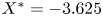 $X^{*}=-3.625$ of the Ahmed body without the presence of the Ahmed-body model: (a) velocity normalised by the free-stream velocity at
  $Z^{*}=1.74$; (b) turbulence intensity (
 $I_x$). Left and right Ahmed-body side-surface boundary-layer profiles at mid-height upstream of separation (
 $X^{*}= -0.05$,
  $Z^{*}=1.74$) for (c) velocity, (d) turbulence intensity, for the empty and grid-generated turbulence cases.
The displacement thicknesses for each case are listed in table 2. The  $\textrm{G}40\_2$ and
  $\textrm{G}40\_6$ boundary layers exhibit a velocity overshoot at
  $Z^{*} = 0.69$ and
  $Z^{*} = 0.25$, respectively; to avoid biasing, the displacement thicknesses for these two cases have been calculated using the velocity at those heights. Figure 2 indicates that the upstream turbulence generation devices thicken the boundary layer to differing extents. A height of
  $Z^{*} = 0.69$ (200 mm) has been used as the reference for
  $U_{\infty }$, the closest measurement to the mid-height of the model, as a somewhat crude representation of the equivalent uniform velocity seen by the body, noting the differences in profiles and boundary-layer height. This is used for normalisation of all data, except for the displacement thickness calculations. Additionally, the mid-height of the model, which is also the height of free turbulence quantification, locates within the boundary layer for all slat cases. We note that this is not dissimilar in condition to a vehicle following in the wake of another. The lateral ground boundary layers (not shown) taken at
  $Y^{*} = \pm 0.69$ were compared to their respective centreline (
 $Y^{*} =0$) boundary layers and showed good agreement; the largest deviation observed at
  $Z^{*} = 0.69$ was 2.5 % for
  $\textrm{G}100\_3$.
2.3.3. Ahmed-body side-boundary-layer profiles
The boundary-layer measurements taken on the side of the model for the grid and empty configurations are presented in figure 2(a). These measurements provide an assessment of the symmetry of the flow and reveal only small deviations between the left and right side boundary layers for specific grid cases. For each grid, the average deviation is less than 1 %. The side boundary layers of different grids follow a similar trend, noting that there are slight overshoots in the ground boundary layer for the  $\textrm{G}40\_2$ and
  $\textrm{G}40\_6$ cases, which likely explains the offset of these to the other measurements. The turbulence intensity values shown for each grid in figure 2(b) reach a consistent value at lateral points outside of the side boundary layer.
2.3.4. Turbulence length scale based on von Kármán spectra
The von Kármán spectra, expressed in (2.3a,b) below, allowed for a determination of turbulence length scales ( $L_x$,
  $L_y$,
  $L_z$) when fit to the normalised power spectra of the velocity measurements. These velocity data were recorded at a location
  $X^{*} = -3.625$, vertically above the splitter plane at the centreline (
 $Y^{*} = 0$), at
  $Z^{*} = 0.69$, close to the mid-height of the model. Each power spectra was obtained using a Hamming window, splitting the signal into 1 s segments with 75 % overlap. A least-squares fitting method was applied to fit the experimental spectrum on a logarithmic plot. The length-scale-dependent fits are provided by von Kármán (Reference von Kármán1948):
 \begin{align} &{\dfrac{fP_{xx}}{\sigma_{u}^{2}}=\dfrac{4L_xf_x}{U_\infty}\dfrac{1}{{\left(1+\dfrac{1.339L_x2{\rm \pi} f_x}{U_\infty}\right)}^{{5}/{6}}}}; \quad {\dfrac{fP_{xx}}{\sigma_{u}^{2}}}=\dfrac{4L_if_i}{U_\infty} \dfrac{1+\dfrac{8}{3}{\left(\dfrac{2.678L_i2{\rm \pi} f_i}{U_\infty}\right)}^{2}} {\left(1+\left(\dfrac{2.678L_i2{\rm \pi} f_i}{U_\infty}\right)^{2}\right)^{{11}/{6}}}\nonumber\\ &\quad i=\left\{ y,z \right\}. \end{align}
 The fitting procedure for the longitudinal velocity component is illustrated in figure 3. In this figure, the Strouhal number ( ${St}$) was normalised by model height (
 $H$), velocity (
 $U_{\infty }$), and the Power Spectral Density (
 $f\cdot P_{xx}$) was normalised by the signal variance (
 $\sigma _{u}^{2}$).

Figure 3. Illustration of turbulence-length-scale calculation in the longitudinal direction based on von Kármán fitting (black axes) for configurations: (a) empty/no turbulence device, (b) 40 mm slats at 4 m, (c) 40 mm grids at 2 m, (d) 100 mm grids at 3 m.
2.4. Bistability quantification
A key challenge was how to identify whether the wake was skewed to one side or the other, or indeed switching. On this point, this phenomenon had been observed as an asymmetric wake and, interestingly, the cause was often attributed to biased upstream flows, model misalignment or model imperfections. In this study, the base-pressure gradient in both the lateral and vertical direction was used to identify long-term stable states. Specifically, the indicative lateral ( ${\partial {C_P}}/{\partial {y}}$) and vertical (
 ${\partial {C_P}}/{\partial {z}}$) pressure gradients were calculated based on the mean pressure difference between left–right and top–bottom sections, respectively. Additionally, a median filter of
  $T^{*} = U_{\infty }t/H = 20$,
  $\sim$0.4 s, was applied to
  ${\partial {C_P}}/{\partial {y}}$ and
  ${\partial {C_P}}/{\partial {z}}$ to filter out higher frequency noise and to make it easier to determine and extract the presence of switching between the two bistable states. After the filter was applied, each zero crossing of the gradients was counted as a switch; this approach was sufficient to separate the switching events from the typical scales of vortex shedding.
3. Results
The bistability characteristics for four representative cases of low to high free-stream turbulence conditions are compared in § 3.1, and a statistical illustration of how the bistability behaves during the transition between the two representative cases is revealed in § 3.2.
3.1. Bistability at low and high background turbulence
With reference to table 2, four turbulence configurations ( $Empty$,
  $\textrm{S}40\_4$,
  $\textrm{G}40\_2$ and
  $\textrm{G}100\_3$) were selected as representative of wake bistability characteristics subject to a range of background turbulence conditions. As indicated,
  ${\partial {C_P}}/{\partial {y}}$ and
  ${\partial {C_P}}/{\partial {z}}$ are utilised to capture the potential lateral and vertical bistability, and the non-dimensional time series. The corresponding probability distributions are illustrated in figure 4(a,d) (lateral) and figure 4(b,e) (vertical). Using the filtered signals, it is possible to distinguish the state-shifting more clearly from the background noise. The two bistable states in the lateral direction are visualised by conditionally averaging the base pressure according to the sign of
  ${\partial {C_P}}/{\partial {y}}$, where we have set
  ${\partial {y} = W/2}$, and the results are illustrated in figure 4(c,f). The white cross markers highlight the locations of minimum pressure for each state.

Figure 4. Comparison of the bistability characteristics between the Empty,  $\textrm{S}40\_4$,
  $\textrm{G}40\_2$ and
  $\textrm{G}100\_3$ cases: (a,d) lateral bistability quantified by
  ${\partial {C_P}}/{\partial {y}}$ signal and corresponding probability distribution; (b,e) vertical bistability quantified by
  ${\partial {C_P}}/{\partial {z}}$ signal and corresponding probability distribution; (c,f) phase-averaged relative pressure coefficient (
 ${\Delta C_P = C_P - \bar {C}_P }$) illustrating the bistability at left and right state. White cross shows location of minimum pressure.
In figure 4(a,d), the base pressure shows distinct lateral bistability at low free-stream turbulence, with clear evidence of two near mirror-symmetrical states at  ${\partial {C_P}}/{\partial {y}} = \pm 0.3$, for all cases. Despite the range of turbulence intensities and flow profiles, figure 4(c,f) shows a high consistency between the conditional-averaged pressure contours for each state, for example, the horizontal position of the pressure minima consistently locate at [
 $Y^{*} = \pm 0.33$].
Interestingly, there appear to be three regimes. First ( $\textrm{RI}$), where random switching is clear in both the filtered and unfiltered signals, observed in the empty case (
 $I_x = 1\,\%$),
  $\textrm{G}40\_6$ (
 $I_x = 4\,\%$) and
  $\textrm{G}40\_2$ (
 $I_x = 9\,\%$). Here the filtered
  ${\partial {C_P}}/{\partial {y}}$ signal switches between states and exhibits low variation, indicating in a given state the pressure barycentres are stable. In comparison, the switching between two states in
  $\textrm{S}40\_3$ (
 $I_x = 6\,\%$) and
  $\textrm{G}100\_3$ (
 $I_x = 15\,\%$) is less easily distinguished from the raw time trace, although it is clearer in the filtered signal and probability distribution. In this second regime (
 $\textrm{RII}$), while favouring a positive or negative state, the filtered
  ${\partial {C_P}}/{\partial {y}}$ begins to meander about the mean of each state, likely associated with less stable recirculation. A possible third regime (
 $\textrm{RIII}$) is present (not shown) seen at only in the two highest turbulence slat cases (
 $\textrm{S}100\_4$ and
  $\textrm{S}200\_4$), where the magnitude of the
  ${\partial {C_P}}/{\partial {y}}$ fluctuations are so high that a bimodality in the probability distributions is not obviously apparent, see figure 5(c,d). This may also be interpreted as an extension of regime
  $\textrm{RII}$ under increased meandering. The existence of bistability at low and high turbulence cases suggests that the presence of bistability is an inherent feature regardless of background turbulence. Specifically, the two bistable states still exist at a higher turbulence level, but the higher switching rate (and increased meandering) makes them more difficult to distinguish from the pressure gradient signal alone. In comparison, no bistability is seen in the vertical direction, as the probability density distributions of
  ${\partial {C_P}}/{\partial {z}}$ show only single peaks, as illustrated in figure 4(b,e).

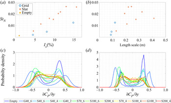
Figure 5. Correlation between bistability switching frequency ( $St$) and (a) turbulence intensity, (b) turbulence length scale, and probability density profiles of lateral pressure gradient without (c) and with (d) filter.
3.2. Effects of turbulence level
The frequency of switching between two bistable states is an important characteristic of bistability, and in this study it is quantified by the average non-dimensional switching rate within the 10 min sampling time (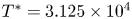 $T^{*} = 3.125 \times 10^{4}$), denoted by
  $St_{N} = N / T^{*}$, where the number of switches (
 $N$) is based on the sign-change of the filtered transverse pressure gradient (
 ${\partial {C_P}}/{\partial {y}}$) and is the average of all tests for each configuration.
For the empty and the grid cases, the switching rates and standard deviation ( $\sigma _{N}$) of the switching rate expressed as
  $St_{N} \pm \sigma _{N}$ were as follows: empty,
 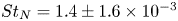 $St_{N} = 1.4 \pm 1.6 \times 10^{-3}$;
  $\textrm{G}40\_6$,
  $St_{N} = 2.1 \pm 2.3 \times 10^{-3}$;
  $\textrm{G}40\_2$,
  $St_{N} = 4.7 \pm 6.3 \times 10^{-3}$;
  $\textrm{G}100\_3$,
  $St_{N} = 1.3 \pm 1.3 \times 10^{-2}$. The switching rate is between one or two orders of magnitude slower than the large-scale oscillations in the near-wake (i.e.
  $St = 0.17$). The ratio
  $\sigma _{N}:St_{N}$ is of the order of 1, and appears to decrease slightly with increased turbulence.
Here  $St_{N}$ increases with turbulence intensity and we observe that the regimes identified in § 3.1 also correspond to ranges of
  $St_{N}$, where
  $St_{N} < 1 \times 10^{-2}$ are
  $\textrm{RI}$,
  $1 \times 10^{-2} < St_{N} < 2.4 \times 10^{-2}$ are
  $\textrm{RII}$, and
  $St_{N} > 2.4 \times 10^{-2}$ are
  $\textrm{RIII}$. There is some sensitivity of
  $St_{N}$ to the filter duration; increasing the time of the median filter necessarily results in a decrease in
  $N$; however, we have selected the filter as a balance between capturing low time-duration symmetry changes and avoiding counting turbulent fluctuations as switching events. This is a particular challenge in a turbulent environment that perhaps requires separate consideration. Importantly, for a median filter of
  $T^{*} = 100$, we continue to see an increase in
  $St_{N}$ as
  $I_x$ increases, although at a reduced gradient.
In comparison with other studies, these rates are close to those of Grandemange et al. (Reference Grandemange, Gohlke and Cadot2013a), who found a rate of  $St_{N} = 6.7 \times 10^{-4}$, whereas they are lower than in Cadot et al. (Reference Cadot, Almarzooqi, Legeai, Parezanović and Pastur2020) who found a rate of
  $St_{N} = 7.2 \times 10^{-3}$ and
  $St_{N} = 5.7 \times 10^{-3}$, for low and high (6 %) turbulence, respectively. The differences in the sensitivity to turbulence in our results to those of Cadot et al. (Reference Cadot, Almarzooqi, Legeai, Parezanović and Pastur2020) may be caused by a number of factors, which require future attention, including the baseline (low-turbulence) switching rate in each study, the turbulence range (we note that the change in switching rate is least obvious over low-turbulence ranges), Reynolds number (as turbulence may interfere with upstream flow structures, e.g. separated flow at the nose), the approach to identification of a switching event, and other set-up differences.
According to figure 5(a), a possible linear or quadratic relationship exists between  $St_{N}$ and
  $I_{x}$, although different gradients are seen for the grid and the slat cases. Especially for the grid cases where the turbulence is more homogeneous, we find that for the low-turbulence range (
 $I_x \lesssim 5$%) in regime RI, only a small change in switching rate is detected, with a potential explanation being that the turbulent fluctuations are not really sufficient to dominate/override the natural randomness of the near-wake which causes the intrinsic bistability. It could be conjectured that a linear relationship is only applicable over a certain range of turbulence level and that there are other factors at play.
There is no clear reason why the gradients of the slats and grids are different in figure 5(a), the implication is that the relationship between turbulence and switching rate is complex. We do note that the length scales of the grids are  ${\sim }0.35H$, whereas for the slats they are considerably higher
  ${\sim } 0.35$–
 $1.4H$. In addition, the turbulence generated from the slats is likely to have a higher level of non-uniformity. While figure 5(b) shows no relationship between the switching rate (
 $St_{N}$) and the measured turbulence length scales, there is a positive correlation, and effective monotonicity for each of the two turbulence generation mechanisms. Furthermore, the grid method of turbulence generation does produce much more homogeneous turbulence at the Ahmed body, as indicated by relatively flat turbulence (boundary-layer) profiles, shown in figure 2(b,d). In addition, for grid-generated turbulence, the ratio of length scales characterised by streamwise to cross-stream fluctuations (
 $L_x/L_y, L_x/L_z$) was typically found to approach
  ${\sim } 0.4$ at the model position, close to the
  $1:2$ ratio expected for homogeneous turbulence. This is significantly better than instances of this ratio for some of the slat-generated turbulence cases of up to
  $1:6$. While other researchers (Kang et al. Reference Kang, Essel, Roussinova and Balachandar2021) have found an influence of the approaching boundary-layer shape on the bistability, we were not able to correlate characteristics of the boundary layer, e.g. displacement thickness, to the switching rate.
The probability distributions of  ${\partial {C_P}}/{\partial {y}}$ both without and with the filter are provided in figures 5(c) and 5(d), respectively. The colour scheme of blue to red indicates an increasing of background turbulence intensity. Figures 5(e) and 5(f) demonstrate a transition from the two symmetrical bistable peaks gradually merging together to a flat-top single-peaked distribution about the centre point.
4. Discussion
Bistability appears a probabilistic phenomenon, with quasi-stable states that persist for periods significantly exceeding other wake time scales. In low turbulence, the vortical structure of the large recirculation bubble has two stable locations offset from the centreline, resulting in the wake tapering left or right. For the cases tested, there is a direct relationship between the turbulence intensity and the wake-state-shifting frequency. There are three possibilities of the cause of this increase: (i) the turbulence in the free flow alters the distribution of momentum, i.e. on the model's lateral sides, (ii) the turbulence changes the nature of the boundary layers and separating shear layers on either side of the body and (iii) the perturbations in the free stream are sufficient to interrupt the persisting state directly.
We suggest that the phase-shifting is triggered by two interacting submechanisms: a random drift of the pressure centre around the centre of each state (mechanism 1), and base-pressure fluctuation due to wake instability (mechanism 2). When the pressure centre is close to the centreline and the magnitude of base pressure is relatively low, it is more likely to (be able to) cross the centreline and shift to the other bifurcation centre. This is apparent in the temporal path of the pressure centre shown for two turbulence intensity cases, supplementary movie 1 (Empty) and 2 ( $\textrm{G}40\_2$) available at https://doi.org/10.1017/jfm.2021.706, together with centreline
  ${C}_{P}(t)$ and
  ${\partial {C_P}}/{\partial {y} (t)}$.
This hypothesis can explain why the frequency of switching is proportional to the free-stream turbulence. We also note that this seems to accord with the observations of Haffner et al. (Reference Haffner, Borée, Spohn and Castelain2020) who linked the stability of each mode to a mechanism whereby large-scale structures are formed from the forcing and amplification of the shear layer by an interaction between the strong recirculating flow and the opposite shear layer. Given the stability of the mode relies on the strength of the recirculation, it follows that perturbations that disrupt the recirculation will also reduce the stability of the mode. Here we see a link to the unsteadiness in the free-stream flow. The free-stream turbulence increases the base-pressure fluctuation frequency (i.e. mechanism 2) through the separating shear-layer instability, modifying large-scale shedding, while mechanism 1 remains unchanged. Therefore, by increasing the occurrence of large-scale fluctuations to the recirculation bubble, free-stream turbulence increases the chance of satisfying the two conditions simultaneously, thus increasing the frequency of phase-shifting.
It is also particularly noteworthy that, despite the range of incoming flow profiles and turbulence levels, the lateral symmetry breaking modes are still favoured for all cases, and the distribution of the conditionally time-averaged base-pressure profiles are almost unchanged. As a corollary, while the perturbations here are disruptive, they do not prevent the interaction between opposite shear layers, a condition that has been identified during the period of transition between symmetry states with associated increased base pressure, as described by Haffner et al. (Reference Haffner, Borée, Spohn and Castelain2020).
Our hypothesis could be tested by correlating the near-wake velocity field in a plane through the pressure centres (obtainable with high-speed PIV) with the shifting base pressure, and should be investigated in future studies. Given the presence of similar large-time-scale wake dynamics in different aspect ratio rectangular back and axisymmetric wakes, these findings are of wide interest beyond the Ahmed-body geometry.
Finally, a comparison with the recent experimental study of Cadot et al. (Reference Cadot, Almarzooqi, Legeai, Parezanović and Pastur2020) is warranted, where they conclude that turbulence does not enhance the switching rate. Despite their different conclusion, our switching rate data are only weakly contradictory with theirs. In their experiments, they only considered a maximum turbulence level of  ${\sim } 5$%, and for our grid-generated turbulence experiments we find the increase in the switching rate is relatively minor over this range, while they find a very small decrease. It is only at higher turbulence levels that the effect is clearly noticeable. In addition, their experiments were undertaken at a lower Reynolds number where significant flow separation occurs at the front of the body, strongly influencing the side boundary layers upstream of separation. Lastly, the comparison of the slat and grid turbulence findings here suggests that properties of the turbulence are important. For instance, it appears turbulent energy at larger scales has a stronger effect. It seems plausible that if there is more turbulent energy at length scales comparable to the body width then this may more strongly affect switching.
Supplementary movies
Supplementary movies are available at https://doi.org/10.1017/jfm.2021.706.
Declaration of interests
The authors report no conflict of interest.