1 Introduction
The settling of a body through an interface separating two fluids is encountered in a broad variety of situations, both in the geophysical context and in engineering applications. In environmental sciences, aerosols, dust or volcanic ashes settling in the lower atmosphere, as well as marine snow sinking in the upper ocean, face a surrounding fluid medium which may locally comprise large density gradients. The corresponding layers are now recognized as having a strong impact on the settling rate and dispersion characteristics of particles, in the case of both atmospheric inversions (Kellogg Reference Kellogg, Bach, Pankrath and Williams1980; Burns & Chemel Reference Burns and Chemel2015) and oceanic thermoclines and haloclines (Riebesell Reference Riebesell1992; MacIntyre, Alldredge & Gotschalk Reference MacIntyre, Alldredge and Gotschalk1995). This, in turn, makes the underlying hydrodynamical processes relevant to an understanding of several aspects of air pollution, climate variability or oceanic biochemical cycling (Denman & Gargett Reference Denman and Gargett1995; Condie & Bormans Reference Condie and Bormans1997). Fluids involved in internal geophysical processes may also undergo natural discontinuous density and/or viscosity stratifications. These discontinuities are thought to be important in momentum exchanges between several layers of planetary interiors. This is, for instance, the case with the ascent of plumes through the Earth’s mantle or the migration of magma slabs through the crust (Manga, Stone & O’Connell Reference Manga, Stone and O’Connell1993).
Most engineering configurations in which rigid or fluid particles have to cross a horizontal interface involve immiscible fluids. Hence, although effects of density stratification may still be significant, those due to interfacial tension and, possibly, viscosity contrast generally play a leading role in that context, as the three following examples suggest. Removal of non-metallic impurities during steel elaboration is usually achieved by transferring them from metal to slag, frequently with the help of gas bubbles either injected at the bottom of the ladle or produced in situ by a chemical reaction (Poggi, Minto & Davenport Reference Poggi, Minto and Davenport1969; Shannon, White & Sridhar Reference Shannon, White and Sridhar2008). In contacting devices used to achieve liquid–liquid extraction, droplets of a light (respectively heavy) liquid rise (respectively settle) towards an interface through a second heavier (respectively lighter) liquid and eventually coalesce to form a light upper (respectively heavy lower) layer. In encapsulation and in several coating processes, gravity is classically used to drive particles across an interface in order to coat them within the film of light fluid that still surrounds them when they penetrate into the second heavier fluid (Weinstein & Palmer Reference Weinstein, Palmer, Kistler and Schweizer1997). However, applications to drug delivery and cell therapy have recently led to the development of coating strategies for micron-size particles using microfluidic devices. As gravity is barely efficient at such scales, magnetic forcing has been proposed as a surrogate to force paramagnetic microparticles to cross the interface and achieve ultrathin coating (Tsai et al. Reference Tsai, Wexler, Wan and Stone2011).
From the viewpoint of hydrodynamics, the canonical configuration that can provide a basic understanding of the complex phenomena involved in the various applications reviewed above is that of a single rigid sphere moving through a quiescent fluid near and across a deformable, initially flat, interface. So far, most of the available studies in the domain have concentrated on two extreme situations involving immiscible fluids.
The first of them corresponds to the so-called ‘film drainage’ problem, in which the sphere succeeds in crossing the interface only after the liquid film that forms ahead of it as it gets close to the interface has been completely drained. Indeed, film drainage is the slowest step of the breakthrough process under certain conditions. This is so if the particle is small enough or its density is close to that of the two fluids, or if it is released close enough to the interface, which is why this configuration has been considered as a reference to elucidate the hydrodynamic mechanisms governing coalescence under quasi-steady conditions. Film drainage dynamics is also key to determining the capture efficiency in flotation processes, where bubbles are used to remove mineral impurities from a liquid (Stechemesser & Nguyen Reference Stechemesser and Nguyen1999). Pioneering experimental and theoretical investigations of that configuration were carried out by Hartland (Reference Hartland1968, Reference Hartland1969), who established the laws governing the evolution of the film thickness and its longitudinal variations; see also the review by Jeffreys & Davies (Reference Jeffreys, Davies and Hanson1971). A more rigorous theory, clarifying, among other things, the origin of the narrowing of the film in the peripheral region where it connects to the meniscus, was elaborated by Jones & Wilson (Reference Jones and Wilson1978); the influence of gravity on the evolution of the film thickness was then considered by Smith & Van de Ven (Reference Smith and Van de Ven1984).
The ‘opposite’ limit worth mentioning is that of a sphere impacting a free surface normally (most frequently an air–water interface) in the regime where inertia effects dominate over those related to surface tension, and viscosity has a virtually negligible influence. Several aspects of this problem are addressed in the classical treatise by Birkhoff & Zarantonello (Reference Birkhoff and Zarantonello1957), and a recent update was provided by Truscott, Epps & Belden (Reference Truscott, Epps and Belden2014). In this situation, provided that the impact velocity is sufficient, a ‘splash’ characterized by the generation of a circular crown of ligaments and droplets is observed at the free surface. It is accompanied by the development of an air cavity connecting the free surface to the sphere. At some point this cavity snaps, letting the sphere sink with a more or less large cylindrical volume of air attached to its rear half. For moderate-to-low impact velocities, the hydrophilic or hydrophobic nature of the sphere surface has been shown to a have a dramatic effect on the deformation of the free surface (Duez, Ybert & Bocquet Reference Duez, Ybert, Clanet and Bocquet2007; Lee & Kim Reference Lee and Kim2008; Aristoff & Bush Reference Aristoff and Bush2009): the formation of the crown and cavity is only observed with hydrophobic spheres (at the surface of which the fluid–solid contact is of the Cassie–Baxter type, due to air entrapment between roughness elements (De Gennes, Brochard-Wyart & Quéré Reference De Gennes, Brochard-Wyart and Quéré2003)), whereas the impact of smooth hydrophilic spheres gives rise to the generation of an upward jet, resulting in a dome above the initial level of the free surface. On increasing the ratio of inertia to capillary effects, the cavity observed with hydrophobic spheres is found to pinch off either right at the free surface (a configuration referred to as ‘surface seal’ by Aristoff & Bush (Reference Aristoff and Bush2009)), somewhat below the free surface (‘shallow seal’) or closer to the sphere than to the surface (‘deep seal’). The dynamics of the cavity, especially the time and vertical position at which its pinch-off occurs, have been modelled using a potential flow approach based on the cylindrical analogue of the theoretical solution of the so-called Rayleigh–Besant problem governing the collapse of a spherical cavity (Duclaux et al. Reference Duclaux, Caillé, Duez, Ybert, Bocquet and Clanet2007; Aristoff & Bush Reference Aristoff and Bush2009). In the deep-seal configuration, ripples due to the acoustic disturbance generated by the pinch-off have been observed to develop at the cavity surface (Grumstrup, Keller & Belmonte Reference Grumstrup, Keller and Belmonte2007). A similar phenomenon but with a different origin was recently reported by Tan et al. (Reference Tan, Vlaskamp, Denissenko and Thomas2016), who considered the impact of spheres coated with a thin oil film (obtained by using a two-layer configuration where the sphere first crosses an oil layer). In that case, ripples form before the cavity snaps, owing to an instability due to the shear at the oil–water interface.
In contrast to the phenomenology of impacting spheres, the present study is concerned with situations in which no ‘splash’ occurs, due to the moderate density difference between the two fluids and the absence of an initial sphere velocity. In this case, two fundamental configurations have been identified (Maru, Wasan & Kintner Reference Maru, Wasan and Kintner1971; Geller, Lee & Leal Reference Geller, Lee and Leal1986). One corresponds to the ‘film drainage’ situation introduced above. The other is the so-called ‘tailing’ configuration, in which, although the drainage of the film separating the sphere from the interface may not have been completed, the sphere succeeds in crossing the interface by towing a column of the upper fluid into the lower one. This column eventually pinches off, its upper part then receding towards the initial position of the interface while the lower part may remain attached to the sphere. The tailing and impacting configurations clearly exhibit qualitative similarities, the liquid tail being the counterpart of the air cavity. However, viscous effects are generally hardly negligible within the tail, generating significant vorticity levels. Given the comparable densities of the two fluids, this vorticity makes the entire flow field quite different from a potential flow. Hence, the tail dynamics generally dramatically differs from that of a cavity. An example of this may be found in a recent study where a disk initially located at an oil–water interface was pulled down with a constant velocity (Peters et al. Reference Peters, Madonia, Lohse and Van Der Meer2016): the optically determined entrained volume of oil was found to be typically twice as large as Darwin’s drift volume (Darwin Reference Darwin1953) predicted by assuming a potential flow throughout the fluid domain. Surprisingly, few systematic studies have been devoted to the tailing configuration, starting with the investigation of Maru et al. (Reference Maru, Wasan and Kintner1971). These authors were mostly interested in determining the critical conditions under which a sphere cannot reach a static equilibrium at the interface, then sinking in the lower fluid. However, using oil–glycerin and oil–water systems, they also observed various aspects of the tail dynamics, including under certain conditions the development of a Rayleigh–Plateau instability in the late stages. A computational study by Geller et al. (Reference Geller, Lee and Leal1986) extensively considered the tailing configuration under creeping flow conditions. By imposing the sphere velocity (respectively body force), these authors could also monitor the evolution of the drag force (respectively sphere velocity) for contrasting values of the flow characteristic parameters, especially the viscosity ratio. However, due to limitations inherent to the boundary integral method, the computations had to be stopped before the tail pinched off, so that no information was provided regarding the late dynamics of the sphere and tail. More recently, quantitative observations of the interface deformation and induced velocity field generated by the settling of millimetre-size glass spheres in a silicone oil/aqueous solution were reported by Dietrich, Poncin & Li (Reference Dietrich, Poncin and Li2011) using high-speed imaging and particle image velocimetry. In a different context, microscopy techniques were used by De Folter et al. (Reference De Folter, De Villeneuve, Aarts and Lekkerkerker2010) to describe the film drainage and tailing configurations, including various aspects of the late tail dynamics, in the case of micron-size spheres settling through a fluid–fluid interface in a demixed colloid–polymer mixture.
The tailing configuration is also observed in miscible fluid set-ups. Indeed, when a body moves vertically in a linearly stratified environment, the originally horizontal isopycnals are distorted and the body tows a long ‘wake’ made of fluid particles lighter than those located at the same altitude far away from its path. As a result, the drag coefficient characterizing the overall fluid resistance to the body motion may increase dramatically (Torres et al. Reference Torres, Hanazaki, Ochoa, Castillo and Van Woert2000; Yick et al. Reference Yick, Torres, Peacock and Stocker2009). A qualitatively similar phenomenology takes place in the presence of a sharp density stratification. Srdic-Mitrovic, Mohamed & Fernando (Reference Srdic-Mitrovic, Mohamed and Fernando1999) used a two-layer water + alcohol–brine system to determine the settling velocity of spherical particles made of various materials. They concluded that the drag coefficient may increase by an order of magnitude after the sphere has crossed the density interface, yielding much longer residence times close to the interface than predicted on the basis of standard drag laws. Abaid et al. (Reference Abaid, Adalsteinsson, Agyapong and McLaughlin2004) even observed that, due to this increase, the sphere velocity may reverse for some time, so that the particle momentarily ‘levitates’ in a fluid environment lighter than its own density. Detailed experiments were then performed in the low-Reynolds-number regime by Camassa et al. (Reference Camassa, Falcon, Lin, McLaughlin and Parker2009, Reference Camassa, Falcon, Lin, McLaughlin and Mykins2010). These authors also developed a theoretical framework yielding an integral representation of the velocity disturbance induced by the distortion of the isopycnals, from which the drag enhancement may be formally evaluated.
Based on the above state of the art for fluid pairs with comparable densities, the present investigation was carried out with two main goals in mind. The first of these was to investigate the evolution of the interface shape and sphere motion over a broad range of physical conditions, from viscosity-dominated to inertia-controlled situations, and from large to small values of the viscosity ratio between the upper and lower fluid layers. Our second aim was to use the quantitative information provided by experiments and direct numerical simulations to obtain new insight into the physical mechanisms governing specific aspects of this evolution, at both short and long time, and develop quantitative models for some of them. The present paper is the first of a series of two in which we present the most significant results of this investigation. The companion paper (Pierson & Magnaudet Reference Pierson and Magnaudet2017b ), hereafter referred to as PM2, focuses on the dynamics of the sphere and tail in some selected axisymmetric configurations corresponding to contrasting flow conditions. Taking advantage of the combination of experimental and computational results, it also provides a detailed analysis of several mechanisms encountered in the long-term evolution of the receding tail which may be seen as a pre-stretched fluid ligament. Here, in Part 1, we focus on experimental observations of the interface dynamics, starting with a description of the corresponding device, protocol and measurement techniques in § 2. Then, § 3 provides a qualitative description of the ‘zoology’ of interface configurations experimentally observed by varying the physical characteristics of the fluid pairs and those of the sphere. These configurations range from the static situation in which small light spheres are able to float steadily at the interface to those, observed with the largest heaviest spheres, in which the tail breaks up into a myriad of droplets, corresponding to a situation of liquid–liquid fragmentation. In intermediate tailing regimes, the primary pinch-off may take place either close to the sphere or in the vicinity of the interface. We rationalize the ‘zoology’ of interface configurations and pinch-off positions by providing qualitative regime maps. Each of the next three sections is devoted to the analysis and modelling of a specific phenomenon observed within some range of conditions; in each case, the corresponding predictions are compared with observations. Section 4 focuses on conditions under which the sphere can rest at the interface, and provides a flotation criterion based on a static force balance. Section 5 considers the drop which frequently remains attached to the sphere once the tail has pinched off. Using a suitable force balance, scaling laws are derived to predict how the drop volume varies with the fluids and sphere characteristics in two different limits. Finally, § 6 focuses on droplets produced during tail fragmentation. A model based on scaling arguments is set up to predict the average drop radius and identify the physical origin of the breakup in cases where effects of interfacial tension and tail viscosity are both significant. The main findings of the paper are summarized in § 7.
2 Experimental approach
2.1 Experimental device and protocol, measurement and processing techniques
The experiments reported below made use of silicone oil as the upper fluid, while the lower fluid was either distilled water or a mixture of distilled water and glycerin with a
 $79\,\%$
glycerin volume fraction. The device and measurement equipment are sketched in figure 1. Experiments were carried out in a 40 cm high glass tank with a
$79\,\%$
glycerin volume fraction. The device and measurement equipment are sketched in figure 1. Experiments were carried out in a 40 cm high glass tank with a
 $20~\text{cm}\times 20~\text{cm}$
cross-section. Two sides of the tank were made of B270 SuperwiteTM glass to limit optical distortion. To avoid formation of a meniscus along the interface, the upper part of the glass walls was coated with the hydrophobic compound Rain-XTM. Spheres were initially held with an inverted clamp and released gently at the top of a 35 mm long tube; the use of an inverted clamp allows the initial rotation of the spheres to be drastically reduced. To also reduce their lateral drift to a minimum, the tube diameter was selected to be slightly larger than that of the sphere in each case, i.e. different tubes were used according to the sphere diameter. In most cases, the top of the tube stood 9 cm above the interface, thus allowing the spheres to settle in the upper liquid over a 5.5 cm distance; this distance was determined to be sufficient for the spheres to almost reach their terminal velocity before encountering the interface. However, with the least viscous silicone oil, inertia effects may be large and increase the distance required for the spheres to reach their terminal velocity. Therefore another stand was used to support the tube, the top of which was located 12 cm above the interface in that case. All experiments were carried out at room temperature, in the range
$20~\text{cm}\times 20~\text{cm}$
cross-section. Two sides of the tank were made of B270 SuperwiteTM glass to limit optical distortion. To avoid formation of a meniscus along the interface, the upper part of the glass walls was coated with the hydrophobic compound Rain-XTM. Spheres were initially held with an inverted clamp and released gently at the top of a 35 mm long tube; the use of an inverted clamp allows the initial rotation of the spheres to be drastically reduced. To also reduce their lateral drift to a minimum, the tube diameter was selected to be slightly larger than that of the sphere in each case, i.e. different tubes were used according to the sphere diameter. In most cases, the top of the tube stood 9 cm above the interface, thus allowing the spheres to settle in the upper liquid over a 5.5 cm distance; this distance was determined to be sufficient for the spheres to almost reach their terminal velocity before encountering the interface. However, with the least viscous silicone oil, inertia effects may be large and increase the distance required for the spheres to reach their terminal velocity. Therefore another stand was used to support the tube, the top of which was located 12 cm above the interface in that case. All experiments were carried out at room temperature, in the range
 $20\pm 2\,^{\circ }\text{C}$
. Liquids were replaced every day or every two days. Each time they were changed, the tank was washed with a detergent liquid, then rinsed out with tap water approximately 10 times, and dried with a dry duster.
$20\pm 2\,^{\circ }\text{C}$
. Liquids were replaced every day or every two days. Each time they were changed, the tank was washed with a detergent liquid, then rinsed out with tap water approximately 10 times, and dried with a dry duster.
The sphere and interface contours were recorded with a PCO pco.dimax S4 high-speed video camera with a resolution of
 $2016\times 2016$
pixels. The acquisition rate varied from 10 frames per second in the case of very slow sphere motion to 500 frames per second for the fastest settling velocity. To reduce optical distortion caused by the interface, an Opto Engineering TC 4M 120 telecentric lens was used. The detected field of view was approximately
$2016\times 2016$
pixels. The acquisition rate varied from 10 frames per second in the case of very slow sphere motion to 500 frames per second for the fastest settling velocity. To reduce optical distortion caused by the interface, an Opto Engineering TC 4M 120 telecentric lens was used. The detected field of view was approximately
 $15.5~\text{cm}\times 8.1~\text{cm}$
.
$15.5~\text{cm}\times 8.1~\text{cm}$
.
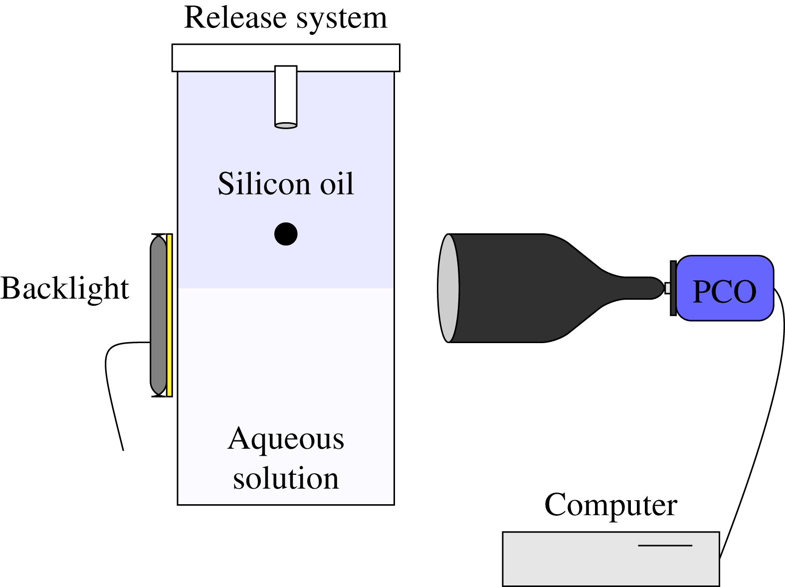
Figure 1. Sketch of the experimental device and optical measurement system.
The contours of the sphere and liquid–liquid interfaces were generally detected using a thresholding method. However, in cases where the lower fluid involved a high percentage of glycerin, the optical contrast between the two fluids was small, making this detection method inaccurate. Therefore, a gradient method was used in such cases. Whatever the detection method, the positions and surfaces detected in each frame were then tracked using a maximum likelihood detection procedure. During the interface breakthrough, optical distortions may affect the detection of the sphere contour. A Hough transform, which allows circles to be recognized on a frame, was then used to extract this contour properly.
Each experiment was repeated at least three times by waiting long enough in between two successive tests for the bath to come back to rest. The results revealed an excellent repeatability, except in the close vicinity of the flotation/sinking transition, where small disturbances, such as dust captured at the sphere surface or variation in the room temperature, could affect the time required for the sphere to detach from the interface significantly. Obviously, in cases exhibiting non-axisymmetric tails, repeatability holds only in a statistical sense, since each realization yields a different instantaneous interface geometry. Nevertheless, these restrictions do not affect the bounds of the various settling regimes to be described in § 3. Repeatability in the axisymmetric regimes can be fully appreciated in PM2, were numerous figures include data provided by the three successive tests. These data are seen to collapse very well in all cases.
2.2 The physical characteristics of the fluids and spheres
The ‘spheres’ were precision marbles manufactured by Marteau et Lemarié, made of stainless steel, aluminium, glass, Teflon (PTFE) and polyacetal (POM) respectively. For each material, we used marbles with nominal diameters of 4, 7, 10 and 14 mm. These diameters were controlled with a
 $\pm 0.02$
mm accuracy with a sliding calliper. The manufacturer’s specifications indicate that their departure from sphericity ranges from
$\pm 0.02$
mm accuracy with a sliding calliper. The manufacturer’s specifications indicate that their departure from sphericity ranges from
 $0.13~\unicode[STIX]{x03BC}\text{m}$
for small steel marbles to
$0.13~\unicode[STIX]{x03BC}\text{m}$
for small steel marbles to
 $25~\unicode[STIX]{x03BC}\text{m}$
for polyacetal marbles, the former having a maximum roughness of
$25~\unicode[STIX]{x03BC}\text{m}$
for polyacetal marbles, the former having a maximum roughness of
 $0.014~\unicode[STIX]{x03BC}\text{m}$
. Their weights were measured with a Mettler Toledo balance with a 1 mg accuracy. The corresponding material densities are given in table 1. They were obtained by averaging over five marbles made of the same material, all with a 7 mm diameter to minimize effects of volume uncertainty. The resulting accuracy of these material densities was
$0.014~\unicode[STIX]{x03BC}\text{m}$
. Their weights were measured with a Mettler Toledo balance with a 1 mg accuracy. The corresponding material densities are given in table 1. They were obtained by averaging over five marbles made of the same material, all with a 7 mm diameter to minimize effects of volume uncertainty. The resulting accuracy of these material densities was
 $\pm 10~\text{kg}~\text{m}^{-3}$
.
$\pm 10~\text{kg}~\text{m}^{-3}$
.
Table 1. Marble densities.
Table 2. The physical properties of the various liquids measured at a temperature of
 $20\,^{\circ }\text{C}$
.
$20\,^{\circ }\text{C}$
.
Table 2 gathers the physical properties of the various fluids or fluid pairs at a reference temperature of
 $20\,^{\circ }\text{C}$
. Liquid densities were measured with a glass gravity hydrometer from Thermo Fisher Scientific with a
$20\,^{\circ }\text{C}$
. Liquid densities were measured with a glass gravity hydrometer from Thermo Fisher Scientific with a
 $\pm 1~\text{kg}~\text{m}^{-3}$
accuracy. Viscosities were determined with a Haake Mars III rheometer (also from Thermo Fisher Scientific). The corresponding relative uncertainty, estimated by determining the viscosity of a given liquid using different ranges of torque, was approximately 3 % for the least viscous oil and was a decreasing function of viscosity. It must be noticed that the viscosity of the water–glycerin mixture is highly temperature-dependent, varying by approximately
$\pm 1~\text{kg}~\text{m}^{-3}$
accuracy. Viscosities were determined with a Haake Mars III rheometer (also from Thermo Fisher Scientific). The corresponding relative uncertainty, estimated by determining the viscosity of a given liquid using different ranges of torque, was approximately 3 % for the least viscous oil and was a decreasing function of viscosity. It must be noticed that the viscosity of the water–glycerin mixture is highly temperature-dependent, varying by approximately
 $25\,\%$
in between
$25\,\%$
in between
 $18\,^{\circ }\text{C}$
and
$18\,^{\circ }\text{C}$
and
 $22\,^{\circ }\text{C}$
. Interfacial tensions were measured with a Kruss DSA 100 tensiometer using the pendant drop technique. The corresponding uncertainty depended on the pair of fluids under consideration. This is because small density differences result in approximately spherical drops, which makes the determination of the interfacial tension more difficult. The uncertainty indicated in table 2 was determined by considering maximum and minimum values obtained over five tests.
$22\,^{\circ }\text{C}$
. Interfacial tensions were measured with a Kruss DSA 100 tensiometer using the pendant drop technique. The corresponding uncertainty depended on the pair of fluids under consideration. This is because small density differences result in approximately spherical drops, which makes the determination of the interfacial tension more difficult. The uncertainty indicated in table 2 was determined by considering maximum and minimum values obtained over five tests.
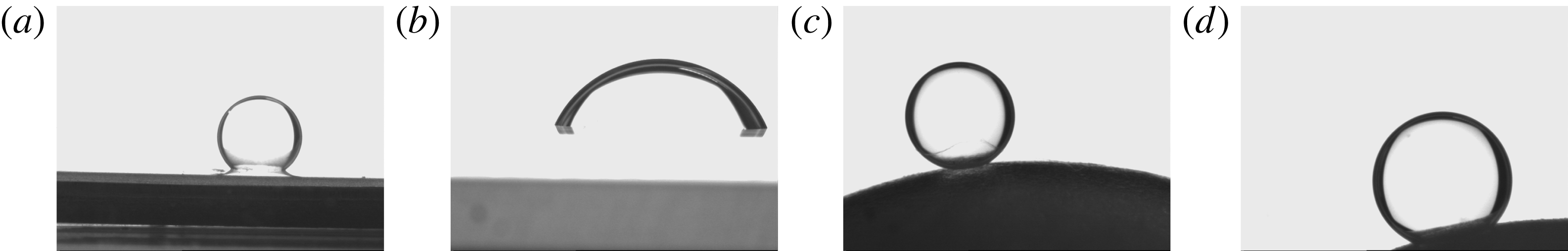
Finally, we determined the macroscopic contact angle at the marble surface in two pairs of fluids, namely V5 oil/water and V5 oil/glycerin+water. We focused on the least viscous silicone oil because it is expected to lead to the fastest film drainage; hence, it is the most favourable to a partial dewetting of the marble surface (De Gennes et al. Reference De Gennes, Brochard-Wyart and Quéré2003). To measure the contact angle, a strip of the material of which the marble was made, or in some cases the marble itself, was introduced into a bath of silicone oil. A drop of water was then released on the solid surface and the contact angle was determined using a Kruss DSA100 tensiometer. The corresponding values (averaged over three tests) are gathered in table 3, and some views of the corresponding three-phase systems are provided in figure 2. These pictures indicate that the solid surface was completely wetted by silicone oil, except in the case of glass, for which partial wetting by water was observed. However, in the course of the dynamic experiments reported below, we never observed the formation of a contact line, even with glass marbles. This is why in the theoretical models described below (and in the computational approach to be described in PM2), we always consider that the sphere is entirely surrounded by a film of silicone oil, i.e. it is never in contact with the lower fluid.

Figure 2. Contact between a drop of water and a solid surface immersed in a bath of V5 silicone oil. (a–d) Steel, glass, Teflon and polyacetal.
Table 3. The contact angle in V5 silicone oil. The superscripts
 $s$
and
$s$
and
 $m$
indicate that measurements were performed on a strip of material or directly on the marble respectively.
$m$
indicate that measurements were performed on a strip of material or directly on the marble respectively.
3 Overall observations and regime maps
3.1 Dimensionless numbers and presentation of observations
Before we start to describe the experimental observations, a prerequisite is the definition of a proper set of dimensionless numbers characterizing the three-phase system. In what follows, index 1 (respectively 2) refers to the upper (respectively lower) fluid, while index
 $p$
refers to the sphere. Assuming that the tank is large enough for confinement effects to be negligible, this system is entirely defined by eight quantities, namely the three densities
$p$
refers to the sphere. Assuming that the tank is large enough for confinement effects to be negligible, this system is entirely defined by eight quantities, namely the three densities
 $\unicode[STIX]{x1D70C}_{1},\unicode[STIX]{x1D70C}_{2},\unicode[STIX]{x1D70C}_{p}$
, the two viscosities
$\unicode[STIX]{x1D70C}_{1},\unicode[STIX]{x1D70C}_{2},\unicode[STIX]{x1D70C}_{p}$
, the two viscosities
 $\unicode[STIX]{x1D707}_{1},\unicode[STIX]{x1D707}_{2}$
, the interfacial tension
$\unicode[STIX]{x1D707}_{1},\unicode[STIX]{x1D707}_{2}$
, the interfacial tension
 $\unicode[STIX]{x1D6FE}$
, the sphere radius
$\unicode[STIX]{x1D6FE}$
, the sphere radius
 $R$
and gravity
$R$
and gravity
 $g$
. Hence, five independent dimensionless numbers may be formed. We select the viscosity ratio
$g$
. Hence, five independent dimensionless numbers may be formed. We select the viscosity ratio
 $\unicode[STIX]{x1D706}=\unicode[STIX]{x1D707}_{2}/\unicode[STIX]{x1D707}_{1}$
, the fluid and solid-to-fluid density contrasts with respect to the upper fluid
$\unicode[STIX]{x1D706}=\unicode[STIX]{x1D707}_{2}/\unicode[STIX]{x1D707}_{1}$
, the fluid and solid-to-fluid density contrasts with respect to the upper fluid
 $\unicode[STIX]{x1D701}=\unicode[STIX]{x1D70C}_{2}/\unicode[STIX]{x1D70C}_{1}-1$
and
$\unicode[STIX]{x1D701}=\unicode[STIX]{x1D70C}_{2}/\unicode[STIX]{x1D70C}_{1}-1$
and
 $\unicode[STIX]{x1D701}_{p}=\unicode[STIX]{x1D70C}_{p}/\unicode[STIX]{x1D70C}_{1}-1$
respectively, the interfacial Bond number
$\unicode[STIX]{x1D701}_{p}=\unicode[STIX]{x1D70C}_{p}/\unicode[STIX]{x1D70C}_{1}-1$
respectively, the interfacial Bond number
 $Bo=g(\unicode[STIX]{x1D70C}_{2}-\unicode[STIX]{x1D70C}_{1})R^{2}/\unicode[STIX]{x1D6FE}$
and the Archimedes number
$Bo=g(\unicode[STIX]{x1D70C}_{2}-\unicode[STIX]{x1D70C}_{1})R^{2}/\unicode[STIX]{x1D6FE}$
and the Archimedes number
 $Ar=\unicode[STIX]{x1D70C}_{1}(\unicode[STIX]{x1D701}_{p}g)^{1/2}R^{3/2}/\unicode[STIX]{x1D707}_{1}$
, which is merely a Reynolds number based on the gravitational velocity
$Ar=\unicode[STIX]{x1D70C}_{1}(\unicode[STIX]{x1D701}_{p}g)^{1/2}R^{3/2}/\unicode[STIX]{x1D707}_{1}$
, which is merely a Reynolds number based on the gravitational velocity
 $(\unicode[STIX]{x1D701}_{p}gR)^{1/2}$
. With the set of fluids described in § 2.2,
$(\unicode[STIX]{x1D701}_{p}gR)^{1/2}$
. With the set of fluids described in § 2.2,
 $\unicode[STIX]{x1D706}$
may be varied by nearly four orders of magnitude, from
$\unicode[STIX]{x1D706}$
may be varied by nearly four orders of magnitude, from
 $\unicode[STIX]{x1D706}=1.9\times 10^{-3}$
with the combination V500/water to
$\unicode[STIX]{x1D706}=1.9\times 10^{-3}$
with the combination V500/water to
 $\unicode[STIX]{x1D706}=18.3$
with V5/glycerin + water. With the same two pairs of fluids,
$\unicode[STIX]{x1D706}=18.3$
with V5/glycerin + water. With the same two pairs of fluids,
 $\unicode[STIX]{x1D701}$
varies by only one order of magnitude, from
$\unicode[STIX]{x1D701}$
varies by only one order of magnitude, from
 $\unicode[STIX]{x1D701}\approx 0.03$
to
$\unicode[STIX]{x1D701}\approx 0.03$
to
 $\unicode[STIX]{x1D701}\approx 0.32$
. The sphere-to-fluid density contrast ranges from
$\unicode[STIX]{x1D701}\approx 0.32$
. The sphere-to-fluid density contrast ranges from
 $0.40$
for polyacetal spheres in V500 oil to
$0.40$
for polyacetal spheres in V500 oil to
 $7.65$
for steel spheres in V5. The interfacial Bond number varies by two orders of magnitude, from
$7.65$
for steel spheres in V5. The interfacial Bond number varies by two orders of magnitude, from
 $0.038$
for the smallest spheres (
$0.038$
for the smallest spheres (
 $R=2$
mm) with the V500/water pair to
$R=2$
mm) with the V500/water pair to
 $4.5$
for the largest ones (
$4.5$
for the largest ones (
 $R=7$
mm) with the V5/glycerin–water pair. Finally, the Archimedes number varies by more than three orders of magnitude, from
$R=7$
mm) with the V5/glycerin–water pair. Finally, the Archimedes number varies by more than three orders of magnitude, from
 $0.33$
with the smallest polyacetal spheres in the V500 oil to
$0.33$
with the smallest polyacetal spheres in the V500 oil to
 $968$
with the largest steel spheres in V5. However, in the lower fluid, the relevant gravitational velocity and viscosity are
$968$
with the largest steel spheres in V5. However, in the lower fluid, the relevant gravitational velocity and viscosity are
 $((\unicode[STIX]{x1D70C}_{p}/\unicode[STIX]{x1D70C}_{2}-1)gR)^{1/2}$
and
$((\unicode[STIX]{x1D70C}_{p}/\unicode[STIX]{x1D70C}_{2}-1)gR)^{1/2}$
and
 $\unicode[STIX]{x1D707}_{2}$
respectively, so that the relevant Archimedes number, say
$\unicode[STIX]{x1D707}_{2}$
respectively, so that the relevant Archimedes number, say
 $Ar_{l}$
, is
$Ar_{l}$
, is
 $Ar_{l}=(1/\unicode[STIX]{x1D706})\left((\unicode[STIX]{x1D701}_{p}-\unicode[STIX]{x1D701})(1+\unicode[STIX]{x1D701})/\unicode[STIX]{x1D701}_{p}\right)^{1/2}Ar$
. Hence, when the viscosity contrast is large,
$Ar_{l}=(1/\unicode[STIX]{x1D706})\left((\unicode[STIX]{x1D701}_{p}-\unicode[STIX]{x1D701})(1+\unicode[STIX]{x1D701})/\unicode[STIX]{x1D701}_{p}\right)^{1/2}Ar$
. Hence, when the viscosity contrast is large,
 $Ar$
and
$Ar$
and
 $Ar_{l}$
may differ by several orders of magnitude for a given sphere. For instance, in the latter two cases with
$Ar_{l}$
may differ by several orders of magnitude for a given sphere. For instance, in the latter two cases with
 $Ar=0.33$
and
$Ar=0.33$
and
 $Ar=968$
, one respectively obtains
$Ar=968$
, one respectively obtains
 $Ar_{l}=169$
and
$Ar_{l}=169$
and
 $Ar_{l}=4815$
when the lower fluid is water. To analyse some specific phenomena, it may also be appropriate to replace
$Ar_{l}=4815$
when the lower fluid is water. To analyse some specific phenomena, it may also be appropriate to replace
 $Bo$
, which only involves the fluid density contrast, by a Bond number based on the solid-to-fluid density contrast with respect to the lower fluid, i.e.
$Bo$
, which only involves the fluid density contrast, by a Bond number based on the solid-to-fluid density contrast with respect to the lower fluid, i.e.
 $Bo_{l}=g(\unicode[STIX]{x1D70C}_{p}-\unicode[STIX]{x1D70C}_{2})R^{2}/\unicode[STIX]{x1D6FE}=(\unicode[STIX]{x1D701}_{p}/\unicode[STIX]{x1D701}-1)Bo$
.
$Bo_{l}=g(\unicode[STIX]{x1D70C}_{p}-\unicode[STIX]{x1D70C}_{2})R^{2}/\unicode[STIX]{x1D6FE}=(\unicode[STIX]{x1D701}_{p}/\unicode[STIX]{x1D701}-1)Bo$
.

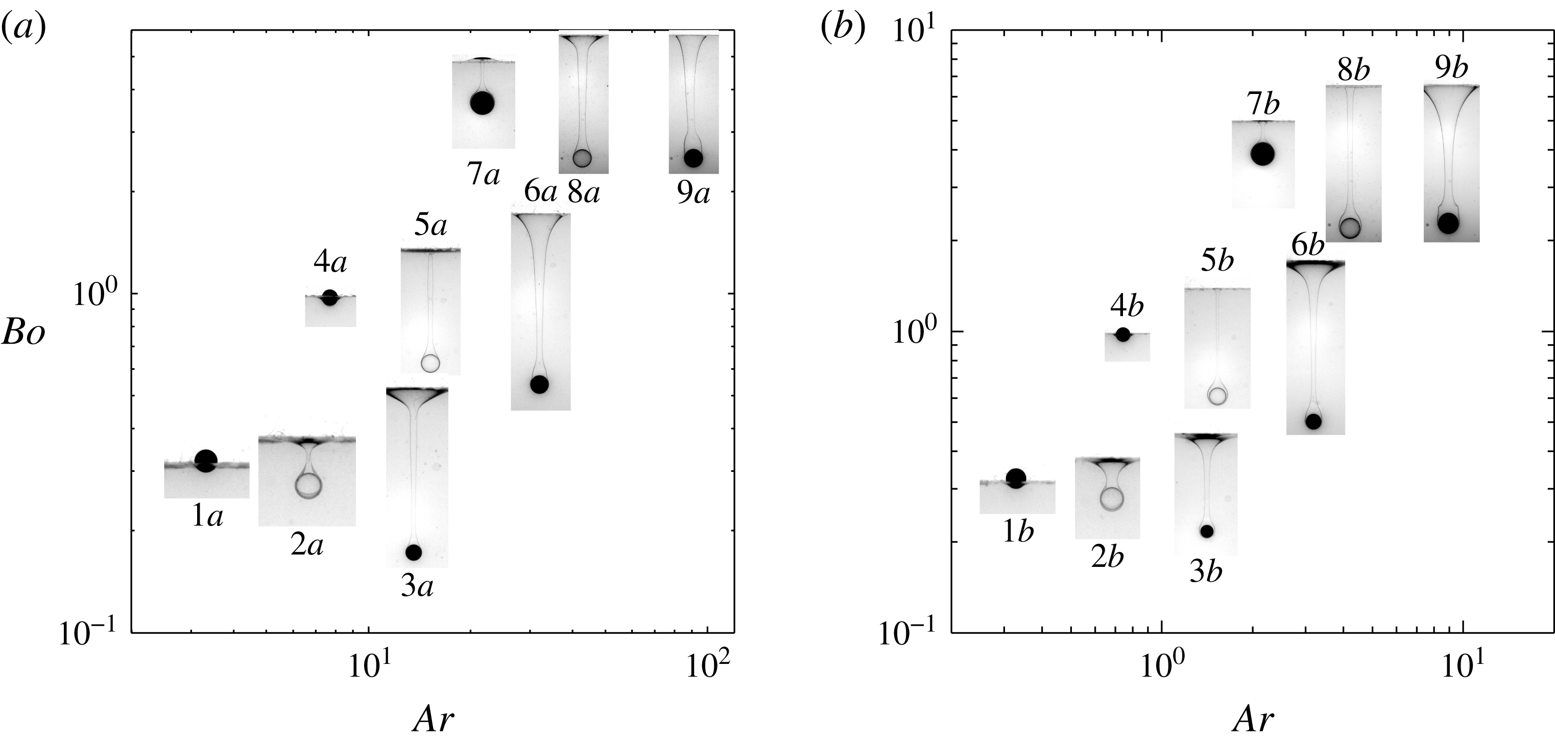
Figure 3. Some selected settling configurations for (a) the V50/water–glycerin pair
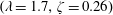 $(\unicode[STIX]{x1D706}=1.7,\unicode[STIX]{x1D701}=0.26)$
and (b) the V500/water–glycerin pair
$(\unicode[STIX]{x1D706}=1.7,\unicode[STIX]{x1D701}=0.26)$
and (b) the V500/water–glycerin pair
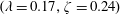 $(\unicode[STIX]{x1D706}=0.17,\unicode[STIX]{x1D701}=0.24)$
. In each panel, from left to right, polyacetal, glass and steel spheres; from top to bottom,
$(\unicode[STIX]{x1D706}=0.17,\unicode[STIX]{x1D701}=0.24)$
. In each panel, from left to right, polyacetal, glass and steel spheres; from top to bottom,
 $R=7,3.5$
and 2 mm. The vertical and horizontal medians of each image are positioned on the appropriate values of
$R=7,3.5$
and 2 mm. The vertical and horizontal medians of each image are positioned on the appropriate values of
 $Ar$
and
$Ar$
and
 $Bo$
respectively.
$Bo$
respectively.

Figure 4. The same as figure 3 for (a) the V5/water–glycerin pair
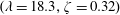 $(\unicode[STIX]{x1D706}=18.3,\unicode[STIX]{x1D701}=0.32)$
and (b) the V5/water pair
$(\unicode[STIX]{x1D706}=18.3,\unicode[STIX]{x1D701}=0.32)$
and (b) the V5/water pair
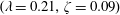 $(\unicode[STIX]{x1D706}=0.21,\unicode[STIX]{x1D701}=0.09)$
.
$(\unicode[STIX]{x1D706}=0.21,\unicode[STIX]{x1D701}=0.09)$
.
To discuss experimental observations in the five-dimensional parameter space
 $(\unicode[STIX]{x1D706},\unicode[STIX]{x1D701},\unicode[STIX]{x1D701}_{p},Bo,Ar)$
, we select a representation in which, for a given pair of fluids, i.e. a given
$(\unicode[STIX]{x1D706},\unicode[STIX]{x1D701},\unicode[STIX]{x1D701}_{p},Bo,Ar)$
, we select a representation in which, for a given pair of fluids, i.e. a given
 $(\unicode[STIX]{x1D706},\unicode[STIX]{x1D701})$
pair, a typical view of the sphere + fluid system corresponding to a given
$(\unicode[STIX]{x1D706},\unicode[STIX]{x1D701})$
pair, a typical view of the sphere + fluid system corresponding to a given
 $\unicode[STIX]{x1D701}_{p}$
is positioned in the
$\unicode[STIX]{x1D701}_{p}$
is positioned in the
 $(Ar,Bo)$
plane. We focus on three materials, namely polyacetal, glass and steel, which, for a given sphere radius, yield ascending values of
$(Ar,Bo)$
plane. We focus on three materials, namely polyacetal, glass and steel, which, for a given sphere radius, yield ascending values of
 $Ar$
. We also select three sphere radii, namely 2, 3.5 and 7 mm, which, for a given material, yield ascending values of both
$Ar$
. We also select three sphere radii, namely 2, 3.5 and 7 mm, which, for a given material, yield ascending values of both
 $Ar$
and
$Ar$
and
 $Bo$
. We found it most convenient to split the results into three series. The first of them corresponds to fluid pairs with
$Bo$
. We found it most convenient to split the results into three series. The first of them corresponds to fluid pairs with
 $\unicode[STIX]{x1D706}>0.1$
and spheres such that
$\unicode[STIX]{x1D706}>0.1$
and spheres such that
 $Ar<10^{2}$
and
$Ar<10^{2}$
and
 $Ar_{l}<10^{2}$
, which yields strictly or approximately axisymmetric configurations (see the discussion in § 3.3). The second series covers the same range of viscosity ratios but focuses on spheres such that
$Ar_{l}<10^{2}$
, which yields strictly or approximately axisymmetric configurations (see the discussion in § 3.3). The second series covers the same range of viscosity ratios but focuses on spheres such that
 $Ar$
is large enough (i.e. typically
$Ar$
is large enough (i.e. typically
 ${>}10^{2}$
) for significant non-axisymmetric effects to take place in the upper fluid and possibly in the lower one. Finally, the third series focuses on fluid pairs with small viscosity ratios
${>}10^{2}$
) for significant non-axisymmetric effects to take place in the upper fluid and possibly in the lower one. Finally, the third series focuses on fluid pairs with small viscosity ratios
 $(\unicode[STIX]{x1D706}\leqslant 0.02)$
and spheres such that the flow is axisymmetric in the upper fluid
$(\unicode[STIX]{x1D706}\leqslant 0.02)$
and spheres such that the flow is axisymmetric in the upper fluid
 $(Ar<10^{2})$
but may turn three-dimensional in the lower one because
$(Ar<10^{2})$
but may turn three-dimensional in the lower one because
 $Ar_{l}\gg Ar$
. The various snapshots showing typical interface deformations in the upcoming figures were taken at different times. Time is of course irrelevant in the case of spheres floating steadily at the interface. In tailing configurations, most pictures were taken before the tail and the sphere separated from each other. However, in figures 4 and 5, we selected some snapshots captured right after the tail pinched off, to emphasize that the primary pinch-off may take place either close to the initial position of the interface or close to the sphere. (Mechanisms yielding these two distinct pinch-off locations will be discussed in § 3.4.) Some snapshots revealing massive fragmentation in the tail are also included in figures 4(b) and 5(a). Obviously, the various snapshots do not provide any insight into the evolution of the sphere dynamics, or in most cases the evolution of the tail dynamics, especially after pinch-off has occurred. These aspects are discussed in detail in PM2 for selected axisymmetric configurations taken from figures 3–5. Nevertheless, it may be pointed out here that, in tailing regimes, pinch-off has little direct influence on the sphere velocity, large decelerations/accelerations only being observed well before it occurs.
$Ar_{l}\gg Ar$
. The various snapshots showing typical interface deformations in the upcoming figures were taken at different times. Time is of course irrelevant in the case of spheres floating steadily at the interface. In tailing configurations, most pictures were taken before the tail and the sphere separated from each other. However, in figures 4 and 5, we selected some snapshots captured right after the tail pinched off, to emphasize that the primary pinch-off may take place either close to the initial position of the interface or close to the sphere. (Mechanisms yielding these two distinct pinch-off locations will be discussed in § 3.4.) Some snapshots revealing massive fragmentation in the tail are also included in figures 4(b) and 5(a). Obviously, the various snapshots do not provide any insight into the evolution of the sphere dynamics, or in most cases the evolution of the tail dynamics, especially after pinch-off has occurred. These aspects are discussed in detail in PM2 for selected axisymmetric configurations taken from figures 3–5. Nevertheless, it may be pointed out here that, in tailing regimes, pinch-off has little direct influence on the sphere velocity, large decelerations/accelerations only being observed well before it occurs.
Figure 5. The same as figure 3 for (a) the V50/water pair (
 $\unicode[STIX]{x1D706}=1.9\times 10^{-2}$
,
$\unicode[STIX]{x1D706}=1.9\times 10^{-2}$
,
 $\unicode[STIX]{x1D701}=0.04$
) and (b) the V500/water pair (
$\unicode[STIX]{x1D701}=0.04$
) and (b) the V500/water pair (
 $\unicode[STIX]{x1D706}=1.9\times 10^{-3}$
,
$\unicode[STIX]{x1D706}=1.9\times 10^{-3}$
,
 $\unicode[STIX]{x1D701}=0.03$
). In (a), images located above the broken line were obtained in the presence of Triton X-100; in the lower (respectively upper) series, the image corresponding to the smallest polyacetal (respectively largest glass) sphere was not saved.
$\unicode[STIX]{x1D701}=0.03$
). In (a), images located above the broken line were obtained in the presence of Triton X-100; in the lower (respectively upper) series, the image corresponding to the smallest polyacetal (respectively largest glass) sphere was not saved.
3.2 General observations
Figure 3 displays the first series of observations corresponding to spheres such that
 $Ar<10^{2}$
and
$Ar<10^{2}$
and
 $Ar_{l}<10^{2}$
in two fluid pairs, corresponding to
$Ar_{l}<10^{2}$
in two fluid pairs, corresponding to
 $\unicode[STIX]{x1D706}=1.7$
and
$\unicode[STIX]{x1D706}=1.7$
and
 $0.17$
respectively (among the various experiments, these viscosity ratios actually vary in the ranges
$0.17$
respectively (among the various experiments, these viscosity ratios actually vary in the ranges
 $1.7\pm 0.2$
and
$1.7\pm 0.2$
and
 $0.17\pm 0.2$
respectively, due to the influence of temperature on the viscosity of the water–glycerin mixture). In both cases, the settling of the smallest two polyacetal spheres yields a configuration in which the sphere floats steadily at the interface (configurations
$0.17\pm 0.2$
respectively, due to the influence of temperature on the viscosity of the water–glycerin mixture). In both cases, the settling of the smallest two polyacetal spheres yields a configuration in which the sphere floats steadily at the interface (configurations
 $1a{-}b$
and
$1a{-}b$
and
 $4a{-}b$
in the figure respectively). In contrast, the largest polyacetal sphere and the smallest glass sphere (configurations
$4a{-}b$
in the figure respectively). In contrast, the largest polyacetal sphere and the smallest glass sphere (configurations
 $7a{-}b$
and
$7a{-}b$
and
 $2a{-}b$
respectively) succeed in crossing the interface in a slow quasi-static manner. In all other cases, although it is slowed down by capillary effects when it reaches the interface, the sphere quickly crosses its initial position and settles through the lower fluid while pulling a long tail of the upper fluid. The corresponding images in figure 3 reveal that the geometry of this tail may vary significantly from one case to another. It is almost cylindrical up to the undisturbed interface position in configurations
$2a{-}b$
respectively) succeed in crossing the interface in a slow quasi-static manner. In all other cases, although it is slowed down by capillary effects when it reaches the interface, the sphere quickly crosses its initial position and settles through the lower fluid while pulling a long tail of the upper fluid. The corresponding images in figure 3 reveal that the geometry of this tail may vary significantly from one case to another. It is almost cylindrical up to the undisturbed interface position in configurations
 $5a{-}b$
in both pairs of fluids as well as for
$5a{-}b$
in both pairs of fluids as well as for
 $8b$
in the V500/water–glycerin pair. Moving towards the right on each row, one observes that, far above the sphere, the tail becomes more conical with a flared base for steel spheres (configurations
$8b$
in the V500/water–glycerin pair. Moving towards the right on each row, one observes that, far above the sphere, the tail becomes more conical with a flared base for steel spheres (configurations
 $3a{-}b$
,
$3a{-}b$
,
 $6a{-}b$
and
$6a{-}b$
and
 $9a{-}b$
), which corresponds to a larger entrainment of the upper fluid. Another feature may be noticed by examining the shape of the tail just at the back of these three spheres. From bottom to top, it is seen that this shape changes from conical to nearly cylindrical, even almost forming an angle with the rest of the tail in the case of configuration
$9a{-}b$
), which corresponds to a larger entrainment of the upper fluid. Another feature may be noticed by examining the shape of the tail just at the back of these three spheres. From bottom to top, it is seen that this shape changes from conical to nearly cylindrical, even almost forming an angle with the rest of the tail in the case of configuration
 $9b$
. These changes are reminiscent of those experienced by the streamlines past a sphere in a homogeneous fluid as the Reynolds number increases, the nearly cylindrical configuration corresponding to a well-developed standing eddy. Comparing figures 3(a) and 3(b), it can be observed that tails pulled by steel spheres are thicker, especially in the top region, in the case of the most viscous oil, i.e. of the smallest
$9b$
. These changes are reminiscent of those experienced by the streamlines past a sphere in a homogeneous fluid as the Reynolds number increases, the nearly cylindrical configuration corresponding to a well-developed standing eddy. Comparing figures 3(a) and 3(b), it can be observed that tails pulled by steel spheres are thicker, especially in the top region, in the case of the most viscous oil, i.e. of the smallest
 $\unicode[STIX]{x1D706}$
. The same remark holds for the thin film around the sphere, which can still be discerned in most cases in (b) but not in (a), indicating that the larger
$\unicode[STIX]{x1D706}$
. The same remark holds for the thin film around the sphere, which can still be discerned in most cases in (b) but not in (a), indicating that the larger
 $\unicode[STIX]{x1D706}$
is the faster the drainage is. Lastly, although no pinch-off has occurred by the time of the frames reported in the two panels, its precursor is present in most cases in the form of a neck slightly above the sphere. In contrast, pinch-off is about to occur at the top of the tail in configuration
$\unicode[STIX]{x1D706}$
is the faster the drainage is. Lastly, although no pinch-off has occurred by the time of the frames reported in the two panels, its precursor is present in most cases in the form of a neck slightly above the sphere. In contrast, pinch-off is about to occur at the top of the tail in configuration
 $5a$
, very close to the initial position of the interface.
$5a$
, very close to the initial position of the interface.
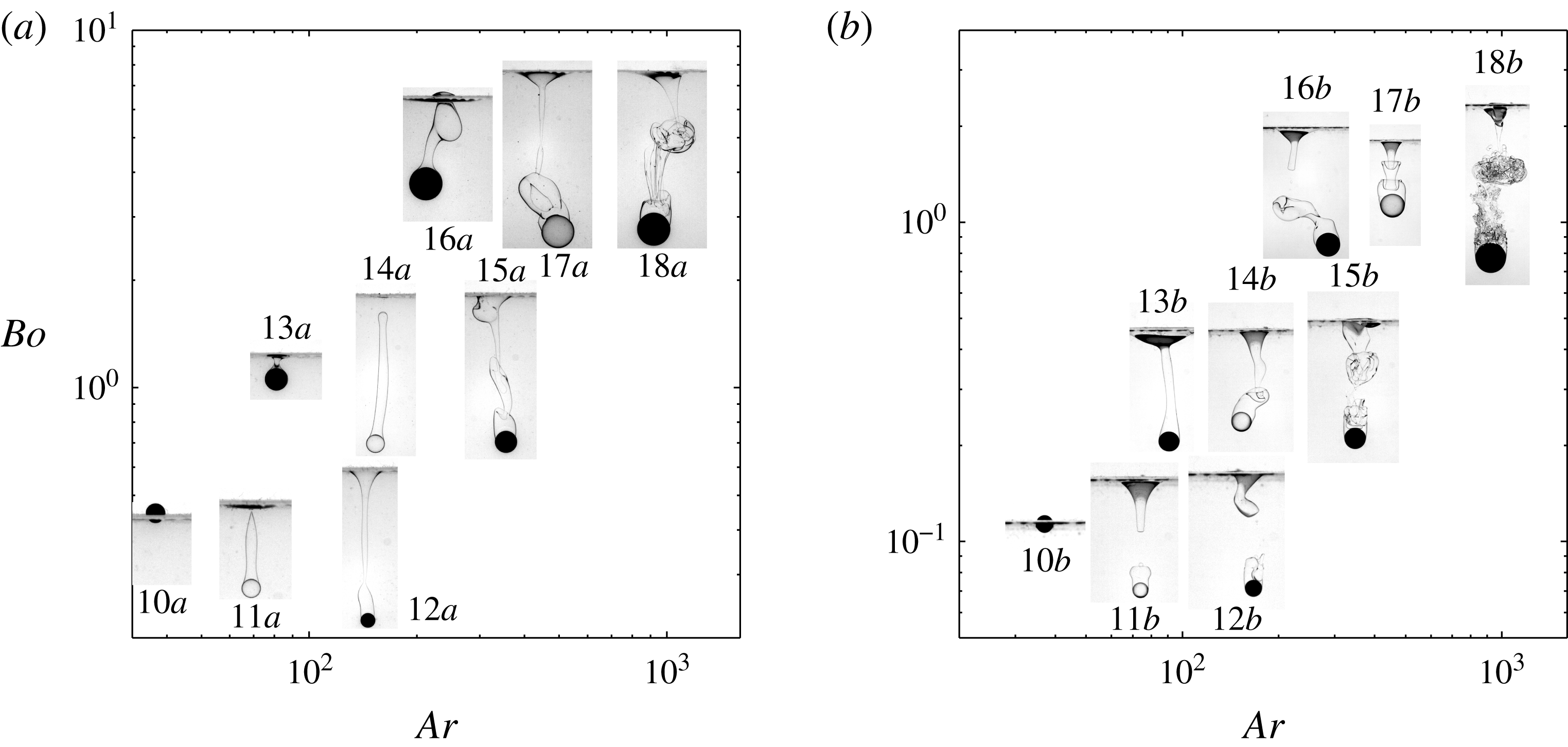
Figure 4 gathers observations corresponding mostly to spheres such that
 $Ar>10^{2}$
in two fluid pairs with
$Ar>10^{2}$
in two fluid pairs with
 $\unicode[STIX]{x1D706}=18.3$
(actually
$\unicode[STIX]{x1D706}=18.3$
(actually
 $18.3\pm 2.2$
depending on the room temperature) and
$18.3\pm 2.2$
depending on the room temperature) and
 $0.21$
respectively. It should be noted that for a given sphere,
$0.21$
respectively. It should be noted that for a given sphere,
 $Ar$
has the same value in (a) and (b) since the upper fluid is the same. Hence, differences observed between them are due to the influence of the lower fluid. This influence is obvious, starting with the smallest glass spheres (configurations 11
$Ar$
has the same value in (a) and (b) since the upper fluid is the same. Hence, differences observed between them are due to the influence of the lower fluid. This influence is obvious, starting with the smallest glass spheres (configurations 11
 $a{-}b$
) and the intermediate polyacetal spheres (configurations 13
$a{-}b$
) and the intermediate polyacetal spheres (configurations 13
 $a{-}b$
). The former two, which correspond to
$a{-}b$
). The former two, which correspond to
 $Ar\approx 70$
, exhibit an axisymmetric tail in both pairs of fluids. However, pinch-off takes place at dramatically different locations. In configuration
$Ar\approx 70$
, exhibit an axisymmetric tail in both pairs of fluids. However, pinch-off takes place at dramatically different locations. In configuration
 $11a$
, the tail breaks right at the initial position of the interface; later on, the sphere settles with a slender column of light fluid attached to its top. In contrast, pinch-off occurs in the lower part of the tail, close to the top of the sphere, in configuration
$11a$
, the tail breaks right at the initial position of the interface; later on, the sphere settles with a slender column of light fluid attached to its top. In contrast, pinch-off occurs in the lower part of the tail, close to the top of the sphere, in configuration
 $11b$
. The latter then goes on settling with a drop of light fluid attached to it, the volume of which is nearly three times its own volume. Similarly, the intermediate polyacetal sphere (configuration
$11b$
. The latter then goes on settling with a drop of light fluid attached to it, the volume of which is nearly three times its own volume. Similarly, the intermediate polyacetal sphere (configuration
 $13a$
) experiences a quasi-static detachment from the interface, whereas a long non-axisymmetric column of light fluid is still developing past the sphere in configuration
$13a$
) experiences a quasi-static detachment from the interface, whereas a long non-axisymmetric column of light fluid is still developing past the sphere in configuration
 $13b$
.
$13b$
.
The three-dimensional nature of the tail is prominent in most other cases, especially when
 $Ar$
and/or
$Ar$
and/or
 $\unicode[STIX]{x1D701}_{p}$
are/is large. In several of them, the topology of the tail strongly resembles that of vortices shed in the wake of a sphere translating in a homogeneous fluid, displaying hairpin-like structures (Sakamoto & Haniu Reference Sakamoto and Haniu1991). For a given sphere with a non-axisymmetric tail, comparison of (a) and (b) makes it clear that three-dimensional effects are significantly stronger in the latter (e.g. configurations 14–16). This is not unlikely since, for a given
$\unicode[STIX]{x1D701}_{p}$
are/is large. In several of them, the topology of the tail strongly resembles that of vortices shed in the wake of a sphere translating in a homogeneous fluid, displaying hairpin-like structures (Sakamoto & Haniu Reference Sakamoto and Haniu1991). For a given sphere with a non-axisymmetric tail, comparison of (a) and (b) makes it clear that three-dimensional effects are significantly stronger in the latter (e.g. configurations 14–16). This is not unlikely since, for a given
 $Ar$
, the actual Archimedes number in the lower fluid,
$Ar$
, the actual Archimedes number in the lower fluid,
 $Ar_{l}$
, is typically 90 times larger in (b), making the Reynolds number
$Ar_{l}$
, is typically 90 times larger in (b), making the Reynolds number
 $Re=\unicode[STIX]{x1D70C}_{2}VR/\unicode[STIX]{x1D707}_{2}$
(
$Re=\unicode[STIX]{x1D70C}_{2}VR/\unicode[STIX]{x1D707}_{2}$
(
 $V$
being the sphere velocity) much larger in the V5/water combination and forcing the corresponding wakes to be in a more advanced transitional stage. In the most inertial case (configuration
$V$
being the sphere velocity) much larger in the V5/water combination and forcing the corresponding wakes to be in a more advanced transitional stage. In the most inertial case (configuration
 $8b$
), fragmentation giving rise to a broad range of droplets and ligaments of light fluid is seen to occur in (b). Premises of fragmentation may also be discerned in configuration
$8b$
), fragmentation giving rise to a broad range of droplets and ligaments of light fluid is seen to occur in (b). Premises of fragmentation may also be discerned in configuration
 $17b$
: thin axisymmetric corollas or ‘inverted skirts’ form at the back of the sphere and propagate downstream, becoming thinner as the distance from the sphere increases.
$17b$
: thin axisymmetric corollas or ‘inverted skirts’ form at the back of the sphere and propagate downstream, becoming thinner as the distance from the sphere increases.
Observations carried out in fluid pairs with very small viscosity ratios
 $(\unicode[STIX]{x1D706}<0.02)$
and with spheres for which
$(\unicode[STIX]{x1D706}<0.02)$
and with spheres for which
 $Ar<10^{2}$
are summarized in figure 5. Under such conditions, the flow is axisymmetric in the upper fluid but may be three-dimensional in the lower one. Some three-dimensionality may be observed in both panels in the most inertial cases, especially in the fragmented region past the most inertial sphere in (a). Actually, this panel displays two distinct series of results. Those located below the broken line were obtained under nominal conditions. In contrast, configurations located above this line (with index
$Ar<10^{2}$
are summarized in figure 5. Under such conditions, the flow is axisymmetric in the upper fluid but may be three-dimensional in the lower one. Some three-dimensionality may be observed in both panels in the most inertial cases, especially in the fragmented region past the most inertial sphere in (a). Actually, this panel displays two distinct series of results. Those located below the broken line were obtained under nominal conditions. In contrast, configurations located above this line (with index
 $s$
standing for ‘surfactant’) were recorded in the presence of Triton X-100 surfactant deliberately added to the distilled water to get some more insight into the influence of the Bond number. We mixed water with a volume of
$s$
standing for ‘surfactant’) were recorded in the presence of Triton X-100 surfactant deliberately added to the distilled water to get some more insight into the influence of the Bond number. We mixed water with a volume of
 $0.6~\text{g}~\text{l}^{-1}$
of Triton X-100 (which is soluble in water but not in silicone oil), corresponding to four times the critical micellar concentration, in order to saturate the interface and prevent the occurrence of any Marangoni effect, even in the presence of strong deformations. While this addition does not modify the viscosity of water, it reduces the interfacial tension by an order of magnitude, yielding
$0.6~\text{g}~\text{l}^{-1}$
of Triton X-100 (which is soluble in water but not in silicone oil), corresponding to four times the critical micellar concentration, in order to saturate the interface and prevent the occurrence of any Marangoni effect, even in the presence of strong deformations. While this addition does not modify the viscosity of water, it reduces the interfacial tension by an order of magnitude, yielding
 $\unicode[STIX]{x1D6FE}=3.3\times 10^{-3}\pm 0.1~\text{Nm}^{-1}$
for the V50/water
$\unicode[STIX]{x1D6FE}=3.3\times 10^{-3}\pm 0.1~\text{Nm}^{-1}$
for the V50/water
 $+$
Triton X-100 fluid pair, instead of
$+$
Triton X-100 fluid pair, instead of
 $30\times 10^{-3}~\text{Nm}^{-1}$
in the nominal case.
$30\times 10^{-3}~\text{Nm}^{-1}$
in the nominal case.
Although the smallest two polyacetal spheres float at the interface of the V50/distilled water pair (configurations
 $19a$
and
$19a$
and
 $22a$
; the image of the former is missing), they are seen to entrain a long tail when the interface is contaminated by Triton X-100 (configurations
$22a$
; the image of the former is missing), they are seen to entrain a long tail when the interface is contaminated by Triton X-100 (configurations
 $19a_{s}$
and
$19a_{s}$
and
 $22a_{s}$
). These two strikingly different behaviours underline the possibility for small light spheres to float or sink, depending on the magnitude of capillary effects. In contrast, the tails developing behind a given steel sphere without or with Triton X-100 (configurations
$22a_{s}$
). These two strikingly different behaviours underline the possibility for small light spheres to float or sink, depending on the magnitude of capillary effects. In contrast, the tails developing behind a given steel sphere without or with Triton X-100 (configurations
 $21a-a_{s}$
,
$21a-a_{s}$
,
 $24a-a_{s}$
and
$24a-a_{s}$
and
 $27a-a_{s}$
respectively) exhibit very similar shapes. This indicates that capillary effects do not play a significant role when the sphere has enough inertia, at least regarding the large-scale geometry of the tail (see the discussion in § 6.2 for their effect on the small-scale structure). Again, thin corollas prefiguring fragmentation and travelling upward along the tail are visible in several cases, especially in configurations
$27a-a_{s}$
respectively) exhibit very similar shapes. This indicates that capillary effects do not play a significant role when the sphere has enough inertia, at least regarding the large-scale geometry of the tail (see the discussion in § 6.2 for their effect on the small-scale structure). Again, thin corollas prefiguring fragmentation and travelling upward along the tail are visible in several cases, especially in configurations
 $26a$
,
$26a$
,
 $23a_{s}$
and
$23a_{s}$
and
 $27b$
. One should note the bulge at the surface of the film that surrounds the sphere in configurations
$27b$
. One should note the bulge at the surface of the film that surrounds the sphere in configurations
 $21b$
,
$21b$
,
 $23b$
,
$23b$
,
 $24b$
and
$24b$
and
 $26b$
. The presence of this bulge suggests that the corollas may have some connection with disturbances born at the surface of the film; the underlying mechanism will be discussed in detail in PM2. A common feature encountered in both pairs of fluids is that tails always neck and later pinch off close to the top of the sphere, giving birth to a drop that remains stuck to it. The volume of this drop may be much larger than that of the sphere itself, as for instance in configuration
$26b$
. The presence of this bulge suggests that the corollas may have some connection with disturbances born at the surface of the film; the underlying mechanism will be discussed in detail in PM2. A common feature encountered in both pairs of fluids is that tails always neck and later pinch off close to the top of the sphere, giving birth to a drop that remains stuck to it. The volume of this drop may be much larger than that of the sphere itself, as for instance in configuration
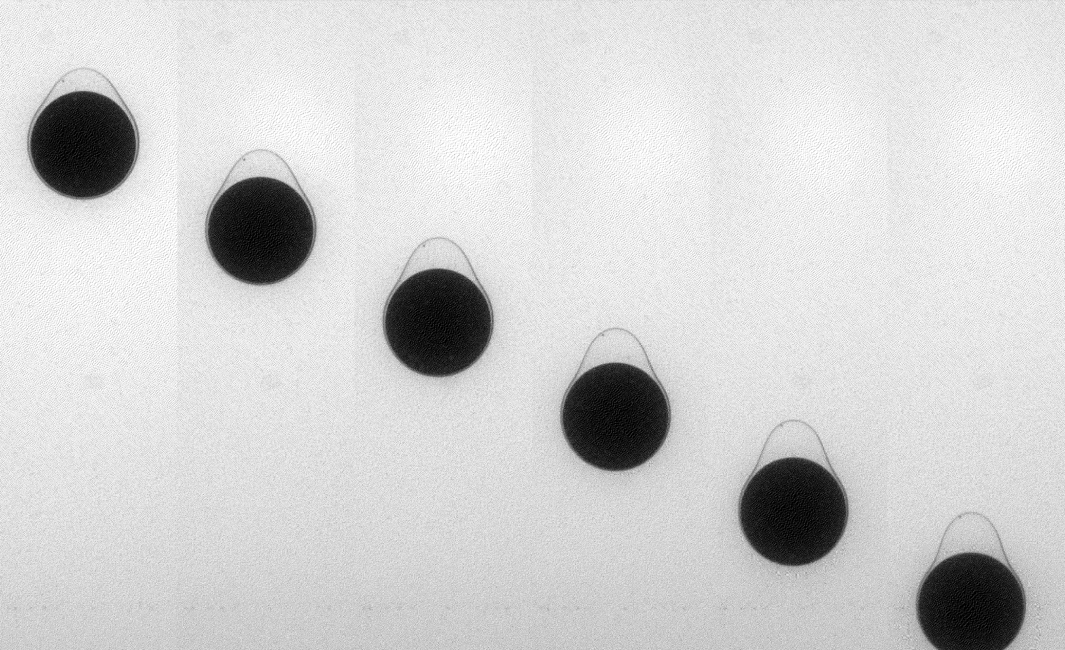
 $20a$
. Finally, consideration of a given sphere successively in (a) and (b) makes it clear that the viscosity of the upper fluid still influences the evolution of the system at the stage displayed in the figure: in some cases, pinch-off has already taken place in (a) whereas it is still to occur in (b); in some others, fragmentation is already present in (a) whereas only its precursor is visible in (b), etc.
$20a$
. Finally, consideration of a given sphere successively in (a) and (b) makes it clear that the viscosity of the upper fluid still influences the evolution of the system at the stage displayed in the figure: in some cases, pinch-off has already taken place in (a) whereas it is still to occur in (b); in some others, fragmentation is already present in (a) whereas only its precursor is visible in (b), etc.
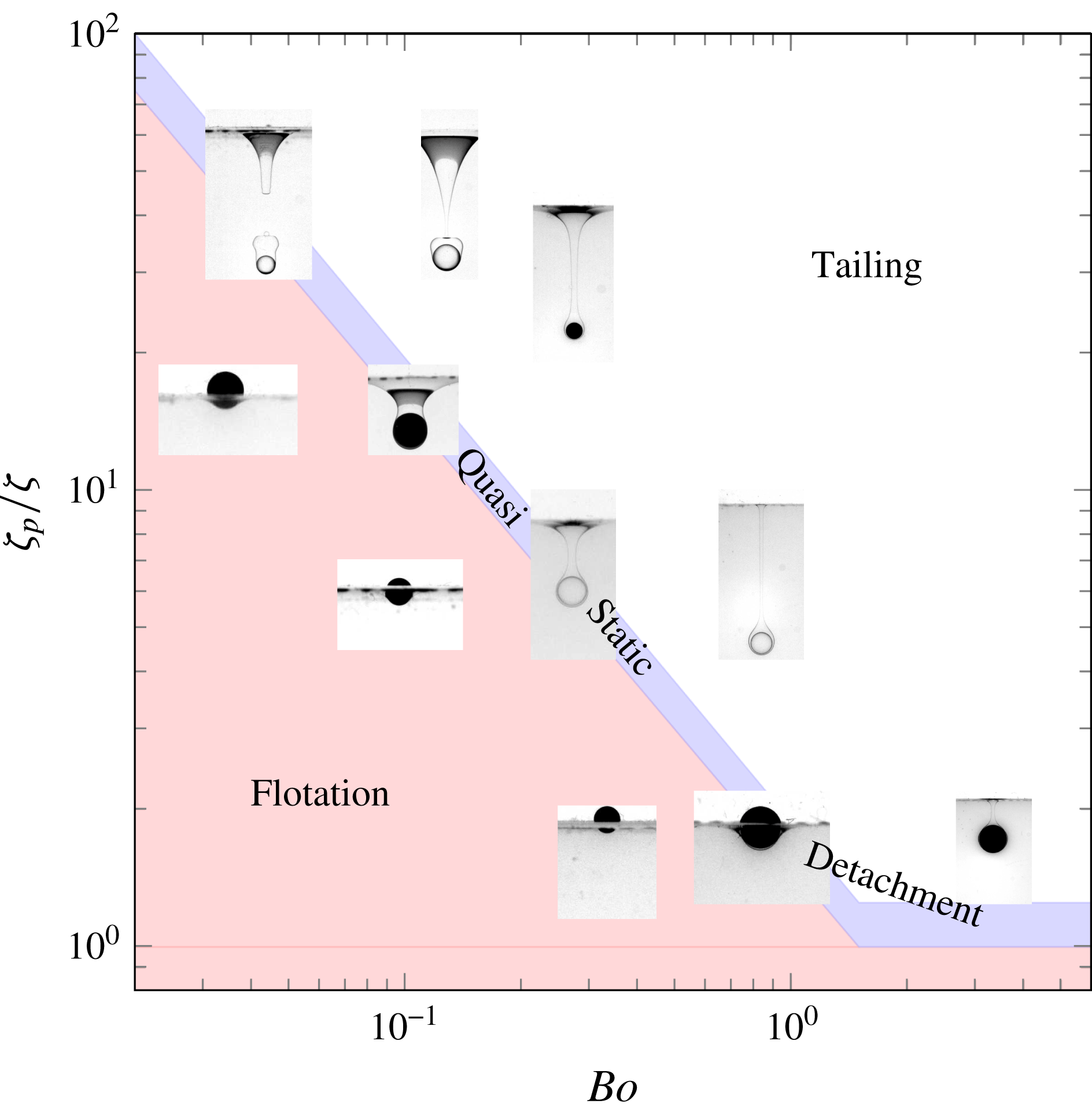
3.3 Regime maps
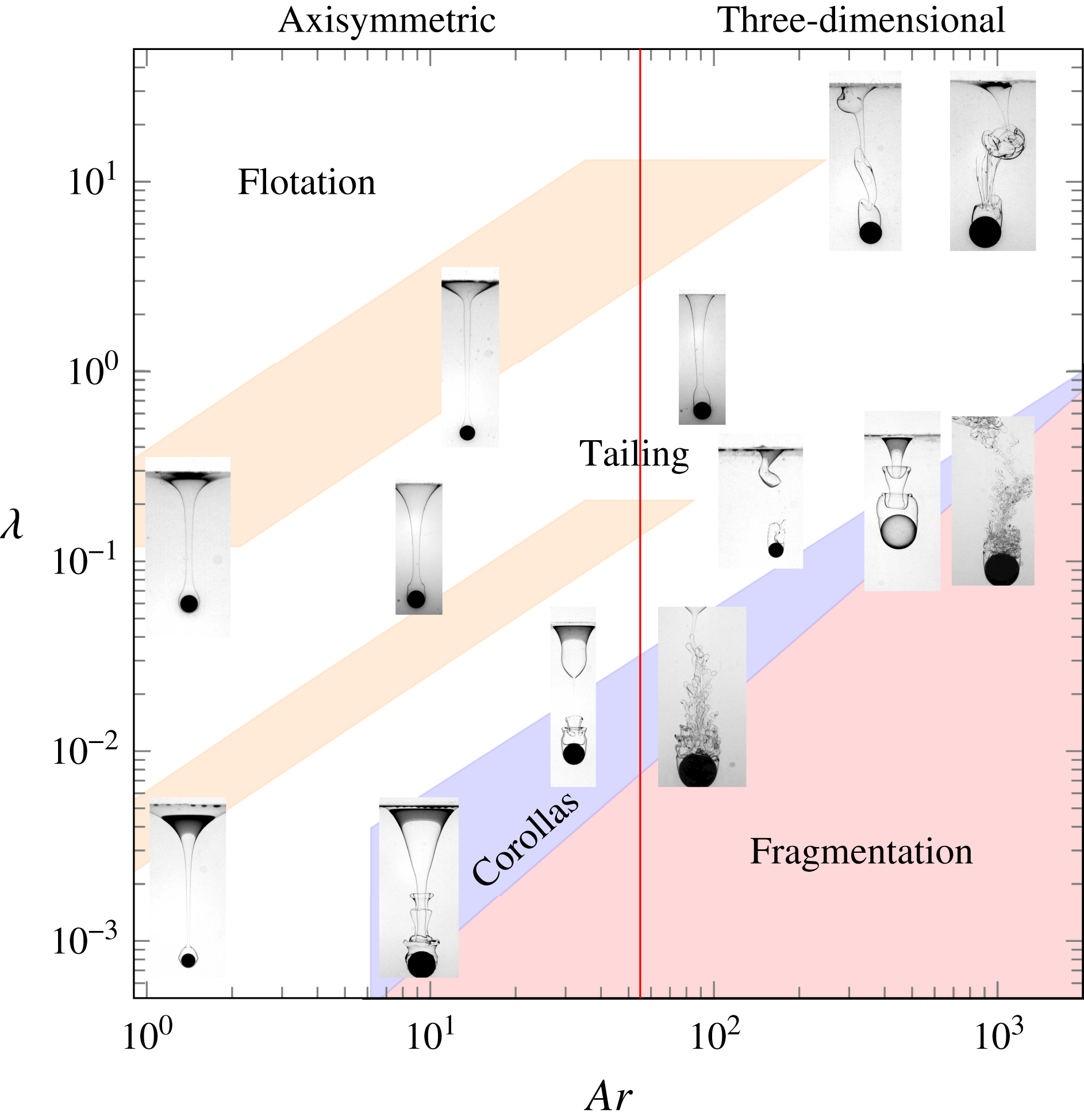
The previous observations reveal a broad variety of phenomena and some classification is desirable. It can be achieved according to the most prominent features seen in the various snapshots of figures 3–5, although such a choice is not unique. According to the mechanisms involved, we consider that the most meaningful classification is one that identifies six distinct regimes, namely flotation at the interface, quasi-steady detachment, axisymmetric and three-dimensional tailing, tailing with peripheral corollas (which may be axisymmetric or three-dimensional) and tail fragmentation. In tailing regimes, subclasses could be introduced according to the position where pinch-off takes place, or, in the post-pinch-off stage, according to the way in which the tail recedes towards the initial position of the interface. We do not consider the latter aspect here, although it will become salient in PM2. It should be noted also that the phenomenon of drops captured by the sphere is common to the quasi-steady detachment and tailing configurations and does not form a specific regime per se.

Figure 6. Regime map showing the distribution of flotation, quasi-static detachment and tailing configurations in the (
 $Bo,\unicode[STIX]{x1D701}_{p}/\unicode[STIX]{x1D701}$
) plane.
$Bo,\unicode[STIX]{x1D701}_{p}/\unicode[STIX]{x1D701}$
) plane.

Figure 7. Regime map showing the distribution of the various tailing configurations, including those with peripheral corollas and tail fragmentation, in the (
 $Ar,\unicode[STIX]{x1D706}$
) plane. The upper (respectively lower) inclined stripe below the flotation region corresponds to the approximate position of the flotation/tailing transition and quasi-steady detachment regimes for set-ups involving the water–glycerin mixture (respectively water alone) as the lower fluid. The vertical line
$Ar,\unicode[STIX]{x1D706}$
) plane. The upper (respectively lower) inclined stripe below the flotation region corresponds to the approximate position of the flotation/tailing transition and quasi-steady detachment regimes for set-ups involving the water–glycerin mixture (respectively water alone) as the lower fluid. The vertical line
 $Ar=55.0$
corresponds to the transition from axisymmetric to three-dimensional flow past the sphere.
$Ar=55.0$
corresponds to the transition from axisymmetric to three-dimensional flow past the sphere.
As stated in § 3.1, the problem under consideration depends on five independent parameters. However, their relative influences are not the same in all regimes, making it possible to draw approximate regime maps by selecting those that are locally most relevant. In figures 3–5, flotation and quasi-static detachment are observed near the bottom-left-hand corner, i.e. with ‘small’ ‘light’ spheres. This is an indication that, under the present conditions, these regimes are primarily governed by static forces, i.e. those due to interfacial tension, gravity and buoyancy, although dynamical effects may become important when the sphere kinetic energy is large enough, as we shall see in § 4.3. Balancing these three static forces and normalizing by the buoyancy force induced by the fluid density contrast introduces
 $Bo$
and
$Bo$
and
 $\unicode[STIX]{x1D701}_{p}/\unicode[STIX]{x1D701}$
as the two key parameters. Figure 6 shows how some selected configurations that were found to correspond to flotation or quasi-static detachment in figures 3–5 gather in the (
$\unicode[STIX]{x1D701}_{p}/\unicode[STIX]{x1D701}$
as the two key parameters. Figure 6 shows how some selected configurations that were found to correspond to flotation or quasi-static detachment in figures 3–5 gather in the (
 $\unicode[STIX]{x1D701}_{p}/\unicode[STIX]{x1D701},Bo$
) diagram, irrespective of the fluid pair under consideration. All floating spheres fall below a critical curve which reveals a sharp decrease of the maximum solid-to-fluid density contrast that allows the sphere to float as the Bond number increases: while capillary effects may sustain spheres much heavier than the lower fluid when
$\unicode[STIX]{x1D701}_{p}/\unicode[STIX]{x1D701},Bo$
) diagram, irrespective of the fluid pair under consideration. All floating spheres fall below a critical curve which reveals a sharp decrease of the maximum solid-to-fluid density contrast that allows the sphere to float as the Bond number increases: while capillary effects may sustain spheres much heavier than the lower fluid when
 $Bo\ll 1$
, buoyancy remains the only mechanism that can counteract the extra weight of the sphere when
$Bo\ll 1$
, buoyancy remains the only mechanism that can counteract the extra weight of the sphere when
 $Bo\gg 1$
(Vella Reference Vella2015). This maximum density contrast is seen to vary by more than an order of magnitude across the range spanned by the Bond number in the present experiments; its variation will be studied in more detail in § 4. Configurations in which spheres are observed to detach from the interface in a quasi-static manner gather within a narrow stripe which follows the above critical curve. The tailing regime takes place beyond this intermediate region.
$Bo\gg 1$
(Vella Reference Vella2015). This maximum density contrast is seen to vary by more than an order of magnitude across the range spanned by the Bond number in the present experiments; its variation will be studied in more detail in § 4. Configurations in which spheres are observed to detach from the interface in a quasi-static manner gather within a narrow stripe which follows the above critical curve. The tailing regime takes place beyond this intermediate region.
Near the top-right-hand corner of figures 3–5, capillary effects do not influence the large-scale features of the observed configurations, although they may still affect the shape of the entrained column locally or the characteristics of structures that form at its periphery (corollas) or within it (ligaments and droplets). The same remark holds for the fluid density contrast, whereas the solid-to-fluid density contrast essentially determines the sphere velocity
 $(V\propto (\unicode[STIX]{x1D701}_{p}gR)^{1/2})$
. Therefore, the corresponding configurations are, to leading order, governed by the balance between inertial and viscous effects in both fluids, i.e. by the parameters
$(V\propto (\unicode[STIX]{x1D701}_{p}gR)^{1/2})$
. Therefore, the corresponding configurations are, to leading order, governed by the balance between inertial and viscous effects in both fluids, i.e. by the parameters
 $Ar$
and
$Ar$
and
 $\unicode[STIX]{x1D706}$
. Based on these remarks, figure 7 displays 13 snapshots extracted from figures 3–5, obtained in the six different pairs of fluids, in the
$\unicode[STIX]{x1D706}$
. Based on these remarks, figure 7 displays 13 snapshots extracted from figures 3–5, obtained in the six different pairs of fluids, in the
 $(Ar,\unicode[STIX]{x1D706})$
plane. Qualitative boundaries are drawn to make the succession of regimes apparent. One of these boundaries, namely the straight line corresponding to
$(Ar,\unicode[STIX]{x1D706})$
plane. Qualitative boundaries are drawn to make the succession of regimes apparent. One of these boundaries, namely the straight line corresponding to
 $Ar=Ar_{c}=55.0$
, is actually exact. It corresponds to the threshold beyond which flow axisymmetry past a freely falling sphere breaks down and the sphere does not follow a strictly vertical path any more, first switching to a slightly oblique path (Fabre, Tchoufag & Magnaudet Reference Fabre, Tchoufag and Magnaudet2012). Intuitively, one could think that the proper criterion to assess flow three-dimensionality in the present case should rather be based on the viscosity of the lower fluid, i.e. on
$Ar=Ar_{c}=55.0$
, is actually exact. It corresponds to the threshold beyond which flow axisymmetry past a freely falling sphere breaks down and the sphere does not follow a strictly vertical path any more, first switching to a slightly oblique path (Fabre, Tchoufag & Magnaudet Reference Fabre, Tchoufag and Magnaudet2012). Intuitively, one could think that the proper criterion to assess flow three-dimensionality in the present case should rather be based on the viscosity of the lower fluid, i.e. on
 $Ar_{l}$
rather than
$Ar_{l}$
rather than
 $Ar$
. However, the wake develops within the tail, i.e. within the upper fluid, making
$Ar$
. However, the wake develops within the tail, i.e. within the upper fluid, making
 $Ar$
the relevant parameter as far as the sphere remains attached to the tail. This argument is fully confirmed in figure 7, where three-dimensional tail geometries are only observed for
$Ar$
the relevant parameter as far as the sphere remains attached to the tail. This argument is fully confirmed in figure 7, where three-dimensional tail geometries are only observed for
 $Ar>Ar_{c}$
, even in cases where
$Ar>Ar_{c}$
, even in cases where
 $Ar_{l}$
is very large (up to
$Ar_{l}$
is very large (up to
 $5\times 10^{3}$
). Not surprisingly, the representation used in figure 7 is of little relevance close to the flotation/tailing transition, which fails to collapse onto a single curve and actually results in two distinct stripes in the left part of the figure. Indeed, for a given fluid pair, i.e. a given
$5\times 10^{3}$
). Not surprisingly, the representation used in figure 7 is of little relevance close to the flotation/tailing transition, which fails to collapse onto a single curve and actually results in two distinct stripes in the left part of the figure. Indeed, for a given fluid pair, i.e. a given
 $\unicode[STIX]{x1D706}$
, the flotation/tailing transition, including the quasi-static detachment regime, spans a non-negligible range of
$\unicode[STIX]{x1D706}$
, the flotation/tailing transition, including the quasi-static detachment regime, spans a non-negligible range of
 $Ar$
, the lower (respectively upper) bound of which corresponds to the smallest (respectively largest) sphere-to-fluid density contrast and Bond number at which this transition is observed in this fluid set-up. Moreover, consider a given sphere settling in two different fluid pairs, say
$Ar$
, the lower (respectively upper) bound of which corresponds to the smallest (respectively largest) sphere-to-fluid density contrast and Bond number at which this transition is observed in this fluid set-up. Moreover, consider a given sphere settling in two different fluid pairs, say
 $A$
and
$A$
and
 $B$
, which differ only by the viscosities of each fluid, i.e.
$B$
, which differ only by the viscosities of each fluid, i.e.
 $\unicode[STIX]{x1D707}_{1}^{A}\neq \unicode[STIX]{x1D707}_{1}^{B}$
and
$\unicode[STIX]{x1D707}_{1}^{A}\neq \unicode[STIX]{x1D707}_{1}^{B}$
and
 $\unicode[STIX]{x1D707}_{2}^{A}\neq \unicode[STIX]{x1D707}_{2}^{B}$
, but have the same
$\unicode[STIX]{x1D707}_{2}^{A}\neq \unicode[STIX]{x1D707}_{2}^{B}$
, but have the same
 $\unicode[STIX]{x1D706}$
, i.e.
$\unicode[STIX]{x1D706}$
, i.e.
 $\unicode[STIX]{x1D706}^{A}=\unicode[STIX]{x1D706}^{B}$
. Then, although
$\unicode[STIX]{x1D706}^{A}=\unicode[STIX]{x1D706}^{B}$
. Then, although
 $Bo$
and
$Bo$
and
 $\unicode[STIX]{x1D701}_{p}/\unicode[STIX]{x1D701}$
are unchanged, the Archimedes numbers associated with the sphere in the two pairs are such that
$\unicode[STIX]{x1D701}_{p}/\unicode[STIX]{x1D701}$
are unchanged, the Archimedes numbers associated with the sphere in the two pairs are such that
 $Ar^{A}/Ar^{B}=\unicode[STIX]{x1D707}_{1}^{B}/\unicode[STIX]{x1D707}_{1}^{A}=\unicode[STIX]{x1D707}_{2}^{B}/\unicode[STIX]{x1D707}_{2}^{A}$
. If
$Ar^{A}/Ar^{B}=\unicode[STIX]{x1D707}_{1}^{B}/\unicode[STIX]{x1D707}_{1}^{A}=\unicode[STIX]{x1D707}_{2}^{B}/\unicode[STIX]{x1D707}_{2}^{A}$
. If
 $Bo$
and
$Bo$
and
 $\unicode[STIX]{x1D701}_{p}/\unicode[STIX]{x1D701}$
have values corresponding to the flotation/tailing transition in figure 6, the two points
$\unicode[STIX]{x1D701}_{p}/\unicode[STIX]{x1D701}$
have values corresponding to the flotation/tailing transition in figure 6, the two points
 $(Ar^{A},\unicode[STIX]{x1D706})$
and
$(Ar^{A},\unicode[STIX]{x1D706})$
and
 $(Ar^{B},\unicode[STIX]{x1D706})$
are distinct in figure 7, and the larger the difference between
$(Ar^{B},\unicode[STIX]{x1D706})$
are distinct in figure 7, and the larger the difference between
 $\unicode[STIX]{x1D707}_{2}^{B}$
and
$\unicode[STIX]{x1D707}_{2}^{B}$
and
 $\unicode[STIX]{x1D707}_{2}^{A}$
is, the larger their separation is. As the water–glycerin mixture has a viscosity that is 88 times that of water, the critical
$\unicode[STIX]{x1D707}_{2}^{A}$
is, the larger their separation is. As the water–glycerin mixture has a viscosity that is 88 times that of water, the critical
 $Ar$
corresponding to this transition for a given
$Ar$
corresponding to this transition for a given
 $\unicode[STIX]{x1D706}$
is much larger in the series involving water alone, which yields the two distinct stripes in figure 7.
$\unicode[STIX]{x1D706}$
is much larger in the series involving water alone, which yields the two distinct stripes in figure 7.
On increasing
 $Ar$
along an iso-
$Ar$
along an iso-
 $\unicode[STIX]{x1D706}$
line, two different successions of regimes are observed, depending on whether
$\unicode[STIX]{x1D706}$
line, two different successions of regimes are observed, depending on whether
 $\unicode[STIX]{x1D706}$
is larger or smaller than a critical value
$\unicode[STIX]{x1D706}$
is larger or smaller than a critical value
 $\unicode[STIX]{x1D706}_{c}\approx 0.1$
. For
$\unicode[STIX]{x1D706}_{c}\approx 0.1$
. For
 $\unicode[STIX]{x1D706}\geqslant \unicode[STIX]{x1D706}_{c}$
, starting from flotation and quasi-static detachment, one successively encounters axisymmetric tails (when the lower fluid is the water–glycerin mixture), then three-dimensional tails, followed by tails with peripheral corollas and eventually tail fragmentation. In contrast, for
$\unicode[STIX]{x1D706}\geqslant \unicode[STIX]{x1D706}_{c}$
, starting from flotation and quasi-static detachment, one successively encounters axisymmetric tails (when the lower fluid is the water–glycerin mixture), then three-dimensional tails, followed by tails with peripheral corollas and eventually tail fragmentation. In contrast, for
 $\unicode[STIX]{x1D706}<\unicode[STIX]{x1D706}_{c}$
(which is achieved only when water is used as the lower fluid), peripheral corollas develop directly on axisymmetric tails and fragmentation takes place for values of
$\unicode[STIX]{x1D706}<\unicode[STIX]{x1D706}_{c}$
(which is achieved only when water is used as the lower fluid), peripheral corollas develop directly on axisymmetric tails and fragmentation takes place for values of
 $Ar$
of the order of
$Ar$
of the order of
 $Ar_{c}$
(as may be noticed in figure 5, the present experiments with
$Ar_{c}$
(as may be noticed in figure 5, the present experiments with
 $\unicode[STIX]{x1D706}=1.9\times 10^{-3}$
were limited to
$\unicode[STIX]{x1D706}=1.9\times 10^{-3}$
were limited to
 $Ar\approx 10$
, so that fragmentation was not observed at such small viscosity ratios, leaving the fragmentation threshold undetermined). For
$Ar\approx 10$
, so that fragmentation was not observed at such small viscosity ratios, leaving the fragmentation threshold undetermined). For
 $Ar\gtrsim 10$
, decreasing
$Ar\gtrsim 10$
, decreasing
 $\unicode[STIX]{x1D706}$
while keeping
$\unicode[STIX]{x1D706}$
while keeping
 $Ar$
constant, one progressively moves from an axisymmetric or three-dimensional tailing regime to tailing with peripheral corollas and eventually tail fragmentation. Keeping in mind that the sphere settles within a fluid at rest at infinity, this succession may be understood by considering the flow region within which velocity gradients are most intense: large (respectively small)
$Ar$
constant, one progressively moves from an axisymmetric or three-dimensional tailing regime to tailing with peripheral corollas and eventually tail fragmentation. Keeping in mind that the sphere settles within a fluid at rest at infinity, this succession may be understood by considering the flow region within which velocity gradients are most intense: large (respectively small)
 $\unicode[STIX]{x1D706}$
corresponds to situations in which shear is large within (around) the tail. Hence, for small
$\unicode[STIX]{x1D706}$
corresponds to situations in which shear is large within (around) the tail. Hence, for small
 $\unicode[STIX]{x1D706}$
, the flow within the tail looks essentially like a plug-type jet peeled off by a strong outer shear, a situation known to be prone to fragmentation (Villermaux Reference Villermaux2007).
$\unicode[STIX]{x1D706}$
, the flow within the tail looks essentially like a plug-type jet peeled off by a strong outer shear, a situation known to be prone to fragmentation (Villermaux Reference Villermaux2007).
3.4 Where does pinch-off take place?
In tailing regimes, the observations reported in figures 3–5 show that the tail may break first very close to the initial position of the interface (e.g. configurations
 $5a$
,
$5a$
,
 $11a$
and
$11a$
and
 $14a$
), close to the sphere (e.g.
$14a$
), close to the sphere (e.g.
 $11b$
,
$11b$
,
 $12b$
and
$12b$
and
 $20a$
) or at some intermediate position (e.g.
$20a$
) or at some intermediate position (e.g.
 $16b$
and
$16b$
and
 $17a$
) in strongly three-dimensional configurations. Among these distinct pinch-off locations, the first two are reminiscent of the ‘shallow seal’/‘deep seal’ classification defined by Aristoff & Bush (Reference Aristoff and Bush2009) in the case of a sphere impacting an air–water surface. To better appreciate how the pinch-off position is influenced by the various control parameters in the present case, we considered all axisymmetric or weakly three-dimensional tailing configurations identified experimentally (including those observed with Teflon and aluminium spheres which do not appear in figures 3–5), plus some results from direct numerical simulations carried out by varying
$17a$
) in strongly three-dimensional configurations. Among these distinct pinch-off locations, the first two are reminiscent of the ‘shallow seal’/‘deep seal’ classification defined by Aristoff & Bush (Reference Aristoff and Bush2009) in the case of a sphere impacting an air–water surface. To better appreciate how the pinch-off position is influenced by the various control parameters in the present case, we considered all axisymmetric or weakly three-dimensional tailing configurations identified experimentally (including those observed with Teflon and aluminium spheres which do not appear in figures 3–5), plus some results from direct numerical simulations carried out by varying
 $Bo,Ar,\unicode[STIX]{x1D706},\unicode[STIX]{x1D701}$
and
$Bo,Ar,\unicode[STIX]{x1D706},\unicode[STIX]{x1D701}$
and
 $\unicode[STIX]{x1D701}_{p}$
independently (the corresponding numerical approach is described in § 2 of PM2). On analysing these results, we noticed that
$\unicode[STIX]{x1D701}_{p}$
independently (the corresponding numerical approach is described in § 2 of PM2). On analysing these results, we noticed that
 $Ar$
has a weak effect on this position, while
$Ar$
has a weak effect on this position, while
 $\unicode[STIX]{x1D701}$
and
$\unicode[STIX]{x1D701}$
and
 $\unicode[STIX]{x1D701}_{p}$
influence it very significantly but essentially through the ratio
$\unicode[STIX]{x1D701}_{p}$
influence it very significantly but essentially through the ratio
 $\unicode[STIX]{x1D701}_{p}/\unicode[STIX]{x1D701}$
, similarly to what happens for the flotation/tailing transition. We also observed significant changes with the Bond number in the range
$\unicode[STIX]{x1D701}_{p}/\unicode[STIX]{x1D701}$
, similarly to what happens for the flotation/tailing transition. We also observed significant changes with the Bond number in the range
 $0.1<Bo<5$
, and a fairly sharp transition with the viscosity contrast for
$0.1<Bo<5$
, and a fairly sharp transition with the viscosity contrast for
 $\unicode[STIX]{x1D706}\approx 0.1$
.
$\unicode[STIX]{x1D706}\approx 0.1$
.
Figure 8. Pinch-off configurations observed in experiments and axisymmetric simulations in fluid set-ups with (a)
 $\unicode[STIX]{x1D706}>0.1$
and (b)
$\unicode[STIX]{x1D706}>0.1$
and (b)
 $\unicode[STIX]{x1D706}\leqslant 0.1$
. In (a), ▿, quasi-static detachment in V5/wg, V50/wg and V500/wg (wg stands for water–glycerin); ▴ (brown) and ▵, shallow and ‘hesitant’ seals in V5/wg respectively; ▪ (brown), ▫ and ▾ (green), shallow, ‘hesitant’ and deep seals in V50/wg respectively;
$\unicode[STIX]{x1D706}\leqslant 0.1$
. In (a), ▿, quasi-static detachment in V5/wg, V50/wg and V500/wg (wg stands for water–glycerin); ▴ (brown) and ▵, shallow and ‘hesitant’ seals in V5/wg respectively; ▪ (brown), ▫ and ▾ (green), shallow, ‘hesitant’ and deep seals in V50/wg respectively;
 $\odot$
and
$\odot$
and
 $\times$
,
$\times$
,
 $+$
and *, shallow, ‘hesitant’ and deep seals with
$+$
and *, shallow, ‘hesitant’ and deep seals with
 $\unicode[STIX]{x1D706}=1$
(numerical). In (b), ▿, quasi-static detachment in V5/w and V50/w; ▫ and ▪, ‘hesitant’ and deep seals in V50/w respectively; ♢ and ♦, ‘hesitant’ and deep seals in V500/w respectively; ▴, deep seal in V50/w+Triton X-100; *, deep seal with
$\unicode[STIX]{x1D706}=1$
(numerical). In (b), ▿, quasi-static detachment in V5/w and V50/w; ▫ and ▪, ‘hesitant’ and deep seals in V50/w respectively; ♢ and ♦, ‘hesitant’ and deep seals in V500/w respectively; ▴, deep seal in V50/w+Triton X-100; *, deep seal with
 $\unicode[STIX]{x1D706}=0.1$
(numerical).
$\unicode[STIX]{x1D706}=0.1$
(numerical).
Based on these observations, figure 8 provides the distribution of the pinch-off style (i.e. ‘shallow’ or ‘deep’) in the
 $(Bo,\unicode[STIX]{x1D701}_{p}/\unicode[STIX]{x1D701})$
plane, separately for
$(Bo,\unicode[STIX]{x1D701}_{p}/\unicode[STIX]{x1D701})$
plane, separately for
 $\unicode[STIX]{x1D706}>0.1$
and
$\unicode[STIX]{x1D706}>0.1$
and
 $\unicode[STIX]{x1D706}\leqslant 0.1$
. In the former case, only axisymmetric or weakly three-dimensional configurations have been considered, since the tail dynamics is enslaved to wake instabilities in fully three-dimensional cases, and pinch-off can then occur at various positions, depending on the details of the shedding process. Some other configurations could not be included because pinch-off took place out of the field of view of the camera, so that its position could not be guaranteed. In addition to shallow and deep types, figure 8 also identifies situations corresponding to quasi-static detachment plus ‘hesitant’ configurations, where pinch-off occurs almost simultaneously at the top and near the bottom of the tail (an example of such situations is discussed in § 4.2 of PM2). According to figure 8(b), only deep-seal-type events are observed beyond the quasi-static detachment regime when
$\unicode[STIX]{x1D706}\leqslant 0.1$
. In the former case, only axisymmetric or weakly three-dimensional configurations have been considered, since the tail dynamics is enslaved to wake instabilities in fully three-dimensional cases, and pinch-off can then occur at various positions, depending on the details of the shedding process. Some other configurations could not be included because pinch-off took place out of the field of view of the camera, so that its position could not be guaranteed. In addition to shallow and deep types, figure 8 also identifies situations corresponding to quasi-static detachment plus ‘hesitant’ configurations, where pinch-off occurs almost simultaneously at the top and near the bottom of the tail (an example of such situations is discussed in § 4.2 of PM2). According to figure 8(b), only deep-seal-type events are observed beyond the quasi-static detachment regime when
 $\unicode[STIX]{x1D706}\leqslant 0.1$
. In contrast, for
$\unicode[STIX]{x1D706}\leqslant 0.1$
. In contrast, for
 $\unicode[STIX]{x1D706}>0.1$
, such events mostly occur either for
$\unicode[STIX]{x1D706}>0.1$
, such events mostly occur either for
 $Bo\gtrsim 3$
or for
$Bo\gtrsim 3$
or for
 $\unicode[STIX]{x1D701}_{p}/\unicode[STIX]{x1D701}\gtrsim 10$
. For
$\unicode[STIX]{x1D701}_{p}/\unicode[STIX]{x1D701}\gtrsim 10$
. For
 $Bo\lesssim 3$
and
$Bo\lesssim 3$
and
 $\unicode[STIX]{x1D701}_{p}/\unicode[STIX]{x1D701}\lesssim 10$
, most pinch-off events take place near the top part of the tail, corresponding to the shallow-seal configuration, but a significant number of ‘hesitant’ configurations also exist. Some complex behaviours may be noticed in figure 8(a), suggesting more subtle influences than just those of
$\unicode[STIX]{x1D701}_{p}/\unicode[STIX]{x1D701}\lesssim 10$
, most pinch-off events take place near the top part of the tail, corresponding to the shallow-seal configuration, but a significant number of ‘hesitant’ configurations also exist. Some complex behaviours may be noticed in figure 8(a), suggesting more subtle influences than just those of
 $Bo$
and
$Bo$
and
 $\unicode[STIX]{x1D701}_{p}/\unicode[STIX]{x1D701}$
. For instance, at
$\unicode[STIX]{x1D701}_{p}/\unicode[STIX]{x1D701}$
. For instance, at
 $Bo\approx 0.3$
, pinch-off is found to be ‘shallow’ for both
$Bo\approx 0.3$
, pinch-off is found to be ‘shallow’ for both
 $\unicode[STIX]{x1D701}_{p}/\unicode[STIX]{x1D701}\approx 12$
and
$\unicode[STIX]{x1D701}_{p}/\unicode[STIX]{x1D701}\approx 12$
and
 $30$
in the V50/water–glycerin set-up, whereas it is ‘deep’ for
$30$
in the V50/water–glycerin set-up, whereas it is ‘deep’ for
 $\unicode[STIX]{x1D701}_{p}/\unicode[STIX]{x1D701}\approx 16$
and 20 in the V5/water set-up.
$\unicode[STIX]{x1D701}_{p}/\unicode[STIX]{x1D701}\approx 16$
and 20 in the V5/water set-up.
To rationalize these observations, scaling arguments are developed in appendix A. As far as the sphere velocity
 $V$
does not change significantly during the breakthrough, i.e. it still scales as
$V$
does not change significantly during the breakthrough, i.e. it still scales as
 $(\unicode[STIX]{x1D701}_{p}gR)^{1/2}$
, the main conclusions are summarized in (A 1). According to these predictions, a ‘shallow’ pinch-off due to capillary effects occurs at a dimensionless time
$(\unicode[STIX]{x1D701}_{p}gR)^{1/2}$
, the main conclusions are summarized in (A 1). According to these predictions, a ‘shallow’ pinch-off due to capillary effects occurs at a dimensionless time
 $\unicode[STIX]{x1D70F}_{\unicode[STIX]{x1D6FE}}^{\ast }$
(normalized by
$\unicode[STIX]{x1D70F}_{\unicode[STIX]{x1D6FE}}^{\ast }$
(normalized by
 $(\unicode[STIX]{x1D701}_{p}g/R)^{1/2}$
) such that
$(\unicode[STIX]{x1D701}_{p}g/R)^{1/2}$
) such that
 $\unicode[STIX]{x1D70F}_{\unicode[STIX]{x1D6FE}}^{\ast }\sim (\unicode[STIX]{x1D701}_{p}/\unicode[STIX]{x1D701})Bo^{1/2}$
. It is readily seen that
$\unicode[STIX]{x1D70F}_{\unicode[STIX]{x1D6FE}}^{\ast }\sim (\unicode[STIX]{x1D701}_{p}/\unicode[STIX]{x1D701})Bo^{1/2}$
. It is readily seen that
 $\unicode[STIX]{x1D70F}_{\unicode[STIX]{x1D6FE}}^{\ast }$
represents the dimensionless length of the tail by the time pinch-off occurs in that configuration; the
$\unicode[STIX]{x1D70F}_{\unicode[STIX]{x1D6FE}}^{\ast }$
represents the dimensionless length of the tail by the time pinch-off occurs in that configuration; the
 $Bo^{1/2}$
scaling is confirmed by the tails seen in figure 4 for configurations
$Bo^{1/2}$
scaling is confirmed by the tails seen in figure 4 for configurations
 $14a$
and
$14a$
and
 $11a$
: the former is
$11a$
: the former is
 $1.8$
longer than the latter, close to the
$1.8$
longer than the latter, close to the
 $1.75$
ratio of the square roots of the corresponding Bond numbers. Conversely, a ‘deep’ pinch-off due to buoyancy effects occurs at a dimensionless time
$1.75$
ratio of the square roots of the corresponding Bond numbers. Conversely, a ‘deep’ pinch-off due to buoyancy effects occurs at a dimensionless time
 $\unicode[STIX]{x1D70F}_{g}^{\ast }\sim (\unicode[STIX]{x1D701}_{p}/\unicode[STIX]{x1D701})^{1/3}$
, and the transition between the two regimes takes place at a critical Bond number
$\unicode[STIX]{x1D70F}_{g}^{\ast }\sim (\unicode[STIX]{x1D701}_{p}/\unicode[STIX]{x1D701})^{1/3}$
, and the transition between the two regimes takes place at a critical Bond number
 $Bo_{t}\sim (\unicode[STIX]{x1D701}_{p}/\unicode[STIX]{x1D701})^{-1/3}$
, only deep (respectively shallow) seal being possible at larger (respectively smaller) Bond numbers. The scaling
$Bo_{t}\sim (\unicode[STIX]{x1D701}_{p}/\unicode[STIX]{x1D701})^{-1/3}$
, only deep (respectively shallow) seal being possible at larger (respectively smaller) Bond numbers. The scaling
 $Bo_{t}\sim (\unicode[STIX]{x1D701}_{p}/\unicode[STIX]{x1D701})^{-1/3}$
suggests a fairly sharp transition between the two styles of pinch-off, as
$Bo_{t}\sim (\unicode[STIX]{x1D701}_{p}/\unicode[STIX]{x1D701})^{-1/3}$
suggests a fairly sharp transition between the two styles of pinch-off, as
 $Bo_{t}$
only varies by a factor of
$Bo_{t}$
only varies by a factor of
 $2$
when
$2$
when
 $\unicode[STIX]{x1D701}_{p}/\unicode[STIX]{x1D701}$
is varied by one order of magnitude. Unfortunately, the data gathered in figure 8 for which the assumption of a nearly constant settling velocity is realistic (i.e. essentially those corresponding to the V50/water–glycerin set-up) do not cover a sufficient range of density contrasts to check this prediction.
$\unicode[STIX]{x1D701}_{p}/\unicode[STIX]{x1D701}$
is varied by one order of magnitude. Unfortunately, the data gathered in figure 8 for which the assumption of a nearly constant settling velocity is realistic (i.e. essentially those corresponding to the V50/water–glycerin set-up) do not cover a sufficient range of density contrasts to check this prediction.
The situation is more complex than expected on the basis of the above scalings in most cases, due to the acceleration or deceleration of the sphere after it has crossed the interface. As shown in appendix A, variations in the sphere velocity result in an additional ‘buoyancy’ effect which shortens (respectively lengthens) the characteristic time
 $\unicode[STIX]{x1D70F}_{g}^{\ast }$
when the sphere accelerates (respectively decelerates), thus decreasing (respectively increasing) the effective critical Bond number
$\unicode[STIX]{x1D70F}_{g}^{\ast }$
when the sphere accelerates (respectively decelerates), thus decreasing (respectively increasing) the effective critical Bond number
 $Bo_{t}$
according to (A 2). The amplitude of the settling velocity variations may be estimated through the ratio of the terminal velocity in the lower fluid to that in the upper one. According to (A 4), this ratio varies approximately as
$Bo_{t}$
according to (A 2). The amplitude of the settling velocity variations may be estimated through the ratio of the terminal velocity in the lower fluid to that in the upper one. According to (A 4), this ratio varies approximately as
 ${\mathcal{C}}(1-\unicode[STIX]{x1D701}/\unicode[STIX]{x1D701}_{p})^{3/5}$
, with
${\mathcal{C}}(1-\unicode[STIX]{x1D701}/\unicode[STIX]{x1D701}_{p})^{3/5}$
, with
 ${\mathcal{C}}=\unicode[STIX]{x1D706}^{-1/5}(1+\unicode[STIX]{x1D701})^{-2/5}$
, provided that
${\mathcal{C}}=\unicode[STIX]{x1D706}^{-1/5}(1+\unicode[STIX]{x1D701})^{-2/5}$
, provided that
 $Ar$
and
$Ar$
and
 $Ar_{l}$
are large enough. In the V50/water (respectively V500/water) pairs of fluids,
$Ar_{l}$
are large enough. In the V50/water (respectively V500/water) pairs of fluids,
 ${\mathcal{C}}$
is approximately
${\mathcal{C}}$
is approximately
 $2.15$
(respectively
$2.15$
(respectively
 $3.4$
). All spheres considered here are such that
$3.4$
). All spheres considered here are such that
 $\unicode[STIX]{x1D701}_{p}/\unicode[STIX]{x1D701}>10$
in these set-ups, so that they all experience significant acceleration effects, which favour deep seal. Figure 8 confirms this trend, as no ‘shallow’ pinch-off is observed in (b), especially in the range
$\unicode[STIX]{x1D701}_{p}/\unicode[STIX]{x1D701}>10$
in these set-ups, so that they all experience significant acceleration effects, which favour deep seal. Figure 8 confirms this trend, as no ‘shallow’ pinch-off is observed in (b), especially in the range
 $Bo<1,10<\unicode[STIX]{x1D701}_{p}/\unicode[STIX]{x1D701}<30$
, where several shallow configurations are identified in (a). In the V5/water–glycerin mixture set-up,
$Bo<1,10<\unicode[STIX]{x1D701}_{p}/\unicode[STIX]{x1D701}<30$
, where several shallow configurations are identified in (a). In the V5/water–glycerin mixture set-up,
 ${\mathcal{C}}\approx 0.50$
, implying a strong deceleration whatever the sphere-to-fluid density contrast. This is why, in that set-up, there exists a range of shallow-seal configurations extending beyond the critical Bond number predicted under the assumption of a constant
${\mathcal{C}}\approx 0.50$
, implying a strong deceleration whatever the sphere-to-fluid density contrast. This is why, in that set-up, there exists a range of shallow-seal configurations extending beyond the critical Bond number predicted under the assumption of a constant
 $V$
. In contrast, the V5/water and V50/water–glycerin set-ups have
$V$
. In contrast, the V5/water and V50/water–glycerin set-ups have
 ${\mathcal{C}}\approx 1.33$
and
${\mathcal{C}}\approx 1.33$
and
 $0.82$
respectively, so that the settling velocity of dense enough spheres is expected to slightly increase in the former and experience little variation in the latter. In figure 8(a), examination of the critical Bond number corresponding to the shallow seal/deep seal transition in the range
$0.82$
respectively, so that the settling velocity of dense enough spheres is expected to slightly increase in the former and experience little variation in the latter. In figure 8(a), examination of the critical Bond number corresponding to the shallow seal/deep seal transition in the range
 $4\lesssim \unicode[STIX]{x1D701}_{p}/\unicode[STIX]{x1D701}\lesssim 6$
fully confirms the influence of acceleration/deceleration effects anticipated on the above basis: while this transition takes place in the range
$4\lesssim \unicode[STIX]{x1D701}_{p}/\unicode[STIX]{x1D701}\lesssim 6$
fully confirms the influence of acceleration/deceleration effects anticipated on the above basis: while this transition takes place in the range
 $1<Bo<2$
in the V50/water–glycerin set-up (
$1<Bo<2$
in the V50/water–glycerin set-up (
 ${\mathcal{C}}\approx 1$
), it occurs in the range
${\mathcal{C}}\approx 1$
), it occurs in the range
 $0.3<Bo<0.6$
in the V5/water system (
$0.3<Bo<0.6$
in the V5/water system (
 ${\mathcal{C}}>1$
) and most probably beyond
${\mathcal{C}}>1$
) and most probably beyond
 $Bo=3$
in the V5/water–glycerin set-up (
$Bo=3$
in the V5/water–glycerin set-up (
 ${\mathcal{C}}<1$
) since a shallow pinch-off is still detected for
${\mathcal{C}}<1$
) since a shallow pinch-off is still detected for
 $Bo=2.2$
. The above findings indicate that, under the present conditions, the viscosity ratio primarily affects the pinch-off dynamics through the sphere acceleration or deceleration, although other viscous effects are possible when
$Bo=2.2$
. The above findings indicate that, under the present conditions, the viscosity ratio primarily affects the pinch-off dynamics through the sphere acceleration or deceleration, although other viscous effects are possible when
 $\unicode[STIX]{x1D706}$
is large, as mentioned in appendix A.
$\unicode[STIX]{x1D706}$
is large, as mentioned in appendix A.
The pinch-off configurations encountered here are reminiscent of those previously described in the context of spheres impacting a free surface (Truscott et al. Reference Truscott, Epps and Belden2014). However, despite obvious similarities, such as the role of capillary and buoyancy forces in the shallow and deep styles of pinch-off respectively, many differences exist. For instance, no splash is observed at the interface in the present experiments, whereas spectacular splash curtains are known to take place when a hydrophobic sphere impacts a free surface with a large enough velocity, a situation yielding a specific ‘surface-seal’ configuration (Aristoff & Bush Reference Aristoff and Bush2009). Connections and fundamental differences between the tail dynamics that develop in liquid–liquid systems and the dynamics of air cavities that form in impact situations are further discussed in appendix B.
4 When can the sphere float?
Observations reviewed in § 3.2, summarized in the phase diagram of figure 6, revealed that small and light enough spheres do not succeed in crossing the interface and keep on floating on it for ever. In such cases, on recording the evolution of the vertical position
 $z(t)$
of the sphere centre of mass as it settled in the upper fluid, we either observed
$z(t)$
of the sphere centre of mass as it settled in the upper fluid, we either observed
 $z$
to decrease continuously until an asymptotic value
$z$
to decrease continuously until an asymptotic value
 $z_{\infty }$
, or to go through a slight minimum before reaching
$z_{\infty }$
, or to go through a slight minimum before reaching
 $z_{\infty }$
. The latter scenario was also noticed in some cases when the sphere detached from the interface in a quasi-static manner; an example is discussed in detail in § 3.2 of PM2. We never observed complete periods of oscillation for
$z_{\infty }$
. The latter scenario was also noticed in some cases when the sphere detached from the interface in a quasi-static manner; an example is discussed in detail in § 3.2 of PM2. We never observed complete periods of oscillation for
 $z(t)$
close to the interface, which leads us to conclude that, under the present conditions, all floating spheres behave as overdamped or weakly underdamped oscillators. In some cases, the arrival of the sphere at the interface was found to generate small-amplitude interfacial capillary–gravity waves which propagated away from the sphere, but this had no discernible effect on the evolution of the sphere position.
$z(t)$
close to the interface, which leads us to conclude that, under the present conditions, all floating spheres behave as overdamped or weakly underdamped oscillators. In some cases, the arrival of the sphere at the interface was found to generate small-amplitude interfacial capillary–gravity waves which propagated away from the sphere, but this had no discernible effect on the evolution of the sphere position.
4.1 A static model in the low- and high-Bond-number limits
The flotation of small objects at a fluid interface is a generic problem with a wide range of applications, from the removal of impurities in steel elaboration to the locomotion of water-walking insects, through the design of encapsulation processes (Vella Reference Vella2015). To rationalize the present observations, a model predicting the conditions under which a sphere with a relative density contrast
 $\unicode[STIX]{x1D701}_{p}/\unicode[STIX]{x1D701}$
can float steadily at an arbitrary Bond number is required. In this section, we establish such a model under strictly static conditions and compare its predictions with our full set of observations. To derive this model, which has several parts in common with previous work on the subject (Maru et al.
Reference Maru, Wasan and Kintner1971; Vella, Lee & Kim Reference Vella, Lee and Kim2006; Bonhomme et al.
Reference Bonhomme, Magnaudet, Duval and Piar2012), we assume that the sphere surface stands entirely in fluid 1, its bottom part, say
$\unicode[STIX]{x1D701}_{p}/\unicode[STIX]{x1D701}$
can float steadily at an arbitrary Bond number is required. In this section, we establish such a model under strictly static conditions and compare its predictions with our full set of observations. To derive this model, which has several parts in common with previous work on the subject (Maru et al.
Reference Maru, Wasan and Kintner1971; Vella, Lee & Kim Reference Vella, Lee and Kim2006; Bonhomme et al.
Reference Bonhomme, Magnaudet, Duval and Piar2012), we assume that the sphere surface stands entirely in fluid 1, its bottom part, say
 $z\leqslant z_{s}$
(with
$z\leqslant z_{s}$
(with
 $z_{s}\leqslant 0$
), being coated with a very thin film of that fluid, which defines the cap angle
$z_{s}\leqslant 0$
), being coated with a very thin film of that fluid, which defines the cap angle
 $\unicode[STIX]{x1D713}$
from the negative
$\unicode[STIX]{x1D713}$
from the negative
 $z$
semi-axis to the pseudo-contact line between the sphere and the plane
$z$
semi-axis to the pseudo-contact line between the sphere and the plane
 $z=z_{s}$
(figure 9).
$z=z_{s}$
(figure 9).
Neglecting the film thickness and assuming total wetting, the vertical component of the capillary force acting on the pseudo-contact line is
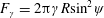 $F_{\unicode[STIX]{x1D6FE}}=2\unicode[STIX]{x03C0}\unicode[STIX]{x1D6FE}R\text{sin}^{2}\unicode[STIX]{x1D713}$
. The buoyancy force experienced by the sphere may be shown to be
$F_{\unicode[STIX]{x1D6FE}}=2\unicode[STIX]{x03C0}\unicode[STIX]{x1D6FE}R\text{sin}^{2}\unicode[STIX]{x1D713}$
. The buoyancy force experienced by the sphere may be shown to be
 $$\begin{eqnarray}F_{B}=g\{\unicode[STIX]{x1D70C}_{1}({\mathcal{V}}-{\mathcal{V}}_{spc})+\unicode[STIX]{x1D70C}_{2}{\mathcal{V}}_{spc}+(\unicode[STIX]{x1D70C}_{2}-\unicode[STIX]{x1D70C}_{1}){\mathcal{V}}_{cyl}\}.\end{eqnarray}$$
The first two contributions in (4.1) correspond to the buoyancy force that would exist if there were no meniscus,
 ${\mathcal{V}}_{spc}=(1/3)\unicode[STIX]{x03C0}R^{3}(2-3\text{cos}\unicode[STIX]{x1D713}+\text{cos}^{3}\unicode[STIX]{x1D713})$
being the volume of the spherical cap located below the plane
${\mathcal{V}}_{spc}=(1/3)\unicode[STIX]{x03C0}R^{3}(2-3\text{cos}\unicode[STIX]{x1D713}+\text{cos}^{3}\unicode[STIX]{x1D713})$
being the volume of the spherical cap located below the plane
 $z=z_{s}$
. The last contribution is due to the shift introduced by the meniscus between that plane and the undisturbed interface
$z=z_{s}$
. The last contribution is due to the shift introduced by the meniscus between that plane and the undisturbed interface
 $z=0$
. Keller (Reference Keller1998) (see also Mansfield, Sepangi & Eastwood (Reference Mansfield, Sepangi and Eastwood1997)) showed that this shift results in an additional buoyancy force proportional to the density difference
$z=0$
. Keller (Reference Keller1998) (see also Mansfield, Sepangi & Eastwood (Reference Mansfield, Sepangi and Eastwood1997)) showed that this shift results in an additional buoyancy force proportional to the density difference
 $\unicode[STIX]{x1D70C}_{2}-\unicode[STIX]{x1D70C}_{1}$
and acting on the vertical cylinder of volume
$\unicode[STIX]{x1D70C}_{2}-\unicode[STIX]{x1D70C}_{1}$
and acting on the vertical cylinder of volume
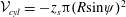 ${\mathcal{V}}_{cyl}=-z_{s}\unicode[STIX]{x03C0}(R\text{sin}\unicode[STIX]{x1D713})^{2}$
which stands on the pseudo-contact line and is limited by the above two planes. The sphere can float at the interface only if the sum of the above two forces exceeds its weight
${\mathcal{V}}_{cyl}=-z_{s}\unicode[STIX]{x03C0}(R\text{sin}\unicode[STIX]{x1D713})^{2}$
which stands on the pseudo-contact line and is limited by the above two planes. The sphere can float at the interface only if the sum of the above two forces exceeds its weight
 $F_{P}=-\unicode[STIX]{x1D70C}_{p}{\mathcal{V}}g$
. Introducing the dimensionless ‘submergence’
$F_{P}=-\unicode[STIX]{x1D70C}_{p}{\mathcal{V}}g$
. Introducing the dimensionless ‘submergence’
 $z_{s}^{\ast }=z_{s}/R$
, this condition yields the inequality
$z_{s}^{\ast }=z_{s}/R$
, this condition yields the inequality
 $$\begin{eqnarray}\frac{3}{2Bo}\text{sin}^{2}\unicode[STIX]{x1D713}-\frac{\unicode[STIX]{x1D701}_{p}}{\unicode[STIX]{x1D701}}+\frac{1}{4}(2-3\text{cos}\unicode[STIX]{x1D713}+\text{cos}^{3}\unicode[STIX]{x1D713})-\frac{3}{4}z_{s}^{\ast }\text{sin}^{2}\unicode[STIX]{x1D713}\geqslant 0.\end{eqnarray}$$

Figure 9. A sphere standing at the interface.
Evaluation of the left-hand side of (4.2) requires
 $z_{s}$
to be known as a function of
$z_{s}$
to be known as a function of
 $\unicode[STIX]{x1D713}$
, which amounts to determining the shape of the meniscus. This shape is governed by the Young–Laplace equation
$\unicode[STIX]{x1D713}$
, which amounts to determining the shape of the meniscus. This shape is governed by the Young–Laplace equation
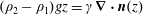 $(\unicode[STIX]{x1D70C}_{2}-\unicode[STIX]{x1D70C}_{1})gz=\unicode[STIX]{x1D6FE}\unicode[STIX]{x1D735}\boldsymbol{\cdot }\boldsymbol{n}(z)$
, where
$(\unicode[STIX]{x1D70C}_{2}-\unicode[STIX]{x1D70C}_{1})gz=\unicode[STIX]{x1D6FE}\unicode[STIX]{x1D735}\boldsymbol{\cdot }\boldsymbol{n}(z)$
, where
 $\boldsymbol{n}$
is the unit normal to the meniscus surface, subject to suitable boundary conditions. The solution of the corresponding problem can only be obtained numerically when the Bond number is finite. However, in the small-Bond-number limit, the problem was solved by O’Brien (Reference O’Brien1996), using a matched asymptotic expansion procedure directly inspired by that developed by James (Reference James1974) for a circular cylinder. In the present notation, his result for the submergence
$\boldsymbol{n}$
is the unit normal to the meniscus surface, subject to suitable boundary conditions. The solution of the corresponding problem can only be obtained numerically when the Bond number is finite. However, in the small-Bond-number limit, the problem was solved by O’Brien (Reference O’Brien1996), using a matched asymptotic expansion procedure directly inspired by that developed by James (Reference James1974) for a circular cylinder. In the present notation, his result for the submergence
 $z_{s}^{\ast }$
is written, assuming total wetting, as
$z_{s}^{\ast }$
is written, assuming total wetting, as
 $$\begin{eqnarray}\displaystyle z_{s}^{\ast }(\unicode[STIX]{x1D713})=\left(\unicode[STIX]{x1D6FE}_{E}-\text{log}\frac{4}{\sqrt{Bo}(\text{sin}\unicode[STIX]{x1D713}(1+\text{cos}\unicode[STIX]{x1D713}))}\right)\text{sin}^{2}\unicode[STIX]{x1D713}+O\left(Bo\left[\text{log}(\sqrt{Bo})\right]^{2}\right),\end{eqnarray}$$
where
 $\unicode[STIX]{x1D6FE}_{E}\simeq 0.577$
is the Euler constant. The submergence is seen to be a decreasing function of the Bond number. Indeed, for a given
$\unicode[STIX]{x1D6FE}_{E}\simeq 0.577$
is the Euler constant. The submergence is seen to be a decreasing function of the Bond number. Indeed, for a given
 $\unicode[STIX]{x1D713}$
, the smaller
$\unicode[STIX]{x1D713}$
, the smaller
 $Bo$
is the larger the energy required to bend the interface is, and hence the broader the region over which it deviates from its initial flat shape is. Inserting (4.3) into (4.2), one first has to notice that, for small Bond numbers, the most efficient configuration regarding the magnitude of positive terms on the left-hand side is reached when
$Bo$
is the larger the energy required to bend the interface is, and hence the broader the region over which it deviates from its initial flat shape is. Inserting (4.3) into (4.2), one first has to notice that, for small Bond numbers, the most efficient configuration regarding the magnitude of positive terms on the left-hand side is reached when
 $\unicode[STIX]{x1D713}=\unicode[STIX]{x03C0}/2$
. Hence, flotation is possible only for spheres such that
$\unicode[STIX]{x1D713}=\unicode[STIX]{x03C0}/2$
. Hence, flotation is possible only for spheres such that
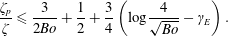 $$\begin{eqnarray}\frac{\unicode[STIX]{x1D701}_{p}}{\unicode[STIX]{x1D701}}\leqslant \frac{3}{2Bo}+\frac{1}{2}+\frac{3}{4}\left(\text{log}\frac{4}{\sqrt{Bo}}-\unicode[STIX]{x1D6FE}_{E}\right).\end{eqnarray}$$
The leading-order term on the right-hand side is identical to that obtained by Vella et al. (Reference Vella, Lee and Kim2006), still in the low-Bond-number limit. It is worth noting that comparison of the submergence determined by solving the exact Young–Laplace problem numerically (see PM2) with the low-
 $Bo$
asymptotic prediction (4.3) reveals that the latter (hence the flotation criterion (4.4)) remains a valid approximation up to
$Bo$
asymptotic prediction (4.3) reveals that the latter (hence the flotation criterion (4.4)) remains a valid approximation up to
 $Bo=O(1)$
: for
$Bo=O(1)$
: for
 $Bo=1$
, (4.3) overestimates the submergence by
$Bo=1$
, (4.3) overestimates the submergence by
 $20\,\%$
, so that (4.4) overestimates the critical
$20\,\%$
, so that (4.4) overestimates the critical
 $\unicode[STIX]{x1D701}_{p}/\unicode[STIX]{x1D701}$
only by
$\unicode[STIX]{x1D701}_{p}/\unicode[STIX]{x1D701}$
only by
 $6\,\%$
.
$6\,\%$
.
It must be stressed that (4.4) only provides a necessary condition for flotation to be possible. As it was derived in the framework of a strictly static approach, it is unable to account for the influence of any initial sphere motion, which is expected to lower the critical density ratio, allowing the sphere to float, i.e. its velocity to vanish before the meniscus snaps. Incorporation of dynamic effects requires the viscous drag acting on the sphere to be evaluated. This was empirically achieved by Lee & Kim (Reference Lee and Kim2011) in the case of a sphere crossing a gas–liquid interface, by considering that the local velocity and pressure distributions over the part of the sphere surface immersed in the liquid are identical to those found in the Stokes flow past a sphere settling in an unbounded fluid. Extension of this approach to the present two-fluid problem is appealing, but the viscosity contrast would generate a pressure jump across the interface, making the conclusions doubtful.
For finite Bond numbers, the shape of the meniscus can only be determined through a numerical solution of the Young–Laplace problem. Nevertheless, a rough model assuming that the meniscus takes the form of an arc of a circle with a radius
 $r_{\unicode[STIX]{x1D713}}$
has been derived to evaluate the minimum size allowing rigid spheres or gas bubbles to fall or rise across an interface (Maru et al.
Reference Maru, Wasan and Kintner1971; Bonhomme et al.
Reference Bonhomme, Magnaudet, Duval and Piar2012). The requirement that the meniscus be tangent to the sphere on the plane
$r_{\unicode[STIX]{x1D713}}$
has been derived to evaluate the minimum size allowing rigid spheres or gas bubbles to fall or rise across an interface (Maru et al.
Reference Maru, Wasan and Kintner1971; Bonhomme et al.
Reference Bonhomme, Magnaudet, Duval and Piar2012). The requirement that the meniscus be tangent to the sphere on the plane
 $z=z_{s}$
as well as on the undisturbed interface yields
$z=z_{s}$
as well as on the undisturbed interface yields
 $r_{\unicode[STIX]{x1D713}}=\{-1+[1+4Bo(1-\cos \unicode[STIX]{x1D713})]^{1/2}\}\{2Bo(1-\cos \unicode[STIX]{x1D713})\}^{-1}$
, from which the submergence
$r_{\unicode[STIX]{x1D713}}=\{-1+[1+4Bo(1-\cos \unicode[STIX]{x1D713})]^{1/2}\}\{2Bo(1-\cos \unicode[STIX]{x1D713})\}^{-1}$
, from which the submergence
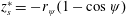 $z_{s}^{\ast }=-r_{\unicode[STIX]{x1D713}}(1-\cos \unicode[STIX]{x1D713})$
is obtained. In the limit of large Bond numbers, this model predicts
$z_{s}^{\ast }=-r_{\unicode[STIX]{x1D713}}(1-\cos \unicode[STIX]{x1D713})$
is obtained. In the limit of large Bond numbers, this model predicts
 $z_{s}^{\ast }\propto Bo^{-1/2}$
, so that the dominant terms in (4.2) are now those due to the buoyancy force. Consequently, the cap angle
$z_{s}^{\ast }\propto Bo^{-1/2}$
, so that the dominant terms in (4.2) are now those due to the buoyancy force. Consequently, the cap angle
 $\unicode[STIX]{x1D713}_{max}$
at which this force is maximum is close to
$\unicode[STIX]{x1D713}_{max}$
at which this force is maximum is close to
 $\unicode[STIX]{x03C0}$
. More precisely, one finds
$\unicode[STIX]{x03C0}$
. More precisely, one finds
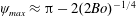 $\unicode[STIX]{x1D713}_{max}\approx \unicode[STIX]{x03C0}-2(2Bo)^{-1/4}$
, for which
$\unicode[STIX]{x1D713}_{max}\approx \unicode[STIX]{x03C0}-2(2Bo)^{-1/4}$
, for which
 $z_{s}^{\ast }\approx -(2/Bo)^{1/2}$
. It should be noted that the column enclosed within the meniscus is very thin under such conditions (its minimum dimensionless radius is
$z_{s}^{\ast }\approx -(2/Bo)^{1/2}$
. It should be noted that the column enclosed within the meniscus is very thin under such conditions (its minimum dimensionless radius is
 $2(2Bo)^{-1/4}$
), but pinch-off is not reached yet. Use of these results in (4.2) yields the approximate flotation condition
$2(2Bo)^{-1/4}$
), but pinch-off is not reached yet. Use of these results in (4.2) yields the approximate flotation condition
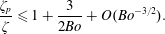 $$\begin{eqnarray}\frac{\unicode[STIX]{x1D701}_{p}}{\unicode[STIX]{x1D701}}\leqslant 1+\frac{3}{2Bo}+O(Bo^{-3/2}).\end{eqnarray}$$
The criteria (4.4) and (4.5) coincide for
 $Bo\approx 2.5$
. Fortuitously, the prefactor of the
$Bo\approx 2.5$
. Fortuitously, the prefactor of the
 $Bo^{-1}$
term is the same in both of them. Hence, as may be seen in figure 10, there is not much difference between the two predictions in the low-
$Bo^{-1}$
term is the same in both of them. Hence, as may be seen in figure 10, there is not much difference between the two predictions in the low-
 $Bo$
range, although (4.5) is not expected to be valid there.
$Bo$
range, although (4.5) is not expected to be valid there.
4.2 Observations versus model predictions
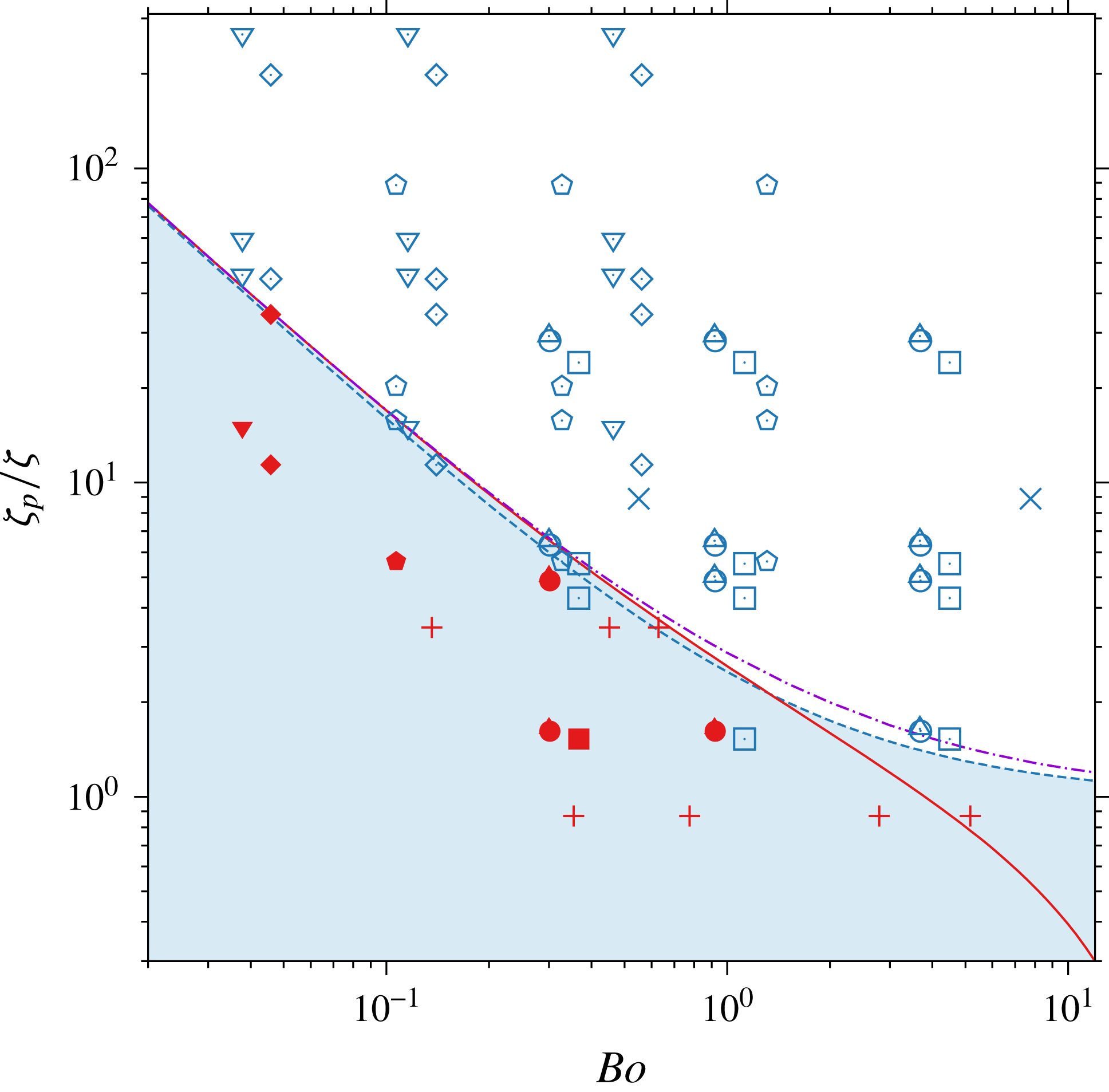
Figure 10. The configurations reached by spheres settling in various pairs of fluids in the
 $(\unicode[STIX]{x1D701}_{p}/\unicode[STIX]{x1D701}=(\unicode[STIX]{x1D70C}_{p}-\unicode[STIX]{x1D70C}_{1})/(\unicode[STIX]{x1D70C}_{2}-\unicode[STIX]{x1D70C}_{1}),Bo=(\unicode[STIX]{x1D70C}_{2}-\unicode[STIX]{x1D70C}_{1})gR^{2}/\unicode[STIX]{x1D6FE})$
plane. Closed (respectively open) symbols refer to cases in which the sphere floats at (respectively crosses) the interface. Solid line, low-
$(\unicode[STIX]{x1D701}_{p}/\unicode[STIX]{x1D701}=(\unicode[STIX]{x1D70C}_{p}-\unicode[STIX]{x1D70C}_{1})/(\unicode[STIX]{x1D70C}_{2}-\unicode[STIX]{x1D70C}_{1}),Bo=(\unicode[STIX]{x1D70C}_{2}-\unicode[STIX]{x1D70C}_{1})gR^{2}/\unicode[STIX]{x1D6FE})$
plane. Closed (respectively open) symbols refer to cases in which the sphere floats at (respectively crosses) the interface. Solid line, low-
 $Bo$
criterion (4.4); dashed line, high-
$Bo$
criterion (4.4); dashed line, high-
 $Bo$
criterion (4.5); dash-dotted line, exact solution of the Young–Laplace problem; squares, V5/water–glycerin; circles, V50/water–glycerin; triangles (up), V500/water–glycerin; pentagons, V5/water; diamonds, V50/water; triangles (down), V500/water. Data from Maru et al. (Reference Maru, Wasan and Kintner1971) corresponding to
$Bo$
criterion (4.5); dash-dotted line, exact solution of the Young–Laplace problem; squares, V5/water–glycerin; circles, V50/water–glycerin; triangles (up), V500/water–glycerin; pentagons, V5/water; diamonds, V50/water; triangles (down), V500/water. Data from Maru et al. (Reference Maru, Wasan and Kintner1971) corresponding to
 $+$
, floating conditions (plexiglas and Teflon spheres in a mineral oil/water-
$+$
, floating conditions (plexiglas and Teflon spheres in a mineral oil/water-
 $96\,\%$
glycerin set-up);
$96\,\%$
glycerin set-up);
 $\times$
, breakthrough conditions (glass spheres in a cyclohexanol/water-
$\times$
, breakthrough conditions (glass spheres in a cyclohexanol/water-
 $62\,\%$
glycerin set-up).
$62\,\%$
glycerin set-up).
Figure 10 gathers observations performed in the six pairs of fluids in which, depending on the sphere density and size, either flotation or tailing configurations were noticed. Some data recorded by Maru et al. (Reference Maru, Wasan and Kintner1971) have also been included. Not surprisingly, the shape of the frontier separating the two regimes is qualitatively similar to that drawn in the phase diagram of figure 6. In addition to the approximate criteria (4.4) and (4.5), we also plot the prediction obtained by solving the Young–Laplace equation numerically throughout the whole range of Bond numbers (the corresponding numerical procedure is described in appendix B of PM2). This numerical solution allowed us to obtain the submergence
 $z_{s}^{\ast }(\unicode[STIX]{x1D713},Bo)$
for arbitrary values of
$z_{s}^{\ast }(\unicode[STIX]{x1D713},Bo)$
for arbitrary values of
 $\unicode[STIX]{x1D713}$
. With this information at hand, we could determine the optimum cap angle
$\unicode[STIX]{x1D713}$
. With this information at hand, we could determine the optimum cap angle
 $\unicode[STIX]{x1D713}_{o}(Bo)$
maximizing
$\unicode[STIX]{x1D713}_{o}(Bo)$
maximizing
 $\unicode[STIX]{x1D701}_{p}/\unicode[STIX]{x1D701}$
in the inequality (4.2) for each value of
$\unicode[STIX]{x1D701}_{p}/\unicode[STIX]{x1D701}$
in the inequality (4.2) for each value of
 $Bo$
(
$Bo$
(
 $\unicode[STIX]{x1D713}_{o}(Bo)$
ranges from
$\unicode[STIX]{x1D713}_{o}(Bo)$
ranges from
 $\unicode[STIX]{x03C0}/2$
for
$\unicode[STIX]{x03C0}/2$
for
 $Bo\lesssim 1$
to approximately
$Bo\lesssim 1$
to approximately
 $3\unicode[STIX]{x03C0}/4$
for
$3\unicode[STIX]{x03C0}/4$
for
 $Bo=10$
). The difference between this exact prediction and those provided by the approximate criteria is clearly small, with a maximum of approximately
$Bo=10$
). The difference between this exact prediction and those provided by the approximate criteria is clearly small, with a maximum of approximately
 $15\,\%$
in the range
$15\,\%$
in the range
 $1.5\lesssim Bo\lesssim 3$
. Overall, the behaviour observed in experiments is consistent with the theoretical predictions. Not surprisingly, some experiments corresponding to conditions located slightly below the critical curve provided by (4.4) resulted in a tailing configuration. They may be considered as a confirmation of the fact that the above two criteria only provide a necessary condition for flotation to be possible. However, experimental uncertainty regarding the interfacial tension may also play some role, since it is directly reflected in the critical value of
$1.5\lesssim Bo\lesssim 3$
. Overall, the behaviour observed in experiments is consistent with the theoretical predictions. Not surprisingly, some experiments corresponding to conditions located slightly below the critical curve provided by (4.4) resulted in a tailing configuration. They may be considered as a confirmation of the fact that the above two criteria only provide a necessary condition for flotation to be possible. However, experimental uncertainty regarding the interfacial tension may also play some role, since it is directly reflected in the critical value of
 $\unicode[STIX]{x1D701}_{p}/\unicode[STIX]{x1D701}$
. Departures from the total wetting assumption may also have also some influence in these marginal cases: if the meniscus makes a finite angle, say
$\unicode[STIX]{x1D701}_{p}/\unicode[STIX]{x1D701}$
. Departures from the total wetting assumption may also have also some influence in these marginal cases: if the meniscus makes a finite angle, say
 $\unicode[STIX]{x1D6F7}$
, with the tangent to the sphere at the pseudo-contact line, it is readily shown that the
$\unicode[STIX]{x1D6F7}$
, with the tangent to the sphere at the pseudo-contact line, it is readily shown that the
 $\sin ^{2}\unicode[STIX]{x1D713}$
factor in front of the first term on the right-hand sides of (4.2) and (4.3) is changed into
$\sin ^{2}\unicode[STIX]{x1D713}$
factor in front of the first term on the right-hand sides of (4.2) and (4.3) is changed into
 $\sin \unicode[STIX]{x1D713}\sin (\unicode[STIX]{x1D713}-\unicode[STIX]{x1D6F7})$
, whereas the
$\sin \unicode[STIX]{x1D713}\sin (\unicode[STIX]{x1D713}-\unicode[STIX]{x1D6F7})$
, whereas the
 $\cos \unicode[STIX]{x1D713}$
term in (4.3) is changed into
$\cos \unicode[STIX]{x1D713}$
term in (4.3) is changed into
 $\cos (\unicode[STIX]{x1D713}-\unicode[STIX]{x1D6F7})$
. For small
$\cos (\unicode[STIX]{x1D713}-\unicode[STIX]{x1D6F7})$
. For small
 $Bo$
, the total buoyancy force sustaining the sphere is then maximized when
$Bo$
, the total buoyancy force sustaining the sphere is then maximized when
 $\unicode[STIX]{x1D713}\approx \unicode[STIX]{x03C0}/2+\unicode[STIX]{x1D6F7}/2$
instead of
$\unicode[STIX]{x1D713}\approx \unicode[STIX]{x03C0}/2+\unicode[STIX]{x1D6F7}/2$
instead of
 $\unicode[STIX]{x1D713}=\unicode[STIX]{x03C0}/2$
, so that its dominant contribution is reduced by a factor of
$\unicode[STIX]{x1D713}=\unicode[STIX]{x03C0}/2$
, so that its dominant contribution is reduced by a factor of
 $(1/2)\cos ^{2}\unicode[STIX]{x1D6F7}$
.
$(1/2)\cos ^{2}\unicode[STIX]{x1D6F7}$
.
Two situations observed in the V5/water–glycerin pair may be noticed to lead to tailing configurations, although the corresponding values of
 $\unicode[STIX]{x1D701}_{p}/\unicode[STIX]{x1D701}$
clearly satisfy (4.4). These are the two points
$\unicode[STIX]{x1D701}_{p}/\unicode[STIX]{x1D701}$
clearly satisfy (4.4). These are the two points
 $Bo=0.37$
,
$Bo=0.37$
,
 $\unicode[STIX]{x1D701}_{p}/\unicode[STIX]{x1D701}=4.29$
and
$\unicode[STIX]{x1D701}_{p}/\unicode[STIX]{x1D701}=4.29$
and
 $Bo=1.12$
,
$Bo=1.12$
,
 $\unicode[STIX]{x1D701}_{p}/\unicode[STIX]{x1D701}=1.53$
in figure 10. The latter, which is analysed in detail in PM2 with the help of numerical simulations, corresponds to configuration 13
$\unicode[STIX]{x1D701}_{p}/\unicode[STIX]{x1D701}=1.53$
in figure 10. The latter, which is analysed in detail in PM2 with the help of numerical simulations, corresponds to configuration 13
 $a$
in figure 4(a), which was seen to experience a quasi-steady detachment. It is of interest to notice that, among the various combinations of fluids we employed, the V5/water–glycerin pair is the one in which inertia effects induced by the sphere motion are the largest in the upper fluid, and deformation of the interface is the most energy-consuming, due to the large viscosity ratio (
$a$
in figure 4(a), which was seen to experience a quasi-steady detachment. It is of interest to notice that, among the various combinations of fluids we employed, the V5/water–glycerin pair is the one in which inertia effects induced by the sphere motion are the largest in the upper fluid, and deformation of the interface is the most energy-consuming, due to the large viscosity ratio (
 $\unicode[STIX]{x1D706}=18.3$
) and the significant fluid density contrast (
$\unicode[STIX]{x1D706}=18.3$
) and the significant fluid density contrast (
 $\unicode[STIX]{x1D701}=0.32$
). Consequently, the deceleration experienced by the sphere when it reaches the interface is maximum in this pair of fluids, and one can expect the corresponding dynamical effects to deeply alter the quasi-static force balance (4.2), and hence the flotation criterion (4.4).
$\unicode[STIX]{x1D701}=0.32$
). Consequently, the deceleration experienced by the sphere when it reaches the interface is maximum in this pair of fluids, and one can expect the corresponding dynamical effects to deeply alter the quasi-static force balance (4.2), and hence the flotation criterion (4.4).
4.3 How do dynamical effects alter the static balance?
The qualitative picture of these effects is as follows. The sphere velocity in the upper fluid is of
 $O((\unicode[STIX]{x1D701}_{p}gR)^{1/2})$
and the sphere almost comes to rest within a distance of
$O((\unicode[STIX]{x1D701}_{p}gR)^{1/2})$
and the sphere almost comes to rest within a distance of
 $O(R)$
when it reaches the interface. Hence, it undergoes a negative acceleration
$O(R)$
when it reaches the interface. Hence, it undergoes a negative acceleration
 $\text{d}V/\text{d}t=V\,\text{d}V/\text{d}z$
which is initially of
$\text{d}V/\text{d}t=V\,\text{d}V/\text{d}z$
which is initially of
 $O(\unicode[STIX]{x1D701}_{p}g)$
and produces a downward inertia force
$O(\unicode[STIX]{x1D701}_{p}g)$
and produces a downward inertia force
 $-(4/3)\unicode[STIX]{x03C0}R^{3}(\unicode[STIX]{x1D70C}_{p}+\unicode[STIX]{x1D70C}_{1}C_{M}(t))\,\text{d}V/\text{d}t$
, where
$-(4/3)\unicode[STIX]{x03C0}R^{3}(\unicode[STIX]{x1D70C}_{p}+\unicode[STIX]{x1D70C}_{1}C_{M}(t))\,\text{d}V/\text{d}t$
, where
 $C_{M}(t)$
denotes the added-mass coefficient. In the present situation, this coefficient depends on time, increasing as the sphere gets closer to the interface (Milne-Thomson Reference Milne-Thomson1962). This inertia force provides an additional dimensionless contribution of the order of
$C_{M}(t)$
denotes the added-mass coefficient. In the present situation, this coefficient depends on time, increasing as the sphere gets closer to the interface (Milne-Thomson Reference Milne-Thomson1962). This inertia force provides an additional dimensionless contribution of the order of
 $-(\unicode[STIX]{x1D701}_{p}+1+C_{M}(t))\unicode[STIX]{x1D701}_{p}/\unicode[STIX]{x1D701}$
on the left-hand side of (4.2). The magnitude of this force decreases as the sphere decelerates and is reduced to a fraction of its initial value by the time the sphere velocity vanishes (which happens for
$-(\unicode[STIX]{x1D701}_{p}+1+C_{M}(t))\unicode[STIX]{x1D701}_{p}/\unicode[STIX]{x1D701}$
on the left-hand side of (4.2). The magnitude of this force decreases as the sphere decelerates and is reduced to a fraction of its initial value by the time the sphere velocity vanishes (which happens for
 $\unicode[STIX]{x1D713}\approx \unicode[STIX]{x03C0}/2$
, as figures 3(c) and (j) of PM2 show). However, a ‘history’ force, qualitatively similar to the Boussinesq–Basset force in the low-Reynolds-number regime, has taken over in the meantime. This force is due to the downthrust produced by the progressive collapse of the sphere wake. At time
$\unicode[STIX]{x1D713}\approx \unicode[STIX]{x03C0}/2$
, as figures 3(c) and (j) of PM2 show). However, a ‘history’ force, qualitatively similar to the Boussinesq–Basset force in the low-Reynolds-number regime, has taken over in the meantime. This force is due to the downthrust produced by the progressive collapse of the sphere wake. At time
 $t$
, it depends on the cumulated changes induced by the deceleration on the wake over previous times through a kernel
$t$
, it depends on the cumulated changes induced by the deceleration on the wake over previous times through a kernel
 $K(t-\unicode[STIX]{x1D70F})$
, with
$K(t-\unicode[STIX]{x1D70F})$
, with
 $-\infty \leqslant \unicode[STIX]{x1D70F}\leqslant t$
. This kernel is inertial by nature in the present situation where
$-\infty \leqslant \unicode[STIX]{x1D70F}\leqslant t$
. This kernel is inertial by nature in the present situation where
 $Ar\gg 1$
, since wake disturbances are advected with the velocity
$Ar\gg 1$
, since wake disturbances are advected with the velocity
 $V\gg \unicode[STIX]{x1D707}_{1}/(\unicode[STIX]{x1D70C}_{1}R)$
. The closely related situation of a sudden stop of the sphere at
$V\gg \unicode[STIX]{x1D707}_{1}/(\unicode[STIX]{x1D70C}_{1}R)$
. The closely related situation of a sudden stop of the sphere at
 $t=0$
was considered by Lovalenti & Brady (Reference Lovalenti and Brady1993) in the Oseen regime. They showed that the corresponding ‘history’ effect results in a force that reduces the net drag and is written at leading order as
$t=0$
was considered by Lovalenti & Brady (Reference Lovalenti and Brady1993) in the Oseen regime. They showed that the corresponding ‘history’ effect results in a force that reduces the net drag and is written at leading order as
 $6\unicode[STIX]{x03C0}\unicode[STIX]{x1D707}_{1}RV[(3/4)R(Vt)^{-1}]=(9/2)\unicode[STIX]{x03C0}\unicode[STIX]{x1D707}_{1}R^{2}t^{-1}$
. This prediction was extended to arbitrary Reynolds number by Lawrence & Mei (Reference Lawrence and Mei1995). Their analysis, confirmed by numerical simulations, showed that the ratio of the ‘history’ contribution to the steady drag at the corresponding Reynolds number is still
$6\unicode[STIX]{x03C0}\unicode[STIX]{x1D707}_{1}RV[(3/4)R(Vt)^{-1}]=(9/2)\unicode[STIX]{x03C0}\unicode[STIX]{x1D707}_{1}R^{2}t^{-1}$
. This prediction was extended to arbitrary Reynolds number by Lawrence & Mei (Reference Lawrence and Mei1995). Their analysis, confirmed by numerical simulations, showed that the ratio of the ‘history’ contribution to the steady drag at the corresponding Reynolds number is still
 $-(3/4)R(|V|t)^{-1}$
. Here, the steady drag balances the net weight of the sphere in the upper fluid, so that the contribution of the ‘history’ effect to the left-hand side of (4.2) in the case of a sudden stop would be
$-(3/4)R(|V|t)^{-1}$
. Here, the steady drag balances the net weight of the sphere in the upper fluid, so that the contribution of the ‘history’ effect to the left-hand side of (4.2) in the case of a sudden stop would be
 $-(3/4)R(|V|t)^{-1}\unicode[STIX]{x1D701}_{p}/\unicode[STIX]{x1D701}$
, i.e. it would be of
$-(3/4)R(|V|t)^{-1}\unicode[STIX]{x1D701}_{p}/\unicode[STIX]{x1D701}$
, i.e. it would be of
 $O(\unicode[STIX]{x1D701}_{p}/\unicode[STIX]{x1D701})$
over a time period of
$O(\unicode[STIX]{x1D701}_{p}/\unicode[STIX]{x1D701})$
over a time period of
 $O(R/|V|)=O(\{R/(\unicode[STIX]{x1D701}_{p}g)\}^{1/2})$
. Although the sphere does not experience a strict sudden stop in the present experiments, the characteristic time
$O(R/|V|)=O(\{R/(\unicode[STIX]{x1D701}_{p}g)\}^{1/2})$
. Although the sphere does not experience a strict sudden stop in the present experiments, the characteristic time
 $(R/(\unicode[STIX]{x1D701}_{p}g))^{1/2}$
is much smaller than the viscous time scale
$(R/(\unicode[STIX]{x1D701}_{p}g))^{1/2}$
is much smaller than the viscous time scale
 $\unicode[STIX]{x1D70C}_{1}R^{2}/\unicode[STIX]{x1D707}_{1}$
, making the sudden stop model qualitatively relevant.
$\unicode[STIX]{x1D70C}_{1}R^{2}/\unicode[STIX]{x1D707}_{1}$
, making the sudden stop model qualitatively relevant.
To summarize, the above analysis shows that in situations where the stopping of the sphere takes place over an
 $O(R)$
distance, which is the case when
$O(R)$
distance, which is the case when
 $Ar\gg 1$
and
$Ar\gg 1$
and
 $\unicode[STIX]{x1D706}\gg 1$
, the various inertia effects due to this stopping result in an additional negative contribution proportional to
$\unicode[STIX]{x1D706}\gg 1$
, the various inertia effects due to this stopping result in an additional negative contribution proportional to
 $\unicode[STIX]{x1D701}_{p}/\unicode[STIX]{x1D701}$
on the left-hand side of (4.4). As the prefactor of this contribution is of
$\unicode[STIX]{x1D701}_{p}/\unicode[STIX]{x1D701}$
on the left-hand side of (4.4). As the prefactor of this contribution is of
 $O(1)$
during the entire deceleration stage and even during some time after the sphere velocity has almost vanished, due to the
$O(1)$
during the entire deceleration stage and even during some time after the sphere velocity has almost vanished, due to the
 $t^{-1}$
decay of the ‘history’ force, the actual critical density ratio below which the sphere can float is reduced by a factor of the order of 2 when
$t^{-1}$
decay of the ‘history’ force, the actual critical density ratio below which the sphere can float is reduced by a factor of the order of 2 when
 $\unicode[STIX]{x1D713}=\unicode[STIX]{x03C0}/2$
compared with the prediction (4.4). Under such conditions, it is clear that the aforementioned two spheres released in the V5/water–glycerin pair cannot float. According to figure 10, the only sphere that is observed to float in this pair of fluids is the smallest polyacetal sphere (configuration 10(a) in figure 4(a)) with
$\unicode[STIX]{x1D713}=\unicode[STIX]{x03C0}/2$
compared with the prediction (4.4). Under such conditions, it is clear that the aforementioned two spheres released in the V5/water–glycerin pair cannot float. According to figure 10, the only sphere that is observed to float in this pair of fluids is the smallest polyacetal sphere (configuration 10(a) in figure 4(a)) with
 $Bo=0.36$
and
$Bo=0.36$
and
 $\unicode[STIX]{x1D701}_{p}/\unicode[STIX]{x1D701}=1.57$
, a density ratio nearly four times smaller than the critical value predicted by the static criterion (4.4).
$\unicode[STIX]{x1D701}_{p}/\unicode[STIX]{x1D701}=1.57$
, a density ratio nearly four times smaller than the critical value predicted by the static criterion (4.4).
5 How does the volume of attached drops scale?

Figure 11. The post-pinch-off evolution of the attached drop past a
 $R=7$
mm polyacetal sphere in the V50/water–glycerin system (configuration
$R=7$
mm polyacetal sphere in the V50/water–glycerin system (configuration
 $7a$
,
$7a$
,
 $\unicode[STIX]{x1D706}=1.7,\unicode[STIX]{x1D701}=0.26$
).
$\unicode[STIX]{x1D706}=1.7,\unicode[STIX]{x1D701}=0.26$
).

Figure 12. Some compound sphere + drop bodies. (a–c) In the V5/water + glycerin system (
 $\unicode[STIX]{x1D706}=18.3,\unicode[STIX]{x1D701}=0.32$
) with (a) an
$\unicode[STIX]{x1D706}=18.3,\unicode[STIX]{x1D701}=0.32$
) with (a) an
 $R=2$
mm aluminium sphere, (b) an
$R=2$
mm aluminium sphere, (b) an
 $R=3.5$
mm glass sphere (configuration
$R=3.5$
mm glass sphere (configuration
 $14a$
) and (c) an
$14a$
) and (c) an
 $R=7$
mm polyacetal sphere (configuration
$R=7$
mm polyacetal sphere (configuration
 $16a$
); (d–f) in the V500/water system (
$16a$
); (d–f) in the V500/water system (
 $\unicode[STIX]{x1D706}=1.9\times 10^{-3},\unicode[STIX]{x1D701}=2.7\times 10^{-2}$
) with (d) an
$\unicode[STIX]{x1D706}=1.9\times 10^{-3},\unicode[STIX]{x1D701}=2.7\times 10^{-2}$
) with (d) an
 $R=2$
mm aluminium sphere, (e) an
$R=2$
mm aluminium sphere, (e) an
 $R=3.5$
mm aluminium sphere and (f) an
$R=3.5$
mm aluminium sphere and (f) an
 $R=5$
mm polyacetal sphere.
$R=5$
mm polyacetal sphere.
In the quasi-static detachment and tailing regimes, after the meniscus has snapped or the tail has pinched off, a certain amount of light fluid recedes towards the sphere, resulting eventually in a drop that remains attached to its upper part. Figure 11 shows a typical post-pinch-off evolution of the interface separating the outer fluid from the volume of light fluid enclosing the sphere. The film that covers the front half of the sphere thins down over most of the sequence, bringing fluid towards the rear half, hence increasing the drop volume. Clearly, there is a significant interaction between the film and the drop through this mass exchange during this transient. Simultaneously, the drop lengthens and its curvature at the apex increases, due to the shearing by the outer flow. This shearing process takes a significant time in the present example because the two fluids have similar viscosities; it is much longer when
 $\unicode[STIX]{x1D706}\ll 1$
, so that the drop evolves very slowly and may not have reached a strictly final shape at the end of the observations. The corresponding transient is much shorter when
$\unicode[STIX]{x1D706}\ll 1$
, so that the drop evolves very slowly and may not have reached a strictly final shape at the end of the observations. The corresponding transient is much shorter when
 $\unicode[STIX]{x1D706}$
is large. Since there is virtually no shear at the drop/outer-fluid interface in that case, this transient corresponds to the time required for the normal stress distribution at the drop surface to develop.
$\unicode[STIX]{x1D706}$
is large. Since there is virtually no shear at the drop/outer-fluid interface in that case, this transient corresponds to the time required for the normal stress distribution at the drop surface to develop.
Some examples of the observed drops, once they have reached their final or quasi-final shape, are displayed in figure 12. Those in figure 12(a–c) have quite prolate shapes, whereas those in figure 12(d–f) are roughly spherical. Moreover, the volume of the latter is much larger, and may in some cases be of the same order as or even larger than that of the sphere (e.g. figure 12(e)); in such cases, the drop entirely covers the upper half of the sphere. One should note the differences between 12(a) and (d), which correspond to the same sphere but were taken in different fluid pairs, underlining the strong influence of the density and viscosity contrasts (both pairs have similar interfacial tensions).
5.1 Overall force balances
Theoretical determination of the final drop volume, say
 ${\mathcal{V}}_{d}$
, under general conditions is a very complex free-boundary problem which is beyond the scope of this study. Nevertheless, the wide range of conditions covered in the present experiments makes it desirable to develop a qualitative understanding of the influence of the various flow parameters on
${\mathcal{V}}_{d}$
, under general conditions is a very complex free-boundary problem which is beyond the scope of this study. Nevertheless, the wide range of conditions covered in the present experiments makes it desirable to develop a qualitative understanding of the influence of the various flow parameters on
 ${\mathcal{V}}_{d}$
. Previous studies of this problem have focused on strictly static aspects by solving the Young–Laplace equation in order to determine the shape of the interface for a given drop volume (Shoukry, Hafez & Hartland Reference Shoukry, Hafez and Hartland1975; Smith & Van de Den Reference Smith and Van de Den1985). However, other effects come into play when the sphere moves, due to the fluid motion within and around the drop, as the transient stage described by figure 11 makes clear. Such effects were first considered theoretically by Johnson (Reference Johnson1981) in the limit of thin drops, but buoyancy effects were not included. Here, to better understand the consequences of the sphere motion on the volume of entrained drops, we use as a guide the stationary force balance on the compound ‘sphere
${\mathcal{V}}_{d}$
. Previous studies of this problem have focused on strictly static aspects by solving the Young–Laplace equation in order to determine the shape of the interface for a given drop volume (Shoukry, Hafez & Hartland Reference Shoukry, Hafez and Hartland1975; Smith & Van de Den Reference Smith and Van de Den1985). However, other effects come into play when the sphere moves, due to the fluid motion within and around the drop, as the transient stage described by figure 11 makes clear. Such effects were first considered theoretically by Johnson (Reference Johnson1981) in the limit of thin drops, but buoyancy effects were not included. Here, to better understand the consequences of the sphere motion on the volume of entrained drops, we use as a guide the stationary force balance on the compound ‘sphere
 $+$
drop’ body, and on the attached drop itself.
$+$
drop’ body, and on the attached drop itself.
We establish these balances in the limit of vanishingly small inertia effects (
 $Ar\ll 1$
). The drag force acting on the compound body settling with velocity
$Ar\ll 1$
). The drag force acting on the compound body settling with velocity
 $V$
may be written in the form
$V$
may be written in the form
 $F_{D}=-6\unicode[STIX]{x03C0}\unicode[STIX]{x1D707}_{2}(1+K)RV$
, where
$F_{D}=-6\unicode[STIX]{x03C0}\unicode[STIX]{x1D707}_{2}(1+K)RV$
, where
 $K$
is a correction factor to Stokes’ law resulting from the prolate geometry induced by the presence of the drop (which tends to increase the drag) and influenced by the recirculating flow within it, which can be significant if
$K$
is a correction factor to Stokes’ law resulting from the prolate geometry induced by the presence of the drop (which tends to increase the drag) and influenced by the recirculating flow within it, which can be significant if
 $\unicode[STIX]{x1D706}$
is of
$\unicode[STIX]{x1D706}$
is of
 $O(1)$
or larger and may even decrease the overall drag if
$O(1)$
or larger and may even decrease the overall drag if
 $\unicode[STIX]{x1D706}$
is large enough (Johnson Reference Johnson1981). Taking into account the weight and buoyancy forces yields at equilibrium
$\unicode[STIX]{x1D706}$
is large enough (Johnson Reference Johnson1981). Taking into account the weight and buoyancy forces yields at equilibrium
 $$\begin{eqnarray}\unicode[STIX]{x1D70C}_{2}({\mathcal{V}}+{\mathcal{V}}_{d})g-(\unicode[STIX]{x1D70C}_{p}{\mathcal{V}}+\unicode[STIX]{x1D70C}_{1}{\mathcal{V}}_{d})g-6\unicode[STIX]{x03C0}\unicode[STIX]{x1D707}_{2}(1+K)RV=0.\end{eqnarray}$$
Let us now examine the force balance on the drop itself. We assume that the drop no longer interacts with the thin film that still coats the sphere in the region located ahead of the cap angle
 $\unicode[STIX]{x1D719}=\unicode[STIX]{x1D719}_{d}$
(with
$\unicode[STIX]{x1D719}=\unicode[STIX]{x1D719}_{d}$
(with
 $\unicode[STIX]{x1D719}=0$
at the top of the sphere). Although there is no strict contact line there, this position corresponds to a pseudo-contact line where the tangent to the drop/outer-fluid interface makes a finite angle
$\unicode[STIX]{x1D719}=0$
at the top of the sphere). Although there is no strict contact line there, this position corresponds to a pseudo-contact line where the tangent to the drop/outer-fluid interface makes a finite angle
 $\unicode[STIX]{x1D6F7}$
with the sphere surface, as figure 13 shows. Interfacial tension induces a net downward force at
$\unicode[STIX]{x1D6F7}$
with the sphere surface, as figure 13 shows. Interfacial tension induces a net downward force at
 $\unicode[STIX]{x1D719}=\unicode[STIX]{x1D719}_{d}$
, the vertical component of which is
$\unicode[STIX]{x1D719}=\unicode[STIX]{x1D719}_{d}$
, the vertical component of which is
 $F_{\unicode[STIX]{x1D6FE}_{C}}=-2\unicode[STIX]{x03C0}\unicode[STIX]{x1D6FE}R\sin \unicode[STIX]{x1D719}_{d}\sin (\unicode[STIX]{x1D719}_{d}+\unicode[STIX]{x1D6F7})$
. The hydrostatic pressure component acting over the drop surface yields the usual buoyancy force
$F_{\unicode[STIX]{x1D6FE}_{C}}=-2\unicode[STIX]{x03C0}\unicode[STIX]{x1D6FE}R\sin \unicode[STIX]{x1D719}_{d}\sin (\unicode[STIX]{x1D719}_{d}+\unicode[STIX]{x1D6F7})$
. The hydrostatic pressure component acting over the drop surface yields the usual buoyancy force
 $F_{B}=g(\unicode[STIX]{x1D70C}_{2}-\unicode[STIX]{x1D70C}_{1}){\mathcal{V}}_{d}$
. However, the drop/sphere interface also contributes to the overall balance though capillary and hydrostatic effects. Introducing the radius of curvature,
$F_{B}=g(\unicode[STIX]{x1D70C}_{2}-\unicode[STIX]{x1D70C}_{1}){\mathcal{V}}_{d}$
. However, the drop/sphere interface also contributes to the overall balance though capillary and hydrostatic effects. Introducing the radius of curvature,
 $R_{0}$
, of the drop at its apex, and the distance,
$R_{0}$
, of the drop at its apex, and the distance,
 $h_{0}$
, from the apex to the top of the sphere (see figure 13), it is readily shown that the corresponding contribution yields a net vertical force with an upward capillary component
$h_{0}$
, from the apex to the top of the sphere (see figure 13), it is readily shown that the corresponding contribution yields a net vertical force with an upward capillary component
 $F_{\unicode[STIX]{x1D6FE}_{S}}=2\unicode[STIX]{x03C0}\unicode[STIX]{x1D6FE}(R^{2}/R_{0})\sin ^{2}\unicode[STIX]{x1D719}_{d}$
and a ‘downward buoyancy’ force
$F_{\unicode[STIX]{x1D6FE}_{S}}=2\unicode[STIX]{x03C0}\unicode[STIX]{x1D6FE}(R^{2}/R_{0})\sin ^{2}\unicode[STIX]{x1D719}_{d}$
and a ‘downward buoyancy’ force
 $F_{BS}=-(\unicode[STIX]{x1D70C}_{2}-\unicode[STIX]{x1D70C}_{1})g{\mathcal{V}}_{0}$
, where
$F_{BS}=-(\unicode[STIX]{x1D70C}_{2}-\unicode[STIX]{x1D70C}_{1})g{\mathcal{V}}_{0}$
, where
 ${\mathcal{V}}_{0}=\unicode[STIX]{x03C0}R^{2}\{h_{0}\sin ^{2}\unicode[STIX]{x1D719}_{d}+R(1-3\cos ^{2}\unicode[STIX]{x1D719}_{d}+2\cos ^{3}\unicode[STIX]{x1D719}_{d})/3\}$
is the volume enclosed within the cylindrical surface with radius
${\mathcal{V}}_{0}=\unicode[STIX]{x03C0}R^{2}\{h_{0}\sin ^{2}\unicode[STIX]{x1D719}_{d}+R(1-3\cos ^{2}\unicode[STIX]{x1D719}_{d}+2\cos ^{3}\unicode[STIX]{x1D719}_{d})/3\}$
is the volume enclosed within the cylindrical surface with radius
 $R\sin \unicode[STIX]{x1D719}_{d}$
in between the sphere surface and the horizontal plane tangent to the drop apex. Thus, the net vertical component of the capillary force acting on the drop is
$R\sin \unicode[STIX]{x1D719}_{d}$
in between the sphere surface and the horizontal plane tangent to the drop apex. Thus, the net vertical component of the capillary force acting on the drop is
 $F_{\unicode[STIX]{x1D6FE}}=F_{\unicode[STIX]{x1D6FE}_{C}}+F_{\unicode[STIX]{x1D6FE}_{S}}=-2\unicode[STIX]{x03C0}\unicode[STIX]{x1D6FE}R\sin \unicode[STIX]{x1D719}_{d}\{\sin (\unicode[STIX]{x1D719}_{d}+\unicode[STIX]{x1D6F7})-(R/R_{0})\sin \unicode[STIX]{x1D719}_{d}\}$
, whereas the net buoyancy force is
$F_{\unicode[STIX]{x1D6FE}}=F_{\unicode[STIX]{x1D6FE}_{C}}+F_{\unicode[STIX]{x1D6FE}_{S}}=-2\unicode[STIX]{x03C0}\unicode[STIX]{x1D6FE}R\sin \unicode[STIX]{x1D719}_{d}\{\sin (\unicode[STIX]{x1D719}_{d}+\unicode[STIX]{x1D6F7})-(R/R_{0})\sin \unicode[STIX]{x1D719}_{d}\}$
, whereas the net buoyancy force is
 $F_{B}+F_{BS}$
. The former acts to stick the drop onto the sphere only if the contribution of the pseudo-contact line dominates, which requires
$F_{B}+F_{BS}$
. The former acts to stick the drop onto the sphere only if the contribution of the pseudo-contact line dominates, which requires
 $R_{0}\geqslant R\sin \unicode[STIX]{x1D719}_{d}/\!\sin (\unicode[STIX]{x1D719}_{d}+\unicode[STIX]{x1D6F7})$
. Similarly, the latter is directed upwards only if the drop volume exceeds
$R_{0}\geqslant R\sin \unicode[STIX]{x1D719}_{d}/\!\sin (\unicode[STIX]{x1D719}_{d}+\unicode[STIX]{x1D6F7})$
. Similarly, the latter is directed upwards only if the drop volume exceeds
 ${\mathcal{V}}_{0}$
.
${\mathcal{V}}_{0}$
.
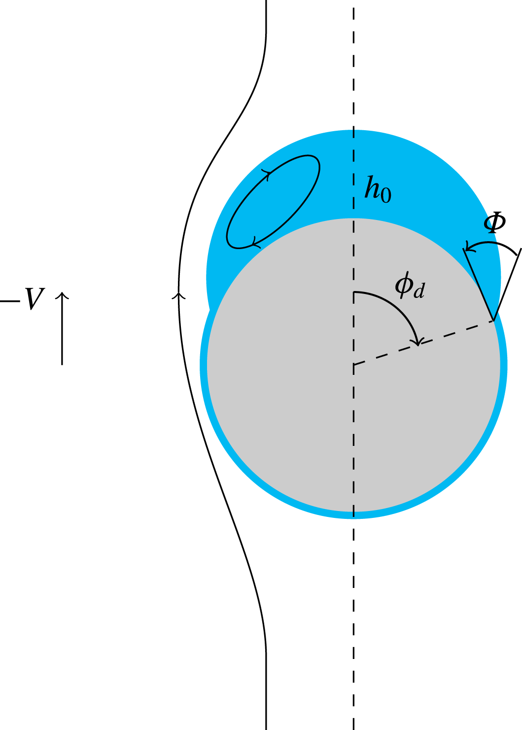
Figure 13. The geometry of the attached drop configuration in a reference frame translating with the sphere.
Within the drop, the fluid is set in motion by the stress distribution applied by the outer fluid on their common interface. The condition of zero flow rate across the drop at any angular position
 $\unicode[STIX]{x1D719}$
implies that this internal flow recirculates, reducing to a lubrication flow with a parabolic velocity profile in the limit of thin drops (
$\unicode[STIX]{x1D719}$
implies that this internal flow recirculates, reducing to a lubrication flow with a parabolic velocity profile in the limit of thin drops (
 $h_{0}/R\ll 1$
), and generating a traction at the drop/sphere interface that is half of that at the drop/outer-fluid interface (Johnson Reference Johnson1981). Hence, in that limit, the shear stress applied by the outer fluid results in an upward force on both interfaces, the sum of which, say
$h_{0}/R\ll 1$
), and generating a traction at the drop/sphere interface that is half of that at the drop/outer-fluid interface (Johnson Reference Johnson1981). Hence, in that limit, the shear stress applied by the outer fluid results in an upward force on both interfaces, the sum of which, say
 $F_{Ds}$
, is proportional to the area of the spherical cap covered by the drop, i.e. to
$F_{Ds}$
, is proportional to the area of the spherical cap covered by the drop, i.e. to
 $1-\cos \unicode[STIX]{x1D719}_{d}$
. Still in the limit
$1-\cos \unicode[STIX]{x1D719}_{d}$
. Still in the limit
 $h_{0}/R\ll 1$
, the pressure (more generally the normal stress) is almost constant across the drop at a given
$h_{0}/R\ll 1$
, the pressure (more generally the normal stress) is almost constant across the drop at a given
 $\unicode[STIX]{x1D719}$
, thus contributing to the net viscous force only through a small form drag, say
$\unicode[STIX]{x1D719}$
, thus contributing to the net viscous force only through a small form drag, say
 $F_{Dn}$
, proportional to the difference between the areas of the two interfaces, which itself is proportional to
$F_{Dn}$
, proportional to the difference between the areas of the two interfaces, which itself is proportional to
 $(1-\cos \unicode[STIX]{x1D719}_{d})h_{0}/R$
, i.e. to the drop volume. The total drag acting on the drop,
$(1-\cos \unicode[STIX]{x1D719}_{d})h_{0}/R$
, i.e. to the drop volume. The total drag acting on the drop,
 $F_{Dd}=F_{Ds}+F_{Dn}$
, may be formally written as
$F_{Dd}=F_{Ds}+F_{Dn}$
, may be formally written as
 $F_{Dd}=-6\unicode[STIX]{x03C0}\unicode[STIX]{x1D707}_{2}K_{d}RV$
, with
$F_{Dd}=-6\unicode[STIX]{x03C0}\unicode[STIX]{x1D707}_{2}K_{d}RV$
, with
 $K_{d}$
depending on both the viscosity ratio and the drop geometry.
$K_{d}$
depending on both the viscosity ratio and the drop geometry.
Collecting all contributions finally yields the vertical force balance on the drop in the form
 $$\begin{eqnarray}-2\unicode[STIX]{x03C0}R\unicode[STIX]{x1D6FE}\text{sin}\unicode[STIX]{x1D719}_{d}\left\{\sin (\unicode[STIX]{x1D719}_{d}+\unicode[STIX]{x1D6F7})-\frac{R}{R_{0}}\sin \unicode[STIX]{x1D719}_{d}\right\}+(\unicode[STIX]{x1D70C}_{2}-\unicode[STIX]{x1D70C}_{1})({\mathcal{V}}_{d}-{\mathcal{V}}_{0})g-6\unicode[STIX]{x03C0}\unicode[STIX]{x1D707}_{2}K_{d}RV=0.\end{eqnarray}$$
Condition (5.1) governs the settling velocity of the compound body, while (5.2) may be thought of as a global constraint relating the geometrical parameters of the drop, namely
 $\unicode[STIX]{x1D719}_{d}$
,
$\unicode[STIX]{x1D719}_{d}$
,
 $\unicode[STIX]{x1D6F7}$
,
$\unicode[STIX]{x1D6F7}$
,
 $R_{0}$
,
$R_{0}$
,
 $h_{0}$
and
$h_{0}$
and
 ${\mathcal{V}}_{d}$
. Injecting the solution of (5.1) into (5.2) yields
${\mathcal{V}}_{d}$
. Injecting the solution of (5.1) into (5.2) yields
 $$\begin{eqnarray}\frac{3}{2Bo}\sin ^{2}\unicode[STIX]{x1D719}_{d}\left(\frac{\sin (\unicode[STIX]{x1D719}_{d}+\unicode[STIX]{x1D6F7})}{\sin \unicode[STIX]{x1D719}_{d}}-\frac{R}{R_{0}}\right)+{\mathcal{V}}_{0}^{\ast }-{\mathcal{V}}_{d}^{\ast }-\left(\frac{\unicode[STIX]{x1D701}_{p}}{\unicode[STIX]{x1D701}}-1-{\mathcal{V}}_{d}^{\ast }\right)\frac{K_{d}}{1+K}=0,\end{eqnarray}$$
where
 ${\mathcal{V}}_{d}^{\ast }$
and
${\mathcal{V}}_{d}^{\ast }$
and
 ${\mathcal{V}}_{0}^{\ast }$
stand for
${\mathcal{V}}_{0}^{\ast }$
stand for
 ${\mathcal{V}}_{d}^{\ast }/{\mathcal{V}}$
and
${\mathcal{V}}_{d}^{\ast }/{\mathcal{V}}$
and
 ${\mathcal{V}}_{0}/{\mathcal{V}}$
respectively. When the sphere is at rest, the last term becomes irrelevant and (5.3) is then simply an integral constraint resulting from the Young–Laplace problem that governs the classical pendant drop configuration. In contrast, when the sphere moves with respect to the fluid, the drop volume is influenced by the last term on the left-hand side, and hence by the sphere-to-fluid density contrast through the factor
${\mathcal{V}}_{0}/{\mathcal{V}}$
respectively. When the sphere is at rest, the last term becomes irrelevant and (5.3) is then simply an integral constraint resulting from the Young–Laplace problem that governs the classical pendant drop configuration. In contrast, when the sphere moves with respect to the fluid, the drop volume is influenced by the last term on the left-hand side, and hence by the sphere-to-fluid density contrast through the factor
 $\unicode[STIX]{x1D701}_{p}/\unicode[STIX]{x1D701}-1=(\unicode[STIX]{x1D70C}_{p}-\unicode[STIX]{x1D70C}_{2})/(\unicode[STIX]{x1D70C}_{2}-\unicode[STIX]{x1D70C}_{1})$
. With
$\unicode[STIX]{x1D701}_{p}/\unicode[STIX]{x1D701}-1=(\unicode[STIX]{x1D70C}_{p}-\unicode[STIX]{x1D70C}_{2})/(\unicode[STIX]{x1D70C}_{2}-\unicode[STIX]{x1D70C}_{1})$
. With
 $K_{d}>0$
, this term tends to make the drop volume decrease compared with the static situation.
$K_{d}>0$
, this term tends to make the drop volume decrease compared with the static situation.
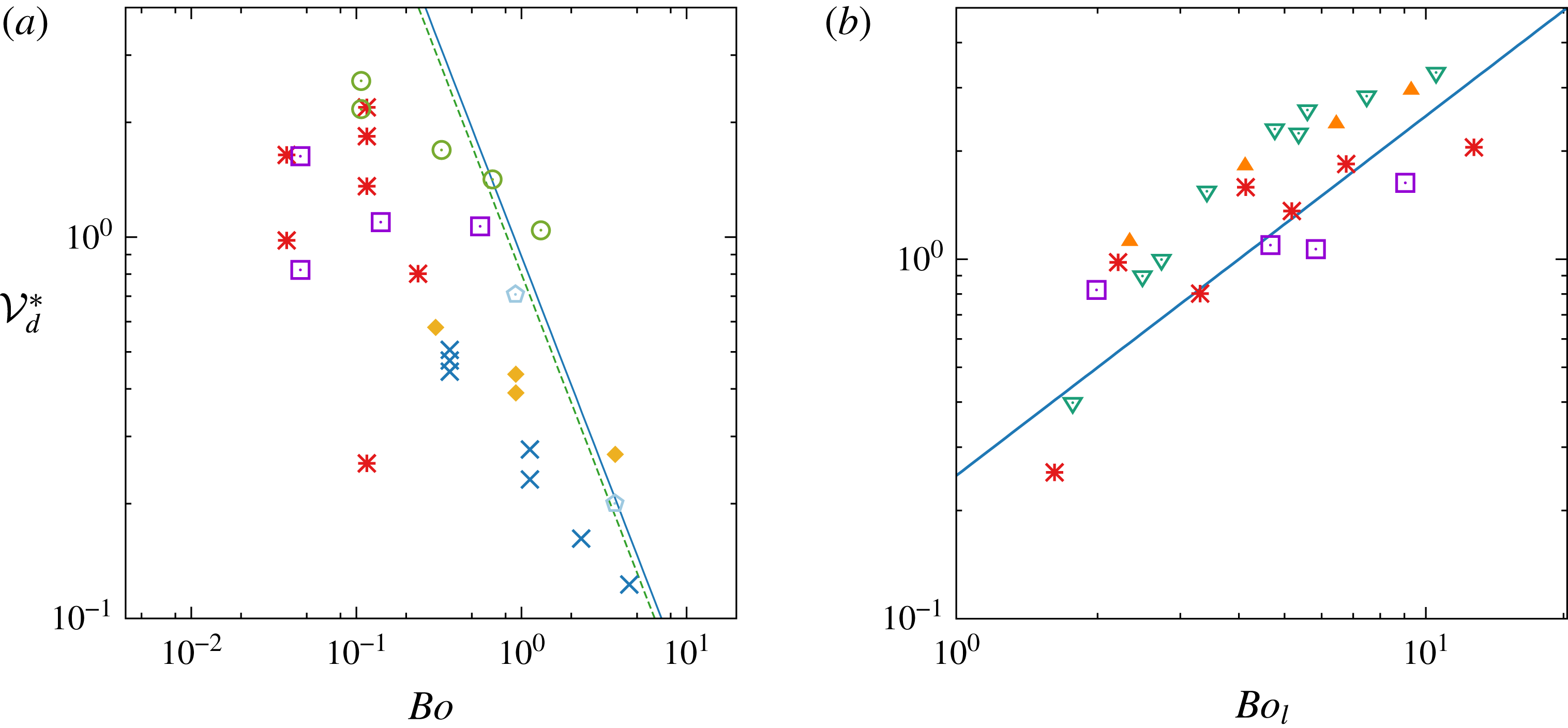
Figure 14. The volume of attached drops under various experimental conditions: (a)
 ${\mathcal{V}}_{d}^{\ast }$
versus
${\mathcal{V}}_{d}^{\ast }$
versus
 $Bo$
for various spheres in
$Bo$
for various spheres in
 $\times$
, V5/water–glycerin (
$\times$
, V5/water–glycerin (
 $\unicode[STIX]{x1D701}=0.32$
,
$\unicode[STIX]{x1D701}=0.32$
,
 $\unicode[STIX]{x1D706}=18.3$
); ♦, V50/water–glycerin (
$\unicode[STIX]{x1D706}=18.3$
); ♦, V50/water–glycerin (
 $\unicode[STIX]{x1D701}=0.26,\unicode[STIX]{x1D706}=1.7$
);
$\unicode[STIX]{x1D701}=0.26,\unicode[STIX]{x1D706}=1.7$
);
 $\unicode[STIX]{x2B20}$
, V500/water–glycerin (
$\unicode[STIX]{x2B20}$
, V500/water–glycerin (
 $\unicode[STIX]{x1D701}=0.24$
,
$\unicode[STIX]{x1D701}=0.24$
,
 $\unicode[STIX]{x1D706}=0.17$
);
$\unicode[STIX]{x1D706}=0.17$
);
 $\odot$
, V5/water (
$\odot$
, V5/water (
 $\unicode[STIX]{x1D701}\approx 0.09,\unicode[STIX]{x1D706}=0.21$
); ▫, V50/water (
$\unicode[STIX]{x1D701}\approx 0.09,\unicode[STIX]{x1D706}=0.21$
); ▫, V50/water (
 $\unicode[STIX]{x1D701}\approx 0.04,\unicode[STIX]{x1D706}=1.9\times 10^{-2}$
); *, V500/water (
$\unicode[STIX]{x1D701}\approx 0.04,\unicode[STIX]{x1D706}=1.9\times 10^{-2}$
); *, V500/water (
 $\unicode[STIX]{x1D701}\approx 0.03,\unicode[STIX]{x1D706}=1.9\times 10^{-3}$
); solid and dashed lines, empirical fit for the pendant drop configuration,
$\unicode[STIX]{x1D701}\approx 0.03,\unicode[STIX]{x1D706}=1.9\times 10^{-3}$
); solid and dashed lines, empirical fit for the pendant drop configuration,
 ${\mathcal{V}}_{d}^{\ast }=0.89(1-0.37\unicode[STIX]{x1D6F7}^{2})Bo^{-1.12}$
for
${\mathcal{V}}_{d}^{\ast }=0.89(1-0.37\unicode[STIX]{x1D6F7}^{2})Bo^{-1.12}$
for
 $\unicode[STIX]{x1D6F7}=0$
and
$\unicode[STIX]{x1D6F7}=0$
and
 $\unicode[STIX]{x03C0}/6$
respectively; (b)
$\unicode[STIX]{x03C0}/6$
respectively; (b)
 ${\mathcal{V}}_{d}^{\ast }$
versus
${\mathcal{V}}_{d}^{\ast }$
versus
 $Bo_{l}$
for various spheres in ▫, V50/water; *, V500/water; solid line, guide-to-the-eye line with a
$Bo_{l}$
for various spheres in ▫, V50/water; *, V500/water; solid line, guide-to-the-eye line with a
 $+1$
slope. Panel (b) also shows data from Pitois, Moucheront & Weill (Reference Pitois, Moucheront and Weill1999) obtained in a PDMS oil/water system (
$+1$
slope. Panel (b) also shows data from Pitois, Moucheront & Weill (Reference Pitois, Moucheront and Weill1999) obtained in a PDMS oil/water system (
 $\unicode[STIX]{x1D701}=2.9\times 10^{-2}$
,
$\unicode[STIX]{x1D701}=2.9\times 10^{-2}$
,
 $\unicode[STIX]{x1D706}=1.\times 10^{-4}$
); ▿, steel spheres with various radii; ▴, glass spheres with various radii.
$\unicode[STIX]{x1D706}=1.\times 10^{-4}$
); ▿, steel spheres with various radii; ▴, glass spheres with various radii.
5.2 Experimental results and scaling laws for the drop volume
We determined the drop volumes by post-processing raw images using a contour detection technique and assuming axisymmetric shapes. To compare the corresponding results with drop volumes found with a sphere at rest, we examined the numerical predictions obtained by Shoukry et al. (Reference Shoukry, Hafez and Hartland1975) (for
 $\unicode[STIX]{x1D6F7}=0^{\circ }$
, up to
$\unicode[STIX]{x1D6F7}=0^{\circ }$
, up to
 $Bo=100$
) and Smith & Van de Den (Reference Smith and Van de Den1985) (for all
$Bo=100$
) and Smith & Van de Den (Reference Smith and Van de Den1985) (for all
 $\unicode[STIX]{x1D6F7}$
, up to
$\unicode[STIX]{x1D6F7}$
, up to
 $Bo=1$
). We found that these results are accurately fitted (at least up to
$Bo=1$
). We found that these results are accurately fitted (at least up to
 $\unicode[STIX]{x1D6F7}=30^{\circ }$
, the largest pseudo-contact angle observed in our experiments) by the empirical formula
$\unicode[STIX]{x1D6F7}=30^{\circ }$
, the largest pseudo-contact angle observed in our experiments) by the empirical formula
 ${\mathcal{V}}_{d}^{\ast }=0.89(1-0.37\unicode[STIX]{x1D6F7}^{2})Bo^{-1.12}$
. It should be noted that in this formula the Bond number has a slightly larger negative exponent than suggested by the explicit
${\mathcal{V}}_{d}^{\ast }=0.89(1-0.37\unicode[STIX]{x1D6F7}^{2})Bo^{-1.12}$
. It should be noted that in this formula the Bond number has a slightly larger negative exponent than suggested by the explicit
 $Bo^{-1}$
dependence in (5.3). This is because the drop geometry, i.e. the relation between
$Bo^{-1}$
dependence in (5.3). This is because the drop geometry, i.e. the relation between
 $h_{0}$
,
$h_{0}$
,
 $R_{0}$
and
$R_{0}$
and
 $\unicode[STIX]{x1D719}_{d}$
, also varies with
$\unicode[STIX]{x1D719}_{d}$
, also varies with
 $Bo$
.
$Bo$
.
Figure 14(a) displays the drop volumes determined from a number of experimental tests versus the Bond number, using log–log coordinates. Also drawn in the figure are two lines corresponding to the aforementioned fit for
 $\unicode[STIX]{x1D6F7}=0^{\circ }$
and
$\unicode[STIX]{x1D6F7}=0^{\circ }$
and
 $30^{\circ }$
respectively. First of all, it is clear from this figure that, apart from two exceptions, all measured volumes are smaller than those found in the static configuration. This confirms that the flow at the drop surface acts against capillary effects, reducing the size of drops that can remain attached to the sphere. This figure also reveals that data obtained in the V50/water and V500/water pairs of fluids with spheres of different densities and diameters do not exhibit any clear trend, implying that the Bond number is not a relevant scaling parameter under such conditions. To understand why, one has to notice that, among the pairs of fluids considered here, these are the two with the smallest density (and viscosity) contrasts. According to (5.3), the smaller
$30^{\circ }$
respectively. First of all, it is clear from this figure that, apart from two exceptions, all measured volumes are smaller than those found in the static configuration. This confirms that the flow at the drop surface acts against capillary effects, reducing the size of drops that can remain attached to the sphere. This figure also reveals that data obtained in the V50/water and V500/water pairs of fluids with spheres of different densities and diameters do not exhibit any clear trend, implying that the Bond number is not a relevant scaling parameter under such conditions. To understand why, one has to notice that, among the pairs of fluids considered here, these are the two with the smallest density (and viscosity) contrasts. According to (5.3), the smaller
 $\unicode[STIX]{x1D701}$
is, the larger the influence of the last term on the left-hand side, i.e. of the sphere motion, is on the drop volume. Hence, the corresponding problem has little in common with the static pendant drop configuration and there is no reason why volumes of drops attached to spheres with different
$\unicode[STIX]{x1D701}$
is, the larger the influence of the last term on the left-hand side, i.e. of the sphere motion, is on the drop volume. Hence, the corresponding problem has little in common with the static pendant drop configuration and there is no reason why volumes of drops attached to spheres with different
 $\unicode[STIX]{x1D701}_{p}$
values should exhibit any systematic variation with respect to
$\unicode[STIX]{x1D701}_{p}$
values should exhibit any systematic variation with respect to
 $Bo$
in that limit. Then, it appears relevant to consider (5.3) in the limit
$Bo$
in that limit. Then, it appears relevant to consider (5.3) in the limit
 $\unicode[STIX]{x1D701}\rightarrow 0$
. As terms due to buoyancy effects then become negligibly small, (5.3) may be simplified to
$\unicode[STIX]{x1D701}\rightarrow 0$
. As terms due to buoyancy effects then become negligibly small, (5.3) may be simplified to
 $$\begin{eqnarray}\frac{3}{2Bo_{l}}\sin ^{2}\unicode[STIX]{x1D719}_{d}\left(\frac{\sin (\unicode[STIX]{x1D719}_{d}+\unicode[STIX]{x1D6F7})}{\sin \unicode[STIX]{x1D719}_{d}}-\frac{R}{R_{0}}\right)\approx \frac{K_{d}}{1+K},\end{eqnarray}$$
with
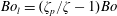 $Bo_{l}=(\unicode[STIX]{x1D701}_{p}/\unicode[STIX]{x1D701}-1)Bo$
as defined earlier. Condition (5.4) suggests that drop volumes primarily depend on
$Bo_{l}=(\unicode[STIX]{x1D701}_{p}/\unicode[STIX]{x1D701}-1)Bo$
as defined earlier. Condition (5.4) suggests that drop volumes primarily depend on
 $Bo_{l}$
when
$Bo_{l}$
when
 $\unicode[STIX]{x1D701}$
is small. Figure 14(b) confirms this conjecture for the aforementioned two series which have
$\unicode[STIX]{x1D701}$
is small. Figure 14(b) confirms this conjecture for the aforementioned two series which have
 $\unicode[STIX]{x1D701}=0.04$
and
$\unicode[STIX]{x1D701}=0.04$
and
 $0.03$
respectively. Although the plot contains a non-negligible scatter, drop volumes are seen to increase consistently with
$0.03$
respectively. Although the plot contains a non-negligible scatter, drop volumes are seen to increase consistently with
 $Bo_{l}$
, mostly in a linear manner. The figure also displays data from Pitois et al. (Reference Pitois, Moucheront and Weill1999), who, under quite similar conditions, concluded that
$Bo_{l}$
, mostly in a linear manner. The figure also displays data from Pitois et al. (Reference Pitois, Moucheront and Weill1999), who, under quite similar conditions, concluded that
 ${\mathcal{V}}_{d}^{\ast }$
varies approximately as the logarithm of
${\mathcal{V}}_{d}^{\ast }$
varies approximately as the logarithm of
 $Bo_{l}$
.
$Bo_{l}$
.
The other three series in figure 14(a) behave more consistently, all of them exhibiting a clear decrease of
 ${\mathcal{V}}_{d}^{\ast }$
as
${\mathcal{V}}_{d}^{\ast }$
as
 $Bo$
increases. However, the average slope in each series is always less than
$Bo$
increases. However, the average slope in each series is always less than
 $-0.8$
, and hence significantly smaller than the one observed in the pendant drop configuration. Although materials are not specified in the figure, the sphere density increases from right to left in the two series involving the water–glycerin mixture, i.e. those with the largest
$-0.8$
, and hence significantly smaller than the one observed in the pendant drop configuration. Although materials are not specified in the figure, the sphere density increases from right to left in the two series involving the water–glycerin mixture, i.e. those with the largest
 $\unicode[STIX]{x1D701}$
(since small ‘light’ spheres float, only small ‘heavy’ spheres are capable of entraining a drop). The role of this parameter may be readily appreciated in the case of the V5/water–glycerin pair, for which
$\unicode[STIX]{x1D701}$
(since small ‘light’ spheres float, only small ‘heavy’ spheres are capable of entraining a drop). The role of this parameter may be readily appreciated in the case of the V5/water–glycerin pair, for which
 $\unicode[STIX]{x1D706}=18.3$
. With this large
$\unicode[STIX]{x1D706}=18.3$
. With this large
 $\unicode[STIX]{x1D706}$
, the shear stress at the drop surface is almost zero, making the drag force on the drop,
$\unicode[STIX]{x1D706}$
, the shear stress at the drop surface is almost zero, making the drag force on the drop,
 $F_{Dd}$
, reduce essentially to the contribution of the normal stress,
$F_{Dd}$
, reduce essentially to the contribution of the normal stress,
 $F_{Dn}$
. As we showed above, in the limit
$F_{Dn}$
. As we showed above, in the limit
 $h_{0}/R\ll 1$
, the latter is proportional to the drop volume. Hence, in (5.3),
$h_{0}/R\ll 1$
, the latter is proportional to the drop volume. Hence, in (5.3),
 $K_{d}\propto {\mathcal{V}}_{d}^{\ast }$
, so that the term
$K_{d}\propto {\mathcal{V}}_{d}^{\ast }$
, so that the term
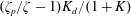 $(\unicode[STIX]{x1D701}_{p}/\unicode[STIX]{x1D701}-1)K_{d}/(1+K)$
merely acts as an additional buoyancy force, thus reducing the drop volume for a given
$(\unicode[STIX]{x1D701}_{p}/\unicode[STIX]{x1D701}-1)K_{d}/(1+K)$
merely acts as an additional buoyancy force, thus reducing the drop volume for a given
 $Bo$
(in the limit
$Bo$
(in the limit
 ${\mathcal{V}}_{d}^{\ast }\ll 1$
,
${\mathcal{V}}_{d}^{\ast }\ll 1$
,
 $K\approx -1/3$
because the presence of the low-viscosity film and drop makes the compound body behave nearly as a bubble, and the drag force on a spherical bubble is
$K\approx -1/3$
because the presence of the low-viscosity film and drop makes the compound body behave nearly as a bubble, and the drag force on a spherical bubble is
 $2/3$
of that on a rigid sphere). A comparison of corresponding data in figure 14(a) with the fit determined for static pendant drops reveals how dramatic the reduction of
$2/3$
of that on a rigid sphere). A comparison of corresponding data in figure 14(a) with the fit determined for static pendant drops reveals how dramatic the reduction of
 ${\mathcal{V}}_{d}^{\ast }$
due to the solid-to-fluid density contrast is: while the drop volume measured for the largest and lightest sphere (
${\mathcal{V}}_{d}^{\ast }$
due to the solid-to-fluid density contrast is: while the drop volume measured for the largest and lightest sphere (
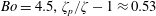 $Bo=4.5,\unicode[STIX]{x1D701}_{p}/\unicode[STIX]{x1D701}-1\approx 0.53$
) is close to that predicted by the fit for this specific
$Bo=4.5,\unicode[STIX]{x1D701}_{p}/\unicode[STIX]{x1D701}-1\approx 0.53$
) is close to that predicted by the fit for this specific
 $Bo$
, it is roughly four times less for the smallest and heaviest sphere (
$Bo$
, it is roughly four times less for the smallest and heaviest sphere (
 $Bo=0.37,\unicode[STIX]{x1D701}_{p}/\unicode[STIX]{x1D701}-1\approx 9.1$
). Hence, in figure 14(a), the reduction of the drop volume through the influence of the solid-to-fluid density contrast is larger on the left part of the series (small
$Bo=0.37,\unicode[STIX]{x1D701}_{p}/\unicode[STIX]{x1D701}-1\approx 9.1$
). Hence, in figure 14(a), the reduction of the drop volume through the influence of the solid-to-fluid density contrast is larger on the left part of the series (small
 $Bo$
, large
$Bo$
, large
 $\unicode[STIX]{x1D701}_{p}/\unicode[STIX]{x1D701}$
) than on the right part (large
$\unicode[STIX]{x1D701}_{p}/\unicode[STIX]{x1D701}$
) than on the right part (large
 $Bo$
, small
$Bo$
, small
 $\unicode[STIX]{x1D701}_{p}/\unicode[STIX]{x1D701}$
), resulting in variations with the Bond number looking weaker than those of static pendant drops. This implies that a proper representation of the
$\unicode[STIX]{x1D701}_{p}/\unicode[STIX]{x1D701}$
), resulting in variations with the Bond number looking weaker than those of static pendant drops. This implies that a proper representation of the
 ${\mathcal{V}}_{d}^{\ast }$
variations should make use of the three-dimensional space
${\mathcal{V}}_{d}^{\ast }$
variations should make use of the three-dimensional space
 $({\mathcal{V}}_{d}^{\ast },Bo,\unicode[STIX]{x1D701}_{p}/\unicode[STIX]{x1D701})$
, the representation in the
$({\mathcal{V}}_{d}^{\ast },Bo,\unicode[STIX]{x1D701}_{p}/\unicode[STIX]{x1D701})$
, the representation in the
 $({\mathcal{V}}_{d}^{\ast },Bo)$
plane mixing two distinct effects. However, there is a priori no reason why the static exponent
$({\mathcal{V}}_{d}^{\ast },Bo)$
plane mixing two distinct effects. However, there is a priori no reason why the static exponent
 $-1.12$
should be recovered for a given
$-1.12$
should be recovered for a given
 $\unicode[STIX]{x1D701}_{p}/\unicode[STIX]{x1D701}$
in that three-dimensional representation because the influence of the outer flow certainly alters the drop geometry, i.e. the relation between
$\unicode[STIX]{x1D701}_{p}/\unicode[STIX]{x1D701}$
in that three-dimensional representation because the influence of the outer flow certainly alters the drop geometry, i.e. the relation between
 ${\mathcal{V}}_{d}$
,
${\mathcal{V}}_{d}$
,
 $h_{0},R_{0}$
and
$h_{0},R_{0}$
and
 $\unicode[STIX]{x1D719}_{d}$
, as the sequence in figure 11 suggests. Unfortunately, we have no means to evaluate this possible alteration at the present stage, as this would require significantly more data with each material in each pair of fluids.
$\unicode[STIX]{x1D719}_{d}$
, as the sequence in figure 11 suggests. Unfortunately, we have no means to evaluate this possible alteration at the present stage, as this would require significantly more data with each material in each pair of fluids.
The situation described above for fluid pairs having significant density contrasts indicates that none of the terms on the left-hand side of (5.3) are really negligible under such conditions. This state of affairs, combined with the subtle interdependence of the geometric parameters,
 $R_{0}$
,
$R_{0}$
,
 $h_{0}$
and
$h_{0}$
and
 $\unicode[STIX]{x1D719}_{d}$
, makes the prediction of exact scaling laws for the drop volume based on simple models for the drag factors
$\unicode[STIX]{x1D719}_{d}$
, makes the prediction of exact scaling laws for the drop volume based on simple models for the drag factors
 $K_{d}$
and
$K_{d}$
and
 $K$
presumably out of reach. The situation simplifies in the limit
$K$
presumably out of reach. The situation simplifies in the limit
 $\unicode[STIX]{x1D701}\rightarrow 0$
, where the linear increase of
$\unicode[STIX]{x1D701}\rightarrow 0$
, where the linear increase of
 ${\mathcal{V}}_{d}^{\ast }$
with
${\mathcal{V}}_{d}^{\ast }$
with
 $Bo_{l}$
can be readily inferred from (5.4). For this, one first has to notice that the corresponding drops have a quite flat top (see panels (d–f) in figure 12). Thus, the radius of curvature
$Bo_{l}$
can be readily inferred from (5.4). For this, one first has to notice that the corresponding drops have a quite flat top (see panels (d–f) in figure 12). Thus, the radius of curvature
 $R_{0}$
is larger than
$R_{0}$
is larger than
 $R$
, and the positive difference
$R$
, and the positive difference
 $1-R/R_{0}$
increases with
$1-R/R_{0}$
increases with
 $h_{0}$
, and hence with
$h_{0}$
, and hence with
 ${\mathcal{V}}_{d}^{\ast }$
(one would have
${\mathcal{V}}_{d}^{\ast }$
(one would have
 $1-R/R_{0}\approx h_{0}/R$
for a thin spherical drop). For small
$1-R/R_{0}\approx h_{0}/R$
for a thin spherical drop). For small
 $\unicode[STIX]{x1D6F7}$
and
$\unicode[STIX]{x1D6F7}$
and
 $\unicode[STIX]{x1D719}_{d}\approx \unicode[STIX]{x03C0}/2$
(which is qualitatively consistent with the aforementioned panels), the left-hand side of (5.4) is then virtually directly proportional to
$\unicode[STIX]{x1D719}_{d}\approx \unicode[STIX]{x03C0}/2$
(which is qualitatively consistent with the aforementioned panels), the left-hand side of (5.4) is then virtually directly proportional to
 ${\mathcal{V}}_{d}^{\ast }/Bo_{l}$
. In the present experiments, pairs of fluids with small
${\mathcal{V}}_{d}^{\ast }/Bo_{l}$
. In the present experiments, pairs of fluids with small
 $\unicode[STIX]{x1D701}$
also have small
$\unicode[STIX]{x1D701}$
also have small
 $\unicode[STIX]{x1D706}$
, so that the outer fluid almost obeys a no-slip condition at the drop surface. In the limit
$\unicode[STIX]{x1D706}$
, so that the outer fluid almost obeys a no-slip condition at the drop surface. In the limit
 $h_{0}/R\ll 1$
, the drag force on the drop,
$h_{0}/R\ll 1$
, the drag force on the drop,
 $F_{Dd}$
, is then dominated by the shear-induced contribution,
$F_{Dd}$
, is then dominated by the shear-induced contribution,
 $F_{Ds}$
. As shown above, the latter is proportional to the area of the spherical cap covered by the drop, implying
$F_{Ds}$
. As shown above, the latter is proportional to the area of the spherical cap covered by the drop, implying
 $K_{d}\propto 1-\cos \unicode[STIX]{x1D719}_{d}$
. In the same limit,
$K_{d}\propto 1-\cos \unicode[STIX]{x1D719}_{d}$
. In the same limit,
 $1+K\rightarrow 1$
, because the compound body behaves essentially as a solid sphere, so that the right-hand side of (5.4),
$1+K\rightarrow 1$
, because the compound body behaves essentially as a solid sphere, so that the right-hand side of (5.4),
 $K_{d}/(1+K)$
, tends towards a non-zero value which only depends on the cap angle
$K_{d}/(1+K)$
, tends towards a non-zero value which only depends on the cap angle
 $\unicode[STIX]{x1D719}_{d}$
(note the difference with the case discussed above for
$\unicode[STIX]{x1D719}_{d}$
(note the difference with the case discussed above for
 $\unicode[STIX]{x1D706}\gg 1$
, where
$\unicode[STIX]{x1D706}\gg 1$
, where
 $K_{d}/(1+K)\propto {\mathcal{V}}_{d}^{\ast }$
). Balancing both sides of (5.4) then requires
$K_{d}/(1+K)\propto {\mathcal{V}}_{d}^{\ast }$
). Balancing both sides of (5.4) then requires
 ${\mathcal{V}}_{d}^{\ast }$
to increase linearly with
${\mathcal{V}}_{d}^{\ast }$
to increase linearly with
 $Bo_{l}$
.
$Bo_{l}$
.
Finally, it is important to keep in mind that in the present experiments, pairs of fluids with small
 $\unicode[STIX]{x1D701}$
also have small
$\unicode[STIX]{x1D701}$
also have small
 $\unicode[STIX]{x1D706}$
, while those with significant
$\unicode[STIX]{x1D706}$
, while those with significant
 $\unicode[STIX]{x1D701}$
have moderate-to-large
$\unicode[STIX]{x1D701}$
have moderate-to-large
 $\unicode[STIX]{x1D706}$
. Therefore, it is not clear how far the observed tendencies for
$\unicode[STIX]{x1D706}$
. Therefore, it is not clear how far the observed tendencies for
 ${\mathcal{V}}_{d}^{\ast }$
to decrease with increasing
${\mathcal{V}}_{d}^{\ast }$
to decrease with increasing
 $Bo$
for
$Bo$
for
 $\unicode[STIX]{x1D701}\gtrsim 0.1$
, and to increase with increasing
$\unicode[STIX]{x1D701}\gtrsim 0.1$
, and to increase with increasing
 $Bo_{l}$
for smaller
$Bo_{l}$
for smaller
 $\unicode[STIX]{x1D701}$
, are independent of
$\unicode[STIX]{x1D701}$
, are independent of
 $\unicode[STIX]{x1D706}$
. Additional experiments with selected fluid pairs having significant
$\unicode[STIX]{x1D706}$
. Additional experiments with selected fluid pairs having significant
 $\unicode[STIX]{x1D701}$
but small
$\unicode[STIX]{x1D701}$
but small
 $\unicode[STIX]{x1D706}$
and vice versa are desirable to complete this picture.
$\unicode[STIX]{x1D706}$
and vice versa are desirable to complete this picture.
6 Tail fragmentation
6.1 Observations and underlying mechanisms

Figure 15. Fragmentation in the tail past a 14 mm steel sphere in (a) the V5/water pair (configuration
 $18b$
;
$18b$
;
 $\unicode[STIX]{x1D706}=0.21,\unicode[STIX]{x1D701}=0.09,\unicode[STIX]{x1D701}_{p}=7.6,Ar=970,Bo=1.3$
), (b) the V50/water pair (configuration
$\unicode[STIX]{x1D706}=0.21,\unicode[STIX]{x1D701}=0.09,\unicode[STIX]{x1D701}_{p}=7.6,Ar=970,Bo=1.3$
), (b) the V50/water pair (configuration
 $27a$
;
$27a$
;
 $\unicode[STIX]{x1D706}=0.02,\unicode[STIX]{x1D701}=0.04,\unicode[STIX]{x1D701}_{p}=7.2,Ar=91,Bo=0.55$
) and (c) the V50/water pair with Triton X-100 (configuration
$\unicode[STIX]{x1D706}=0.02,\unicode[STIX]{x1D701}=0.04,\unicode[STIX]{x1D701}_{p}=7.2,Ar=91,Bo=0.55$
) and (c) the V50/water pair with Triton X-100 (configuration
 $27a_{s}$
; same parameters as in (b) except that here
$27a_{s}$
; same parameters as in (b) except that here
 $Bo=5.1$
).
$Bo=5.1$
).
Figure 15 displays three sequences showing the early stages of the fragmentation process in the tail past a
 $14~\text{mm}$
steel sphere falling in water (these correspond to configurations 18b, 27a and 27
$14~\text{mm}$
steel sphere falling in water (these correspond to configurations 18b, 27a and 27
 $a_{s}$
in § 3.2 respectively). All three cases therefore share the same value of
$a_{s}$
in § 3.2 respectively). All three cases therefore share the same value of
 $Ar_{l}$
, namely
$Ar_{l}$
, namely
 $Ar_{l}\approx 4.8\times 10^{3}$
. They essentially differ by the viscosity of the upper fluid, which is 10 times larger in (b) and (c) than in (a), and the presence of Triton X-100 in (c), which makes the Bond number
$Ar_{l}\approx 4.8\times 10^{3}$
. They essentially differ by the viscosity of the upper fluid, which is 10 times larger in (b) and (c) than in (a), and the presence of Triton X-100 in (c), which makes the Bond number
 $Bo_{l}$
rise up to
$Bo_{l}$
rise up to
 $Bo_{l}=1.01\times 10^{3}$
, whereas
$Bo_{l}=1.01\times 10^{3}$
, whereas
 $Bo_{l}=115$
and
$Bo_{l}=115$
and
 $111$
in (a) and (b) respectively. Videos displaying the corresponding three sequences are available online in the supplementary material. No fragmentation takes place in the wake of the same steel sphere with the V500/water pair of fluids (configuration 27b), although
$111$
in (a) and (b) respectively. Videos displaying the corresponding three sequences are available online in the supplementary material. No fragmentation takes place in the wake of the same steel sphere with the V500/water pair of fluids (configuration 27b), although
 $Ar_{l}$
is unchanged and the Bond number is similar to those of cases (a) and (b) (
$Ar_{l}$
is unchanged and the Bond number is similar to those of cases (a) and (b) (
 $Bo_{l}=123$
). This is a clear indication that, for a given kinetic energy of the sphere and given levels of capillary and viscous stresses exerted by the outer fluid, fragmentation can only occur if the viscosity of the inner fluid is low enough to allow large deformation of fluid parcels. The development of the breakup process in cases (a) and (b), as well as the absence of breakup in the aforementioned case, can be appreciated in more detail in the videos available as supplementary material https://doi.org/10.1017/jfm.2017.747.
$Bo_{l}=123$
). This is a clear indication that, for a given kinetic energy of the sphere and given levels of capillary and viscous stresses exerted by the outer fluid, fragmentation can only occur if the viscosity of the inner fluid is low enough to allow large deformation of fluid parcels. The development of the breakup process in cases (a) and (b), as well as the absence of breakup in the aforementioned case, can be appreciated in more detail in the videos available as supplementary material https://doi.org/10.1017/jfm.2017.747.
In all three sequences of figure 15, longitudinal ligaments, which are usual precursors of fragmentation in shear flows (Villermaux Reference Villermaux2007), develop at the back of the sphere, invading the entire tail progressively. However, these ligaments start to form immediately after the sphere crosses the interface in the case of the least viscous oil, whereas the tail remains axisymmetric and exhibits prominent corollas during a significant period of time in (b) and (c). The reason for this difference must be sought in the upper fluid: as the corresponding
 $Ar$
is of
$Ar$
is of
 $O(10^{3})$
with the least viscous oil, the flow in the wake becomes unstable well before the sphere reaches the interface, quickly generating three-dimensional vortex structures and small but non-zero horizontal displacements and rotations of the sphere. This may be appreciated in the top part of the sequence (a), where the funnel-shaped entrained column just below the interface is seen to be significantly non-vertical. In contrast, in (b) and (c),
$O(10^{3})$
with the least viscous oil, the flow in the wake becomes unstable well before the sphere reaches the interface, quickly generating three-dimensional vortex structures and small but non-zero horizontal displacements and rotations of the sphere. This may be appreciated in the top part of the sequence (a), where the funnel-shaped entrained column just below the interface is seen to be significantly non-vertical. In contrast, in (b) and (c),
 $Ar$
is of
$Ar$
is of
 $O(10^{2})$
, so that the flow past the sphere is still almost axisymmetric when it reaches the interface (see § 3.3). Wake instability, and hence three-dimensionality, then takes a finite time to develop while the sphere settles in the lower fluid, and it is only after this time lapse that ligaments start to form.
$O(10^{2})$
, so that the flow past the sphere is still almost axisymmetric when it reaches the interface (see § 3.3). Wake instability, and hence three-dimensionality, then takes a finite time to develop while the sphere settles in the lower fluid, and it is only after this time lapse that ligaments start to form.
In the case of liquid jets sheared by a gas stream, the Rayleigh–Taylor instability has been shown to be key in ligament formation (Marmottant & Villermaux Reference Marmottant and Villermaux2004). Here, the capillary length
 $l_{c}$
in (b) is approximately
$l_{c}$
in (b) is approximately
 $9.3~\text{mm}$
, i.e.
$9.3~\text{mm}$
, i.e.
 $1.3R$
, due to the weak density contrast between the two fluids. As the radius of the entrained column is of
$1.3R$
, due to the weak density contrast between the two fluids. As the radius of the entrained column is of
 $O(R)$
, the largest wavelength that can form in the azimuthal direction corresponds to a wavenumber
$O(R)$
, the largest wavelength that can form in the azimuthal direction corresponds to a wavenumber
 $k_{m}\approx R^{-1}$
. Thus,
$k_{m}\approx R^{-1}$
. Thus,
 $k_{m}\approx 1.3l_{c}^{-1}$
, which is beyond the cutoff wavenumber
$k_{m}\approx 1.3l_{c}^{-1}$
, which is beyond the cutoff wavenumber
 $k_{co}=l_{c}^{-1}$
of the Rayleigh–Taylor instability (Chandrasekar Reference Chandrasekar1961). Thus, this mechanism cannot be responsible for the formation of the ligaments in that case. Due to the presence of Triton X-100,
$k_{co}=l_{c}^{-1}$
of the Rayleigh–Taylor instability (Chandrasekar Reference Chandrasekar1961). Thus, this mechanism cannot be responsible for the formation of the ligaments in that case. Due to the presence of Triton X-100,
 $l_{c}$
is decreased to
$l_{c}$
is decreased to
 ${\approx}\!3~\text{mm}$
in (c), i.e.
${\approx}\!3~\text{mm}$
in (c), i.e.
 $k_{m}l_{c}\approx 0.45$
, which makes the largest structures in the tail potentially unstable through the Rayleigh–Taylor mechanism. Nevertheless, most of the three-dimensional structures seen to develop in (c) are of much smaller size, again making this mechanism unable to explain their formation. Wake instability, which eventually results in a turbulent wake, is thus responsible for the generation of three-dimensional structures, and hence of longitudinal ligaments, in all three sequences of figure 15.
$k_{m}l_{c}\approx 0.45$
, which makes the largest structures in the tail potentially unstable through the Rayleigh–Taylor mechanism. Nevertheless, most of the three-dimensional structures seen to develop in (c) are of much smaller size, again making this mechanism unable to explain their formation. Wake instability, which eventually results in a turbulent wake, is thus responsible for the generation of three-dimensional structures, and hence of longitudinal ligaments, in all three sequences of figure 15.

Figure 16. The evolution of the fragmented wake of a 14 mm steel sphere in the V5/water pair (a) and the V50/water pair (b).
Visual inspection of these three sequences also makes it clear that the average size of the ligaments and large droplets that form in the wake is smaller in (a) than in (b). This may be even better appreciated from figure 16, which provides a closer view of the wake evolution for these two cases. In figure 16(b), one notices the fairly cylindrical shape of the ligaments, at the tip of which droplets are seen to form; the ligaments clearly exhibit more wrinkled shapes in figure 16(a). We confirmed the difference in the average size of the large droplets formed during wake fragmentation by processing images taken at later time in the three sequences (with the sphere standing approximately
 $25R$
below the initial interface). More precisely, we identified a group of 40–80 nearly circular drops in each series of images using a contour detection routine, and employed Hough transform to determine the circle that best fitted each of them. We repeated the analysis with three separate runs in each series of experiments, to reduce statistical uncertainty. Unfortunately, the detection technique could not properly identify fragments smaller than 3–5 pixels, limiting our analysis to droplets larger than
$25R$
below the initial interface). More precisely, we identified a group of 40–80 nearly circular drops in each series of images using a contour detection routine, and employed Hough transform to determine the circle that best fitted each of them. We repeated the analysis with three separate runs in each series of experiments, to reduce statistical uncertainty. Unfortunately, the detection technique could not properly identify fragments smaller than 3–5 pixels, limiting our analysis to droplets larger than
 $0.30\pm 0.08$
mm in diameter with the present optical device. This restriction and the too limited available samples of drops prevented us from determining other statistical properties of the size distribution, especially its probability density function. For the population of ‘large’ droplets we considered, the above procedure yielded mean radii of
$0.30\pm 0.08$
mm in diameter with the present optical device. This restriction and the too limited available samples of drops prevented us from determining other statistical properties of the size distribution, especially its probability density function. For the population of ‘large’ droplets we considered, the above procedure yielded mean radii of
 $0.625$
,
$0.625$
,
 $0.84$
and
$0.84$
and
 $0.78~\text{mm}$
in (a), (b) and (c) respectively, with a 1 pixel uncertainty amounting to
$0.78~\text{mm}$
in (a), (b) and (c) respectively, with a 1 pixel uncertainty amounting to
 $\pm 0.04~\text{mm}$
. Since the pairs of fluids in series (a) and (b) have almost identical interfacial tensions, the noticeable difference in the corresponding two mean radii underlines the strong influence of the viscosity of the upper fluid (i.e. the one that forms the tail) on the outcome of the fragmentation process. In contrast, the fairly small difference in the mean radii found for series (b) and (c), which have identical viscosities but interfacial tensions differing by one order of magnitude, is quite remarkable.
$\pm 0.04~\text{mm}$
. Since the pairs of fluids in series (a) and (b) have almost identical interfacial tensions, the noticeable difference in the corresponding two mean radii underlines the strong influence of the viscosity of the upper fluid (i.e. the one that forms the tail) on the outcome of the fragmentation process. In contrast, the fairly small difference in the mean radii found for series (b) and (c), which have identical viscosities but interfacial tensions differing by one order of magnitude, is quite remarkable.
6.2 A phenomenological statistical model
The influence of surface tension and viscosity on the statistical characteristics of drop and bubble distributions resulting from turbulent breakup is well known, and considerable effort has been invested to quantify it in various types of flows, especially in the context of chemical engineering applications (see, e.g., Coulaloglou & Tavlarides (Reference Coulaloglou and Tavlarides1977), Tsouris & Tavlarides (Reference Tsouris and Tavlarides1994), Luo & Svendsen (Reference Luo and Svendsen1996) and references therein). However, the present situation, in which the wake is in a transitional state, makes it useful to revisit the underlying stress balances in the more general context of inertia-dominated carrying flows in which the efficient spatial scales comparable with the droplet size do not necessarily obey the usual scaling laws of high-Reynolds-number turbulence.
If
 $\unicode[STIX]{x1D706}$
is large, making the effects of the internal viscosity negligible, breakup is expected to occur as soon as the pressure difference
$\unicode[STIX]{x1D706}$
is large, making the effects of the internal viscosity negligible, breakup is expected to occur as soon as the pressure difference
 $\unicode[STIX]{x0394}p(\mathfrak{r})$
along the surface of a ligament with radius
$\unicode[STIX]{x0394}p(\mathfrak{r})$
along the surface of a ligament with radius
 $\mathfrak{r}$
exceeds the restoring capillary pressure, which is of
$\mathfrak{r}$
exceeds the restoring capillary pressure, which is of
 $O(\unicode[STIX]{x1D6FE}/\mathfrak{r})$
. Assuming that the motion in the outer fluid is dominated by inertia, one has
$O(\unicode[STIX]{x1D6FE}/\mathfrak{r})$
. Assuming that the motion in the outer fluid is dominated by inertia, one has
 $\unicode[STIX]{x0394}p(\mathfrak{r})\propto \unicode[STIX]{x1D70C}_{2}(\unicode[STIX]{x0394}u(\mathfrak{r}))^{2}\approx \unicode[STIX]{x1D70C}_{2}(\unicode[STIX]{x1D6E4}_{u}(\mathfrak{r})\mathfrak{r})^{2}$
, where
$\unicode[STIX]{x0394}p(\mathfrak{r})\propto \unicode[STIX]{x1D70C}_{2}(\unicode[STIX]{x0394}u(\mathfrak{r}))^{2}\approx \unicode[STIX]{x1D70C}_{2}(\unicode[STIX]{x1D6E4}_{u}(\mathfrak{r})\mathfrak{r})^{2}$
, where
 $\unicode[STIX]{x0394}u(\mathfrak{r})$
denotes the norm of the velocity variation over the distance
$\unicode[STIX]{x0394}u(\mathfrak{r})$
denotes the norm of the velocity variation over the distance
 $\mathfrak{r}$
and
$\mathfrak{r}$
and
 $\unicode[STIX]{x1D6E4}_{u}(\mathfrak{r})$
is the norm of the corresponding velocity gradient, both quantities being defined as ensemble averages if the flow is turbulent. In that case, assuming that the flow satisfies the various hypotheses on which Kolmogorov’s K41 theory is grounded (Frisch Reference Frisch1995), the root-mean-square value of the velocity gradient at scale
$\unicode[STIX]{x1D6E4}_{u}(\mathfrak{r})$
is the norm of the corresponding velocity gradient, both quantities being defined as ensemble averages if the flow is turbulent. In that case, assuming that the flow satisfies the various hypotheses on which Kolmogorov’s K41 theory is grounded (Frisch Reference Frisch1995), the root-mean-square value of the velocity gradient at scale
 $\mathfrak{r}$
within the inertial subrange depends only on
$\mathfrak{r}$
within the inertial subrange depends only on
 $\mathfrak{r}$
and on the averaged dissipation rate per unit volume,
$\mathfrak{r}$
and on the averaged dissipation rate per unit volume,
 $\unicode[STIX]{x1D716}_{K}$
, so that
$\unicode[STIX]{x1D716}_{K}$
, so that
 $\unicode[STIX]{x1D6E4}_{u}(\mathfrak{r})\propto (\unicode[STIX]{x1D716}_{K}/\mathfrak{r}^{2})^{1/3}$
. Inserting this estimate into
$\unicode[STIX]{x1D6E4}_{u}(\mathfrak{r})\propto (\unicode[STIX]{x1D716}_{K}/\mathfrak{r}^{2})^{1/3}$
. Inserting this estimate into
 $\unicode[STIX]{x0394}p(\mathfrak{r})$
and equating to
$\unicode[STIX]{x0394}p(\mathfrak{r})$
and equating to
 $\unicode[STIX]{x1D6FE}/\mathfrak{r}$
yields the classical equilibrium mean drop radius, which may be thought of as the statistical average of the maximum stable drop size, as (Kolmogorov Reference Kolmogorov1949; Hinze Reference Hinze1955)
$\unicode[STIX]{x1D6FE}/\mathfrak{r}$
yields the classical equilibrium mean drop radius, which may be thought of as the statistical average of the maximum stable drop size, as (Kolmogorov Reference Kolmogorov1949; Hinze Reference Hinze1955)
 $$\begin{eqnarray}\mathfrak{r}=\mathfrak{r}_{0\unicode[STIX]{x1D6FE}}\propto (\unicode[STIX]{x1D6FE}/\unicode[STIX]{x1D70C}_{2})^{3/5}\unicode[STIX]{x1D716}_{K}^{-2/5},\end{eqnarray}$$
which implicitly assumes that
 $\mathfrak{r}_{0\unicode[STIX]{x1D6FE}}$
stands within the inertial subrange. Although still dominated by inertia, the flow in the outer fluid may be laminar or at least governed by non-local characteristics with a well-defined spatial scale, in which case
$\mathfrak{r}_{0\unicode[STIX]{x1D6FE}}$
stands within the inertial subrange. Although still dominated by inertia, the flow in the outer fluid may be laminar or at least governed by non-local characteristics with a well-defined spatial scale, in which case
 $\unicode[STIX]{x1D6E4}_{u}$
becomes independent of
$\unicode[STIX]{x1D6E4}_{u}$
becomes independent of
 $\mathfrak{r}$
for distances smaller than the smallest of these scales. Hence,
$\mathfrak{r}$
for distances smaller than the smallest of these scales. Hence,
 $\unicode[STIX]{x1D6E4}_{u}(\mathfrak{r})=\unicode[STIX]{x1D6E4}_{0}$
, where
$\unicode[STIX]{x1D6E4}_{u}(\mathfrak{r})=\unicode[STIX]{x1D6E4}_{0}$
, where
 $\unicode[STIX]{x1D6E4}_{0}$
is governed by outer scales. Setting
$\unicode[STIX]{x1D6E4}_{0}$
is governed by outer scales. Setting
 $\unicode[STIX]{x1D6E4}_{u}(\mathfrak{r})=\unicode[STIX]{x1D6E4}_{0}$
in
$\unicode[STIX]{x1D6E4}_{u}(\mathfrak{r})=\unicode[STIX]{x1D6E4}_{0}$
in
 $\unicode[STIX]{x0394}p(\mathfrak{r})$
now yields
$\unicode[STIX]{x0394}p(\mathfrak{r})$
now yields
 $$\begin{eqnarray}\mathfrak{r}=\mathfrak{r}_{0\unicode[STIX]{x1D6FE}}\propto (\unicode[STIX]{x1D6FE}/\unicode[STIX]{x1D70C}_{2})^{1/3}\unicode[STIX]{x1D6E4}_{0}^{-2/3}.\end{eqnarray}$$
Both scalings indicate that the equilibrium drop radius increases with
 $\unicode[STIX]{x1D6FE}$
, but the two exponents differ, the influence of surface tension being almost twice as large in the fully turbulent case.
$\unicode[STIX]{x1D6FE}$
, but the two exponents differ, the influence of surface tension being almost twice as large in the fully turbulent case.
The above classical reasoning assumes that capillarity is the only cohesive force present in the system. However, as already recognized by Hinze (Reference Hinze1955), a viscous drop offers more resistance to breakup than a bubble with a vanishingly small viscosity because the dissipation associated with internal straining motions consumes a part of the energy supplied by the outer flow. The remark at the beginning of this section about the absence of fragmentation in the wake of the largest steel sphere falling in the V500/water pair of fluids provides a clear illustration of this influence. The fraction of the available energy transmitted by fluid 2 to a ligament of fluid 1 results in internal velocity differences over a distance
 $\mathfrak{r}$
that are proportional to
$\mathfrak{r}$
that are proportional to
 $(1+\unicode[STIX]{x1D701})^{1/2}\unicode[STIX]{x1D6E5}u(\mathfrak{r})$
(due to kinetic energy conservation), thus inducing viscous stresses of
$(1+\unicode[STIX]{x1D701})^{1/2}\unicode[STIX]{x1D6E5}u(\mathfrak{r})$
(due to kinetic energy conservation), thus inducing viscous stresses of
 $O((1+\unicode[STIX]{x1D701})^{1/2}\unicode[STIX]{x1D707}_{1}\unicode[STIX]{x1D6E4}_{u}(\mathfrak{r}))$
. If
$O((1+\unicode[STIX]{x1D701})^{1/2}\unicode[STIX]{x1D707}_{1}\unicode[STIX]{x1D6E4}_{u}(\mathfrak{r}))$
. If
 $\unicode[STIX]{x1D707}_{1}$
is very large or
$\unicode[STIX]{x1D707}_{1}$
is very large or
 $\unicode[STIX]{x1D6FE}$
is very small, this fraction is close to unity, so that the capillary force does not play any further role and the equilibrium mean drop radius is obtained by equating the viscous stress to
$\unicode[STIX]{x1D6FE}$
is very small, this fraction is close to unity, so that the capillary force does not play any further role and the equilibrium mean drop radius is obtained by equating the viscous stress to
 $\unicode[STIX]{x1D70C}_{2}(\unicode[STIX]{x0394}u(\mathfrak{r}))^{2}$
, which yields either
$\unicode[STIX]{x1D70C}_{2}(\unicode[STIX]{x0394}u(\mathfrak{r}))^{2}$
, which yields either
 $$\begin{eqnarray}\mathfrak{r}=\mathfrak{r}_{0\unicode[STIX]{x1D707}}\propto (1+\unicode[STIX]{x1D701})^{-3/8}(\unicode[STIX]{x1D707}_{1}/\unicode[STIX]{x1D70C}_{1})^{3/4}\unicode[STIX]{x1D716}_{K}^{-1/4},\end{eqnarray}$$
if the carrying flow is fully turbulent, or
 $$\begin{eqnarray}\mathfrak{r}=\mathfrak{r}_{0\unicode[STIX]{x1D707}}\propto (1+\unicode[STIX]{x1D701})^{-1/4}(\unicode[STIX]{x1D707}_{1}/\unicode[STIX]{x1D70C}_{1})^{1/2}\unicode[STIX]{x1D6E4}_{0}^{-1/2},\end{eqnarray}$$
if it is ‘laminar’. Again, the dependence upon fluid properties is stronger in the turbulent case.
Applying (6.1) (respectively (6.2)) to series (b) and (c), in which viscosities are identical, predicts that the equilibrium mean radius should be
 $3.75$
(respectively
$3.75$
(respectively
 $2.1$
) larger in case (b), whereas experiments indicate a bare
$2.1$
) larger in case (b), whereas experiments indicate a bare
 $1.08$
ratio. Similarly, predictions (6.3) (respectively (6.4)) applied to series (a) and (b), which have almost the same surface tension, yield an equilibrium mean radius
$1.08$
ratio. Similarly, predictions (6.3) (respectively (6.4)) applied to series (a) and (b), which have almost the same surface tension, yield an equilibrium mean radius
 $5.85$
(respectively
$5.85$
(respectively
 $3.25$
) larger in the latter case, which is in stark contrast to the observed
$3.25$
) larger in the latter case, which is in stark contrast to the observed
 $1.35$
ratio. Clearly, none of the above predictions which only consider effects of surface tension or viscosity capture the actual stress balance controlling the fragmentation process properly. In other words, the actual equilibrium drop radius results from both capillary and internal viscous stresses, and their interaction mitigates the influence of each of the two physical properties taken separately.
$1.35$
ratio. Clearly, none of the above predictions which only consider effects of surface tension or viscosity capture the actual stress balance controlling the fragmentation process properly. In other words, the actual equilibrium drop radius results from both capillary and internal viscous stresses, and their interaction mitigates the influence of each of the two physical properties taken separately.
In the general case where both types of effects act together, the total cohesive stress involved in the system may be formally written in the form
 $(\unicode[STIX]{x1D6FE}/\mathfrak{r}){\mathcal{H}}({\mathcal{G}})$
, where
$(\unicode[STIX]{x1D6FE}/\mathfrak{r}){\mathcal{H}}({\mathcal{G}})$
, where
 ${\mathcal{H}}$
is an unknown function and
${\mathcal{H}}$
is an unknown function and
 ${\mathcal{G}}(\mathfrak{r})\propto (1+\unicode[STIX]{x1D701})^{1/2}(\unicode[STIX]{x1D707}_{1}/\unicode[STIX]{x1D6FE})\mathfrak{r}\unicode[STIX]{x1D6E4}_{u}(\mathfrak{r})$
is the ratio of the viscous and capillary stresses. Since the initial estimate yielded
${\mathcal{G}}(\mathfrak{r})\propto (1+\unicode[STIX]{x1D701})^{1/2}(\unicode[STIX]{x1D707}_{1}/\unicode[STIX]{x1D6FE})\mathfrak{r}\unicode[STIX]{x1D6E4}_{u}(\mathfrak{r})$
is the ratio of the viscous and capillary stresses. Since the initial estimate yielded
 $\unicode[STIX]{x1D6E4}_{u}(\mathfrak{r}_{0\unicode[STIX]{x1D6FE}})\approx (\unicode[STIX]{x1D6FE}/(\unicode[STIX]{x1D70C}_{2}\mathfrak{r}_{0\unicode[STIX]{x1D6FE}}^{3}))^{1/2}$
, one also has
$\unicode[STIX]{x1D6E4}_{u}(\mathfrak{r}_{0\unicode[STIX]{x1D6FE}})\approx (\unicode[STIX]{x1D6FE}/(\unicode[STIX]{x1D70C}_{2}\mathfrak{r}_{0\unicode[STIX]{x1D6FE}}^{3}))^{1/2}$
, one also has
 ${\mathcal{G}}(\mathfrak{r})\approx (1+\unicode[STIX]{x1D701})^{1/2}\unicode[STIX]{x1D707}_{1}(\unicode[STIX]{x1D70C}_{2}\unicode[STIX]{x1D6FE}\mathfrak{r})^{-1/2}\mathfrak{r}^{3/2}\unicode[STIX]{x1D6E4}_{u}(\mathfrak{r})/(\mathfrak{r}_{0\unicode[STIX]{x1D6FE}}^{3/2}\unicode[STIX]{x1D6E4}_{u}(\mathfrak{r}_{0\unicode[STIX]{x1D6FE}}))=Oh_{1}(\mathfrak{r})(\mathfrak{r}/\mathfrak{r}_{0\unicode[STIX]{x1D6FE}})^{3/2}$
 $\unicode[STIX]{x1D6E4}_{u}(\mathfrak{r})/\unicode[STIX]{x1D6E4}_{u}(\mathfrak{r}_{0\unicode[STIX]{x1D6FE}})$
, where
$\unicode[STIX]{x1D6E4}_{u}(\mathfrak{r})/\unicode[STIX]{x1D6E4}_{u}(\mathfrak{r}_{0\unicode[STIX]{x1D6FE}})$
, where
 $Oh_{1}(\mathfrak{r})=\unicode[STIX]{x1D707}_{1}/(\unicode[STIX]{x1D70C}_{1}\unicode[STIX]{x1D6FE}\mathfrak{r})^{1/2}$
is the Ohnesorge number at scale
$Oh_{1}(\mathfrak{r})=\unicode[STIX]{x1D707}_{1}/(\unicode[STIX]{x1D70C}_{1}\unicode[STIX]{x1D6FE}\mathfrak{r})^{1/2}$
is the Ohnesorge number at scale
 $\mathfrak{r}$
in fluid 1. In the simplest case, the equilibrium mean radius,
$\mathfrak{r}$
in fluid 1. In the simplest case, the equilibrium mean radius,
 $\mathfrak{r}_{0a}$
, depends on four physical properties (
$\mathfrak{r}_{0a}$
, depends on four physical properties (
 $\unicode[STIX]{x1D70C}_{1},\unicode[STIX]{x1D70C}_{2},\unicode[STIX]{x1D707}_{1},\unicode[STIX]{x1D6FE}$
), one length scale (
$\unicode[STIX]{x1D70C}_{1},\unicode[STIX]{x1D70C}_{2},\unicode[STIX]{x1D707}_{1},\unicode[STIX]{x1D6FE}$
), one length scale (
 $\mathfrak{r}_{0\unicode[STIX]{x1D6FE}}$
) and one strain rate (
$\mathfrak{r}_{0\unicode[STIX]{x1D6FE}}$
) and one strain rate (
 $\unicode[STIX]{x1D6E4}_{0}$
or
$\unicode[STIX]{x1D6E4}_{0}$
or
 $(\unicode[STIX]{x1D716}_{k}\mathfrak{r}_{0a}^{-2})^{1/3}$
). Hence, the problem involves four dimensionless parameters, three of which are
$(\unicode[STIX]{x1D716}_{k}\mathfrak{r}_{0a}^{-2})^{1/3}$
). Hence, the problem involves four dimensionless parameters, three of which are
 $\mathfrak{r}_{0a}/\mathfrak{r}_{0\unicode[STIX]{x1D6FE}}$
,
$\mathfrak{r}_{0a}/\mathfrak{r}_{0\unicode[STIX]{x1D6FE}}$
,
 $\unicode[STIX]{x1D70C}_{2}/\unicode[STIX]{x1D70C}_{1}=1+\unicode[STIX]{x1D701}$
and
$\unicode[STIX]{x1D70C}_{2}/\unicode[STIX]{x1D70C}_{1}=1+\unicode[STIX]{x1D701}$
and
 $Oh_{1}(\mathfrak{r}_{0a})$
. The last one is, for instance, the characteristic drop Reynolds number,
$Oh_{1}(\mathfrak{r}_{0a})$
. The last one is, for instance, the characteristic drop Reynolds number,
 $Re_{1}(\mathfrak{r}_{0a})=\unicode[STIX]{x1D70C}_{1}\unicode[STIX]{x1D716}_{K}^{1/3}\mathfrak{r}_{0a}^{4/3}/\unicode[STIX]{x1D707}_{1}$
or
$Re_{1}(\mathfrak{r}_{0a})=\unicode[STIX]{x1D70C}_{1}\unicode[STIX]{x1D716}_{K}^{1/3}\mathfrak{r}_{0a}^{4/3}/\unicode[STIX]{x1D707}_{1}$
or
 $Re_{1}(\mathfrak{r}_{0a})=\unicode[STIX]{x1D70C}_{1}\unicode[STIX]{x1D6E4}_{0}\mathfrak{r}_{0a}^{2}/\unicode[STIX]{x1D707}_{1}$
, according to the nature of the outer flow. The unknown function
$Re_{1}(\mathfrak{r}_{0a})=\unicode[STIX]{x1D70C}_{1}\unicode[STIX]{x1D6E4}_{0}\mathfrak{r}_{0a}^{2}/\unicode[STIX]{x1D707}_{1}$
, according to the nature of the outer flow. The unknown function
 ${\mathcal{H}}$
therefore depends on these four parameters, and this dependence must be such that
${\mathcal{H}}$
therefore depends on these four parameters, and this dependence must be such that
 ${\mathcal{H}}\rightarrow 1$
when
${\mathcal{H}}\rightarrow 1$
when
 $Oh_{1}\rightarrow 0$
and must also guarantee that the scalings (6.3) and (6.4) are recovered in the limit
$Oh_{1}\rightarrow 0$
and must also guarantee that the scalings (6.3) and (6.4) are recovered in the limit
 $Oh_{1}\rightarrow \infty$
. Seeking
$Oh_{1}\rightarrow \infty$
. Seeking
 ${\mathcal{H}}$
in the form of products of these parameters and applying the above constraints provides the ratio of the equilibrium mean radius
${\mathcal{H}}$
in the form of products of these parameters and applying the above constraints provides the ratio of the equilibrium mean radius
 $\mathfrak{r}_{0a}$
for an arbitrary triplet
$\mathfrak{r}_{0a}$
for an arbitrary triplet
 $(Oh_{1},Re_{1},\unicode[STIX]{x1D701})$
to its value
$(Oh_{1},Re_{1},\unicode[STIX]{x1D701})$
to its value
 $\mathfrak{r}_{0\unicode[STIX]{x1D6FE}}$
in the pure capillary limit
$\mathfrak{r}_{0\unicode[STIX]{x1D6FE}}$
in the pure capillary limit
 $Oh_{1}\rightarrow 0$
as
$Oh_{1}\rightarrow 0$
as
 $$\begin{eqnarray}\left(\frac{\mathfrak{r}_{0a}}{\mathfrak{r}_{0\unicode[STIX]{x1D6FE}}}\right)^{5/3}=1+A_{T}(1+\unicode[STIX]{x1D701})^{3/16}Re_{1}^{3/8}(\mathfrak{r}_{0a})Oh_{1}(\mathfrak{r}_{0a})\left(\frac{\mathfrak{r}_{0a}}{\mathfrak{r}_{0\unicode[STIX]{x1D6FE}}}\right)^{5/6},\end{eqnarray}$$
in the fully turbulent case, or
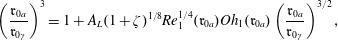 $$\begin{eqnarray}\left(\frac{\mathfrak{r}_{0a}}{\mathfrak{r}_{0\unicode[STIX]{x1D6FE}}}\right)^{3}=1+A_{L}(1+\unicode[STIX]{x1D701})^{1/8}Re_{1}^{1/4}(\mathfrak{r}_{0a})Oh_{1}(\mathfrak{r}_{0a})\left(\frac{\mathfrak{r}_{0a}}{\mathfrak{r}_{0\unicode[STIX]{x1D6FE}}}\right)^{3/2},\end{eqnarray}$$
under ‘laminar’ conditions,
 $A_{T}$
and
$A_{T}$
and
 $A_{L}$
being two unknown constants. The overall validity of an equivalent of (6.5) has been confirmed by Calabrese, Chang & Dang (Reference Calabrese, Chang and Dang1986) and Wang & Calabrese (Reference Wang and Calabrese1986), who performed extensive experiments with numerous liquid–liquid systems, varying
$A_{L}$
being two unknown constants. The overall validity of an equivalent of (6.5) has been confirmed by Calabrese, Chang & Dang (Reference Calabrese, Chang and Dang1986) and Wang & Calabrese (Reference Wang and Calabrese1986), who performed extensive experiments with numerous liquid–liquid systems, varying
 $\unicode[STIX]{x1D706}$
and
$\unicode[STIX]{x1D706}$
and
 $\unicode[STIX]{x1D6FE}$
over three and nearly two orders of magnitude respectively.
$\unicode[STIX]{x1D6FE}$
over three and nearly two orders of magnitude respectively.
The mean radii found under conditions (a), (b) and (c) defined above yield
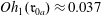 $Oh_{1}(\mathfrak{r}_{0a})\approx 0.037$
,
$Oh_{1}(\mathfrak{r}_{0a})\approx 0.037$
,
 $0.34$
and
$0.34$
and
 $1.05$
respectively. In the turbulent case,
$1.05$
respectively. In the turbulent case,
 $Re_{1}(\mathfrak{r})$
may be evaluated assuming that
$Re_{1}(\mathfrak{r})$
may be evaluated assuming that
 $\unicode[STIX]{x1D716}_{K}\propto V^{3}/R$
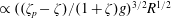 $\propto ((\unicode[STIX]{x1D701}_{p}-\unicode[STIX]{x1D701})/(1+\unicode[STIX]{x1D701})g)^{3/2}R^{1/2}$
, which yields
$\propto ((\unicode[STIX]{x1D701}_{p}-\unicode[STIX]{x1D701})/(1+\unicode[STIX]{x1D701})g)^{3/2}R^{1/2}$
, which yields
 $Re_{1}(\mathfrak{r})=((\unicode[STIX]{x1D701}_{p}-\unicode[STIX]{x1D701})/(\unicode[STIX]{x1D701}_{p}(1+\unicode[STIX]{x1D701})))^{1/2}Ar(\mathfrak{r}/R)^{4/3}$
. In the ‘laminar’ situation, one first has to identify the relevant outer scales that determine
$Re_{1}(\mathfrak{r})=((\unicode[STIX]{x1D701}_{p}-\unicode[STIX]{x1D701})/(\unicode[STIX]{x1D701}_{p}(1+\unicode[STIX]{x1D701})))^{1/2}Ar(\mathfrak{r}/R)^{4/3}$
. In the ‘laminar’ situation, one first has to identify the relevant outer scales that determine
 $\unicode[STIX]{x1D6E4}_{0}$
. The sphere settling velocity
$\unicode[STIX]{x1D6E4}_{0}$
. The sphere settling velocity
 $V$
and the thickness
$V$
and the thickness
 $\unicode[STIX]{x1D6FF}_{2}$
of the boundary layer that develops in the outer fluid along the tail seem to be natural candidates, yielding
$\unicode[STIX]{x1D6FF}_{2}$
of the boundary layer that develops in the outer fluid along the tail seem to be natural candidates, yielding
 $\unicode[STIX]{x1D6E4}_{0}=S=V/\unicode[STIX]{x1D6FF}_{2}$
, where
$\unicode[STIX]{x1D6E4}_{0}=S=V/\unicode[STIX]{x1D6FF}_{2}$
, where
 $S$
stands for the average shear rate in the boundary layer. Nevertheless, since the tail/outer-fluid interface is close to vertical, baroclinic effects are also likely to take place. Over the same distance
$S$
stands for the average shear rate in the boundary layer. Nevertheless, since the tail/outer-fluid interface is close to vertical, baroclinic effects are also likely to take place. Over the same distance
 $\unicode[STIX]{x1D6FF}_{2}$
(which is the smallest length scale involved in the system), the ratio of baroclinic to shear effects may be expressed through the Richardson number
$\unicode[STIX]{x1D6FF}_{2}$
(which is the smallest length scale involved in the system), the ratio of baroclinic to shear effects may be expressed through the Richardson number
 $Ri=N^{2}/S^{2}$
, with
$Ri=N^{2}/S^{2}$
, with
 $N^{2}=2(\unicode[STIX]{x1D70C}_{2}-\unicode[STIX]{x1D70C}_{1})/(\unicode[STIX]{x1D70C}_{2}+\unicode[STIX]{x1D70C}_{1})(g/\unicode[STIX]{x1D6FF}_{2})$
, and one might alternatively choose
$N^{2}=2(\unicode[STIX]{x1D70C}_{2}-\unicode[STIX]{x1D70C}_{1})/(\unicode[STIX]{x1D70C}_{2}+\unicode[STIX]{x1D70C}_{1})(g/\unicode[STIX]{x1D6FF}_{2})$
, and one might alternatively choose
 $\unicode[STIX]{x1D6E4}_{0}=N$
. The boundary layer thickness
$\unicode[STIX]{x1D6E4}_{0}=N$
. The boundary layer thickness
 $\unicode[STIX]{x1D6FF}_{2}(t)$
evolves as
$\unicode[STIX]{x1D6FF}_{2}(t)$
evolves as
 $\unicode[STIX]{x1D6FF}_{2}(t)=(\unicode[STIX]{x1D707}_{2}t/\unicode[STIX]{x1D70C}_{2})^{1/2}\propto (\unicode[STIX]{x1D707}_{2}L(t)/(\unicode[STIX]{x1D70C}_{2}V))^{1/2}$
, i.e.
$\unicode[STIX]{x1D6FF}_{2}(t)=(\unicode[STIX]{x1D707}_{2}t/\unicode[STIX]{x1D70C}_{2})^{1/2}\propto (\unicode[STIX]{x1D707}_{2}L(t)/(\unicode[STIX]{x1D70C}_{2}V))^{1/2}$
, i.e.
 $(RL(t)/Ar_{l})^{1/2}$
, where
$(RL(t)/Ar_{l})^{1/2}$
, where
 $L(t)$
is the depth (measured from the initial interface) reached by the sphere at the time
$L(t)$
is the depth (measured from the initial interface) reached by the sphere at the time
 $t$
when
$t$
when
 $\mathfrak{r}_{0a}$
is determined. Use of the above estimate for
$\mathfrak{r}_{0a}$
is determined. Use of the above estimate for
 $\unicode[STIX]{x1D6FF}_{2}$
reveals that the ratio
$\unicode[STIX]{x1D6FF}_{2}$
reveals that the ratio
 $N/S$
does not exceed a few per cent (
$N/S$
does not exceed a few per cent (
 $3\,\%$
in the case of the V5/water pair, which has the largest density contrast among the fluid systems in which fragmentation was observed). This confirms
$3\,\%$
in the case of the V5/water pair, which has the largest density contrast among the fluid systems in which fragmentation was observed). This confirms
 $S$
as the relevant choice to characterize the strain rate applied by the outer fluid to the tail, whereas baroclinic effects only play a minor role. Hence, with
$S$
as the relevant choice to characterize the strain rate applied by the outer fluid to the tail, whereas baroclinic effects only play a minor role. Hence, with
 $\unicode[STIX]{x1D6E4}_{0}=S=((\unicode[STIX]{x1D701}_{p}-\unicode[STIX]{x1D701})/(1+\unicode[STIX]{x1D701})gR)^{1/2}/\unicode[STIX]{x1D6FF}_{2}(t)$
, one finds
$\unicode[STIX]{x1D6E4}_{0}=S=((\unicode[STIX]{x1D701}_{p}-\unicode[STIX]{x1D701})/(1+\unicode[STIX]{x1D701})gR)^{1/2}/\unicode[STIX]{x1D6FF}_{2}(t)$
, one finds
 $Re_{1}(\mathfrak{r})=((\unicode[STIX]{x1D701}_{p}-\unicode[STIX]{x1D701})/(\unicode[STIX]{x1D701}_{p}(1+\unicode[STIX]{x1D701}))Ar_{l}(R/L))^{1/2}Ar(\mathfrak{r}/R)^{2}$
. Each of the two definitions of
$Re_{1}(\mathfrak{r})=((\unicode[STIX]{x1D701}_{p}-\unicode[STIX]{x1D701})/(\unicode[STIX]{x1D701}_{p}(1+\unicode[STIX]{x1D701}))Ar_{l}(R/L))^{1/2}Ar(\mathfrak{r}/R)^{2}$
. Each of the two definitions of
 $Re_{1}$
involves an arbitrary prefactor, but the latter does not vary among the three experimental sequences, so that it can be lumped into the corresponding constant
$Re_{1}$
involves an arbitrary prefactor, but the latter does not vary among the three experimental sequences, so that it can be lumped into the corresponding constant
 $A_{T}$
or
$A_{T}$
or
 $A_{L}$
.
$A_{L}$
.
With
 $\mathfrak{r}_{0a}$
,
$\mathfrak{r}_{0a}$
,
 $Oh_{1}(\mathfrak{r}_{0a})$
and
$Oh_{1}(\mathfrak{r}_{0a})$
and
 $Re_{1}(\mathfrak{r}_{0a})$
at hand in each case, (6.5) and (6.6) may be used to estimate
$Re_{1}(\mathfrak{r}_{0a})$
at hand in each case, (6.5) and (6.6) may be used to estimate
 $A_{T}$
and
$A_{T}$
and
 $A_{L}$
and possibly determine which scaling is the most appropriate. To this end, we employed the following procedure. First, noting that
$A_{L}$
and possibly determine which scaling is the most appropriate. To this end, we employed the following procedure. First, noting that
 $Oh_{1}$
is small in case (a), the corresponding
$Oh_{1}$
is small in case (a), the corresponding
 $\mathfrak{r}_{0a}$
is close to
$\mathfrak{r}_{0a}$
is close to
 $\mathfrak{r}_{0\unicode[STIX]{x1D6FE}}$
and may be used as an initial guess to determine the latter. Starting with this guess, we computed a first estimate of
$\mathfrak{r}_{0\unicode[STIX]{x1D6FE}}$
and may be used as an initial guess to determine the latter. Starting with this guess, we computed a first estimate of
 $\mathfrak{r}_{0\unicode[STIX]{x1D6FE}}$
for case (c) (in which
$\mathfrak{r}_{0\unicode[STIX]{x1D6FE}}$
for case (c) (in which
 $\unicode[STIX]{x1D6FE}$
is one order of magnitude smaller), using either (6.1) or (6.2), and extracted a first estimate of
$\unicode[STIX]{x1D6FE}$
is one order of magnitude smaller), using either (6.1) or (6.2), and extracted a first estimate of
 $A_{T}$
and
$A_{T}$
and
 $A_{L}$
by solving (6.5) and (6.6), still for case (c), which has the largest
$A_{L}$
by solving (6.5) and (6.6), still for case (c), which has the largest
 $Oh_{1}$
, and hence the largest sensitivity to viscous effects. Then, we used these values of
$Oh_{1}$
, and hence the largest sensitivity to viscous effects. Then, we used these values of
 $A_{T}$
and
$A_{T}$
and
 $A_{L}$
in (6.5) and (6.6) to obtain a first correction to
$A_{L}$
in (6.5) and (6.6) to obtain a first correction to
 $\mathfrak{r}_{0\unicode[STIX]{x1D6FE}}$
for case (a). We repeated this process until convergence, obtaining
$\mathfrak{r}_{0\unicode[STIX]{x1D6FE}}$
for case (a). We repeated this process until convergence, obtaining
 $A_{T}\approx 2.07$
(respectively
$A_{T}\approx 2.07$
(respectively
 $A_{L}\approx 2.18$
) and
$A_{L}\approx 2.18$
) and
 $\mathfrak{r}_{0\unicode[STIX]{x1D6FE}}=0.52$
mm (respectively
$\mathfrak{r}_{0\unicode[STIX]{x1D6FE}}=0.52$
mm (respectively
 $0.57~\text{mm}$
) in case (a), and hence
$0.57~\text{mm}$
) in case (a), and hence
 $\mathfrak{r}_{0\unicode[STIX]{x1D6FE}}=0.14$
mm (respectively
$\mathfrak{r}_{0\unicode[STIX]{x1D6FE}}=0.14$
mm (respectively
 $0.275~\text{mm}$
) in case (c). Since the interfacial tension is virtually the same in fluid pairs (a) and (b), so is
$0.275~\text{mm}$
) in case (c). Since the interfacial tension is virtually the same in fluid pairs (a) and (b), so is
 $\mathfrak{r}_{0\unicode[STIX]{x1D6FE}}$
, and we could then make use of the previously determined
$\mathfrak{r}_{0\unicode[STIX]{x1D6FE}}$
, and we could then make use of the previously determined
 $\mathfrak{r}_{0\unicode[STIX]{x1D6FE}}$
to assess which value of
$\mathfrak{r}_{0\unicode[STIX]{x1D6FE}}$
to assess which value of
 $A_{T}$
(respectively
$A_{T}$
(respectively
 $A_{L}$
) is necessary for (6.5) (respectively (6.6)) to predict the experimentally observed value of
$A_{L}$
) is necessary for (6.5) (respectively (6.6)) to predict the experimentally observed value of
 $\mathfrak{r}_{eq}$
in case (b). This procedure yielded
$\mathfrak{r}_{eq}$
in case (b). This procedure yielded
 $A_{T}\approx 1.30$
and
$A_{T}\approx 1.30$
and
 $A_{L}\approx 1.80$
. Hence, the two values of
$A_{L}\approx 1.80$
. Hence, the two values of
 $A_{L}$
obtained from cases (a) and (c) are close to one another (
$A_{L}$
obtained from cases (a) and (c) are close to one another (
 $20\,\%$
difference), whereas those of
$20\,\%$
difference), whereas those of
 $A_{T}$
clearly differ by nearly
$A_{T}$
clearly differ by nearly
 $60\,\%$
. This suggests that, in the flow under consideration, the appropriate scaling almost corresponds to ‘laminar’ conditions, the larger ‘fully turbulent’ exponents associated with the physical properties
$60\,\%$
. This suggests that, in the flow under consideration, the appropriate scaling almost corresponds to ‘laminar’ conditions, the larger ‘fully turbulent’ exponents associated with the physical properties
 $\unicode[STIX]{x1D6FE}$
and
$\unicode[STIX]{x1D6FE}$
and
 $\unicode[STIX]{x1D707}_{1}$
in (6.1) and (6.3) overestimating the sensitivity of
$\unicode[STIX]{x1D707}_{1}$
in (6.1) and (6.3) overestimating the sensitivity of
 $\mathfrak{r}_{0a}$
to these properties. This conclusion supports the view that the shear resulting from the boundary layer that develops around the tail is the main source of fragmentation under the present conditions. This does not mean that turbulence is absent from the wake, but rather that its intensity is not large enough in the relevant range of scales for the resulting strain rates to compete with the strong shear provided by the boundary layer. This situation is reminiscent of the findings of Eastwood, Armi & Lasheras (Reference Eastwood, Armi and Lasheras2004), who performed experiments in a turbulent water jet with known characteristics, in which small amounts of various liquids were released on the centreline through a needle. They observed that droplets resulting from the breakup process did not follow the Hinze–Kolmogorov scaling (6.1), whereas bubbles produced in the same device using the same protocol did, as previously noticed by Martinez-Bazán, Montañes & Lasheras (Reference Martinez-Bazán, Montañes and Lasheras1999). They attributed this remarkable difference to the fact that the small-scale nearly isotropic turbulent motions present in the jet are sufficiently energetic to break air filaments, whereas liquid filaments with much larger densities and viscosities can only break under the action of large-scale organized vortices.
$\mathfrak{r}_{0a}$
to these properties. This conclusion supports the view that the shear resulting from the boundary layer that develops around the tail is the main source of fragmentation under the present conditions. This does not mean that turbulence is absent from the wake, but rather that its intensity is not large enough in the relevant range of scales for the resulting strain rates to compete with the strong shear provided by the boundary layer. This situation is reminiscent of the findings of Eastwood, Armi & Lasheras (Reference Eastwood, Armi and Lasheras2004), who performed experiments in a turbulent water jet with known characteristics, in which small amounts of various liquids were released on the centreline through a needle. They observed that droplets resulting from the breakup process did not follow the Hinze–Kolmogorov scaling (6.1), whereas bubbles produced in the same device using the same protocol did, as previously noticed by Martinez-Bazán, Montañes & Lasheras (Reference Martinez-Bazán, Montañes and Lasheras1999). They attributed this remarkable difference to the fact that the small-scale nearly isotropic turbulent motions present in the jet are sufficiently energetic to break air filaments, whereas liquid filaments with much larger densities and viscosities can only break under the action of large-scale organized vortices.
Assuming an ‘averaged’ value
 $A_{L}=2.0$
, (6.6) predicts
$A_{L}=2.0$
, (6.6) predicts
 $\mathfrak{r}_{0a}=0.625$
,
$\mathfrak{r}_{0a}=0.625$
,
 $0.89$
and
$0.89$
and
 $0.75$
mm for cases (a), (b) and (c) respectively. Given the
$0.75$
mm for cases (a), (b) and (c) respectively. Given the
 $0.08$
mm uncertainty on the optical determination of
$0.08$
mm uncertainty on the optical determination of
 $\mathfrak{r}_{0a}$
and the significant statistical uncertainty due to the limited sample of drops we considered, these predictions may be considered to compare well with the experimental values of
$\mathfrak{r}_{0a}$
and the significant statistical uncertainty due to the limited sample of drops we considered, these predictions may be considered to compare well with the experimental values of
 $\mathfrak{r}_{0a}=0.625$
,
$\mathfrak{r}_{0a}=0.625$
,
 $0.84$
and
$0.84$
and
 $0.78$
mm in all three cases. Hence, (6.5) with
$0.78$
mm in all three cases. Hence, (6.5) with
 $A_{L}=2.0$
appears to be a simple but potentially useful model for predicting the average size of drops resulting from fragmentation in ‘quasi-laminar’ liquid–liquid systems involving significant viscous effects in the dispersed phase, at least down to
$A_{L}=2.0$
appears to be a simple but potentially useful model for predicting the average size of drops resulting from fragmentation in ‘quasi-laminar’ liquid–liquid systems involving significant viscous effects in the dispersed phase, at least down to
 $\unicode[STIX]{x1D706}=O(10^{-2})$
. More experiments covering a wider range of physical properties and flow conditions, supplemented by extensive data processing, are of course necessary to confirm this provisional conclusion.
$\unicode[STIX]{x1D706}=O(10^{-2})$
. More experiments covering a wider range of physical properties and flow conditions, supplemented by extensive data processing, are of course necessary to confirm this provisional conclusion.
7 Summary
In this paper, we reported on a series of experiments aimed at characterizing various aspects of the breakthrough process of a rigid sphere settling across a two-layer system made of two superimposed immiscible Newtonian fluids, namely a thick layer of silicone oil on top of a water or glycerin+water bath. By varying the physical characteristics of the two fluids, especially their viscosities, employing spheres made of different materials and varying their diameter, we were able to produce conditions under which the viscosity ratio and the ratio of inertia to viscous effects acting on the sphere spanned almost four orders of magnitude, while the solid-to-fluid density contrast spanned more than one order of magnitude.
Under most flow conditions, once the sphere reaches the interface, it penetrates more or less easily into the lower fluid, while pulling a column or tail of the upper fluid which elongates as time proceeds. However, in several configurations, small light spheres remain trapped steadily at the interface. In the opposite limit corresponding to the heaviest and largest spheres, the column is often observed to disintegrate quickly into a very large number of droplets, which corresponds to a situation of liquid–liquid fragmentation. In between these two limits, the characteristics of the column deeply depend on the viscosity ratio and Archimedes number, but also on the density contrast between the two fluids. In particular, in the region close to the sphere, the geometry of the column carries the footprint of the wake structure that develops during the time period in which the sphere settles in the upper fluid. That is, the bottom part of the column displays a fully three-dimensional geometry with hairpin-like regions for Archimedes numbers of
 $O(10^{2})$
or more, which is in line with the available knowledge regarding the breakdown of wake axisymmetry past a sphere translating in a uniform fluid. For lower Archimedes numbers, the column remains axisymmetric. When the viscosity of the lower fluid is large, it tends to pinch off close to the initial position of the interface when the sphere is light and small enough, and, for
$O(10^{2})$
or more, which is in line with the available knowledge regarding the breakdown of wake axisymmetry past a sphere translating in a uniform fluid. For lower Archimedes numbers, the column remains axisymmetric. When the viscosity of the lower fluid is large, it tends to pinch off close to the initial position of the interface when the sphere is light and small enough, and, for
 $Ar$
in the range
$Ar$
in the range
 $[10,100]$
, exhibits a thick cylindrical bottom part reflecting the geometry of the standing eddy. In contrast, when the viscosity of the lower fluid is low, the column breaks up close to the top of the sphere, which then falls with an oil drop attached to its top half. We derived scaling laws for the pinch-off time which rationalize experimental observations, showing, in particular, that the transition from ‘shallow’ pinch-off close to the interface to ‘deep’ pinch-off close to the sphere takes place when the Bond number exceeds a critical value that depends on the sphere inertia. These scaling laws also qualitatively explain how, by forcing the sphere to accelerate or decelerate during the breakthrough, the viscosity and fluid density contrasts act to favour a ‘deep’ or a ‘shallow’ pinch-off respectively.
$[10,100]$
, exhibits a thick cylindrical bottom part reflecting the geometry of the standing eddy. In contrast, when the viscosity of the lower fluid is low, the column breaks up close to the top of the sphere, which then falls with an oil drop attached to its top half. We derived scaling laws for the pinch-off time which rationalize experimental observations, showing, in particular, that the transition from ‘shallow’ pinch-off close to the interface to ‘deep’ pinch-off close to the sphere takes place when the Bond number exceeds a critical value that depends on the sphere inertia. These scaling laws also qualitatively explain how, by forcing the sphere to accelerate or decelerate during the breakthrough, the viscosity and fluid density contrasts act to favour a ‘deep’ or a ‘shallow’ pinch-off respectively.
An important conclusion that may be drawn from the present observations is that, as far as the sphere remains connected to the tail, the dynamics of its wake is driven by the properties (especially the viscosity) of the upper fluid, not by those of the lower one. This is especially clear when the viscosity of the upper fluid is much larger than that of the lower one, in which case the tail remains axisymmetric until possible instabilities develop at the interface between the two fluids. When the sphere inertia is large enough, such instabilities arise at the bottom of the tail, leading to the formation of thin axisymmetric corollas surrounding its central part and propagating upwards. This specific configuration precedes the onset of fragmentation, which occurs when the sphere inertia is increased somewhat further. We rationalized the ‘zoology’ of configurations encountered in the various pairs of fluids in two regime maps based on the dimensionless parameters most relevant to ‘small light’ and ‘large heavy’ spheres respectively.
The rest of the paper focused on three specific phenomena encountered during the course of the experiments, namely flotation of light spheres at the interface, characteristics of drops remaining attached to the sphere after the tail has pinched off and wake fragmentation.
Light enough spheres were observed to float steadily at the interface in several pairs of fluids. To rationalize these observations, we derived a necessary criterion based on a quasi-steady force balance in which only the capillary force and the net buoyancy force on the sphere, which includes a contribution from the meniscus, were taken into account. Comparison with experimental data showed that, under most conditions, this criterion predicts accurately the critical characteristics, i.e. density and radius, making spheres able to float. However, we also identified some situations in which spheres succeed in crossing the interface although this criterion is satisfied. We found that this occurs when the viscosity and density contrasts are such that the sphere experiences a strong deceleration when it reaches the interface and stops within a short distance. In such cases, the collapse of the wake results in a supplementary downward force which still acts for some time after the sphere has momentarily stopped, making it able to eventually overcome capillary and buoyancy effects.
In cases where the tail pinches off close to the sphere and a drop remains attached to its top part, we attempted to clarify the way in which the drop volume varies with the characteristics of the fluids and the sphere. For that purpose, we established the force budget on the drop itself and on the compound body made of the sphere plus the drop. This allowed us to obtain qualitative predictions in two limiting cases. When the densities of the two fluids are close (
 $\unicode[STIX]{x1D701}\ll 1$
) and the viscosity of the lower fluid is much smaller than that of the upper one (
$\unicode[STIX]{x1D701}\ll 1$
) and the viscosity of the lower fluid is much smaller than that of the upper one (
 $\unicode[STIX]{x1D706}\ll 1$
), this volume is governed by the balance between the capillary force and the drag force acting on the drop. In that case, the drop volume increases with the sphere size and the solid-to-fluid density ratio, and decreases with the interfacial tension. The situation is more complex when the fluid density contrast is significant. Although the corresponding configurations keep connections with the classical static pendant drop problem, so that the drop volume decreases as the Bond number is increased, we observed that this volume remains sensitive to the solid-to-fluid density ratio. Capillary, buoyancy and viscous forces are then in balance and we could only draw firm conclusions from this balance when the lower fluid had a much larger viscosity than the upper one (
$\unicode[STIX]{x1D706}\ll 1$
), this volume is governed by the balance between the capillary force and the drag force acting on the drop. In that case, the drop volume increases with the sphere size and the solid-to-fluid density ratio, and decreases with the interfacial tension. The situation is more complex when the fluid density contrast is significant. Although the corresponding configurations keep connections with the classical static pendant drop problem, so that the drop volume decreases as the Bond number is increased, we observed that this volume remains sensitive to the solid-to-fluid density ratio. Capillary, buoyancy and viscous forces are then in balance and we could only draw firm conclusions from this balance when the lower fluid had a much larger viscosity than the upper one (
 $\unicode[STIX]{x1D706}\gg 1$
), in which case the viscous force on the drop was shown to act as an additional buoyancy force, decreasing the drop volume as
$\unicode[STIX]{x1D706}\gg 1$
), in which case the viscous force on the drop was shown to act as an additional buoyancy force, decreasing the drop volume as
 $\unicode[STIX]{x1D701}_{p}/\unicode[STIX]{x1D701}$
increased for a given
$\unicode[STIX]{x1D701}_{p}/\unicode[STIX]{x1D701}$
increased for a given
 $Bo$
. Experimental data obtained in the various pairs of fluids confirmed these predictions.
$Bo$
. Experimental data obtained in the various pairs of fluids confirmed these predictions.
In the last part, we considered the fragmentation process observed in the fluid column pulled by the largest and heaviest spheres when they sink in a low-viscosity lower fluid, provided that the viscosity of the upper fluid is not ‘too’ large. We processed the images obtained with different pairs of fluids to determine the average size of the resulting oil droplets. With these results at hand, we developed a model based on dimensional analysis arguments to better understand how the effects of interfacial tension and tail viscosity combine to influence the mean droplet size. We did so by considering both a turbulent and a quasi-laminar scaling, the difference between the two being that the strain rate in the outer fluid at the droplet scale is scale-dependent in the former case while it is governed by the thickness of the boundary layer that surrounds the tail in the latter case. In each case, the corresponding model involves only one empirical parameter. Comparison of the two series of predictions with experimental data revealed that the quasi-laminar scaling is the only one predicting correctly the mild variations of the droplet size observed when viscosity and interfacial tension are varied by one order of magnitude, which gives credit to the scenario of a fragmentation process driven by the boundary layer.
The present paper left the dynamics of the sphere and tail almost untouched: we did not examine the evolution of the sphere velocity during the breakthrough process, or that of the tail volume. Similarly, the post-pinch-off dynamics of the tail was not considered, although it can be expected that it exhibits very different features, depending on the viscosity contrast between the two fluids. This is the subject of the companion paper.
Acknowledgements
We thank G. Ehses for having taken care of all experimental aspects and S. Cazin for his expert technical assistance with the optical and high-speed imaging acquisition systems. J.-L.P.’s fellowship was provided by the Délégation Générale de l’Armement, whose financial support is greatly appreciated.
Supplementary movies
Supplementary movies are available at https://doi.org/10.1017/jfm.2017.747.
Appendix A. Mechanisms governing the pinch-off style
Derivation of a quantitative model aimed at predicting the pinch-off location is beyond the scope of this paper. As the inner and outer fluids have comparable inertias, the dynamics is much more complex than in the case of air cavities created by a sphere impacting a free surface, where simple models based on the radial dynamics of the outer flow, assumed to be irrotational, have proved successful (Duclaux et al.
Reference Duclaux, Caillé, Duez, Ybert, Bocquet and Clanet2007; Aristoff & Bush Reference Aristoff and Bush2009). Nevertheless, qualitative arguments may be developed to help to interpret present observations. For this, let us consider that at a distance
 $z$
below the interface (
$z$
below the interface (
 $z<0$
), the tail radius is
$z<0$
), the tail radius is
 ${\mathcal{R}}(z,t)$
and the cross-sectional average of the vertical fluid velocity
${\mathcal{R}}(z,t)$
and the cross-sectional average of the vertical fluid velocity
 $W(r,z,t)$
within the tail is
$W(r,z,t)$
within the tail is
 $\overline{W}(z,t)$
. The radial inertial force acting on the tail, which involves the acceleration
$\overline{W}(z,t)$
. The radial inertial force acting on the tail, which involves the acceleration
 $\text{d}^{2}{\mathcal{R}}/\text{d}t^{2}$
, is driven by the vertical variation of the sum of capillary, buoyancy and dynamic pressure contributions, which can be modelled in a first approach as
$\text{d}^{2}{\mathcal{R}}/\text{d}t^{2}$
, is driven by the vertical variation of the sum of capillary, buoyancy and dynamic pressure contributions, which can be modelled in a first approach as
 $\unicode[STIX]{x2202}_{z}\{\unicode[STIX]{x1D6FE}/{\mathcal{R}}-(\unicode[STIX]{x1D70C}_{2}-\unicode[STIX]{x1D70C}_{1})gz+(1/2)\unicode[STIX]{x1D70C}_{1}\overline{W}^{2}\}$
, assuming that the tail curvature in the vertical diametrical plane is small and neglecting effects due to possible local velocity differences
$\unicode[STIX]{x2202}_{z}\{\unicode[STIX]{x1D6FE}/{\mathcal{R}}-(\unicode[STIX]{x1D70C}_{2}-\unicode[STIX]{x1D70C}_{1})gz+(1/2)\unicode[STIX]{x1D70C}_{1}\overline{W}^{2}\}$
, assuming that the tail curvature in the vertical diametrical plane is small and neglecting effects due to possible local velocity differences
 $W-\overline{W}$
within the tail (these effects can actually become significant when
$W-\overline{W}$
within the tail (these effects can actually become significant when
 $\unicode[STIX]{x1D706}$
is large, since the velocity distribution is then close to a Poiseuille profile, where
$\unicode[STIX]{x1D706}$
is large, since the velocity distribution is then close to a Poiseuille profile, where
 $|W/\overline{W}|$
may locally be up to
$|W/\overline{W}|$
may locally be up to
 $1/2$
). As both fluids have comparable densities, the radial acceleration term is weighted by a combination of their densities, say
$1/2$
). As both fluids have comparable densities, the radial acceleration term is weighted by a combination of their densities, say
 $(1-k)\unicode[STIX]{x1D70C}_{1}+k\unicode[STIX]{x1D70C}_{2}=\unicode[STIX]{x1D70C}_{1}(1+k\unicode[STIX]{x1D701})$
, where
$(1-k)\unicode[STIX]{x1D70C}_{1}+k\unicode[STIX]{x1D70C}_{2}=\unicode[STIX]{x1D70C}_{1}(1+k\unicode[STIX]{x1D701})$
, where
 $k$
is an
$k$
is an
 $O(1)$
constant (
$O(1)$
constant (
 $0<k<1$
) that depends on the nature of the two flows and of their couplings.
$0<k<1$
) that depends on the nature of the two flows and of their couplings.
If
 $\overline{W}$
varies slowly with
$\overline{W}$
varies slowly with
 $z$
and
$z$
and
 $t$
, two limit cases may occur. At small depths, buoyancy effects are negligible, so that pinch-off is driven by interfacial tension. Balancing the capillary pressure gradient and radial acceleration terms reveals that the characteristic pinch-off time,
$t$
, two limit cases may occur. At small depths, buoyancy effects are negligible, so that pinch-off is driven by interfacial tension. Balancing the capillary pressure gradient and radial acceleration terms reveals that the characteristic pinch-off time,
 $\unicode[STIX]{x1D70F}_{\unicode[STIX]{x1D6FE}}$
, required to reduce
$\unicode[STIX]{x1D70F}_{\unicode[STIX]{x1D6FE}}$
, required to reduce
 ${\mathcal{R}}$
from an
${\mathcal{R}}$
from an
 $O(R)$
initial value to zero scales as
$O(R)$
initial value to zero scales as
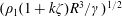 $(\unicode[STIX]{x1D70C}_{1}(1+k\unicode[STIX]{x1D701})R^{3}/\unicode[STIX]{x1D6FE})^{1/2}$
. Hence, the dimensionless time
$(\unicode[STIX]{x1D70C}_{1}(1+k\unicode[STIX]{x1D701})R^{3}/\unicode[STIX]{x1D6FE})^{1/2}$
. Hence, the dimensionless time
 $\unicode[STIX]{x1D70F}_{\unicode[STIX]{x1D6FE}}^{\ast }=\unicode[STIX]{x1D70F}_{\unicode[STIX]{x1D6FE}}V_{c}/R$
, normalized by the characteristic sphere velocity scale
$\unicode[STIX]{x1D70F}_{\unicode[STIX]{x1D6FE}}^{\ast }=\unicode[STIX]{x1D70F}_{\unicode[STIX]{x1D6FE}}V_{c}/R$
, normalized by the characteristic sphere velocity scale
 $V_{c}=(\unicode[STIX]{x1D701}_{p}gR)^{1/2}$
and radius
$V_{c}=(\unicode[STIX]{x1D701}_{p}gR)^{1/2}$
and radius
 $R$
, is such that
$R$
, is such that
 $\unicode[STIX]{x1D70F}_{\unicode[STIX]{x1D6FE}}^{\ast }\sim \{(1+k\unicode[STIX]{x1D701})(\unicode[STIX]{x1D701}_{p}/\unicode[STIX]{x1D701})Bo\}^{1/2}$
. Since the sphere stands at depth
$\unicode[STIX]{x1D70F}_{\unicode[STIX]{x1D6FE}}^{\ast }\sim \{(1+k\unicode[STIX]{x1D701})(\unicode[STIX]{x1D701}_{p}/\unicode[STIX]{x1D701})Bo\}^{1/2}$
. Since the sphere stands at depth
 $|z|_{c}\sim V_{c}\unicode[STIX]{x1D70F}_{\unicode[STIX]{x1D6FE}}$
when pinch-off occurs,
$|z|_{c}\sim V_{c}\unicode[STIX]{x1D70F}_{\unicode[STIX]{x1D6FE}}$
when pinch-off occurs,
 $\unicode[STIX]{x1D70F}_{\unicode[STIX]{x1D6FE}}^{\ast }$
represents the dimensionless length of the tail by the pinch-off time. Conversely, buoyancy is dominant at depths such that
$\unicode[STIX]{x1D70F}_{\unicode[STIX]{x1D6FE}}^{\ast }$
represents the dimensionless length of the tail by the pinch-off time. Conversely, buoyancy is dominant at depths such that
 $|z|/R\gg Bo^{-1}$
. Keeping in mind that the sphere has to settle in the lower fluid during a time
$|z|/R\gg Bo^{-1}$
. Keeping in mind that the sphere has to settle in the lower fluid during a time
 $t\sim |z|/V_{c}$
before reaching a depth
$t\sim |z|/V_{c}$
before reaching a depth
 $|z|$
, the balance between the buoyancy and the radial acceleration terms indicates that the corresponding dimensionless pinch-off time,
$|z|$
, the balance between the buoyancy and the radial acceleration terms indicates that the corresponding dimensionless pinch-off time,
 $\unicode[STIX]{x1D70F}_{g}^{\ast }$
, scales as
$\unicode[STIX]{x1D70F}_{g}^{\ast }$
, scales as
 $\unicode[STIX]{x1D70F}_{g}^{\ast }\sim \{(1+k\unicode[STIX]{x1D701})(\unicode[STIX]{x1D701}_{p}/\unicode[STIX]{x1D701})\}^{1/3}$
. A shallow (respectively deep) seal configuration is observed only if
$\unicode[STIX]{x1D70F}_{g}^{\ast }\sim \{(1+k\unicode[STIX]{x1D701})(\unicode[STIX]{x1D701}_{p}/\unicode[STIX]{x1D701})\}^{1/3}$
. A shallow (respectively deep) seal configuration is observed only if
 $\unicode[STIX]{x1D70F}_{\unicode[STIX]{x1D6FE}}^{\ast }<\unicode[STIX]{x1D70F}_{g}^{\ast }$
(respectively
$\unicode[STIX]{x1D70F}_{\unicode[STIX]{x1D6FE}}^{\ast }<\unicode[STIX]{x1D70F}_{g}^{\ast }$
(respectively
 $\unicode[STIX]{x1D70F}_{\unicode[STIX]{x1D6FE}}^{\ast }>\unicode[STIX]{x1D70F}_{g}^{\ast }$
). Hence, the transition between the two regimes is expected to take place at a critical Bond number
$\unicode[STIX]{x1D70F}_{\unicode[STIX]{x1D6FE}}^{\ast }>\unicode[STIX]{x1D70F}_{g}^{\ast }$
). Hence, the transition between the two regimes is expected to take place at a critical Bond number
 $Bo_{t}\sim \{(1+k\unicode[STIX]{x1D701})(\unicode[STIX]{x1D701}_{p}/\unicode[STIX]{x1D701})\}^{-1/3}$
, only deep (respectively shallow) seal being possible at larger (respectively smaller) Bond numbers. For small fluid density contrasts (
$Bo_{t}\sim \{(1+k\unicode[STIX]{x1D701})(\unicode[STIX]{x1D701}_{p}/\unicode[STIX]{x1D701})\}^{-1/3}$
, only deep (respectively shallow) seal being possible at larger (respectively smaller) Bond numbers. For small fluid density contrasts (
 $\unicode[STIX]{x1D701}\ll 1$
), the above predictions reduce to
$\unicode[STIX]{x1D701}\ll 1$
), the above predictions reduce to
 $$\begin{eqnarray}\unicode[STIX]{x1D70F}_{\unicode[STIX]{x1D6FE}}^{\ast }\sim ((\unicode[STIX]{x1D701}_{p}/\unicode[STIX]{x1D701})Bo)^{1/2},\quad \unicode[STIX]{x1D70F}_{g}^{\ast }\sim (\unicode[STIX]{x1D701}_{p}/\unicode[STIX]{x1D701})^{1/3}\quad \text{and}\quad Bo_{t}\sim (\unicode[STIX]{x1D701}_{p}/\unicode[STIX]{x1D701})^{-1/3}\end{eqnarray}$$
respectively. In contrast, if the lower fluid is much denser than the upper one, as in air–water impacts, they become
 $\unicode[STIX]{x1D70F}_{\unicode[STIX]{x1D6FE}}^{\ast }\sim (\unicode[STIX]{x1D701}_{p}Bo)^{1/2}$
,
$\unicode[STIX]{x1D70F}_{\unicode[STIX]{x1D6FE}}^{\ast }\sim (\unicode[STIX]{x1D701}_{p}Bo)^{1/2}$
,
 $\unicode[STIX]{x1D70F}_{g}^{\ast }\sim \unicode[STIX]{x1D701}_{p}^{1/3}$
and
$\unicode[STIX]{x1D70F}_{g}^{\ast }\sim \unicode[STIX]{x1D701}_{p}^{1/3}$
and
 $Bo_{t}\sim \unicode[STIX]{x1D701}_{p}^{-1/3}$
respectively. In that case, noting that
$Bo_{t}\sim \unicode[STIX]{x1D701}_{p}^{-1/3}$
respectively. In that case, noting that
 $\unicode[STIX]{x1D701}_{p}^{1/2}=V_{c}/(gR)^{1/2}$
may be interpreted as the Froude number of the system, say
$\unicode[STIX]{x1D701}_{p}^{1/2}=V_{c}/(gR)^{1/2}$
may be interpreted as the Froude number of the system, say
 $Fr$
, and introducing the Weber number
$Fr$
, and introducing the Weber number
 $We=\unicode[STIX]{x1D70C}_{2}V_{c}^{2}R/\unicode[STIX]{x1D6FE}=BoFr^{2}$
, one also has
$We=\unicode[STIX]{x1D70C}_{2}V_{c}^{2}R/\unicode[STIX]{x1D6FE}=BoFr^{2}$
, one also has
 $\unicode[STIX]{x1D70F}_{\unicode[STIX]{x1D6FE}}^{\ast }\sim We^{1/2}$
and
$\unicode[STIX]{x1D70F}_{\unicode[STIX]{x1D6FE}}^{\ast }\sim We^{1/2}$
and
 $\unicode[STIX]{x1D70F}_{g}^{\ast }\sim Fr^{2/3}$
, which yields a critical Bond number
$\unicode[STIX]{x1D70F}_{g}^{\ast }\sim Fr^{2/3}$
, which yields a critical Bond number
 $Bo_{t}\sim We^{-1/2}$
. The latter three scalings agree with predictions derived by Aristoff & Bush (Reference Aristoff and Bush2009) in the case of cylindrical cavities. It should be noted that viscous stresses at the tail surface were disregarded throughout the above reasoning. However, they of course play a role if their magnitude comes to be comparable to that of inertial contributions. The ratio of the radial acceleration term to the
$Bo_{t}\sim We^{-1/2}$
. The latter three scalings agree with predictions derived by Aristoff & Bush (Reference Aristoff and Bush2009) in the case of cylindrical cavities. It should be noted that viscous stresses at the tail surface were disregarded throughout the above reasoning. However, they of course play a role if their magnitude comes to be comparable to that of inertial contributions. The ratio of the radial acceleration term to the
 $z$
-derivative of the normal viscous stress provided by the outer fluid results in a viscous time scale
$z$
-derivative of the normal viscous stress provided by the outer fluid results in a viscous time scale
 $\unicode[STIX]{x1D70F}_{v}\sim \unicode[STIX]{x1D70C}_{1}(1+k\unicode[STIX]{x1D701})R^{2}/\unicode[STIX]{x1D707}_{2}$
, i.e.
$\unicode[STIX]{x1D70F}_{v}\sim \unicode[STIX]{x1D70C}_{1}(1+k\unicode[STIX]{x1D701})R^{2}/\unicode[STIX]{x1D707}_{2}$
, i.e.
 $\unicode[STIX]{x1D70F}_{v}^{\ast }\sim (1+k\unicode[STIX]{x1D701})Ar/\unicode[STIX]{x1D706}$
(
$\unicode[STIX]{x1D70F}_{v}^{\ast }\sim (1+k\unicode[STIX]{x1D701})Ar/\unicode[STIX]{x1D706}$
(
 ${\approx}Ar_{l}$
when
${\approx}Ar_{l}$
when
 $\unicode[STIX]{x1D701}\ll 1$
). Hence, the above scalings are valid only as far as
$\unicode[STIX]{x1D701}\ll 1$
). Hence, the above scalings are valid only as far as
 $\unicode[STIX]{x1D70F}_{v}^{\ast }\gg \text{max}(\unicode[STIX]{x1D70F}_{\unicode[STIX]{x1D6FE}}^{\ast },\unicode[STIX]{x1D70F}_{g}^{\ast })$
, which requires large enough
$\unicode[STIX]{x1D70F}_{v}^{\ast }\gg \text{max}(\unicode[STIX]{x1D70F}_{\unicode[STIX]{x1D6FE}}^{\ast },\unicode[STIX]{x1D70F}_{g}^{\ast })$
, which requires large enough
 $Ar_{l}$
.
$Ar_{l}$
.
The above reasoning assumes that the sphere settles through the lower fluid with a constant velocity equal to the terminal velocity
 $V_{T1}$
it acquired before reaching the interface, which is generally barely realistic. Effects of the deceleration of a sphere impacting a free surface were examined in detail by Aristoff et al. (Reference Aristoff, Truscott, Techet and Bush2010). Here, changes in the sphere velocity are expected to influence the pinch-off position because the average fluid velocity
$V_{T1}$
it acquired before reaching the interface, which is generally barely realistic. Effects of the deceleration of a sphere impacting a free surface were examined in detail by Aristoff et al. (Reference Aristoff, Truscott, Techet and Bush2010). Here, changes in the sphere velocity are expected to influence the pinch-off position because the average fluid velocity
 $\overline{W}(z,t)$
within the bottom part of the tail is necessarily close to the sphere velocity
$\overline{W}(z,t)$
within the bottom part of the tail is necessarily close to the sphere velocity
 $V(t)$
at all times. Expanding
$V(t)$
at all times. Expanding
 $\overline{W}(z,t)$
in the form
$\overline{W}(z,t)$
in the form
 $\overline{W}(z,t)\approx \overline{W}_{0}(t)+z\overline{W}_{z0}(t)+\cdots \,$
, with
$\overline{W}(z,t)\approx \overline{W}_{0}(t)+z\overline{W}_{z0}(t)+\cdots \,$
, with
 $\overline{W}_{0}(t)=\overline{W}(z=0,t)$
and
$\overline{W}_{0}(t)=\overline{W}(z=0,t)$
and
 $\overline{W}_{z0}(t)=(\unicode[STIX]{x2202}_{z}\overline{W})(z=0,t)$
, the dynamic pressure within the tail is seen to comprise a contribution
$\overline{W}_{z0}(t)=(\unicode[STIX]{x2202}_{z}\overline{W})(z=0,t)$
, the dynamic pressure within the tail is seen to comprise a contribution
 $\unicode[STIX]{x1D70C}_{1}(\overline{W}_{0}\overline{W}_{z0})z$
varying linearly with depth (the quadratic contribution
$\unicode[STIX]{x1D70C}_{1}(\overline{W}_{0}\overline{W}_{z0})z$
varying linearly with depth (the quadratic contribution
 $(1/2)\unicode[STIX]{x1D70C}_{1}(\overline{W}_{z0}z)^{2}$
and higher-order terms in the expansion may be neglected as far as the relative variation of
$(1/2)\unicode[STIX]{x1D70C}_{1}(\overline{W}_{z0}z)^{2}$
and higher-order terms in the expansion may be neglected as far as the relative variation of
 $\overline{W}$
over the range of
$\overline{W}$
over the range of
 $z$
of interest remains small). The above linear term may be regarded as an additional buoyancy effect. More precisely, one can define the dimensionless acceleration ratio
$z$
of interest remains small). The above linear term may be regarded as an additional buoyancy effect. More precisely, one can define the dimensionless acceleration ratio
 $\unicode[STIX]{x1D712}=-g^{-1}\overline{W}_{0}\overline{W}_{z0}$
, and write the sphere velocity in the form
$\unicode[STIX]{x1D712}=-g^{-1}\overline{W}_{0}\overline{W}_{z0}$
, and write the sphere velocity in the form
 $V(t)=V_{T1}{\mathcal{F}}(t)$
, with
$V(t)=V_{T1}{\mathcal{F}}(t)$
, with
 ${\mathcal{F}}(0)=1$
, so that the effective buoyancy contribution involved in the evaluation of the characteristic time
${\mathcal{F}}(0)=1$
, so that the effective buoyancy contribution involved in the evaluation of the characteristic time
 $\unicode[STIX]{x1D70F}_{g}$
is written as
$\unicode[STIX]{x1D70F}_{g}$
is written as
 $-\unicode[STIX]{x1D70C}_{1}\unicode[STIX]{x1D701}gz(1+\unicode[STIX]{x1D701}^{-1}\unicode[STIX]{x1D712})$
. Instead of
$-\unicode[STIX]{x1D70C}_{1}\unicode[STIX]{x1D701}gz(1+\unicode[STIX]{x1D701}^{-1}\unicode[STIX]{x1D712})$
. Instead of
 $\unicode[STIX]{x1D70F}_{g}^{\ast }\sim \{(1+k\unicode[STIX]{x1D701})(\unicode[STIX]{x1D701}_{p}/\unicode[STIX]{x1D701})\}^{1/3}$
, one then has
$\unicode[STIX]{x1D70F}_{g}^{\ast }\sim \{(1+k\unicode[STIX]{x1D701})(\unicode[STIX]{x1D701}_{p}/\unicode[STIX]{x1D701})\}^{1/3}$
, one then has
 $\unicode[STIX]{x1D70F}_{g}^{\ast }\sim \{\unicode[STIX]{x1D701}_{p}(1+k\unicode[STIX]{x1D701})/[(\unicode[STIX]{x1D701}+\unicode[STIX]{x1D712})\langle {\mathcal{F}}\rangle ]\}^{1/3}$
, so that for small
$\unicode[STIX]{x1D70F}_{g}^{\ast }\sim \{\unicode[STIX]{x1D701}_{p}(1+k\unicode[STIX]{x1D701})/[(\unicode[STIX]{x1D701}+\unicode[STIX]{x1D712})\langle {\mathcal{F}}\rangle ]\}^{1/3}$
, so that for small
 $\unicode[STIX]{x1D701}$
the critical Bond number now scales as
$\unicode[STIX]{x1D701}$
the critical Bond number now scales as
 $$\begin{eqnarray}Bo_{t}\sim (\unicode[STIX]{x1D701}_{p}/\unicode[STIX]{x1D701})^{-1/3}\left\{(1+\unicode[STIX]{x1D712}/\unicode[STIX]{x1D701})\langle {\mathcal{F}}\rangle \right\}^{-2/3}\!,\end{eqnarray}$$
where
 $\langle {\mathcal{F}}\rangle$
denotes the average of
$\langle {\mathcal{F}}\rangle$
denotes the average of
 ${\mathcal{F}}(t)$
from
${\mathcal{F}}(t)$
from
 $t=0$
to
$t=0$
to
 $t=\unicode[STIX]{x1D70F}_{g}$
. Thus, if the sphere accelerates in the lower fluid, i.e.
$t=\unicode[STIX]{x1D70F}_{g}$
. Thus, if the sphere accelerates in the lower fluid, i.e.
 $\langle {\mathcal{F}}\rangle >1$
and
$\langle {\mathcal{F}}\rangle >1$
and
 $\unicode[STIX]{x1D712}>0$
(since
$\unicode[STIX]{x1D712}>0$
(since
 $z$
is directed upwards),
$z$
is directed upwards),
 $\unicode[STIX]{x1D70F}_{g}^{\ast }$
and
$\unicode[STIX]{x1D70F}_{g}^{\ast }$
and
 $Bo_{t}$
are reduced compared with the case where
$Bo_{t}$
are reduced compared with the case where
 $V$
does not change over time. Consequently, for a given
$V$
does not change over time. Consequently, for a given
 $\unicode[STIX]{x1D701}_{p}/\unicode[STIX]{x1D701}$
, the deep (respectively shallow) seal configuration is found over a broader range of Bond numbers when the sphere accelerates (respectively decelerates).
$\unicode[STIX]{x1D701}_{p}/\unicode[STIX]{x1D701}$
, the deep (respectively shallow) seal configuration is found over a broader range of Bond numbers when the sphere accelerates (respectively decelerates).
One extra step is necessary to estimate more quantitatively how the interplay between
 $\unicode[STIX]{x1D706}$
,
$\unicode[STIX]{x1D706}$
,
 $\unicode[STIX]{x1D701}$
and
$\unicode[STIX]{x1D701}$
and
 $\unicode[STIX]{x1D701}_{p}$
may result in significant acceleration/deceleration effects with a direct influence on the pinch-off style. Equating the drag force acting on the sphere with its net weight, on the one hand before it reaches the interface, on the other hand after the tail has pinched off (the possible influence of the drop that remains attached to the sphere being neglected here), the two terminal Reynolds numbers,
$\unicode[STIX]{x1D701}_{p}$
may result in significant acceleration/deceleration effects with a direct influence on the pinch-off style. Equating the drag force acting on the sphere with its net weight, on the one hand before it reaches the interface, on the other hand after the tail has pinched off (the possible influence of the drop that remains attached to the sphere being neglected here), the two terminal Reynolds numbers,
 $Re_{T1}$
and
$Re_{T1}$
and
 $Re_{T2}$
, are seen to obey the relation
$Re_{T2}$
, are seen to obey the relation
 $$\begin{eqnarray}\frac{C_{D}(Re_{T2})Re_{T2}^{2}}{C_{D}(Re_{T1})Re_{T1}^{2}}=\unicode[STIX]{x1D706}^{-2}(1+\unicode[STIX]{x1D701})\frac{\unicode[STIX]{x1D701}_{p}-\unicode[STIX]{x1D701}}{\unicode[STIX]{x1D701}_{p}},\end{eqnarray}$$
where
 $C_{D}$
denotes the drag coefficient. If
$C_{D}$
denotes the drag coefficient. If
 $Ar$
and
$Ar$
and
 $Ar_{l}$
are both large, inertia effects dominate in both fluids. Under such conditions, one may consider that
$Ar_{l}$
are both large, inertia effects dominate in both fluids. Under such conditions, one may consider that
 $C_{D}$
varies approximately as the power
$C_{D}$
varies approximately as the power
 $-1/3$
of the corresponding Reynolds number (this is close to the behaviour expressed by the usual drag correlations for a sphere when the Reynolds number is large, see, e.g., Clift, Grace & Weber (Reference Clift, Grace and Weber1978)). Then, the previous balance yields the ratio of the two terminal velocities,
$-1/3$
of the corresponding Reynolds number (this is close to the behaviour expressed by the usual drag correlations for a sphere when the Reynolds number is large, see, e.g., Clift, Grace & Weber (Reference Clift, Grace and Weber1978)). Then, the previous balance yields the ratio of the two terminal velocities,
 $V_{T2}$
and
$V_{T2}$
and
 $V_{T1}$
, as
$V_{T1}$
, as
 $$\begin{eqnarray}\frac{V_{T2}}{V_{T1}}\approx \unicode[STIX]{x1D706}^{-1/5}(1+\unicode[STIX]{x1D701})^{-2/5}\left(1-\frac{\unicode[STIX]{x1D701}}{\unicode[STIX]{x1D701}_{p}}\right)^{3/5}.\end{eqnarray}$$
This relation shows approximately how much
 $V(t)$
decreases due to the fluid density contrast and increases (respectively decreases) due to the viscosity contrast when
$V(t)$
decreases due to the fluid density contrast and increases (respectively decreases) due to the viscosity contrast when
 $\unicode[STIX]{x1D706}\ll 1$
(respectively
$\unicode[STIX]{x1D706}\ll 1$
(respectively
 $\unicode[STIX]{x1D706}\gg 1$
). It should be noted that there would be no dependence with respect to
$\unicode[STIX]{x1D706}\gg 1$
). It should be noted that there would be no dependence with respect to
 $\unicode[STIX]{x1D706}$
, had
$\unicode[STIX]{x1D706}$
, had
 $C_{D}$
been assumed independent of
$C_{D}$
been assumed independent of
 $Re$
; in contrast,
$Re$
; in contrast,
 $V_{T2}/V_{T1}$
would vary as
$V_{T2}/V_{T1}$
would vary as
 $\unicode[STIX]{x1D706}^{-1}$
if the two terminal Reynolds numbers were small.
$\unicode[STIX]{x1D706}^{-1}$
if the two terminal Reynolds numbers were small.
We checked (A 4) under various conditions. For instance, in configuration
 $14a$
, which has
$14a$
, which has
 $\unicode[STIX]{x1D706}=18.3,\unicode[STIX]{x1D701}=0.32$
and
$\unicode[STIX]{x1D706}=18.3,\unicode[STIX]{x1D701}=0.32$
and
 $\unicode[STIX]{x1D701}_{p}=1.74$
, it predicts
$\unicode[STIX]{x1D701}_{p}=1.74$
, it predicts
 $V_{T2}/V_{T1}\approx 0.44$
, which compares well with the value
$V_{T2}/V_{T1}\approx 0.44$
, which compares well with the value
 $0.40$
determined from experiments and simulations. Similarly, in the case of a 10 mm Teflon sphere settling in the V500/water set-up (
$0.40$
determined from experiments and simulations. Similarly, in the case of a 10 mm Teflon sphere settling in the V500/water set-up (
 $\unicode[STIX]{x1D706}=1.9\times 10^{-3},\unicode[STIX]{x1D701}=0.03$
and
$\unicode[STIX]{x1D706}=1.9\times 10^{-3},\unicode[STIX]{x1D701}=0.03$
and
 $\unicode[STIX]{x1D701}_{p}=1.23$
), (A 4) predicts
$\unicode[STIX]{x1D701}_{p}=1.23$
), (A 4) predicts
 $V_{T2}/V_{T1}\approx 3.4$
, whereas
$V_{T2}/V_{T1}\approx 3.4$
, whereas
 $V_{T2}/V_{T1}\approx 3.2$
is inferred from figure 13(a) of PM2. It would then be natural to determine the corresponding acceleration/deceleration by considering the force balance on the sphere just after its top has crossed the interface, a stage during which its velocity is still close to
$V_{T2}/V_{T1}\approx 3.2$
is inferred from figure 13(a) of PM2. It would then be natural to determine the corresponding acceleration/deceleration by considering the force balance on the sphere just after its top has crossed the interface, a stage during which its velocity is still close to
 $V_{T1}$
. We attempted this by using a standard approach including added-mass, capillary and buoyancy forces and employing the above expression for the friction drag. However, we found that a composite drag model, considering the front part of the sphere (which is immersed in the lower fluid) and its rear part (which is still connected to the upper fluid) separately, is required to obtain quantitative predictions. This approach goes beyond the scope of the present paper. This is why here we simply make use of experimental and numerical data to extract
$V_{T1}$
. We attempted this by using a standard approach including added-mass, capillary and buoyancy forces and employing the above expression for the friction drag. However, we found that a composite drag model, considering the front part of the sphere (which is immersed in the lower fluid) and its rear part (which is still connected to the upper fluid) separately, is required to obtain quantitative predictions. This approach goes beyond the scope of the present paper. This is why here we simply make use of experimental and numerical data to extract
 $\text{d}V/\text{d}t=V\,\text{d}V/\text{d}z$
at the time when the sphere starts to settle in the lower fluid. Considering that
$\text{d}V/\text{d}t=V\,\text{d}V/\text{d}z$
at the time when the sphere starts to settle in the lower fluid. Considering that
 $\overline{W}$
nearly equals
$\overline{W}$
nearly equals
 $V$
at the top of the sphere, which implies
$V$
at the top of the sphere, which implies
 $\overline{W}_{0}\unicode[STIX]{x2202}_{z}\overline{W}_{z0}\approx V\,\text{d}V/\text{d}\,z$
throughout this early stage, the acceleration ratio
$\overline{W}_{0}\unicode[STIX]{x2202}_{z}\overline{W}_{z0}\approx V\,\text{d}V/\text{d}\,z$
throughout this early stage, the acceleration ratio
 $\unicode[STIX]{x1D712}$
is readily obtained. In the above two cases, we find
$\unicode[STIX]{x1D712}$
is readily obtained. In the above two cases, we find
 $\unicode[STIX]{x1D712}\approx -0.47$
and
$\unicode[STIX]{x1D712}\approx -0.47$
and
 $\unicode[STIX]{x1D712}\approx +0.41$
respectively. In the former case, the deceleration decreases the influence of buoyancy by a factor of nearly two, while in the latter case, the acceleration enhances it by approximately
$\unicode[STIX]{x1D712}\approx +0.41$
respectively. In the former case, the deceleration decreases the influence of buoyancy by a factor of nearly two, while in the latter case, the acceleration enhances it by approximately
 $40\,\%$
.
$40\,\%$
.
Appendix B. Connections and differences with impact problems
The problem of a sphere impacting a free surface was given a new perspective in recent years (see the review by Truscott et al. (Reference Truscott, Epps and Belden2014)), and some discussion about the connections and differences with the present situation is in order. The comparison with experiments and modelling achieved during the last 10 years with hydrophobic spheres is relevant, since in the present experiments the spheres remain coated by silicone oil throughout the breakthrough, without any direct contact with the lower fluid. However, many fundamental differences exist. In impact configurations, the sphere reaches the free surface with a velocity,
 $V_{i}$
, that is generally close to the free-fall velocity corresponding to the altitude
$V_{i}$
, that is generally close to the free-fall velocity corresponding to the altitude
 $z_{i}$
at which it is released, i.e.
$z_{i}$
at which it is released, i.e.
 $V_{i}\approx \sqrt{2gz_{i}}$
. Varying
$V_{i}\approx \sqrt{2gz_{i}}$
. Varying
 $z_{i}$
allows
$z_{i}$
allows
 $V_{i}$
to be varied independently from all other parameters of the system, especially the sphere density, and introduces the Froude number,
$V_{i}$
to be varied independently from all other parameters of the system, especially the sphere density, and introduces the Froude number,
 $Fr=V_{i}/\sqrt{gR}$
, as a relevant control parameter. As the air–water viscosity ratio is small (
$Fr=V_{i}/\sqrt{gR}$
, as a relevant control parameter. As the air–water viscosity ratio is small (
 $\unicode[STIX]{x1D706}\approx 55\gg 1$
under standard conditions) and the impact Reynolds number,
$\unicode[STIX]{x1D706}\approx 55\gg 1$
under standard conditions) and the impact Reynolds number,
 $Re_{i}=\unicode[STIX]{x1D70C}_{2}V_{i}R/\unicode[STIX]{x1D707}_{2}$
, is usually large, viscous effects only have a small influence on the short-time evolution of the sphere and cavity dynamics. Moreover, the air–water density ratio is very small (
$Re_{i}=\unicode[STIX]{x1D70C}_{2}V_{i}R/\unicode[STIX]{x1D707}_{2}$
, is usually large, viscous effects only have a small influence on the short-time evolution of the sphere and cavity dynamics. Moreover, the air–water density ratio is very small (
 $\unicode[STIX]{x1D701}\approx 830\gg 1$
), making inertia negligible within the cavity. Therefore, among the five dimensionless parameters governing the liquid–liquid systems considered here, only
$\unicode[STIX]{x1D701}\approx 830\gg 1$
), making inertia negligible within the cavity. Therefore, among the five dimensionless parameters governing the liquid–liquid systems considered here, only
 $Bo$
and
$Bo$
and
 $\unicode[STIX]{x1D701}_{p}/\unicode[STIX]{x1D701}\approx \unicode[STIX]{x1D70C}_{p}/\unicode[STIX]{x1D70C}_{2}$
are usually relevant in air–water impact configurations. Thus, most impact problems may be characterized using
$\unicode[STIX]{x1D701}_{p}/\unicode[STIX]{x1D701}\approx \unicode[STIX]{x1D70C}_{p}/\unicode[STIX]{x1D70C}_{2}$
are usually relevant in air–water impact configurations. Thus, most impact problems may be characterized using
 $Fr,Bo$
and
$Fr,Bo$
and
 $\unicode[STIX]{x1D701}_{p}/\unicode[STIX]{x1D701}$
as independent parameters (
$\unicode[STIX]{x1D701}_{p}/\unicode[STIX]{x1D701}$
as independent parameters (
 $Fr$
or
$Fr$
or
 $Bo$
may be replaced by the Weber number,
$Bo$
may be replaced by the Weber number,
 $We=\unicode[STIX]{x1D70C}_{2}V_{i}^{2}R/\unicode[STIX]{x1D6FE}=BoFr^{2}$
). Here, in contrast, the sphere reaches the interface with the terminal velocity it acquires in the upper fluid,
$We=\unicode[STIX]{x1D70C}_{2}V_{i}^{2}R/\unicode[STIX]{x1D6FE}=BoFr^{2}$
). Here, in contrast, the sphere reaches the interface with the terminal velocity it acquires in the upper fluid,
 $V_{i}\sim \sqrt{\unicode[STIX]{x1D701}_{p}gR}$
. Hence,
$V_{i}\sim \sqrt{\unicode[STIX]{x1D701}_{p}gR}$
. Hence,
 $Fr\sim \sqrt{\unicode[STIX]{x1D701}_{p}}$
, so that the Froude number does not appear as an extra control parameter and its value only spans the narrow range
$Fr\sim \sqrt{\unicode[STIX]{x1D701}_{p}}$
, so that the Froude number does not appear as an extra control parameter and its value only spans the narrow range
 $[0.65,2.75]$
. In other terms, the present experimental conditions all correspond to
$[0.65,2.75]$
. In other terms, the present experimental conditions all correspond to
 $Fr=O(1)$
, and this is the reason why no splash can take place at the interface, since a splash curtain can only form under high-
$Fr=O(1)$
, and this is the reason why no splash can take place at the interface, since a splash curtain can only form under high-
 $Fr$
conditions (
$Fr$
conditions (
 $Fr\gtrsim 10^{1}$
(Truscott et al.
Reference Truscott, Epps and Belden2014)). Only weak disturbances may appear at the interface, especially in the form of small-amplitude waves (e.g. figures 5 and 7 in PM2).
$Fr\gtrsim 10^{1}$
(Truscott et al.
Reference Truscott, Epps and Belden2014)). Only weak disturbances may appear at the interface, especially in the form of small-amplitude waves (e.g. figures 5 and 7 in PM2).
That
 $\unicode[STIX]{x1D701}$
and
$\unicode[STIX]{x1D701}$
and
 $\unicode[STIX]{x1D706}$
take large values in impact problems deeply affects the behaviour of the entire flow. First, air motion within the cavity has virtually no influence on the water flow, due to the negligible inertia of air. In particular, the pressure keeps an almost constant value in the cavity. Second, the large viscosity contrast implies that the outer flow almost obeys a shear-free condition at the cavity surface, which drastically limits the vorticity magnitude in the water, since, under such conditions, the tangential component of the vorticity at the surface is directly proportional to the interface curvature (Batchelor Reference Batchelor1967). This causes non-negligible vorticity levels in the water to be essentially confined within a thin boundary layer, except in two subregions: the one close to the sphere, where the vorticity source is the approximate no-slip condition at the sphere surface (although the sphere hydrophobicity may result in a small non-zero effective slip length), and the splash curtain at the free surface when
$\unicode[STIX]{x1D706}$
take large values in impact problems deeply affects the behaviour of the entire flow. First, air motion within the cavity has virtually no influence on the water flow, due to the negligible inertia of air. In particular, the pressure keeps an almost constant value in the cavity. Second, the large viscosity contrast implies that the outer flow almost obeys a shear-free condition at the cavity surface, which drastically limits the vorticity magnitude in the water, since, under such conditions, the tangential component of the vorticity at the surface is directly proportional to the interface curvature (Batchelor Reference Batchelor1967). This causes non-negligible vorticity levels in the water to be essentially confined within a thin boundary layer, except in two subregions: the one close to the sphere, where the vorticity source is the approximate no-slip condition at the sphere surface (although the sphere hydrophobicity may result in a small non-zero effective slip length), and the splash curtain at the free surface when
 $Fr$
is large enough, where the curvature of the interface may locally be very large. (These characteristics may, for instance, be appreciated in figures 8 and 14 of Do-Quang & Amberg (Reference Do-Quang and Amberg2009).) Because of these two properties, the cavity dynamics may be considered as a free-surface problem driven by an outer irrotational flow. This is the essence of the approach followed in most studies on this problem (Birkhoff & Zarantonello Reference Birkhoff and Zarantonello1957; Duclaux et al.
Reference Duclaux, Caillé, Duez, Ybert, Bocquet and Clanet2007; Aristoff & Bush Reference Aristoff and Bush2009).
$Fr$
is large enough, where the curvature of the interface may locally be very large. (These characteristics may, for instance, be appreciated in figures 8 and 14 of Do-Quang & Amberg (Reference Do-Quang and Amberg2009).) Because of these two properties, the cavity dynamics may be considered as a free-surface problem driven by an outer irrotational flow. This is the essence of the approach followed in most studies on this problem (Birkhoff & Zarantonello Reference Birkhoff and Zarantonello1957; Duclaux et al.
Reference Duclaux, Caillé, Duez, Ybert, Bocquet and Clanet2007; Aristoff & Bush Reference Aristoff and Bush2009).
Neither of the above two conditions is generally satisfied in the present experiments. First, the viscosity contrast ranges from
 $O(10^{1})$
in the configurations of figure 4(a) to
$O(10^{1})$
in the configurations of figure 4(a) to
 $O(10^{-3})$
in those of 5(b). Thus, only in the former case is the shear-free boundary condition at the interface approximately satisfied in the outer fluid. That the vorticity distribution then exhibits the structure described above for air–water impacts is confirmed in PM2, where results of a direct numerical simulation of configuration
$O(10^{-3})$
in those of 5(b). Thus, only in the former case is the shear-free boundary condition at the interface approximately satisfied in the outer fluid. That the vorticity distribution then exhibits the structure described above for air–water impacts is confirmed in PM2, where results of a direct numerical simulation of configuration
 $14a$
are reported (figure 5). The opposite limit corresponding to
$14a$
are reported (figure 5). The opposite limit corresponding to
 $\unicode[STIX]{x1D706}\ll 1$
yields strikingly different vorticity distributions, as may be observed in figures 12 and 16 of PM2: except for the vicinity of the sphere, the flow within the tail is almost irrotational, whereas a boundary layer with large vorticity levels develops along the tail in the outer fluid. As discussed in § 5 of PM2, this boundary layer plays a central role in the overall dynamics of the system, being responsible for the generation of corollas that precede tail fragmentation.
$\unicode[STIX]{x1D706}\ll 1$
yields strikingly different vorticity distributions, as may be observed in figures 12 and 16 of PM2: except for the vicinity of the sphere, the flow within the tail is almost irrotational, whereas a boundary layer with large vorticity levels develops along the tail in the outer fluid. As discussed in § 5 of PM2, this boundary layer plays a central role in the overall dynamics of the system, being responsible for the generation of corollas that precede tail fragmentation.
Second, the fluid density contrast is always small (
 $\unicode[STIX]{x1D701}\leqslant 0.32$
), so that inertia is comparable in the two fluids, imposing a complete coupling of the two flows. In particular, the pressure varies greatly along the tail, not only because of the hydrostatic component but also because of dynamic effects due to the vertical motion of the inner fluid (the
$\unicode[STIX]{x1D701}\leqslant 0.32$
), so that inertia is comparable in the two fluids, imposing a complete coupling of the two flows. In particular, the pressure varies greatly along the tail, not only because of the hydrostatic component but also because of dynamic effects due to the vertical motion of the inner fluid (the
 $(1/2)\unicode[STIX]{x1D70C}_{1}\overline{W}^{2}$
contribution discussed in appendix A). We showed that the possible
$(1/2)\unicode[STIX]{x1D70C}_{1}\overline{W}^{2}$
contribution discussed in appendix A). We showed that the possible
 $z$
-variation of this contribution, due to an acceleration or a deceleration of the sphere, may be responsible for a significant shift of the critical Bond number at which the shallow seal/deep seal transition takes place. No such effect exists in air–water impact problems, due to the negligible inertia of air. In that case, the only way in which the sphere velocity may affect the pinch-off dynamics is through the conditions at the contact line between the cavity and the sphere. More precisely, the effects of the sphere deceleration were considered by Aristoff et al. (Reference Aristoff, Truscott, Techet and Bush2010), assuming that the cavity remains attached to the sphere at a fixed angular position where the cavity wall makes a non-zero angle with the vertical (i.e. the bottom part of the cavity is conical). With such boundary conditions, the radial velocity of the cavity wall is obviously directly proportional to the instantaneous sphere velocity. However, this implies that the sphere velocity has no effect at all on a cylindrical cavity, whereas such effects always exist in the liquid–liquid case, irrespective of the details of the tail geometry (we may note in passing that the shapes of the bottom parts of the tails encountered throughout the present investigation have generally little to do with the conical geometry observed in impact problems).
$z$
-variation of this contribution, due to an acceleration or a deceleration of the sphere, may be responsible for a significant shift of the critical Bond number at which the shallow seal/deep seal transition takes place. No such effect exists in air–water impact problems, due to the negligible inertia of air. In that case, the only way in which the sphere velocity may affect the pinch-off dynamics is through the conditions at the contact line between the cavity and the sphere. More precisely, the effects of the sphere deceleration were considered by Aristoff et al. (Reference Aristoff, Truscott, Techet and Bush2010), assuming that the cavity remains attached to the sphere at a fixed angular position where the cavity wall makes a non-zero angle with the vertical (i.e. the bottom part of the cavity is conical). With such boundary conditions, the radial velocity of the cavity wall is obviously directly proportional to the instantaneous sphere velocity. However, this implies that the sphere velocity has no effect at all on a cylindrical cavity, whereas such effects always exist in the liquid–liquid case, irrespective of the details of the tail geometry (we may note in passing that the shapes of the bottom parts of the tails encountered throughout the present investigation have generally little to do with the conical geometry observed in impact problems).
The above features show that the flows and cavity dynamics resulting from the impact of a sphere at a free surface generally differ greatly from those induced by the settling of a sphere through a liquid–liquid interface. The basic pinch-off ingredients, i.e. capillary and buoyancy forces, and the influence of the sphere velocity through the bottom part of the tail or cavity, are of course similar. Connections also exist on specific aspects (e.g. the vorticity distribution when
 $\unicode[STIX]{x1D706}\gg 1$
, or the scaling of pinch-off times for shallow and deep seals, once expressed in the convenient control parameters). However, the fact that the two fluids have comparable densities in liquid–liquid systems makes a major difference since the tail is not passive, in contrast to an air cavity. From a modelling viewpoint, this key feature requires the coupling of the two flows to be considered, which of course greatly complicates the development of simple models. Moreover, since the vorticity always reaches a large level in at least one of the fluids, no modelling approach totally ignoring its existence can be expected to provide relevant predictions in the situations of interest here.
$\unicode[STIX]{x1D706}\gg 1$
, or the scaling of pinch-off times for shallow and deep seals, once expressed in the convenient control parameters). However, the fact that the two fluids have comparable densities in liquid–liquid systems makes a major difference since the tail is not passive, in contrast to an air cavity. From a modelling viewpoint, this key feature requires the coupling of the two flows to be considered, which of course greatly complicates the development of simple models. Moreover, since the vorticity always reaches a large level in at least one of the fluids, no modelling approach totally ignoring its existence can be expected to provide relevant predictions in the situations of interest here.