


1. Introduction
The collisions between liquids, or between a liquid and a liquid-like solid such as granular materials, at high speeds is a commonly observed phenomenon in nature and various engineering applications. Examples include plunging breaking water waves, liquid drops impacting on a free surface of the same or different liquid, snow avalanches and volcano lava impacting on a liquid surface. A specific feature of liquid–liquid impact is a splash jet rising at initial stage of the impact, which leads to fluid fragmentation, air entrainment, generation of cavitation nuclei, bubbles, secondary drops and sprays (Thoroddsen, Etoh & Takehara Reference Thoroddsen, Etoh and Takehara2008; Kiger & Duncan Reference Kiger and Duncan2012; Lhuissier et al. Reference Lhuissier, Sun, Prosperetti and Lohse2013). Prosperetti & Oguz (Reference Prosperetti and Oguz1993) presented a review on acoustic aspects of liquid–liquid impacts and noise generation caused by rainfall. The formation of a splash wave and its transition to the ejection of droplets after the impact of a disc on a liquid, based on a combination of boundary integral simulations, experiments and mathematical analysis, has been investigated by Peters, Meer & Gordillo (Reference Peters, Meer and Gordillo2013). They studied a variety of effects on splash jet formation associated with surface tension, gravity and air cushions. The possibility of liquid jets entraining air into a pool and intensively stirring impacting immiscible fluids is the basis for functioning gas/liquid and liquid/liquid reactors. Reviews of these phenomena over a range of diversified problems have been presented by Yarin (Reference Yarin2006), Thoraval et al. (Reference Thoraval, Takehara, Etoh, Popinet, Ray, Josserand, Zaleski and Thoroddsen2012, Reference Thoraval, Takehara, Etoh and Thoroddsen2013), Tran et al. (Reference Tran, Maleprade, Sun and Lohse2013) and many others.
Most previous experimental and theoretical studies deal with impacts of liquids of the same density. In the present study we consider the impact problem of liquids of different densities through the head-on collision of two liquid wedges. The velocity potential theory is employed for solving the problem, assuming that both liquids are inviscid and incompressible. Short durations of impacts, strong nonlinearities and unknown free surfaces are most significant difficulties arising when solving the problem theoretically or numerically. The case of impacts of liquids of the same density has been studied theoretically by Howison et al. (Reference Howison, Ockendon, Oliver, Purvis and Smith2005) and Semenov, Wu & Oliver (Reference Semenov, Wu and Oliver2013). It has been found that a splash jet is usually formed by the impact. The speed of the splash jet depends on the shapes of the colliding liquids, and it may be much larger than their initial relative speed of collision and cause secondary impact at a higher speed. Impacts between liquids of different densities lead to further complications. The determination of the unknown interface which separates two liquids is a new major challenge. In contrast to difficulties associated with finding unknown free surfaces along which the ambient pressure is constant, the pressure along the interface is unknown and is no longer constant. The determination of the shape of the interface is based on continuity of the pressure together with the normal velocity on the interface, while the tangential component of the velocity is allowed to be discontinuous. The jump in the tangential component of the velocity affects the formation of the splash jet and causes the formation of a vortex sheet along the interface. In addition to the given angles of the wedges, the difference in densities affects the speed, shape and direction of the splash jet, which may form closed cavities and produce secondary impacts of the splash jet with the main flows.
The integral hodograph method of Semenov & Cummings (Reference Semenov and Cummings2006) is employed to derive the solution consisting of analytical expressions for the complex-velocity potential, the complex-conjugate velocity, and the mapping function. They are all defined in the first quadrant of a parameter plane, in which the original boundary value problem is reduced to two integro-differential equations in terms of the velocity magnitude and the velocity angle relative to the liquid boundary. They are solved numerically using the method of successive approximations. An external iteration procedure has been developed to determine the shape of the interface. For the lower liquid, the pressure on the interface is prescribed based on what has been found from the upper liquid. The problem is then similar to a free surface with a prescribed pressure distribution. For the upper liquid, the normal velocity on the interface is given based on the solution for the lower liquid. The problem is then similar to an expanding solid surface with a prescribed normal velocity. The solution within each liquid is obtained from an internal iteration procedure for the integro-differential equations. The results are presented through streamlines, the pressure and velocity distributions along the interface. Special attention is given to the structure of the splash jet rising as a result of the impact. The numerical solution procedure has been validated by comparing the present results with those obtained for the case of liquids of the same density based on a different formulation and procedure for the boundary-value problem.
2. Formulation and analysis
Two liquid wedges of half-angles
 ${\it\alpha}$
and
${\it\alpha}$
and
 ${\it\alpha}^{\prime }$
, and densities
${\it\alpha}^{\prime }$
, and densities
 ${\it\rho}$
and
${\it\rho}$
and
 ${\it\rho}^{\prime }$
move in opposite directions. The liquid wedges are assumed to be symmetric about the
${\it\rho}^{\prime }$
move in opposite directions. The liquid wedges are assumed to be symmetric about the
 $y$
-axis. Their tips
$y$
-axis. Their tips
 $A$
and
$A$
and
 $A^{\prime }$
meet each other at time
$A^{\prime }$
meet each other at time
 $t=0$
, where the origin of the Cartesian coordinate system
$t=0$
, where the origin of the Cartesian coordinate system
 $Oxy$
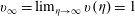
is chosen. It is assumed that each liquid is inviscid and incompressible, and gravity and surface tension effects can be neglected. A sketch of the problem shown in figure 1(a) includes the upper and lower liquid wedges, the interface separating them, and the definitions of the geometric parameters. At time
$Oxy$
is chosen. It is assumed that each liquid is inviscid and incompressible, and gravity and surface tension effects can be neglected. A sketch of the problem shown in figure 1(a) includes the upper and lower liquid wedges, the interface separating them, and the definitions of the geometric parameters. At time
 $t=0$
points
$t=0$
points
 $A(A^{\prime })$
and
$A(A^{\prime })$
and
 $O(O^{\prime })$
are the same, where the apexes of the impacting liquid wedges meet each other, and subsequently after the impact, point
$O(O^{\prime })$
are the same, where the apexes of the impacting liquid wedges meet each other, and subsequently after the impact, point
 $O(O^{\prime })$
moves away with a constant speed forming the line
$O(O^{\prime })$
moves away with a constant speed forming the line
 $OA(O^{\prime }A^{\prime })$
, whose shape has to be determined as a part of the solution of the problem. Without losing generality, point
$OA(O^{\prime }A^{\prime })$
, whose shape has to be determined as a part of the solution of the problem. Without losing generality, point
 $A(A^{\prime })$
after the impact can be assumed as the stagnation point (Semenov et al.
Reference Semenov, Wu and Oliver2013). This is because impact depends only on the relative velocity between the liquids and their individual velocities can be adjusted to meet this condition. Based on the illustration in figure 1(a), line
$A(A^{\prime })$
after the impact can be assumed as the stagnation point (Semenov et al.
Reference Semenov, Wu and Oliver2013). This is because impact depends only on the relative velocity between the liquids and their individual velocities can be adjusted to meet this condition. Based on the illustration in figure 1(a), line
 $O^{\prime }A^{\prime }$
is half of the interface of the two liquids while line
$O^{\prime }A^{\prime }$
is half of the interface of the two liquids while line
 $OA$
contains the interface and part of the surface
$OA$
contains the interface and part of the surface
 $OO^{\prime \prime }$
of the lower liquid. This can obviously be the other way round, or
$OO^{\prime \prime }$
of the lower liquid. This can obviously be the other way round, or
 $O$
is within
$O$
is within
 $O^{\prime \prime }A^{\prime }$
, which depends on the velocities, angles and the densities of the liquid wedges. At this stage we assume that the line
$O^{\prime \prime }A^{\prime }$
, which depends on the velocities, angles and the densities of the liquid wedges. At this stage we assume that the line
 $OA$
is an expanding surface, whose shape is given by the function
$OA$
is an expanding surface, whose shape is given by the function
 $Z_{\mathit{in}}(S,t)=X_{\mathit{in}}(S,t)+\text{i}Y_{\mathit{in}}(S,t)$
, where
$Z_{\mathit{in}}(S,t)=X_{\mathit{in}}(S,t)+\text{i}Y_{\mathit{in}}(S,t)$
, where
 $S$
is the arclength coordinate along the interface and
$S$
is the arclength coordinate along the interface and
 $t$
is time. This gives the possibility of decomposing the problem of impact between the two liquids into two similar problems of the impact of a lower/upper liquid wedge with the corresponding side of the expanding surface. We may use the lower liquid to demonstrate the solution procedure. For the impact of liquid wedges, both with constant velocity, the problem is self-similar since there is no length scale. As a result the time-dependent problem in the physical plane
$t$
is time. This gives the possibility of decomposing the problem of impact between the two liquids into two similar problems of the impact of a lower/upper liquid wedge with the corresponding side of the expanding surface. We may use the lower liquid to demonstrate the solution procedure. For the impact of liquid wedges, both with constant velocity, the problem is self-similar since there is no length scale. As a result the time-dependent problem in the physical plane
 $Z=X+\text{i}Y$
can be written in the stationary plane
$Z=X+\text{i}Y$
can be written in the stationary plane
 $z=x+\text{i}y$
in terms of the self-similar variables
$z=x+\text{i}y$
in terms of the self-similar variables
 $x=X/(Vt)$
,
$x=X/(Vt)$
,
 $y=Y/(Vt)$
where
$y=Y/(Vt)$
where
 $V$
is the magnitude of the incoming velocity of the lower liquid, or the velocity at infinity
$V$
is the magnitude of the incoming velocity of the lower liquid, or the velocity at infinity
 $BC$
in the physical plane. The complex velocity potential
$BC$
in the physical plane. The complex velocity potential
 $W(Z,t)={\it\Phi}(X,Y,t)+\text{i}{\it\Psi}(X,Y,t)$
of the lower liquid can be written in the form
$W(Z,t)={\it\Phi}(X,Y,t)+\text{i}{\it\Psi}(X,Y,t)$
of the lower liquid can be written in the form
 $$\begin{eqnarray}W(Z,t)=V^{2}tw(z).\end{eqnarray}$$
The problem becomes to determine the function
 $w(z)$
which conformally maps the stationary plane
$w(z)$
which conformally maps the stationary plane
 $z$
onto the complex-velocity potential region
$z$
onto the complex-velocity potential region
 $w$
. We choose the first quadrant of the
$w$
. We choose the first quadrant of the
 ${\it\zeta}$
-plane as the parameter region to derive expressions for the non-dimensional complex velocity,
${\it\zeta}$
-plane as the parameter region to derive expressions for the non-dimensional complex velocity,
 $\text{d}w/\text{d}z$
, and for the derivative of the complex potential,
$\text{d}w/\text{d}z$
, and for the derivative of the complex potential,
 $\text{d}w/\text{d}{\it\zeta}$
, both as functions of the variable
$\text{d}w/\text{d}{\it\zeta}$
, both as functions of the variable
 ${\it\zeta}$
. Once these functions are found, the velocity field and the relationship between the parameter region and the stationary plane
${\it\zeta}$
. Once these functions are found, the velocity field and the relationship between the parameter region and the stationary plane
 $z$
can be determined as follows:
$z$
can be determined as follows:
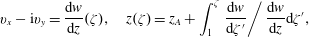 $$\begin{eqnarray}v_{x}-\text{i}v_{y}=\frac{\text{d}w}{\text{d}z}({\it\zeta}),\quad z({\it\zeta})=z_{A}+\int _{1}^{{\it\zeta}}\left.\frac{\text{d}w}{\text{d}{\it\zeta}^{\prime }}\right/\frac{\text{d}w}{\text{d}z}\text{d}{\it\zeta}^{\prime },\end{eqnarray}$$
where
 $v_{x}$
and
$v_{x}$
and
 $v_{y}$
are the
$v_{y}$
are the
 $x$
- and
$x$
- and
 $y$
-components of the velocity non-dimensionalized by
$y$
-components of the velocity non-dimensionalized by
 $V$
, and
$V$
, and
 $z_{A}=0$
is the origin.
$z_{A}=0$
is the origin.

Figure 1. Sketch of the collision of two liquid wedges: (a) the physical plane; (b) the parameter plane for the lower liquid; (c) the parameter plane for the upper liquid. (Points
 $O^{\prime }$
and
$O^{\prime }$
and
 $O^{\prime \prime }$
,
$O^{\prime \prime }$
,
 $B^{\prime }$
and
$B^{\prime }$
and
 $B^{\prime \prime }$
are symmetric respect to the
$B^{\prime \prime }$
are symmetric respect to the
 $Y$
-axis;
$Y$
-axis;
 $O^{\prime \prime }O$
is part of the free surface, but will be incorporated into the mathematical formulation for the interface when
$O^{\prime \prime }O$
is part of the free surface, but will be incorporated into the mathematical formulation for the interface when
 $O^{\prime \prime }$
is located within
$O^{\prime \prime }$
is located within
 $OA$
.)
$OA$
.)
Conformal mapping allows us to fix three arbitrary points in the parameter region, which are chosen as
 $O$
,
$O$
,
 $B$
and
$B$
and
 $A$
as shown in figure 1(b). Similarly, points
$A$
as shown in figure 1(b). Similarly, points
 $O^{\prime }$
,
$O^{\prime }$
,
 $B^{\prime }$
, and
$B^{\prime }$
, and
 $A^{\prime }$
are fixed in the parameter region
$A^{\prime }$
are fixed in the parameter region
 ${\it\zeta}^{\prime }$
shown in figure 1(c). In this plane, the positive part of the imaginary axis (
${\it\zeta}^{\prime }$
shown in figure 1(c). In this plane, the positive part of the imaginary axis (
 $0<{\it\eta}<\infty$
,
$0<{\it\eta}<\infty$
,
 ${\it\xi}=0$
) corresponds to the free surface
${\it\xi}=0$
) corresponds to the free surface
 $OB$
. The interval (
$OB$
. The interval (
 $0<{\it\xi}<1$
,
$0<{\it\xi}<1$
,
 ${\it\eta}=0$
) of the real axis corresponds to the surface
${\it\eta}=0$
) of the real axis corresponds to the surface
 $OA$
, and the rest of the positive real axis (
$OA$
, and the rest of the positive real axis (
 $1<{\it\xi}<\infty$
,
$1<{\it\xi}<\infty$
,
 ${\it\eta}=0$
) corresponds to the symmetry line
${\it\eta}=0$
) corresponds to the symmetry line
 $AC$
. We notice that
$AC$
. We notice that
 $OA$
may include both the interface
$OA$
may include both the interface
 $O^{\prime }A$
and the free surface
$O^{\prime }A$
and the free surface
 $OO^{\prime }$
. These two parts may both be included in the mathematical formulation for the interface below and
$OO^{\prime }$
. These two parts may both be included in the mathematical formulation for the interface below and
 $OA$
may be referred to as the interface during the derivation. However, the pressure continuity condition with the upper liquid will be imposed on
$OA$
may be referred to as the interface during the derivation. However, the pressure continuity condition with the upper liquid will be imposed on
 $AO^{\prime }$
(interface) and the constant pressure equal to the ambient pressure will be imposed on
$AO^{\prime }$
(interface) and the constant pressure equal to the ambient pressure will be imposed on
 $OO^{\prime }$
(free surface).
$OO^{\prime }$
(free surface).
2.1. Expressions for the complex velocity and for the derivative of the complex potential
The boundary-value problem for the complex velocity function can be formulated in the parameter plane as follows. At this stage we introduce function
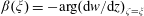 ${\it\beta}({\it\xi})=-\arg (\text{d}w/\text{d}z)_{{\it\zeta}={\it\xi}}$
along the interface, i.e. on the interval
${\it\beta}({\it\xi})=-\arg (\text{d}w/\text{d}z)_{{\it\zeta}={\it\xi}}$
along the interface, i.e. on the interval
 $0<{\it\xi}<1$
of the real axis of the parameter plane, and function
$0<{\it\xi}<1$
of the real axis of the parameter plane, and function
 $v({\it\eta})$
, which is the velocity modulus along the free surface or along the positive part of the imaginary axis of the
$v({\it\eta})$
, which is the velocity modulus along the free surface or along the positive part of the imaginary axis of the
 ${\it\zeta}$
-plane. This means that
${\it\zeta}$
-plane. This means that
 $$\begin{eqnarray}\displaystyle & \displaystyle {\it\chi}({\it\xi})=\arg (\text{d}w/\text{d}z)=\left\{\begin{array}{@{}l@{}}-{\it\beta}({\it\xi}),\quad 0<{\it\xi}<1,{\it\eta}=0,\\ -{\rm\pi}/2,\quad 1<{\it\xi}<\infty ,{\it\eta}=0.\end{array}\right. & \displaystyle\end{eqnarray}$$
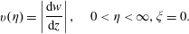 $$\begin{eqnarray}\displaystyle & \displaystyle v({\it\eta})=\left|\frac{\text{d}w}{\text{d}z}\right|,\quad 0<{\it\eta}<\infty ,{\it\xi}=0. & \displaystyle\end{eqnarray}$$
In the vicinity of stagnation point
 $A$
, or
$A$
, or
 $z=0$
, the leading term in
$z=0$
, the leading term in
 $w(z)-w_{A}$
will be
$w(z)-w_{A}$
will be
 $Dz^{2}$
as
$Dz^{2}$
as
 $\text{d}w/\text{d}z=0$
at the stagnation point. Here,
$\text{d}w/\text{d}z=0$
at the stagnation point. Here,
 $w_{A}=w(z)_{z=0}$
and the constant
$w_{A}=w(z)_{z=0}$
and the constant
 $D$
must be a real number as
$D$
must be a real number as
 $v_{x}=0$
on
$v_{x}=0$
on
 $x=0$
. Thus
$x=0$
. Thus
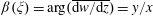 ${\it\beta}({\it\xi})=\arg (\overline{\text{d}w/\text{d}z})=y/x$
(
${\it\beta}({\it\xi})=\arg (\overline{\text{d}w/\text{d}z})=y/x$
(
 ${\it\xi}\rightarrow 1-{\it\varepsilon}$
,
${\it\xi}\rightarrow 1-{\it\varepsilon}$
,
 ${\it\varepsilon}\rightarrow 0$
). Since the problem is symmetric about
${\it\varepsilon}\rightarrow 0$
). Since the problem is symmetric about
 $x=0$
, the interface forms a right-angle with the
$x=0$
, the interface forms a right-angle with the
 $y$
-axis. As a result, the slope of the interface, which is
$y$
-axis. As a result, the slope of the interface, which is
 $\lim _{x\rightarrow \infty }\arg (\overline{\text{d}w/\text{d}z})=\lim _{x\rightarrow \infty }y/x$
at
$\lim _{x\rightarrow \infty }\arg (\overline{\text{d}w/\text{d}z})=\lim _{x\rightarrow \infty }y/x$
at
 $A$
, is zero. In other words
$A$
, is zero. In other words
 ${\it\beta}({\it\xi})_{{\it\xi}=1}=0$
. Thus, at point
${\it\beta}({\it\xi})_{{\it\xi}=1}=0$
. Thus, at point
 $A$
, the function
$A$
, the function
 ${\it\chi}({\it\xi})$
has a jump
${\it\chi}({\it\xi})$
has a jump
 ${\rm\Delta}{\it\chi}_{A}=-{\rm\pi}/2$
when
${\rm\Delta}{\it\chi}_{A}=-{\rm\pi}/2$
when
 ${\it\xi}$
increases from
${\it\xi}$
increases from
 $1-{\it\epsilon}$
to
$1-{\it\epsilon}$
to
 $1+{\it\epsilon}$
. The velocity magnitude at infinity at point
$1+{\it\epsilon}$
. The velocity magnitude at infinity at point
 $B$
,
$B$
,
 $v_{\infty }=\lim _{{\it\eta}\rightarrow \infty }v({\it\eta})=1$
, since
$v_{\infty }=\lim _{{\it\eta}\rightarrow \infty }v({\it\eta})=1$
, since
 $V$
is chosen as the reference velocity.
$V$
is chosen as the reference velocity.
The problem is then to find the function,
 $\text{d}w/\text{d}z$
, in the first quadrant of the parameter plane, which satisfies the boundary conditions in (2.3) and (2.4). It can be confirmed that these conditions are satisfied by the complex function
$\text{d}w/\text{d}z$
, in the first quadrant of the parameter plane, which satisfies the boundary conditions in (2.3) and (2.4). It can be confirmed that these conditions are satisfied by the complex function
 $F({\it\zeta})=\text{d}w/\text{d}z$
given in the following integral formula (Semenov & Cummings Reference Semenov and Cummings2006; Semenov & Iafrati Reference Semenov and Iafrati2006):
$F({\it\zeta})=\text{d}w/\text{d}z$
given in the following integral formula (Semenov & Cummings Reference Semenov and Cummings2006; Semenov & Iafrati Reference Semenov and Iafrati2006):
 $$\begin{eqnarray}F({\it\zeta})=v_{\infty }\exp \left[\frac{1}{{\rm\pi}}\int _{0}^{\infty }\frac{\text{d}{\it\chi}}{\text{d}{\it\xi}}\ln \left(\frac{{\it\zeta}+{\it\xi}}{{\it\zeta}-{\it\xi}}\right)\!\text{d}{\it\xi}-\frac{\text{i}}{{\rm\pi}}\int _{0}^{\infty }\frac{\text{d}\ln v}{\text{d}{\it\eta}}\ln \left(\frac{{\it\zeta}-\text{i}{\it\eta}}{{\it\zeta}+\text{i}{\it\eta}}\right)\!\text{d}{\it\eta}+\text{i}{\it\chi}_{\infty }\right],\end{eqnarray}$$
where
 ${\it\chi}({\it\xi})=\arg [F({\it\zeta})]_{{\it\zeta}={\it\xi}}$
and
${\it\chi}({\it\xi})=\arg [F({\it\zeta})]_{{\it\zeta}={\it\xi}}$
and
 $v({\it\eta})=|F({\it\zeta})|_{{\it\zeta}=\text{i}{\it\eta}}$
are the argument and magnitude of the function
$v({\it\eta})=|F({\it\zeta})|_{{\it\zeta}=\text{i}{\it\eta}}$
are the argument and magnitude of the function
 $F({\it\zeta})$
, respectively, with
$F({\it\zeta})$
, respectively, with
 ${\it\chi}_{\infty }={\it\chi}({\it\xi})_{{\it\xi}\rightarrow \infty }$
and
${\it\chi}_{\infty }={\it\chi}({\it\xi})_{{\it\xi}\rightarrow \infty }$
and
 $v_{\infty }=v({\it\eta})_{{\it\eta}\rightarrow \infty }$
.
$v_{\infty }=v({\it\eta})_{{\it\eta}\rightarrow \infty }$
.
Evaluating the first integral over
 $1<{\it\xi}<\infty$
with the second line of (2.3) and taking into account the step change in the function
$1<{\it\xi}<\infty$
with the second line of (2.3) and taking into account the step change in the function
 ${\it\chi}({\it\xi})$
at
${\it\chi}({\it\xi})$
at
 ${\it\xi}=1$
, we obtain an expression for the complex velocity in the
${\it\xi}=1$
, we obtain an expression for the complex velocity in the
 ${\it\zeta}$
-plane as
${\it\zeta}$
-plane as
 $$\begin{eqnarray}\frac{\text{d}w}{\text{d}z}=v_{0}\sqrt{\frac{1-{\it\zeta}}{1+{\it\zeta}}}\exp \left[\int _{0}^{1}\frac{\text{d}{\it\beta}}{\text{d}{\it\xi}}\ln \left(\frac{{\it\xi}-{\it\zeta}}{{\it\xi}+{\it\zeta}}\right)\!\text{d}{\it\xi}-\frac{\text{i}}{{\rm\pi}}\int _{0}^{\infty }\frac{\text{d}\ln v}{\text{d}{\it\eta}}\ln \left(\frac{\text{i}{\it\eta}-{\it\zeta}}{\text{i}{\it\eta}+{\it\zeta}}\right)\!\text{d}{\it\eta}-\text{i}{\it\beta}_{0}\right],\end{eqnarray}$$
where
 $$\begin{eqnarray}{\it\beta}_{0}={\it\beta}(1)+\int _{1}^{0}\frac{\text{d}{\it\beta}}{\text{d}{\it\xi}}\text{d}{\it\xi},\quad v_{0}=v_{\infty }\exp \left(\int _{\infty }^{0}\frac{\text{d}\ln v}{\text{d}{\it\eta}}\text{d}{\it\eta}\right)\end{eqnarray}$$
are the velocity direction and magnitude at point
 $O$
, respectively. In order to analyse the behaviour of the velocity potential along the entire flow boundary, it is useful to introduce the unit normal vector
$O$
, respectively. In order to analyse the behaviour of the velocity potential along the entire flow boundary, it is useful to introduce the unit normal vector
 $\boldsymbol{n}$
pointing out of the liquid region and the unit vector
$\boldsymbol{n}$
pointing out of the liquid region and the unit vector
 ${\bf\tau}$
obtained by rotating
${\bf\tau}$
obtained by rotating
 $\boldsymbol{n}$
by
$\boldsymbol{n}$
by
 ${\rm\pi}/2$
anticlockwise. Let
${\rm\pi}/2$
anticlockwise. Let
 $s$
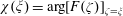
be the arclength coordinate along the boundary and when it increases the liquid region is on the left-hand side (see figure 1
a). With this notation, we can write
$s$
be the arclength coordinate along the boundary and when it increases the liquid region is on the left-hand side (see figure 1
a). With this notation, we can write
 $$\begin{eqnarray}\text{d}w=(v_{s}+\text{i}v_{n})\text{d}s=v\text{e}^{\text{i}{\it\omega}},\end{eqnarray}$$
where
 $v_{s}$
and
$v_{s}$
and
 $v_{n}$
are the tangential and normal velocity components along the flow boundary, respectively, and
$v_{n}$
are the tangential and normal velocity components along the flow boundary, respectively, and
 ${\it\omega}=\tan ^{-1}(v_{n}/v_{s})$
is angle between the velocity vector and vector
${\it\omega}=\tan ^{-1}(v_{n}/v_{s})$
is angle between the velocity vector and vector
 ${\bf\tau}$
on the flow boundary. In figure 2(a) is shown the variation of this angle along the boundary corresponding to the path along the axes of the first quadrant of figure 2(b) in the clockwise direction.
${\bf\tau}$
on the flow boundary. In figure 2(a) is shown the variation of this angle along the boundary corresponding to the path along the axes of the first quadrant of figure 2(b) in the clockwise direction.

Figure 2. (a) Behaviour of the velocity angle
 ${\it\omega}=\tan ^{-1}(v_{n}/v_{s})$
to the flow boundary. The solid lines correspond to the continuous changes in the function
${\it\omega}=\tan ^{-1}(v_{n}/v_{s})$
to the flow boundary. The solid lines correspond to the continuous changes in the function
 ${\it\omega}({\it\zeta})$
while the step changes are shown by the dashed lines. (b) The corresponding variation of the variable
${\it\omega}({\it\zeta})$
while the step changes are shown by the dashed lines. (b) The corresponding variation of the variable
 ${\it\zeta}$
in the parameter region.
${\it\zeta}$
in the parameter region.
Now we introduce the functions
 ${\it\theta}({\it\eta})={\it\omega}({\it\zeta})_{{\it\zeta}=\text{i}{\it\eta}}$
and
${\it\theta}({\it\eta})={\it\omega}({\it\zeta})_{{\it\zeta}=\text{i}{\it\eta}}$
and
 ${\it\gamma}({\it\xi})={\it\omega}({\it\zeta})_{{\it\zeta}={\it\xi}}$
along the positive parts of the imaginary and real axes of the
${\it\gamma}({\it\xi})={\it\omega}({\it\zeta})_{{\it\zeta}={\it\xi}}$
along the positive parts of the imaginary and real axes of the
 ${\it\zeta}$
-plane, respectively. Between points
${\it\zeta}$
-plane, respectively. Between points
 $C$
and
$C$
and
 $A$
, or
$A$
, or
 $1<{\it\xi}<\infty$
, function
$1<{\it\xi}<\infty$
, function
 ${\it\gamma}=-{\rm\pi}$
, since
${\it\gamma}=-{\rm\pi}$
, since
 $v_{n}=0$
and
$v_{n}=0$
and
 $v_{s}<0$
according to the direction of the vector
$v_{s}<0$
according to the direction of the vector
 ${\bf\tau}$
. When moving from point
${\bf\tau}$
. When moving from point
 $A$
to point
$A$
to point
 $O_{-}$
along the interface, the function
$O_{-}$
along the interface, the function
 ${\it\gamma}({\it\xi})$
changes continuously from value
${\it\gamma}({\it\xi})$
changes continuously from value
 ${\it\gamma}_{A}=-{\rm\pi}$
to some value
${\it\gamma}_{A}=-{\rm\pi}$
to some value
 ${\it\gamma}_{0}={\it\gamma}({\it\xi})_{{\it\xi}=0}$
at point
${\it\gamma}_{0}={\it\gamma}({\it\xi})_{{\it\xi}=0}$
at point
 $O_{-}$
. When we move in the counterclockwise direction along an infinitesimal quarter of circle centred at the point
$O_{-}$
. When we move in the counterclockwise direction along an infinitesimal quarter of circle centred at the point
 ${\it\zeta}=0$
in the parameter plane the corresponding line in the physical plane moves to the vicinity of the tip. The jump in the function
${\it\zeta}=0$
in the parameter plane the corresponding line in the physical plane moves to the vicinity of the tip. The jump in the function
 ${\it\gamma}({\it\xi})$
equals
${\it\gamma}({\it\xi})$
equals
 ${\rm\Delta}_{O}={\it\theta}_{0}-{\it\gamma}_{0}$
, where
${\rm\Delta}_{O}={\it\theta}_{0}-{\it\gamma}_{0}$
, where
 ${\it\theta}_{0}={\it\theta}({\it\eta})_{{\it\eta}=0}$
and
${\it\theta}_{0}={\it\theta}({\it\eta})_{{\it\eta}=0}$
and
 ${\it\gamma}_{0}={\it\gamma}({\it\xi})_{{\it\xi}=0}$
. Hence, the contact angle between the free surface
${\it\gamma}_{0}={\it\gamma}({\it\xi})_{{\it\xi}=0}$
. Hence, the contact angle between the free surface
 $BO$
and the interface
$BO$
and the interface
 $O^{\prime }O$
(also a free surface in the physical plane for the reason in the paragraph above § 2.1) at point
$O^{\prime }O$
(also a free surface in the physical plane for the reason in the paragraph above § 2.1) at point
 $O$
is
$O$
is
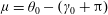 ${\it\mu}={\it\theta}_{0}-({\it\gamma}_{0}+{\rm\pi})$
, as can be seen from figure 2(a). Based on the above considerations we can write the function
${\it\mu}={\it\theta}_{0}-({\it\gamma}_{0}+{\rm\pi})$
, as can be seen from figure 2(a). Based on the above considerations we can write the function
 ${\it\omega}({\it\zeta})$
as follows:
${\it\omega}({\it\zeta})$
as follows:
 $$\begin{eqnarray}{\it\omega}({\it\zeta})=\arg \left(\frac{\text{d}w}{\text{d}s}\right)=\left\{\begin{array}{@{}ll@{}}{\it\gamma}({\it\xi}), & 0<{\it\xi}<1,{\it\eta}=0,\\ {\it\gamma}_{0}+{\it\theta}({\it\eta})-{\it\theta}_{0}+{\rm\Delta}_{O}, & {\it\xi}=0,0<{\it\eta}<\infty .\end{array}\right.\end{eqnarray}$$
Equation (2.8) allows us to determine the argument of the derivative of the complex potential
 $$\begin{eqnarray}\displaystyle {\it\vartheta}({\it\zeta}) & = & \displaystyle \arg \left(\frac{\text{d}w}{\text{d}{\it\zeta}}\right)=\arg \left(\frac{\text{d}w}{\text{d}s}\right)+\arg \left(\frac{\text{d}s}{\text{d}{\it\zeta}}\right)={\it\omega}({\it\zeta})+\left\{\begin{array}{@{}ll@{}}0, & 0<{\it\xi}<1,{\it\eta}=0,\\ {\rm\pi}/2, & {\it\xi}=0,0<{\it\eta}<\infty \end{array}\right.\nonumber\\ \displaystyle & = & \displaystyle \left\{\begin{array}{@{}ll@{}}{\it\gamma}({\it\xi}), & 0<{\it\xi}<1,{\it\eta}=0,\\ {\it\gamma}_{0}+{\it\theta}({\it\eta})-{\it\theta}_{0}+{\rm\Delta}_{{\it\vartheta}}, & {\it\xi}=0,0<{\it\eta}<\infty ,\end{array}\right.\end{eqnarray}$$
where
 ${\rm\Delta}_{{\it\vartheta}}={\rm\Delta}_{O}+{\rm\pi}/2={\it\mu}-{\rm\pi}/2$
is the jump in the function
${\rm\Delta}_{{\it\vartheta}}={\rm\Delta}_{O}+{\rm\pi}/2={\it\mu}-{\rm\pi}/2$
is the jump in the function
 ${\it\vartheta}({\it\zeta})$
when it passes point
${\it\vartheta}({\it\zeta})$
when it passes point
 $O$
(
$O$
(
 ${\it\zeta}=0$
) in the parameter region along an infinitesimal quarter circle centred at
${\it\zeta}=0$
) in the parameter region along an infinitesimal quarter circle centred at
 ${\it\zeta}=0$
. The corresponding change of the argument
${\it\zeta}=0$
. The corresponding change of the argument
 $\arg {\it\zeta}$
equals
$\arg {\it\zeta}$
equals
 ${\rm\pi}/2$
, and so we can expect that function
${\rm\pi}/2$
, and so we can expect that function
 $\text{d}w/\text{d}{\it\zeta}$
at point
$\text{d}w/\text{d}{\it\zeta}$
at point
 $O$
has singularity of order
$O$
has singularity of order
 $\text{d}w/\text{d}{\it\zeta}\sim {\it\zeta}^{2{\rm\Delta}_{{\it\vartheta}}/{\rm\pi}}$
.
$\text{d}w/\text{d}{\it\zeta}\sim {\it\zeta}^{2{\rm\Delta}_{{\it\vartheta}}/{\rm\pi}}$
.
The problem is then to find a complex function
 $G({\it\zeta})=\text{d}w/\text{d}{\it\zeta}$
in the first quadrant of the parameter plane which satisfies the boundary conditions (2.10). This is a uniform boundary-value problem, or a problem that has the same type of boundary conditions on the real and imaginary axes of the first quadrant of the parameter plane. Using the integral formula (Semenov & Cummings Reference Semenov and Cummings2006; Semenov & Iafrati Reference Semenov and Iafrati2006), we have
$G({\it\zeta})=\text{d}w/\text{d}{\it\zeta}$
in the first quadrant of the parameter plane which satisfies the boundary conditions (2.10). This is a uniform boundary-value problem, or a problem that has the same type of boundary conditions on the real and imaginary axes of the first quadrant of the parameter plane. Using the integral formula (Semenov & Cummings Reference Semenov and Cummings2006; Semenov & Iafrati Reference Semenov and Iafrati2006), we have
 $$\begin{eqnarray}G({\it\zeta})=K\exp \left[\frac{1}{{\rm\pi}}\int _{\infty }^{0}\frac{\text{d}{\it\vartheta}}{\text{d}{\it\xi}}\ln ({\it\zeta}^{2}-{\it\xi}^{2})\text{d}{\it\xi}+\frac{1}{{\rm\pi}}\int _{0}^{\infty }\frac{\text{d}{\it\vartheta}}{\text{d}{\it\eta}}\ln ({\it\zeta}^{2}+{\it\eta}^{2})\text{d}{\it\eta}+\text{i}{\it\vartheta}_{\infty }\right],\end{eqnarray}$$
where
 $K$
is a real factor,
$K$
is a real factor,
 ${\it\vartheta}({\it\zeta})=\arg [G({\it\vartheta})]$
,
${\it\vartheta}({\it\zeta})=\arg [G({\it\vartheta})]$
,
 $0<{\it\xi}<\infty$
,
$0<{\it\xi}<\infty$
,
 ${\it\eta}=0$
and
${\it\eta}=0$
and
 $0<{\it\eta}<\infty$
,
$0<{\it\eta}<\infty$
,
 ${\it\xi}=0$
,
${\it\xi}=0$
,
 ${\it\vartheta}_{\infty }={\it\vartheta}({\it\zeta})_{|{\it\zeta}|\rightarrow \infty }$
. We evaluate the integrals over each step change of the function
${\it\vartheta}_{\infty }={\it\vartheta}({\it\zeta})_{|{\it\zeta}|\rightarrow \infty }$
. We evaluate the integrals over each step change of the function
 ${\it\vartheta}({\it\zeta})$
, and finally obtain an expression for the derivative of the complex potential in the
${\it\vartheta}({\it\zeta})$
, and finally obtain an expression for the derivative of the complex potential in the
 ${\it\zeta}$
-plane as
${\it\zeta}$
-plane as
 $$\begin{eqnarray}\frac{\text{d}w}{\text{d}{\it\zeta}}=K{\it\zeta}^{2{\it\mu}/{\rm\pi}-1}\exp \left[-\frac{1}{{\rm\pi}}\int _{0}^{1}\frac{\text{d}{\it\gamma}}{\text{d}{\it\xi}}\ln ({\it\xi}^{2}-{\it\zeta}^{2})\text{d}{\it\xi}+\frac{1}{{\rm\pi}}\int _{0}^{\infty }\frac{\text{d}{\it\theta}}{\text{d}{\it\eta}}\ln ({\it\zeta}^{2}+{\it\eta}^{2})\text{d}{\it\eta}\right].\end{eqnarray}$$
Integration of (2.12) in the parameter region allows us to obtain the function
 $w({\it\zeta})$
which conformally maps the parameter region onto the corresponding region in the complex-potential plane:
$w({\it\zeta})$
which conformally maps the parameter region onto the corresponding region in the complex-potential plane:
 $$\begin{eqnarray}\displaystyle w({\it\zeta}) & = & \displaystyle w_{A}+K\int _{1}^{{\it\zeta}}{\it\zeta}^{\prime (2{\it\mu}/{\rm\pi}-1)}\nonumber\\ \displaystyle & & \displaystyle \times \exp \left[-\frac{1}{{\rm\pi}}\int _{0}^{1}\frac{\text{d}{\it\gamma}}{\text{d}{\it\xi}}\ln ({\it\xi}^{2}-{\it\zeta}^{\prime 2})\text{d}{\it\xi}+\frac{1}{{\rm\pi}}\int _{0}^{\infty }\frac{\text{d}{\it\theta}}{\text{d}{\it\eta}}\ln ({\it\zeta}^{\prime 2}+{\it\eta}^{2})\text{d}{\it\eta}\right]\!\text{d}{\it\zeta}^{\prime },\end{eqnarray}$$
where
 $w_{A}$
is the complex potential at point
$w_{A}$
is the complex potential at point
 $A$
. As an arbitrary constant can be included when integration is applied to (2.12), without losing generality we can choose
$A$
. As an arbitrary constant can be included when integration is applied to (2.12), without losing generality we can choose
 $w_{A}=0$
.
$w_{A}=0$
.
Dividing (2.12) by (2.6), we can obtain the derivative of the mapping function between fluid domains in the similarity plane,
 $z$
, and the parameter plane,
$z$
, and the parameter plane,
 ${\it\zeta}$
:
${\it\zeta}$
:
 $$\begin{eqnarray}\displaystyle \frac{\text{d}z}{\text{d}{\it\zeta}} & = & \displaystyle \frac{K}{v_{0}}{\it\zeta}^{2{\it\mu}/{\rm\pi}-1}\sqrt{\frac{1+{\it\zeta}}{1-{\it\zeta}}}\exp \left[-\frac{1}{{\rm\pi}}\int _{0}^{1}\frac{\text{d}{\it\gamma}}{\text{d}{\it\xi}}\ln ({\it\xi}^{2}-{\it\zeta}^{2})\text{d}{\it\xi}+\frac{1}{{\rm\pi}}\int _{0}^{\infty }\frac{\text{d}{\it\theta}}{\text{d}{\it\eta}}\ln ({\it\eta}^{2}+{\it\zeta}^{2})\text{d}{\it\eta}\right.\nonumber\\ \displaystyle & & \displaystyle -\left.\frac{1}{{\rm\pi}}\int _{0}^{1}\frac{\text{d}{\it\beta}}{\text{d}{\it\xi}}\ln \left(\frac{{\it\xi}-{\it\zeta}}{{\it\xi}+{\it\zeta}}\right)\!\text{d}{\it\xi}+\frac{\text{i}}{{\rm\pi}}\int _{0}^{\infty }\frac{\text{d}\ln v}{\text{d}{\it\eta}}\ln \left(\frac{{\it\eta}-{\it\zeta}}{{\it\eta}+{\it\zeta}}\right)\!\text{d}{\it\eta}+\text{i}{\it\beta}_{0}\right].\end{eqnarray}$$
The integration of this equation can give the mapping function
 $z=z({\it\zeta})$
. Equations (2.6), (2.12) and (2.14) include the parameter
$z=z({\it\zeta})$
. Equations (2.6), (2.12) and (2.14) include the parameter
 $K$
and the functions
$K$
and the functions
 ${\it\gamma}({\it\xi})$
,
${\it\gamma}({\it\xi})$
,
 ${\it\beta}({\it\xi})$
,
${\it\beta}({\it\xi})$
,
 ${\it\theta}({\it\eta})$
and
${\it\theta}({\it\eta})$
and
 $v({\it\eta})$
, all to be determined from physical considerations, as well as the dynamic and kinematic boundary conditions on the free surface and the interface.
$v({\it\eta})$
, all to be determined from physical considerations, as well as the dynamic and kinematic boundary conditions on the free surface and the interface.
The fluid particle at point
 $O$
was at point
$O$
was at point
 $A$
at the moment when the tips of the wedges touch each other. In the physical plane, the position of point
$A$
at the moment when the tips of the wedges touch each other. In the physical plane, the position of point
 $O$
can then be linked to the particle velocity, which is a constant
$O$
can then be linked to the particle velocity, which is a constant
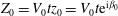 $Z_{0}=V_{0}tz_{0}=V_{0}t\text{e}^{\text{i}{\it\beta}_{0}}$
. Thus, the length of the interface
$Z_{0}=V_{0}tz_{0}=V_{0}t\text{e}^{\text{i}{\it\beta}_{0}}$
. Thus, the length of the interface
 $OA$
,
$OA$
,
 $s_{OA}$
, in the similarity plane, and the parameter
$s_{OA}$
, in the similarity plane, and the parameter
 $K$
can be determined, respectively, from the following equations:
$K$
can be determined, respectively, from the following equations:
 $$\begin{eqnarray}\displaystyle & \displaystyle \int _{0}^{s_{OA}}\text{e}^{\text{i}{\it\delta}(s)}\text{d}s=z_{0}=v_{0}\text{e}^{\text{i}{\it\beta}_{0}}, & \displaystyle\end{eqnarray}$$
 $$\begin{eqnarray}\displaystyle & \displaystyle K\int _{0}^{1}\frac{1}{K}\frac{\text{d}s}{\text{d}{\it\xi}}\text{d}{\it\xi}=s_{OA}, & \displaystyle\end{eqnarray}$$
when the functions
 ${\it\gamma}({\it\xi})$
,
${\it\gamma}({\it\xi})$
,
 ${\it\beta}({\it\xi})$
,
${\it\beta}({\it\xi})$
,
 ${\it\theta}({\it\eta})$
and
${\it\theta}({\it\eta})$
and
 $v({\it\eta})$
have been found. Here, the derivative
$v({\it\eta})$
have been found. Here, the derivative
 $$\begin{eqnarray}\frac{\text{d}s}{\text{d}{\it\xi}}=\left|\frac{\text{d}z}{\text{d}{\it\zeta}}\right|_{{\it\zeta}={\it\xi}}\end{eqnarray}$$
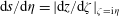
is obtained from (2.14), and
 ${\it\delta}$
is the slope of the interface as a function of the spatial coordinate
${\it\delta}$
is the slope of the interface as a function of the spatial coordinate
 $s$
.
$s$
.
The integral formulae (2.5) and (2.11) have enabled us to find expressions for the complex velocity and for the derivative of the complex potential defined in the parameter plane, and to extract all the flow singularities in an explicit form. These expressions contain unknown non-singular functions, namely the velocity magnitude,
 $v({\it\eta})$
, and direction,
$v({\it\eta})$
, and direction,
 ${\it\beta}({\it\xi})$
, as well as angle of the velocity to the flow boundary on the interface,
${\it\beta}({\it\xi})$
, as well as angle of the velocity to the flow boundary on the interface,
 ${\it\gamma}({\it\xi})$
, and free surface,
${\it\gamma}({\it\xi})$
, and free surface,
 ${\it\theta}({\it\eta})$
, which are determined from dynamic and kinematic boundary conditions.
${\it\theta}({\it\eta})$
, which are determined from dynamic and kinematic boundary conditions.
2.2. Dynamic and kinematic boundary conditions
The dynamic condition on the free surface requires
 $P=P_{a}$
, where
$P=P_{a}$
, where
 $P_{a}$
is ambient pressure. Using the Bernoulli equation and the property of self-similar flow for the temporal derivative of the potential, Semenov & Iafrati (Reference Semenov and Iafrati2006) obtained the dynamic boundary condition in the following form:
$P_{a}$
is ambient pressure. Using the Bernoulli equation and the property of self-similar flow for the temporal derivative of the potential, Semenov & Iafrati (Reference Semenov and Iafrati2006) obtained the dynamic boundary condition in the following form:
 $$\begin{eqnarray}\frac{\text{d}{\it\theta}}{\text{d}s}=\frac{v+s\cos {\it\theta}}{s\sin {\it\theta}}\frac{\text{d}\ln v}{\text{d}s}.\end{eqnarray}$$
Based on the momentum equation, the dynamic condition
 $P=P_{a}$
is also equivalent to the acceleration of the fluid particle on the free surface being orthogonal to the free surface. Combining this with the fact that the fluid particle on the free surface remains on the free surface, Semenov & Iafrati (Reference Semenov and Iafrati2006) further obtained the following equation:
$P=P_{a}$
is also equivalent to the acceleration of the fluid particle on the free surface being orthogonal to the free surface. Combining this with the fact that the fluid particle on the free surface remains on the free surface, Semenov & Iafrati (Reference Semenov and Iafrati2006) further obtained the following equation:
 $$\begin{eqnarray}\frac{1}{\tan {\it\theta}}\frac{\text{d}\ln v}{\text{d}s}=\frac{\text{d}}{\text{d}s}\left[\arg \left(\frac{\text{d}w}{\text{d}z}\right)\right]\end{eqnarray}$$
for the self-similar flow.
Multiplying both sides of (2.18) and (2.19) by
 $\text{d}s/\text{d}{\it\eta}=|\text{d}z/\text{d}{\it\zeta}|_{{\it\zeta}=\text{i}{\it\eta}}$
we obtain the following integro-differential equation for the function
$\text{d}s/\text{d}{\it\eta}=|\text{d}z/\text{d}{\it\zeta}|_{{\it\zeta}=\text{i}{\it\eta}}$
we obtain the following integro-differential equation for the function
 ${\it\theta}$
:
${\it\theta}$
:
 $$\begin{eqnarray}\frac{\text{d}{\it\theta}}{\text{d}{\it\eta}}=\frac{v+s\cos {\it\theta}}{s\sin {\it\theta}}\frac{\text{d}\ln v}{\text{d}{\it\eta}},\end{eqnarray}$$
where
 $s=s({\it\eta})$
is obtained by integration of the expression
$s=s({\it\eta})$
is obtained by integration of the expression
 $\text{d}s/\text{d}{\it\eta}=|\text{d}z/\text{d}{\it\zeta}|_{{\it\zeta}=\text{i}{\it\eta}}$
along the imaginary axis of the parameter plane:
$\text{d}s/\text{d}{\it\eta}=|\text{d}z/\text{d}{\it\zeta}|_{{\it\zeta}=\text{i}{\it\eta}}$
along the imaginary axis of the parameter plane:
 $$\begin{eqnarray}\displaystyle s({\it\eta})=-K\int _{0}^{{\it\eta}}\frac{{\it\zeta}^{2{\it\mu}/{\rm\pi}-1}}{v({\it\eta})}\exp \left[-\frac{1}{{\rm\pi}}\int _{0}^{1}\frac{\text{d}{\it\gamma}}{\text{d}{\it\xi}}\ln ({\it\xi}^{2}+{\it\eta}^{2})\text{d}{\it\xi}+\frac{1}{{\rm\pi}}\int _{0}^{\infty }\frac{\text{d}{\it\theta}}{\text{d}{\it\eta}^{\prime }}\ln ({{\it\eta}^{\prime }}^{2}-{\it\eta}^{2})\text{d}{\it\eta}^{\prime }\right]. & & \displaystyle \nonumber\\ \displaystyle & & \displaystyle\end{eqnarray}$$
By writing (2.6) for
 ${\it\zeta}=\text{i}{\it\eta}$
, the argument of the complex velocity along the free surface is obtained as
${\it\zeta}=\text{i}{\it\eta}$
, the argument of the complex velocity along the free surface is obtained as
 $$\begin{eqnarray}\displaystyle \arg \left(\frac{\text{d}w}{\text{d}z}\right)_{{\it\zeta}=\text{i}{\it\eta}} & = & \displaystyle \text{Im}\left\{\ln \left(\frac{\text{d}w}{\text{d}z}\right)_{{\it\zeta}=\text{i}{\it\eta}}\right\}\nonumber\\ \displaystyle & = & \displaystyle -\tan ^{-1}{\it\eta}-\frac{2}{{\rm\pi}}\int _{0}^{1}\frac{\text{d}{\it\beta}}{\text{d}{\it\xi}}\tan \frac{{\it\eta}}{{\it\xi}}\text{d}{\it\xi}-\frac{1}{{\rm\pi}}\int _{0}^{\infty }\frac{\text{d}\ln v}{\text{d}{\it\eta}^{\prime }}\ln \left|\frac{{\it\eta}^{\prime }-{\it\eta}}{{\it\eta}^{\prime }+{\it\eta}}\right|\!\text{d}{\it\eta}^{\prime }-{\it\beta}_{0}.\nonumber\\ \displaystyle & & \displaystyle\end{eqnarray}$$
Differentiating the above equation with respect to
 ${\it\eta}$
and substituting the result into (2.19), the following integral equation for the function
${\it\eta}$
and substituting the result into (2.19), the following integral equation for the function
 $\text{d}\ln v/\text{d}{\it\eta}$
is obtained:
$\text{d}\ln v/\text{d}{\it\eta}$
is obtained:
 $$\begin{eqnarray}-\frac{1}{\tan {\it\theta}}\frac{\text{d}\ln v}{\text{d}{\it\eta}}+\frac{1}{{\rm\pi}}\int _{0}^{\infty }\frac{\text{d}\ln v}{\text{d}{\it\eta}^{\prime }}\frac{2{\it\eta}^{\prime }}{{\it\eta}^{\prime 2}-{\it\eta}^{2}}\text{d}{\it\eta}^{\prime }=\frac{1}{1+{\it\eta}^{2}}+\frac{1}{{\rm\pi}}\int _{0}^{\infty }\frac{\text{d}{\it\beta}}{\text{d}{\it\xi}}\frac{2{\it\xi}}{{\it\xi}^{2}+{\it\eta}^{2}}\text{d}{\it\xi}.\end{eqnarray}$$
The system of equations (2.20) and (2.23) enables us to determine the functions
 ${\it\theta}({\it\eta})$
and
${\it\theta}({\it\eta})$
and
 $\text{d}\ln v/\text{d}{\it\eta}$
along the imaginary axis of the parameter domain. Then, the velocity magnitude on the free surface can be obtained from
$\text{d}\ln v/\text{d}{\it\eta}$
along the imaginary axis of the parameter domain. Then, the velocity magnitude on the free surface can be obtained from
 $$\begin{eqnarray}\displaystyle v({\it\eta})=v_{\infty }\exp \left(-\int _{{\it\eta}}^{\infty }\frac{\text{d}\ln v}{\text{d}{\it\eta}^{\prime }}\text{d}{\it\eta}^{\prime }\right), & & \displaystyle\end{eqnarray}$$
where
 $v_{\infty }$
is the given velocity at infinity. This gives the velocity at point
$v_{\infty }$
is the given velocity at infinity. This gives the velocity at point
 $O$
,
$O$
,
 $v_{0}=v({\it\eta})_{{\it\eta}=0}$
.
$v_{0}=v({\it\eta})_{{\it\eta}=0}$
.
The normal component of the velocity on the interface can be determined by exploiting the fact that the interface
 $Z_{\mathit{in}}=Z_{\mathit{in}}(S)=X_{\mathit{in}}(S)+\text{i}Y_{\mathit{in}}(S)$
is an expanding self-similar surface. By using the self-similar variable
$Z_{\mathit{in}}=Z_{\mathit{in}}(S)=X_{\mathit{in}}(S)+\text{i}Y_{\mathit{in}}(S)$
is an expanding self-similar surface. By using the self-similar variable
 $z=Z/(Vt)$
we can write
$z=Z/(Vt)$
we can write
 $Z_{\mathit{in}}=Vtz_{\mathit{in}}$
, and the slope of the interface
$Z_{\mathit{in}}=Vtz_{\mathit{in}}$
, and the slope of the interface
 ${\it\delta}_{\mathit{in}}(S)={\it\delta}_{\mathit{in}}(s)=\arg (\text{d}z_{\mathit{in}}/\text{d}s)$
. With the notation in (2.8) and using
${\it\delta}_{\mathit{in}}(S)={\it\delta}_{\mathit{in}}(s)=\arg (\text{d}z_{\mathit{in}}/\text{d}s)$
. With the notation in (2.8) and using
 $\text{d}s/\text{d}t|_{S}=-s/t$
, we obtain
$\text{d}s/\text{d}t|_{S}=-s/t$
, we obtain
 $$\begin{eqnarray}\text{d}W=V^{2}t\text{d}w=V^{2}t(v_{s}+\text{i}v_{n})\text{d}s=\frac{\text{d}\overline{Z}_{\mathit{in}}}{\text{d}t}\text{d}Z=Vt\frac{\text{d}\overline{Z}_{\mathit{in}}}{\text{d}t}\frac{\text{d}\overline{z}_{\mathit{in}}}{\text{d}s}\text{d}s=V^{2}t(\overline{z}_{\mathit{in}}-\text{e}^{-\text{i}{\it\delta}_{\mathit{in}}}s)\text{e}^{\text{i}{\it\delta}_{\mathit{in}}}\text{d}s,\end{eqnarray}$$
from which the normal component of the velocity on the interface is obtained as
 $$\begin{eqnarray}v_{n}=\text{Im}(\overline{z}_{\mathit{in}}(s)\text{e}^{\text{i}{\it\delta}_{\mathit{in}}(s)}).\end{eqnarray}$$
The tangential component of the velocity on the interface can be determined with the notation in (2.8):
 $$\begin{eqnarray}v_{s}=\text{Re}\left(\frac{\text{d}w}{\text{d}z}\frac{\text{d}z}{\text{d}s}\right)=\text{Re}\left(\left.\frac{\text{d}w}{\text{d}z}\right|_{{\it\zeta}={\it\xi}}\text{e}^{\text{i}{\it\delta}_{\mathit{in}}[s({\it\xi})]}\right),\end{eqnarray}$$
where
 $$\begin{eqnarray}s({\it\xi})=\int _{1}^{{\it\xi}}\frac{\text{d}s}{\text{d}{\it\xi}^{\prime }}\text{d}{\it\xi}^{\prime }\end{eqnarray}$$
is the spatial coordinate along the interface with its origin at point
 $A$
, and
$A$
, and
 $\text{d}s/\text{d}{\it\xi}^{\prime }$
is given in (2.17).
$\text{d}s/\text{d}{\it\xi}^{\prime }$
is given in (2.17).
By using (2.26), (2.27) and the definition of the function
 ${\it\gamma}({\it\xi})$
we can obtain
${\it\gamma}({\it\xi})$
we can obtain
 $$\begin{eqnarray}{\it\gamma}({\it\xi})=\tan ^{-1}\left(\frac{\text{Im}\{\overline{z}_{\mathit{in}}[s({\it\xi})]\text{e}^{\text{i}{\it\delta}_{\mathit{in}}[s({\it\xi})]}\}}{\text{Re}\{\text{d}w/\text{d}z|_{{\it\zeta}={\it\xi}}\text{e}^{\text{i}{\it\delta}_{\mathit{in}}[s({\it\xi})]}\}}\right).\end{eqnarray}$$
The angle
 ${\it\delta}_{\mathit{in}}$
between the unit vector
${\it\delta}_{\mathit{in}}$
between the unit vector
 ${\bf\tau}$
on the interface and the
${\bf\tau}$
on the interface and the
 $x$
-axis determined by the given shape of the interface can be expressed through the angles
$x$
-axis determined by the given shape of the interface can be expressed through the angles
 ${\it\beta}$
and
${\it\beta}$
and
 ${\it\gamma}$
. Taking the argument of (2.14) as
${\it\gamma}$
. Taking the argument of (2.14) as
 ${\it\delta}_{\mathit{in}}={\it\beta}+{\it\gamma}$
, the function
${\it\delta}_{\mathit{in}}={\it\beta}+{\it\gamma}$
, the function
 ${\it\beta}({\it\xi})$
is obtained as
${\it\beta}({\it\xi})$
is obtained as
 $$\begin{eqnarray}{\it\beta}({\it\xi})={\it\delta}_{\mathit{in}}[s({\it\xi})]-{\it\gamma}({\it\xi}).\end{eqnarray}$$
The system of integral equations (2.20), (2.23) allows us to determine the functions
 ${\it\theta}({\it\eta})$
and
${\it\theta}({\it\eta})$
and
 $v({\it\eta})$
together with the functions
$v({\it\eta})$
together with the functions
 ${\it\gamma}({\it\xi})$
and
${\it\gamma}({\it\xi})$
and
 ${\it\beta}({\it\xi})$
using (2.29) and (2.30). Once these functions are found, the angle of the tip
${\it\beta}({\it\xi})$
using (2.29) and (2.30). Once these functions are found, the angle of the tip
 $O$
,
$O$
,
 ${\it\mu}={\it\theta}({\it\eta})_{{\it\eta}=0}-{\it\gamma}({\it\xi})_{{\it\xi}=0}-{\rm\pi}$
(see figure 2
a) can be obtained.
${\it\mu}={\it\theta}({\it\eta})_{{\it\eta}=0}-{\it\gamma}({\it\xi})_{{\it\xi}=0}-{\rm\pi}$
(see figure 2
a) can be obtained.
By choosing the location of the reference point in the Bernoulli equation at the stagnation point
 $A$
and taking advantage of the self-similarity of the flow, we can determine the pressure coefficient at any point of the flow region by using
$A$
and taking advantage of the self-similarity of the flow, we can determine the pressure coefficient at any point of the flow region by using
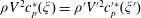
 $$\begin{eqnarray}c_{p}^{\ast }=\frac{2(P-P_{A})}{{\it\rho}V^{2}}=\text{Re}\left(-2w+2z\frac{\text{d}w}{\text{d}z}\right)-\left|\frac{\text{d}w}{\text{d}z}\right|^{2},\end{eqnarray}$$
in which
 $w_{A}=0$
, discussed after (2.13), has been used. Then, the pressure coefficient based on the ambient pressure,
$w_{A}=0$
, discussed after (2.13), has been used. Then, the pressure coefficient based on the ambient pressure,
 $P_{a}$
, is determined as follows:
$P_{a}$
, is determined as follows:
 $$\begin{eqnarray}c_{p}({\it\xi})=\frac{2(P-P_{a})}{{\it\rho}V^{2}}=c_{p}^{\ast }({\it\xi})-c_{p}^{\ast }(0).\end{eqnarray}$$
2.3. Iteration procedure to determine the shape of the interface
The problems will be solved alternately for lower and upper liquids. Once the incoming speed
 $V$
of the lower liquid wedge is chosen as the reference velocity, the incoming velocity
$V$
of the lower liquid wedge is chosen as the reference velocity, the incoming velocity
 $V^{\prime }$
of the upper liquid wedge can be obtained by equating the pressures
$V^{\prime }$
of the upper liquid wedge can be obtained by equating the pressures
 $P$
and
$P$
and
 $P^{\prime }$
at point
$P^{\prime }$
at point
 $A$
. From (2.32), we have
$A$
. From (2.32), we have
 $$\begin{eqnarray}V^{\prime }=V\sqrt{\frac{{\it\rho}c_{pA}}{{\it\rho}^{\prime }c_{pA}^{\prime }}},\end{eqnarray}$$
where
 $c_{pA}=c_{p}({\it\xi})_{{\it\xi}=1}$
and
$c_{pA}=c_{p}({\it\xi})_{{\it\xi}=1}$
and
 $c_{pA}^{\prime }=c_{p}^{\prime }({\it\xi}^{\prime })_{{\it\xi}^{\prime }=1}$
. Then, the equality of the pressure on both sides of the interface in the physical plane can be expressed as
$c_{pA}^{\prime }=c_{p}^{\prime }({\it\xi}^{\prime })_{{\it\xi}^{\prime }=1}$
. Then, the equality of the pressure on both sides of the interface in the physical plane can be expressed as
 $$\begin{eqnarray}{\it\rho}V^{2}c_{p}^{\ast }(s)={\it\rho}^{\prime }V^{\prime 2}c_{p}^{\prime \ast }(s^{\prime }),\end{eqnarray}$$
where
 $s({\it\xi})=s^{\prime }({\it\xi}^{\prime })$
as it is the same spatial coordinate along the lower and upper sides of the interface
$s({\it\xi})=s^{\prime }({\it\xi}^{\prime })$
as it is the same spatial coordinate along the lower and upper sides of the interface
 $AO^{\prime }$
, respectively. The line
$AO^{\prime }$
, respectively. The line
 $OO^{\prime }$
corresponds to the free surface. We note that the kinematic conditions on the interface and the free surface have the same form. Thus the procedure used on
$OO^{\prime }$
corresponds to the free surface. We note that the kinematic conditions on the interface and the free surface have the same form. Thus the procedure used on
 $AO^{\prime }$
can be equally used on
$AO^{\prime }$
can be equally used on
 $OO^{\prime }$
. The dynamic condition on
$OO^{\prime }$
. The dynamic condition on
 $OO^{\prime }$
requires the pressure to be equal to the ambient pressure. This is achieved by imposing
$OO^{\prime }$
requires the pressure to be equal to the ambient pressure. This is achieved by imposing
 ${\it\rho}V^{2}c_{p}^{\ast }({\it\xi})={\it\rho}^{\prime }V^{\prime 2}c_{p}^{\prime \ast }({\it\xi}^{\prime })$
, within
${\it\rho}V^{2}c_{p}^{\ast }({\it\xi})={\it\rho}^{\prime }V^{\prime 2}c_{p}^{\prime \ast }({\it\xi}^{\prime })$
, within
 $0<{\it\xi}<{\it\xi}_{0}$
or
$0<{\it\xi}<{\it\xi}_{0}$
or
 $s_{O}<s<s_{O^{\prime }}^{\prime }$
. Here,
$s_{O}<s<s_{O^{\prime }}^{\prime }$
. Here,
 ${\it\xi}_{0}$
can be obtained from
${\it\xi}_{0}$
can be obtained from
 $s({\it\xi}_{0})=s^{\prime }({\it\xi}^{\prime })_{{\it\xi}_{0}}$
.
$s({\it\xi}_{0})=s^{\prime }({\it\xi}^{\prime })_{{\it\xi}_{0}}$
.
To start the iteration, the initial shape of the interface can be chosen to be flat, i.e. the slope of the interface,
 ${\it\delta}_{\mathit{in}}(s)\equiv {\rm\pi}$
,
${\it\delta}_{\mathit{in}}(s)\equiv {\rm\pi}$
,
 $0<s<s_{OA}$
. A new approximation for the function
$0<s<s_{OA}$
. A new approximation for the function
 ${\it\delta}_{\mathit{in}}(s)$
is obtained in two steps. In the first step we determine the new velocity magnitude on the lower side of the interface by using (2.31) with the pressure coefficient
${\it\delta}_{\mathit{in}}(s)$
is obtained in two steps. In the first step we determine the new velocity magnitude on the lower side of the interface by using (2.31) with the pressure coefficient
 $c_{p}^{\ast }$
determined from (2.33) and (2.34),
$c_{p}^{\ast }$
determined from (2.33) and (2.34),
 $$\begin{eqnarray}\overline{v}({\it\xi})=\left|\frac{\text{d}w}{\text{d}z}\right|=\sqrt{\text{Re}\left(-2w({\it\zeta})+2z({\it\zeta})\frac{\text{d}w}{\text{d}z}({\it\zeta})\right)_{{\it\zeta}={\it\xi}}-c_{p}^{\prime \ast }({\it\xi}^{\prime })\frac{c_{pA}}{c_{pA}^{\prime }}},\end{eqnarray}$$
where
 ${\it\xi}^{\prime }=s^{\prime -1}[s({\it\xi})]$
is found from the inversed function of
${\it\xi}^{\prime }=s^{\prime -1}[s({\it\xi})]$
is found from the inversed function of
 $s^{\prime }({\it\xi}^{\prime })$
, which is linked with
$s^{\prime }({\it\xi}^{\prime })$
, which is linked with
 $s({\it\xi})$
in the physical plane. The overbar in the above equation indicates that the value is an approximation during the iteration. We note that the pressure
$s({\it\xi})$
in the physical plane. The overbar in the above equation indicates that the value is an approximation during the iteration. We note that the pressure
 $P^{\prime }-P_{a}={\it\rho}^{\prime }V^{\prime 2}c_{p}^{\prime \ast }/2$
instead of
$P^{\prime }-P_{a}={\it\rho}^{\prime }V^{\prime 2}c_{p}^{\prime \ast }/2$
instead of
 $P-P_{a}={\it\rho}V^{2}c_{p}^{\ast }/2$
together with (2.33) has been used in (2.35) to determine the velocity magnitude on the lower side of the interface based on the equal pressure condition on both sides of the interface. In the second step we seek the new shape of the interface which is determined by the function
$P-P_{a}={\it\rho}V^{2}c_{p}^{\ast }/2$
together with (2.33) has been used in (2.35) to determine the velocity magnitude on the lower side of the interface based on the equal pressure condition on both sides of the interface. In the second step we seek the new shape of the interface which is determined by the function
 ${\it\delta}_{\mathit{in}}(s)$
. By taking the magnitude of (2.6) and equating it to
${\it\delta}_{\mathit{in}}(s)$
. By taking the magnitude of (2.6) and equating it to
 $\overline{v}({\it\xi})$
, we obtain the following integral equation for the new approximation of the function
$\overline{v}({\it\xi})$
, we obtain the following integral equation for the new approximation of the function
 $\text{d}\overline{{\it\beta}}/\text{d}{\it\xi}$
:
$\text{d}\overline{{\it\beta}}/\text{d}{\it\xi}$
:
 $$\begin{eqnarray}\int _{0}^{1}\frac{\text{d}\overline{{\it\beta}}}{\text{d}{\it\xi}^{\prime }}\ln \left|\frac{{\it\xi}^{\prime }-{\it\xi}}{{\it\xi}^{\prime }+{\it\xi}}\right|\!\text{d}{\it\xi}^{\prime }=\ln \left({\rm\pi}\frac{\overline{v}({\it\xi})}{v_{0}}\sqrt{\frac{1+{\it\xi}}{1-{\it\xi}}}\right)-\int _{0}^{\infty }\frac{\text{d}\ln v}{\text{d}{\it\eta}}\tan ^{-1}\left(\frac{{\it\xi}}{{\it\eta}}\right)\!\text{d}{\it\eta}.\end{eqnarray}$$
By solving numerically this equation we can find
 $\text{d}\overline{{\it\beta}}/\text{d}{\it\xi}$
, and then
$\text{d}\overline{{\it\beta}}/\text{d}{\it\xi}$
, and then
 $$\begin{eqnarray}\overline{{\it\beta}}({\it\xi})={\it\beta}_{A}+\int _{1}^{{\it\xi}}\frac{\text{d}\overline{{\it\beta}}}{\text{d}{\it\xi}}\text{d}{\it\xi},\end{eqnarray}$$
where
 ${\it\beta}_{A}={\it\beta}({\it\xi})_{{\it\xi}=1}=0$
, as discussed after (2.4). From (2.30) we obtain the slope of the new interface
${\it\beta}_{A}={\it\beta}({\it\xi})_{{\it\xi}=1}=0$
, as discussed after (2.4). From (2.30) we obtain the slope of the new interface
 $\overline{{\it\delta}}_{\mathit{in}}({\it\xi})=\overline{{\it\beta}}_{\mathit{in}}({\it\xi})+{\it\gamma}({\it\xi})$
. Because the right-hand side of (2.35) depends on function
$\overline{{\it\delta}}_{\mathit{in}}({\it\xi})=\overline{{\it\beta}}_{\mathit{in}}({\it\xi})+{\it\gamma}({\it\xi})$
. Because the right-hand side of (2.35) depends on function
 $\overline{{\it\beta}}_{\mathit{in}}({\it\xi})$
, iterations of these two steps are required to determine
$\overline{{\it\beta}}_{\mathit{in}}({\it\xi})$
, iterations of these two steps are required to determine
 $\overline{{\it\delta}}_{\mathit{in}}^{\prime }=-2{\rm\pi}-\overline{{\it\delta}}_{\mathit{in}}$
. The slopes of the lower and upper sides of the interface are the same and are related mathematically as
$\overline{{\it\delta}}_{\mathit{in}}^{\prime }=-2{\rm\pi}-\overline{{\it\delta}}_{\mathit{in}}$
. The slopes of the lower and upper sides of the interface are the same and are related mathematically as
 $\overline{{\it\delta}}_{\mathit{in}}({\it\xi})$
. Equation (2.26) then provides the same normal velocity components on both sides of the interface. When the new shape of the interface, together with the new normal velocity, is found, the solution procedure is repeated for the upper liquid wedge. This is virtually an impact problem similar to an expanding solid surface with prescribed normal velocity (Wu & Sun Reference Wu and Sun2014). Its solution provides the pressure distribution on the upper side of the interface, which is used again in (2.35) and (2.36). The problem in the lower liquid is once again virtually a free-surface flow problem with a prescribed pressure on
$\overline{{\it\delta}}_{\mathit{in}}({\it\xi})$
. Equation (2.26) then provides the same normal velocity components on both sides of the interface. When the new shape of the interface, together with the new normal velocity, is found, the solution procedure is repeated for the upper liquid wedge. This is virtually an impact problem similar to an expanding solid surface with prescribed normal velocity (Wu & Sun Reference Wu and Sun2014). Its solution provides the pressure distribution on the upper side of the interface, which is used again in (2.35) and (2.36). The problem in the lower liquid is once again virtually a free-surface flow problem with a prescribed pressure on
 $OA$
. The iteration continues until the desired accuracies of
$OA$
. The iteration continues until the desired accuracies of
 $10^{-3}$
for external iterations and
$10^{-3}$
for external iterations and
 $10^{-5}$
for the internal iterations have been achieved.
$10^{-5}$
for the internal iterations have been achieved.
3. Numerical procedure and discussions of results
3.1. Numerical approach
The numerical approach employed in the present study for each liquid is based on the method of successive approximations, which is similar to that developed by Semenov & Iafrati (Reference Semenov and Iafrati2006) for solving self-similar water entry problems of a solid wedge. Let us distribute two sets of points, with
 $0<{\it\xi}_{j}<1$
,
$0<{\it\xi}_{j}<1$
,
 $j=1\dots M$
along the real axis and
$j=1\dots M$
along the real axis and
 $0<{\it\eta}_{j}<{\it\eta}_{N}$
,
$0<{\it\eta}_{j}<{\it\eta}_{N}$
,
 $j=1\dots N$
along the imaginary axis. The solution at the intersection point
$j=1\dots N$
along the imaginary axis. The solution at the intersection point
 $O$
needs special attention due to the singularity
$O$
needs special attention due to the singularity
 ${\it\zeta}^{2{\it\mu}/{\rm\pi}-1}$
in both the derivative of the complex potential in the parameter plane and the mapping function. This singularity tends to
${\it\zeta}^{2{\it\mu}/{\rm\pi}-1}$
in both the derivative of the complex potential in the parameter plane and the mapping function. This singularity tends to
 ${\it\zeta}^{-1}$
in the derivative of the complex potential as
${\it\zeta}^{-1}$
in the derivative of the complex potential as
 ${\it\mu}\rightarrow 0$
. The first node
${\it\mu}\rightarrow 0$
. The first node
 $s_{{\it\xi}1}=s({\it\xi}_{1})$
on the interface as well as on the free surface
$s_{{\it\xi}1}=s({\it\xi}_{1})$
on the interface as well as on the free surface
 $s_{1{\it\eta}}=s({\it\eta}_{1})$
can be evaluated analytically by integrating the derivative of the mapping function in (2.14) over the intervals
$s_{1{\it\eta}}=s({\it\eta}_{1})$
can be evaluated analytically by integrating the derivative of the mapping function in (2.14) over the intervals
 $0<{\it\xi}<{\it\xi}_{1}$
and
$0<{\it\xi}<{\it\xi}_{1}$
and
 $0<{\it\eta}<{\it\eta}_{1}$
, respectively:
$0<{\it\eta}<{\it\eta}_{1}$
, respectively:
 $$\begin{eqnarray}\{s_{{\it\xi}1},-s_{{\it\eta}1}\}=\frac{{\rm\pi}K}{2{\it\mu}v_{0}}\exp \left[-\frac{2}{{\rm\pi}}\int _{0}^{1}\frac{\text{d}{\it\gamma}}{\text{d}{\it\xi}}\ln {\it\xi}\text{d}{\it\xi}+\frac{2}{{\rm\pi}}\int _{0}^{\infty }\frac{\text{d}{\it\theta}}{\text{d}{\it\eta}}\ln {\it\eta}\text{d}{\it\eta}\right]\{{\it\xi}_{1},{\it\eta}_{1}\}^{2{\it\mu}/{\rm\pi}}.\end{eqnarray}$$
Point
 $O$
(see figure 1
a) becomes a tip of a jet when
$O$
(see figure 1
a) becomes a tip of a jet when
 ${\it\mu}$
is very small. The length of the first element along the interface is
${\it\mu}$
is very small. The length of the first element along the interface is
 $s_{{\it\xi}1}$
. Even when
$s_{{\it\xi}1}$
. Even when
 ${\it\xi}_{1}$
is small,
${\it\xi}_{1}$
is small,
 ${\it\xi}_{1}=10^{-6}$
for example,
${\it\xi}_{1}=10^{-6}$
for example,
 $s_{{\it\xi}1}$
may not be small and may occupy half of the interface length in the physical plane. Such a large value of
$s_{{\it\xi}1}$
may not be small and may occupy half of the interface length in the physical plane. Such a large value of
 $s_{{\it\xi}1}$
may not present a major problem for liquid impact with a solid body without curvature, such as a plate or wedge. This is because near the intersection of the body surface and liquid surface the flow in the thin jet is almost uniform and its variation is small. In the present case point
$s_{{\it\xi}1}$
may not present a major problem for liquid impact with a solid body without curvature, such as a plate or wedge. This is because near the intersection of the body surface and liquid surface the flow in the thin jet is almost uniform and its variation is small. In the present case point
 $O$
is the intersection of two free surfaces, and the flow there is more complex. Thus,
$O$
is the intersection of two free surfaces, and the flow there is more complex. Thus,
 $s_{{\it\xi}1}$
corresponding to
$s_{{\it\xi}1}$
corresponding to
 ${\it\xi}_{1}=10^{-6}$
may not be small enough to account for the complexity of the local flow. This difficulty can be resolved by introducing the following variable change:
${\it\xi}_{1}=10^{-6}$
may not be small enough to account for the complexity of the local flow. This difficulty can be resolved by introducing the following variable change:
 $$\begin{eqnarray}\ln {\it\zeta}=\ln |{\it\zeta}|+\text{i}\arg {\it\zeta}=\left\{\begin{array}{@{}ll@{}}r_{{\it\xi}}, & {\it\zeta}={\it\xi},\\ r_{{\it\eta}}+\text{i}{\rm\pi}/2, & {\it\zeta}=\text{i}{\it\eta}.\end{array}\right.\end{eqnarray}$$
We then rewrite the system of integro-differential equations based on variables
 $r_{{\it\xi}}$
and
$r_{{\it\xi}}$
and
 $r_{{\it\eta}}$
. It can be seen that when
$r_{{\it\eta}}$
. It can be seen that when
 $$\begin{eqnarray}\frac{\text{d}}{\text{d}r_{{\it\xi}}}=\left({\it\zeta}\frac{\text{d}}{\text{d}{\it\zeta}}\right)_{{\it\zeta}={\it\xi}}\end{eqnarray}$$
is used at point
 $O$
(
$O$
(
 ${\it\zeta}=0$
) the singularity in (2.12)–(2.14) disappears. By integrating (2.14) with respect to
${\it\zeta}=0$
) the singularity in (2.12)–(2.14) disappears. By integrating (2.14) with respect to
 $r_{{\it\xi}}$
or
$r_{{\it\xi}}$
or
 $r_{{\it\eta}}$
, we obtain the lengths of the first elements, respectively
$r_{{\it\eta}}$
, we obtain the lengths of the first elements, respectively
 $$\begin{eqnarray}\{s_{{\it\xi}1},-s_{{\it\eta}1}\}=\frac{{\rm\pi}K}{2{\it\mu}v_{0}}\exp \left[-\frac{2}{{\rm\pi}}\int _{0}^{1}\frac{\text{d}{\it\gamma}}{\text{d}r_{{\it\xi}}}r_{{\it\xi}}\text{d}r_{{\it\xi}}+\frac{2}{{\rm\pi}}\int _{0}^{\infty }\frac{\text{d}{\it\theta}}{\text{d}r_{{\it\eta}}}r_{{\it\eta}}\text{d}r_{{\it\eta}}+\frac{2{\it\mu}}{{\rm\pi}}\{r_{{\it\xi}},r_{{\it\eta}}\}\right].\end{eqnarray}$$
In the discrete form, the solution is sought on two sets of points,
 $r_{\mathit{min}}<r_{{\it\xi}j}<r_{\mathit{max}}$
,
$r_{\mathit{min}}<r_{{\it\xi}j}<r_{\mathit{max}}$
,
 $j=1\dots M$
, and
$j=1\dots M$
, and
 $r_{\mathit{min}}<r_{{\it\eta}j}<r_{\mathit{max}}$
,
$r_{\mathit{min}}<r_{{\it\eta}j}<r_{\mathit{max}}$
,
 $j=1\dots M$
, similar to the distributions of points
$j=1\dots M$
, similar to the distributions of points
 ${\it\xi}_{j}$
and
${\it\xi}_{j}$
and
 ${\it\eta}_{j}$
along the real and imaginary axes. Based on the numerical convergence test for the range of the intervals,
${\it\eta}_{j}$
along the real and imaginary axes. Based on the numerical convergence test for the range of the intervals,
 $r_{\mathit{min}}=-100$
and
$r_{\mathit{min}}=-100$
and
 $r_{\mathit{max}}=30$
are chosen to capture the flow details near the tip
$r_{\mathit{max}}=30$
are chosen to capture the flow details near the tip
 $O$
. The total number of points is chosen in the range
$O$
. The total number of points is chosen in the range
 $N=M=100-300$
based on the study of convergence and accuracy of the solution procedure.
$N=M=100-300$
based on the study of convergence and accuracy of the solution procedure.
A major computational difficulty caused by the singularity at the intersection point in this kind of problem was illustrated in the work of Dobrovol’skaya (Reference Dobrovol’skaya1969) for water entry of a rigid wedge. The difficulty meant that she was able to obtain accurate results at that time only for deadrise angle larger than 30°. For smaller deadrise angles Zhao & Faltinsen (Reference Zhao and Faltinsen1993) later showed that to ensure the desired accuracy it was necessary to use
 $10^{-25}$
as the smallest integration step when solving Dobrovol’skaya’s integral equation. In the present calculations a step of
$10^{-25}$
as the smallest integration step when solving Dobrovol’skaya’s integral equation. In the present calculations a step of
 $10^{-7}$
is found to be necessary for the non-singular integral in (3.4) to ensure that the flow details near the tip
$10^{-7}$
is found to be necessary for the non-singular integral in (3.4) to ensure that the flow details near the tip
 $O$
are captured accurately. The details of this part of the solution procedure are similar to those in Semenov et al. (Reference Semenov, Wu and Oliver2013) for impact of liquid wedges with the same density.
$O$
are captured accurately. The details of this part of the solution procedure are similar to those in Semenov et al. (Reference Semenov, Wu and Oliver2013) for impact of liquid wedges with the same density.
3.2. Comparison study through liquid wedges of the same density
For verification purposes here, we consider the case of liquid wedges of the same angle
 ${\it\alpha}={\it\alpha}^{\prime }$
and the same density
${\it\alpha}={\it\alpha}^{\prime }$
and the same density
 ${\it\rho}={\it\rho}^{\prime }$
. From physical considerations the resulting flow should be symmetric with respect to the
${\it\rho}={\it\rho}^{\prime }$
. From physical considerations the resulting flow should be symmetric with respect to the
 $x$
-axis, and so the interface should be on the
$x$
-axis, and so the interface should be on the
 $x$
-axis. The streamline pattern for liquid wedges of angle
$x$
-axis. The streamline pattern for liquid wedges of angle
 ${\it\alpha}={\it\alpha}^{\prime }=30^{\circ }$
together with the interface is shown in figure 3(a). The symmetry pattern of the streamlines corresponds to the physics of the problem. The figure also shows that the interface, zero streamline and the
${\it\alpha}={\it\alpha}^{\prime }=30^{\circ }$
together with the interface is shown in figure 3(a). The symmetry pattern of the streamlines corresponds to the physics of the problem. The figure also shows that the interface, zero streamline and the
 $x$
-axis coincide, which again agrees with the physics in this case. The problem of collision of liquid wedges of the same density has been solved by Semenov et al. (Reference Semenov, Wu and Oliver2013) following a different formulation. The two flow regions were combined into a single one and the problem was solved within a single domain without the need to search for the interface of the two liquids. Comparison of the pressure distribution along
$x$
-axis coincide, which again agrees with the physics in this case. The problem of collision of liquid wedges of the same density has been solved by Semenov et al. (Reference Semenov, Wu and Oliver2013) following a different formulation. The two flow regions were combined into a single one and the problem was solved within a single domain without the need to search for the interface of the two liquids. Comparison of the pressure distribution along
 $y=0$
in figure 3(a) shows that the present result is in good agreement with theirs. Further comparison of the free surfaces for the case of
$y=0$
in figure 3(a) shows that the present result is in good agreement with theirs. Further comparison of the free surfaces for the case of
 ${\it\alpha}^{\prime }=10^{\circ }$
and
${\it\alpha}^{\prime }=10^{\circ }$
and
 ${\it\alpha}=70^{\circ }$
is given in figure 3(b) which again shows that the overall shapes from the present calculation and from Semenov et al. (Reference Semenov, Wu and Oliver2013) are in a good agreement.
${\it\alpha}=70^{\circ }$
is given in figure 3(b) which again shows that the overall shapes from the present calculation and from Semenov et al. (Reference Semenov, Wu and Oliver2013) are in a good agreement.

Figure 3. Verification of the numerical approach through liquid wedges of same density,
 ${\it\rho}^{\prime }/{\it\rho}=1$
. (a) Symmetric impact of the liquid wedges
${\it\rho}^{\prime }/{\it\rho}=1$
. (a) Symmetric impact of the liquid wedges
 ${\it\alpha}={\it\alpha}^{\prime }=30^{\circ }$
: streamlines, interface (
${\it\alpha}={\it\alpha}^{\prime }=30^{\circ }$
: streamlines, interface (
 $y=0$
), and the free surface (solid lines); undisturbed liquid wedges (dotted lines); and the pressure coefficient along the interface
$y=0$
), and the free surface (solid lines); undisturbed liquid wedges (dotted lines); and the pressure coefficient along the interface
 $y=0$
(open circles correspond to the present calculations and the solid line passing through the circles corresponds to the results of Semenov et al.
Reference Semenov, Wu and Oliver2013). (b) Comparison of the free surfaces: solid lines correspond to the present calculations; and the solid line with closed circles corresponds to Semenov et al. (Reference Semenov, Wu and Oliver2013) for liquid wedges of the same density for angles
$y=0$
(open circles correspond to the present calculations and the solid line passing through the circles corresponds to the results of Semenov et al.
Reference Semenov, Wu and Oliver2013). (b) Comparison of the free surfaces: solid lines correspond to the present calculations; and the solid line with closed circles corresponds to Semenov et al. (Reference Semenov, Wu and Oliver2013) for liquid wedges of the same density for angles
 ${\it\alpha}^{\prime }=10^{\circ }$
and
${\it\alpha}^{\prime }=10^{\circ }$
and
 ${\it\alpha}=70^{\circ }$
; the interface is shown by the thick solid line.
${\it\alpha}=70^{\circ }$
; the interface is shown by the thick solid line.
3.3. Collision of liquids of different densities
The following results are presented for the reference velocity which is
 $V^{\prime }$
, and therefore the
$V^{\prime }$
, and therefore the
 $y$
-coordinate of the tip of the undisturbed upper wedge (dotted line) is equal to
$y$
-coordinate of the tip of the undisturbed upper wedge (dotted line) is equal to
 $-1$
in all the figures. The coordinate
$-1$
in all the figures. The coordinate
 $y^{\ast }$
of the undisturbed lower wedge tip, corresponding to its velocity at infinity
$y^{\ast }$
of the undisturbed lower wedge tip, corresponding to its velocity at infinity
 $v_{\infty }=V/V^{\prime }$
, is larger than 1. This is because a larger velocity of the lighter liquid at infinity is required to provide the same pressure at the stagnation point which is chosen as the origin. The undisturbed wedge surfaces (dotted lines in the figures below) in the self-similar coordinate system can be written as
$v_{\infty }=V/V^{\prime }$
, is larger than 1. This is because a larger velocity of the lighter liquid at infinity is required to provide the same pressure at the stagnation point which is chosen as the origin. The undisturbed wedge surfaces (dotted lines in the figures below) in the self-similar coordinate system can be written as
 $$\begin{eqnarray}y^{\prime }=-1+\frac{1}{\tan {\it\alpha}^{\prime }}x,\quad y=y^{\ast }-\frac{1}{\tan {\it\alpha}}x.\end{eqnarray}$$
The streamlines for the upper and lower liquid wedges of angles
 ${\it\alpha}={\it\alpha}^{\prime }=10^{\circ }$
, together with their free surfaces and the interface as well as pressure distributions, are shown in figures 4(a)–4(d) for density ratios
${\it\alpha}={\it\alpha}^{\prime }=10^{\circ }$
, together with their free surfaces and the interface as well as pressure distributions, are shown in figures 4(a)–4(d) for density ratios
 ${\it\rho}^{\prime }/{\it\rho}=2$
, 5, 10 and 20, respectively. For the liquid wedges of the same density the free surface is symmetric about the
${\it\rho}^{\prime }/{\it\rho}=2$
, 5, 10 and 20, respectively. For the liquid wedges of the same density the free surface is symmetric about the
 $x$
-axis and the splash jet moves along the
$x$
-axis and the splash jet moves along the
 $x$
-axis, as shown in figure 3(a). For the case of different densities the splash jet deviates into the half-plane of the liquid wedge of larger density. The larger velocity of the lower/lighter liquid at infinity pushes the developed splash jet towards the heavier liquid. The figures also show that the
$x$
-axis, as shown in figure 3(a). For the case of different densities the splash jet deviates into the half-plane of the liquid wedge of larger density. The larger velocity of the lower/lighter liquid at infinity pushes the developed splash jet towards the heavier liquid. The figures also show that the
 $x$
-axis cuts through only the lighter liquid, as the lighter wedge pushes its way into the space of the heavier liquid.
$x$
-axis cuts through only the lighter liquid, as the lighter wedge pushes its way into the space of the heavier liquid.

Figure 4. Streamlines (thinner solid lines), liquid surface shapes (thicker solid lines) and the pressure distributions along the
 $y$
-axis (dashed line) and along the interface (dot-dashed lines) (
$y$
-axis (dashed line) and along the interface (dot-dashed lines) (
 $c_{p}$
is defined based on (2.32) even for
$c_{p}$
is defined based on (2.32) even for
 $y>0$
) for
$y>0$
) for
 ${\it\alpha}={\it\alpha}^{\prime }=10^{\circ }$
: (a)
${\it\alpha}={\it\alpha}^{\prime }=10^{\circ }$
: (a)
 ${\it\rho}^{\prime }/{\it\rho}=2$
; (b)
${\it\rho}^{\prime }/{\it\rho}=2$
; (b)
 ${\it\rho}^{\prime }/{\it\rho}=5$
; (c)
${\it\rho}^{\prime }/{\it\rho}=5$
; (c)
 ${\it\rho}^{\prime }/{\it\rho}=10$
; (d)
${\it\rho}^{\prime }/{\it\rho}=10$
; (d)
 ${\it\rho}^{\prime }/{\it\rho}=20$
. The dotted lines show the undisturbed liquid wedges.
${\it\rho}^{\prime }/{\it\rho}=20$
. The dotted lines show the undisturbed liquid wedges.
In figure 4 the open circle for the heavier liquid, on top, indicates the tip of the jet formed by its free surface and the interface and it corresponds to point
 $O^{\prime }$
in figure 1(a). For the lighter liquid the open circle indicates the tip of the splash jet of the combined liquid domain, formed by its free surfaces. It corresponds to point
$O^{\prime }$
in figure 1(a). For the lighter liquid the open circle indicates the tip of the splash jet of the combined liquid domain, formed by its free surfaces. It corresponds to point
 $O$
in figure 1(a). In the case of the liquids of the same density and
$O$
in figure 1(a). In the case of the liquids of the same density and
 ${\it\alpha}={\it\alpha}^{\prime }$
, points
${\it\alpha}={\it\alpha}^{\prime }$
, points
 $O$
and
$O$
and
 $O^{\prime }$
merge into one, in contrast to the liquids of different densities. In the self-similar plane, a vector linking the origin
$O^{\prime }$
merge into one, in contrast to the liquids of different densities. In the self-similar plane, a vector linking the origin
 $A(A^{\prime })$
and the tip
$A(A^{\prime })$
and the tip
 $O(O^{\prime })$
of the liquid shows the magnitude and direction of the velocity at the tip. From figure 4 it can be seen that the velocity magnitude at the tip of the lighter liquid is larger than that of the heavier liquid. From this it follows that the tip of the splash jet contains only the liquid of smaller density. The different locations of the tips
$O(O^{\prime })$
of the liquid shows the magnitude and direction of the velocity at the tip. From figure 4 it can be seen that the velocity magnitude at the tip of the lighter liquid is larger than that of the heavier liquid. From this it follows that the tip of the splash jet contains only the liquid of smaller density. The different locations of the tips
 $O$
and
$O$
and
 $O^{\prime }$
, or the different velocities at
$O^{\prime }$
, or the different velocities at
 $O$
and
$O$
and
 $O^{\prime }$
, confirm that there is a jump in the tangential component of the velocity across the interface, while the normal component of the velocity is continuous.
$O^{\prime }$
, confirm that there is a jump in the tangential component of the velocity across the interface, while the normal component of the velocity is continuous.
Similar results to those in figure 4 but with
 ${\it\alpha}={\it\alpha}^{\prime }=30^{\circ }$
are shown in figure 5. It can be seen that the distance between the tip of the splash jet and the origin, and consequently, the magnitude of the velocity at the tip becomes larger than that shown in figure 4. For
${\it\alpha}={\it\alpha}^{\prime }=30^{\circ }$
are shown in figure 5. It can be seen that the distance between the tip of the splash jet and the origin, and consequently, the magnitude of the velocity at the tip becomes larger than that shown in figure 4. For
 ${\it\rho}^{\prime }/{\it\rho}=10$
the tip of the splash jet touches the free surface of the upper liquid wedge, which creates a cavity. At the same time, the velocity direction of the liquid in the splash jet, which can be seen from the streamline slope, is almost parallel to the undisturbed free surface of the upper wedge (see figure 5
c). A closed cavity is formed in such a case. Its size is fixed in the similarity plane but will grow continuously in the physical plane. In real flows, with the presence of air, the pressure inside the closed growing cavity will no longer remain at
${\it\rho}^{\prime }/{\it\rho}=10$
the tip of the splash jet touches the free surface of the upper liquid wedge, which creates a cavity. At the same time, the velocity direction of the liquid in the splash jet, which can be seen from the streamline slope, is almost parallel to the undisturbed free surface of the upper wedge (see figure 5
c). A closed cavity is formed in such a case. Its size is fixed in the similarity plane but will grow continuously in the physical plane. In real flows, with the presence of air, the pressure inside the closed growing cavity will no longer remain at
 $P_{a}$
and will become lower than that on the other side of the free surface. This feature has been observed and discussed by Thoroddsen (Reference Thoroddsen2002) and Thoroddsen et al. (Reference Thoroddsen, Thoraval, Takehara and Etoh2008) in their experiments with liquid drop impacts at both standard and reduced ambient air pressure. They underlined the importance of air in the experiments on the formation of the splash jet, or ‘ejecta sheet’ in their terminology, and the overall flow pattern during the liquid drop impacts.
$P_{a}$
and will become lower than that on the other side of the free surface. This feature has been observed and discussed by Thoroddsen (Reference Thoroddsen2002) and Thoroddsen et al. (Reference Thoroddsen, Thoraval, Takehara and Etoh2008) in their experiments with liquid drop impacts at both standard and reduced ambient air pressure. They underlined the importance of air in the experiments on the formation of the splash jet, or ‘ejecta sheet’ in their terminology, and the overall flow pattern during the liquid drop impacts.

Figure 5. Same as for figure 4 but with
 ${\it\alpha}={\it\alpha}^{\prime }=30^{\circ }$
: (a)
${\it\alpha}={\it\alpha}^{\prime }=30^{\circ }$
: (a)
 ${\it\rho}^{\prime }/{\it\rho}=2$
; (b)
${\it\rho}^{\prime }/{\it\rho}=2$
; (b)
 ${\it\rho}^{\prime }/{\it\rho}=5$
; (c)
${\it\rho}^{\prime }/{\it\rho}=5$
; (c)
 ${\it\rho}^{\prime }/{\it\rho}=10$
; (d)
${\it\rho}^{\prime }/{\it\rho}=10$
; (d)
 ${\it\rho}^{\prime }/{\it\rho}=20$
.
${\it\rho}^{\prime }/{\it\rho}=20$
.
A closed cavity was also found in the work of Semenov et al. (Reference Semenov, Wu and Oliver2013) for collision of liquid wedges of the same density but different angles, or
 ${\it\rho}^{\prime }={\it\rho}$
,
${\it\rho}^{\prime }={\it\rho}$
,
 ${\it\alpha}\neq {\it\alpha}^{\prime }$
. They discussed that the pressure difference between the two sides of the splash jet can push the splash jet towards the cavity and distort the splash jet. This can lead to a secondary impact between the splash jet and the liquid wedge in physical reality, which may lead to new splash jets. Such multi-impact processes with the formation of multiple cavities facilitate the generation of a liquid/liquid or air/liquid mixture, fluid aeration, and the transformation of the splash jet into a spray. These are core processes of air/liquid or liquid/liquid reactors in the chemical industry. However, the present formulation does not consider such complicated flows with multi-connected domains. The mathematics used here allows the jet to move into the second sheet of the Riemann surface without interaction.
${\it\alpha}\neq {\it\alpha}^{\prime }$
. They discussed that the pressure difference between the two sides of the splash jet can push the splash jet towards the cavity and distort the splash jet. This can lead to a secondary impact between the splash jet and the liquid wedge in physical reality, which may lead to new splash jets. Such multi-impact processes with the formation of multiple cavities facilitate the generation of a liquid/liquid or air/liquid mixture, fluid aeration, and the transformation of the splash jet into a spray. These are core processes of air/liquid or liquid/liquid reactors in the chemical industry. However, the present formulation does not consider such complicated flows with multi-connected domains. The mathematics used here allows the jet to move into the second sheet of the Riemann surface without interaction.

Figure 6. Same as for figure 4 but with
 ${\it\alpha}={\it\alpha}^{\prime }=60^{\circ }$
: (a)
${\it\alpha}={\it\alpha}^{\prime }=60^{\circ }$
: (a)
 ${\it\rho}^{\prime }/{\it\rho}=1$
; (b)
${\it\rho}^{\prime }/{\it\rho}=1$
; (b)
 ${\it\rho}^{\prime }/{\it\rho}=1.25$
; (c)
${\it\rho}^{\prime }/{\it\rho}=1.25$
; (c)
 ${\it\rho}^{\prime }/{\it\rho}=2$
; (d)
${\it\rho}^{\prime }/{\it\rho}=2$
; (d)
 ${\it\rho}^{\prime }/{\it\rho}=20$
.
${\it\rho}^{\prime }/{\it\rho}=20$
.
Further results for
 ${\it\alpha}={\it\alpha}^{\prime }=60^{\circ }$
and
${\it\alpha}={\it\alpha}^{\prime }=60^{\circ }$
and
 ${\it\rho}^{\prime }/{\it\rho}=1$
, 1.25, 2 and 20 are shown in figure 6. These density ratios are chosen to demonstrate the more rapid variation when
${\it\rho}^{\prime }/{\it\rho}=1$
, 1.25, 2 and 20 are shown in figure 6. These density ratios are chosen to demonstrate the more rapid variation when
 ${\it\rho}^{\prime }/{\it\rho}$
increases from 1 at larger internal angles of the liquid wedges. It can be seen that the velocity at the tip of the splash jet becomes much higher than those for liquid wedges of angles 10° and 30° shown in figures 4 and 5, respectively. The angle of the splash jet is found from calculated data to be smaller than those in figures 4 and 5 at the same density ratio. This is because larger angles
${\it\rho}^{\prime }/{\it\rho}$
increases from 1 at larger internal angles of the liquid wedges. It can be seen that the velocity at the tip of the splash jet becomes much higher than those for liquid wedges of angles 10° and 30° shown in figures 4 and 5, respectively. The angle of the splash jet is found from calculated data to be smaller than those in figures 4 and 5 at the same density ratio. This is because larger angles
 ${\it\alpha}$
and
${\it\alpha}$
and
 ${\it\alpha}^{\prime }$
mean blunter liquid wedges which have larger moment and flux rate, which is subsequently transferred into the splashing jet after the impact. The splash jet has already overlapped with the free surface of the upper wedge in figure 6(b) at
${\it\alpha}^{\prime }$
mean blunter liquid wedges which have larger moment and flux rate, which is subsequently transferred into the splashing jet after the impact. The splash jet has already overlapped with the free surface of the upper wedge in figure 6(b) at
 ${\it\rho}^{\prime }/{\it\rho}=1.25$
, a much smaller density ratio than
${\it\rho}^{\prime }/{\it\rho}=1.25$
, a much smaller density ratio than
 ${\it\rho}^{\prime }/{\it\rho}=10$
for
${\it\rho}^{\prime }/{\it\rho}=10$
for
 ${\it\alpha}={\it\alpha}^{\prime }=30^{\circ }$
in figure 5(c).
${\it\alpha}={\it\alpha}^{\prime }=30^{\circ }$
in figure 5(c).
It can be confirmed from the Bernoulli equation that
 $\text{d}P/\text{d}y=0$
along the symmetry line at point
$\text{d}P/\text{d}y=0$
along the symmetry line at point
 $A$
for both liquids, which suggests a local extremum of pressure along the
$A$
for both liquids, which suggests a local extremum of pressure along the
 $y$
-axis. It also means that the pressure curve along the
$y$
-axis. It also means that the pressure curve along the
 $y$
-axis is not only continuous at
$y$
-axis is not only continuous at
 $y=0$
but also smooth. It can also be confirmed that along the interface
$y=0$
but also smooth. It can also be confirmed that along the interface
 $\text{d}P/\text{d}s=(\text{d}P/\text{d}x)(\text{d}x/\text{d}s)=0$
at point
$\text{d}P/\text{d}s=(\text{d}P/\text{d}x)(\text{d}x/\text{d}s)=0$
at point
 $A$
, as
$A$
, as
 $\text{d}x/\text{d}s=1$
at
$\text{d}x/\text{d}s=1$
at
 $z=0$
, which suggests a local extremum of the pressure along the interface. These extrema are in fact maxima for the cases of
$z=0$
, which suggests a local extremum of the pressure along the interface. These extrema are in fact maxima for the cases of
 ${\it\alpha}={\it\alpha}^{\prime }=10^{\circ }$
and 30° shown in figures 4 and 5, respectively. For
${\it\alpha}={\it\alpha}^{\prime }=10^{\circ }$
and 30° shown in figures 4 and 5, respectively. For
 ${\it\alpha}={\it\alpha}^{\prime }=60^{\circ }$
, the location of the pressure maximum on the interface moves away from the stagnation point, as can be seen for all the cases in figure 6. It occurs near the root of the splash jet, where the free surface has the largest curvature. It can be seen that the peak pressure coefficient near the jet root is largest for the density ratio
${\it\alpha}={\it\alpha}^{\prime }=60^{\circ }$
, the location of the pressure maximum on the interface moves away from the stagnation point, as can be seen for all the cases in figure 6. It occurs near the root of the splash jet, where the free surface has the largest curvature. It can be seen that the peak pressure coefficient near the jet root is largest for the density ratio
 ${\it\rho}^{\prime }/{\it\rho}=1$
, in which the flow is symmetric respect to the
${\it\rho}^{\prime }/{\it\rho}=1$
, in which the flow is symmetric respect to the
 $x$
-axis. When the density ratio increases, the peak pressure coefficient near the jet root decreases. This is interesting as the pressure coefficient in (2.32) is defined based on
$x$
-axis. When the density ratio increases, the peak pressure coefficient near the jet root decreases. This is interesting as the pressure coefficient in (2.32) is defined based on
 ${\it\rho}$
which is the density of the lighter liquid in this case.
${\it\rho}$
which is the density of the lighter liquid in this case.
The streamlines, together with their free surfaces and the interface as well as pressure distributions for wedges of different inner angles of
 ${\it\alpha}^{\prime }=30^{\circ }$
and
${\it\alpha}^{\prime }=30^{\circ }$
and
 ${\it\alpha}=90^{\circ }$
, respectively, are shown in figure 7 for
${\it\alpha}=90^{\circ }$
, respectively, are shown in figure 7 for
 ${\it\rho}^{\prime }/{\it\rho}=1$
, 2 and 10. When the densities of the liquids are the same, points
${\it\rho}^{\prime }/{\it\rho}=1$
, 2 and 10. When the densities of the liquids are the same, points
 $O$
and
$O$
and
 $O^{\prime }$
merge into a single point. The total splash jet mainly includes the lower liquid, and the jet of the upper wedge between the free surface and interface is very thin. Although the figures are not in the same scale, inspection of the results obtained shows that as the density ratio increases, this jet of the upper liquid becomes shorter and thinner while the total splash jet becomes longer and wider. The cavity formed by the splash jet and the upper liquid surface increases slightly for larger
$O^{\prime }$
merge into a single point. The total splash jet mainly includes the lower liquid, and the jet of the upper wedge between the free surface and interface is very thin. Although the figures are not in the same scale, inspection of the results obtained shows that as the density ratio increases, this jet of the upper liquid becomes shorter and thinner while the total splash jet becomes longer and wider. The cavity formed by the splash jet and the upper liquid surface increases slightly for larger
 ${\it\rho}^{\prime }/{\it\rho}$
, and the pressure at the stagnation point decreases, similarly to what is seen in figure 6. The local maximum pressure on the interface becomes smaller at
${\it\rho}^{\prime }/{\it\rho}$
, and the pressure at the stagnation point decreases, similarly to what is seen in figure 6. The local maximum pressure on the interface becomes smaller at
 ${\it\rho}^{\prime }/{\it\rho}=2$
, and the peak disappears at
${\it\rho}^{\prime }/{\it\rho}=2$
, and the peak disappears at
 ${\it\rho}^{\prime }/{\it\rho}=10$
and the location of the peak pressure moves to the stagnation point.
${\it\rho}^{\prime }/{\it\rho}=10$
and the location of the peak pressure moves to the stagnation point.

Figure 7. Same as for figure 4 but with
 ${\it\alpha}^{\prime }=30^{\circ }$
and
${\it\alpha}^{\prime }=30^{\circ }$
and
 ${\it\alpha}=90^{\circ }$
: (a)
${\it\alpha}=90^{\circ }$
: (a)
 ${\it\rho}^{\prime }/{\it\rho}=1$
; (b)
${\it\rho}^{\prime }/{\it\rho}=1$
; (b)
 ${\it\rho}^{\prime }/{\it\rho}=2$
; (c)
${\it\rho}^{\prime }/{\it\rho}=2$
; (c)
 ${\it\rho}^{\prime }/{\it\rho}=10$
.
${\it\rho}^{\prime }/{\it\rho}=10$
.
The results for collision of the lighter upper liquid wedge of
 ${\it\alpha}^{\prime }=10^{\circ }$
and the heaver liquid wedge,
${\it\alpha}^{\prime }=10^{\circ }$
and the heaver liquid wedge,
 ${\it\alpha}=90^{\circ }$
, are shown in figure 8. Point
${\it\alpha}=90^{\circ }$
, are shown in figure 8. Point
 $O^{\prime }$
is now the tip of the overall splash jet while
$O^{\prime }$
is now the tip of the overall splash jet while
 $O$
is the tip of jet of the lower liquid confined by the free surface and the interface. The cavity at
$O$
is the tip of jet of the lower liquid confined by the free surface and the interface. The cavity at
 ${\it\rho}^{\prime }/{\it\rho}=0.5$
is smaller than that at
${\it\rho}^{\prime }/{\it\rho}=0.5$
is smaller than that at
 ${\it\rho}^{\prime }/{\it\rho}=1$
. However when the ratio
${\it\rho}^{\prime }/{\it\rho}=1$
. However when the ratio
 ${\it\rho}^{\prime }/{\it\rho}$
decreases further to
${\it\rho}^{\prime }/{\it\rho}$
decreases further to
 ${\it\rho}^{\prime }/{\it\rho}=0.2$
the direction of the splash jet deviates towards the
${\it\rho}^{\prime }/{\it\rho}=0.2$
the direction of the splash jet deviates towards the
 $x$
-axis and it makes the cavity larger, and only the lighter upper liquid in the splash jet overlaps with the side of the upper liquid wedge. At
$x$
-axis and it makes the cavity larger, and only the lighter upper liquid in the splash jet overlaps with the side of the upper liquid wedge. At
 ${\it\rho}^{\prime }/{\it\rho}=0.1$
, the splash jet deviates further towards
${\it\rho}^{\prime }/{\it\rho}=0.1$
, the splash jet deviates further towards
 $x$
-axis and is no longer in contact with the upper liquid wedge, and therefore there is no longer a cavity.
$x$
-axis and is no longer in contact with the upper liquid wedge, and therefore there is no longer a cavity.
The results in figures 4–6 show that the lighter liquid deviates the splash jet towards the heavier liquid when the wedges are of the same angle. For wedges of different angles and same density, figures 7(a) and 8(a) show that the splash jet deviates from the flat free surface into the liquid wedge. For the cases shown in figure 8(b–d), the splash jet deviates from the lighter liquid wedge and bends towards the flat free surfaces of the heavier, which avoids the secondary impact. For this particular case the splash jet becomes thinner and the pressure near its root becomes larger.
For liquid wedges of the same density shown in figures 7(a) and 8(a), a similar splash jet has been observed in experiments of Thoroddsen (Reference Thoroddsen2002) (see figure 2c of that paper) for drop impact onto the flat surface of a liquid of large depth. In the photographs of that figure, the secondary impacts results in myriad much smaller droplets emerging from the corner formed by the surface of the drop and the flat surface of the liquid.

Figure 8. Same as for figure 4 but with
 ${\it\alpha}^{\prime }=10^{\circ }$
and
${\it\alpha}^{\prime }=10^{\circ }$
and
 ${\it\alpha}=90^{\circ }$
: (a)
${\it\alpha}=90^{\circ }$
: (a)
 ${\it\rho}^{\prime }/{\it\rho}=1$
; (b)
${\it\rho}^{\prime }/{\it\rho}=1$
; (b)
 ${\it\rho}^{\prime }/{\it\rho}=0.5$
; (c)
${\it\rho}^{\prime }/{\it\rho}=0.5$
; (c)
 ${\it\rho}^{\prime }/{\it\rho}=0.2$
; (d)
${\it\rho}^{\prime }/{\it\rho}=0.2$
; (d)
 ${\it\rho}^{\prime }/{\it\rho}=0.1$
.
${\it\rho}^{\prime }/{\it\rho}=0.1$
.
The pressure maximum near the root of the splash jet in figure 8(a–c) increases with decrease of the density ratio
 ${\it\rho}^{\prime }/{\it\rho}$
, that is opposite to that shown in figure 7(a–c), respectively. For the density ratio
${\it\rho}^{\prime }/{\it\rho}$
, that is opposite to that shown in figure 7(a–c), respectively. For the density ratio
 ${\it\rho}^{\prime }/{\it\rho}=1$
the maximum of the pressure coefficients both along
${\it\rho}^{\prime }/{\it\rho}=1$
the maximum of the pressure coefficients both along
 $y$
-axis and along the interface occurs at the stagnation point. For density
$y$
-axis and along the interface occurs at the stagnation point. For density
 ${\it\rho}^{\prime }/{\it\rho}=0.2$
the local maximum appears on the interface near the root of the splash jet, which becomes larger at
${\it\rho}^{\prime }/{\it\rho}=0.2$
the local maximum appears on the interface near the root of the splash jet, which becomes larger at
 ${\it\rho}^{\prime }/{\it\rho}=0.1$
. Comparing figures 7 and 8, we can see that the location and the value of the maximum pressure coefficient depend on both the ratio of the densities and the inner angles of the liquid wedges.
${\it\rho}^{\prime }/{\it\rho}=0.1$
. Comparing figures 7 and 8, we can see that the location and the value of the maximum pressure coefficient depend on both the ratio of the densities and the inner angles of the liquid wedges.
The main flow parameters for the results in figures 4–7 are shown in table 1. Here,
 ${\it\sigma}=\arg (z_{O})$
,
${\it\sigma}=\arg (z_{O})$
,
 ${\it\sigma}^{\prime }=\arg (z_{O}^{\prime })$
,
${\it\sigma}^{\prime }=\arg (z_{O}^{\prime })$
,
 $v_{\infty }=V/V^{\prime }$
,
$v_{\infty }=V/V^{\prime }$
,
 $v_{\infty }^{\prime }=1$
is the rescaled reference velocity,
$v_{\infty }^{\prime }=1$
is the rescaled reference velocity,
 $v_{0}/v_{\infty }^{\prime }=V_{O}/V$
,
$v_{0}/v_{\infty }^{\prime }=V_{O}/V$
,
 $v_{0}^{\prime }/v_{\infty }^{\prime }=V_{O}^{\prime }/V$
, where
$v_{0}^{\prime }/v_{\infty }^{\prime }=V_{O}^{\prime }/V$
, where
 $V^{\prime }$
is the velocity of the liquid wedge in the upper half-plane at infinity chosen as the reference velocity,
$V^{\prime }$
is the velocity of the liquid wedge in the upper half-plane at infinity chosen as the reference velocity,
 $V$
is the velocity of the lower liquid wedge at infinity,
$V$
is the velocity of the lower liquid wedge at infinity,
 $V_{O}$
and
$V_{O}$
and
 $V_{O}^{\prime }$
are respectively the velocities at the tips
$V_{O}^{\prime }$
are respectively the velocities at the tips
 $O$
and
$O$
and
 $O^{\prime }$
,
$O^{\prime }$
,
 ${\it\mu}$
and
${\it\mu}$
and
 ${\it\mu}^{\prime }$
are respectively the contact angles between the free surface and the interface for the lower and upper wedges.
${\it\mu}^{\prime }$
are respectively the contact angles between the free surface and the interface for the lower and upper wedges.
Table 1. The main flow parameters for head-on collision of liquid wedges of various densities.

One of the typical features in impacts between a liquid and a solid body is that the velocity magnitude on the free surface increases continuously along the free surface towards the body and reaches its maximum value at the intersection point between the free surface and the body (Dobrovol’skaya Reference Dobrovol’skaya1969). In the present case of impacts between two liquids, the velocity at
 $O$
and
$O$
and
 $O^{\prime }$
is also larger than
$O^{\prime }$
is also larger than
 $v_{\infty }$
and
$v_{\infty }$
and
 $v_{\infty }^{\prime }$
, respectively. However in some cases the maximum value of velocity magnitude may occur on the side of the cavity when it is formed. The variation of the velocity magnitude along the free surface of the upper wedge is shown in figure 9 for the cases shown in figure 8. Here,
$v_{\infty }^{\prime }$
, respectively. However in some cases the maximum value of velocity magnitude may occur on the side of the cavity when it is formed. The variation of the velocity magnitude along the free surface of the upper wedge is shown in figure 9 for the cases shown in figure 8. Here,
 $s$
is measured from the lowest point of the free surface, and is positive towards
$s$
is measured from the lowest point of the free surface, and is positive towards
 $O^{\prime }$
and negative in the other direction. It is seen from figure 9 that the largest relative drop of the velocity magnitude from
$O^{\prime }$
and negative in the other direction. It is seen from figure 9 that the largest relative drop of the velocity magnitude from
 $s=0$
to point
$s=0$
to point
 $O^{\prime }$
is for the case in figure 8(a). As the cavity disappears in figure 8(d), the velocity magnitude from
$O^{\prime }$
is for the case in figure 8(a). As the cavity disappears in figure 8(d), the velocity magnitude from
 $s=0$
to point
$s=0$
to point
 $O^{\prime }$
is almost constant.
$O^{\prime }$
is almost constant.


In the present work, the condition of the same pressure and the same normal velocity on both sides of the interface is imposed. This does not guarantee the continuity of the velocity tangential to the interface, which leads to formation on the interface of a vortex sheet of intensity equal to the difference the tangential velocities
 $v_{s}-v_{s}^{\prime }$
. Results are presented in figure 10 for three cases shown in figure 8(b–d). The case in figure 8(a) is not included since the liquids have the same density and there is no discontinuity in the tangential velocity. For the density ratio
$v_{s}-v_{s}^{\prime }$
. Results are presented in figure 10 for three cases shown in figure 8(b–d). The case in figure 8(a) is not included since the liquids have the same density and there is no discontinuity in the tangential velocity. For the density ratio
 ${\it\rho}^{\prime }/{\it\rho}=0.5$
the strength of the vortex sheet,
${\it\rho}^{\prime }/{\it\rho}=0.5$
the strength of the vortex sheet,
 $v_{s}-v_{s}^{\prime }$
, is negative along the whole interface. For the density ratios
$v_{s}-v_{s}^{\prime }$
, is negative along the whole interface. For the density ratios
 ${\it\rho}^{\prime }/{\it\rho}=0.2$
and
${\it\rho}^{\prime }/{\it\rho}=0.2$
and
 ${\it\rho}^{\prime }/{\it\rho}=0.1$
there is a region near the stagnation point where strength of the vortex sheet is positive. Along the part of the interface corresponding to the splash jet, the strength of the vortex sheet is almost constant. For larger difference between the densities of the liquids, the larger magnitude of
${\it\rho}^{\prime }/{\it\rho}=0.1$
there is a region near the stagnation point where strength of the vortex sheet is positive. Along the part of the interface corresponding to the splash jet, the strength of the vortex sheet is almost constant. For larger difference between the densities of the liquids, the larger magnitude of
 $v_{s}-v_{s}^{\prime }$
can be seen from figure 10. The velocity magnitudes of the lower and upper liquids along
$v_{s}-v_{s}^{\prime }$
can be seen from figure 10. The velocity magnitudes of the lower and upper liquids along
 $AO$
and
$AO$
and
 $A^{\prime }O^{\prime }$
, respectively, are also provided in figure 10. It can seen that both of them increase monotonically from the stagnation point to the beginning of the splash jet, along which they are almost constant.
$A^{\prime }O^{\prime }$
, respectively, are also provided in figure 10. It can seen that both of them increase monotonically from the stagnation point to the beginning of the splash jet, along which they are almost constant.

Figure 10. The velocity magnitudes along
 $AO$
for the lower liquid (solid lines), along
$AO$
for the lower liquid (solid lines), along
 $A^{\prime }O^{\prime }$
for the upper liquid (dashed lines) and the strength of the vortex sheet
$A^{\prime }O^{\prime }$
for the upper liquid (dashed lines) and the strength of the vortex sheet
 $v_{s}-v_{s}^{\prime }$
(dotted lines) on the interface
$v_{s}-v_{s}^{\prime }$
(dotted lines) on the interface
 $AO$
as functions of the arclength
$AO$
as functions of the arclength
 $s$
measured from the stagnation point, for the cases shown in (a) figure 8(b) (
$s$
measured from the stagnation point, for the cases shown in (a) figure 8(b) (
 ${\it\rho}^{\prime }/{\it\rho}=0.5$
); (b) 8(c) (
${\it\rho}^{\prime }/{\it\rho}=0.5$
); (b) 8(c) (
 ${\it\rho}^{\prime }/{\it\rho}=0.2$
) and (c) 8(d) (
${\it\rho}^{\prime }/{\it\rho}=0.2$
) and (c) 8(d) (
 ${\it\rho}^{\prime }/{\it\rho}=0.1$
).
${\it\rho}^{\prime }/{\it\rho}=0.1$
).
The case
 ${\it\rho}^{\prime }/{\it\rho}\gg 1$
and
${\it\rho}^{\prime }/{\it\rho}\gg 1$
and
 ${\it\alpha}={\rm\pi}/2$
tends to the case of a rigid wedge entering the flat free surface of a liquid. This is a classic problem and has been extensively considered previously through various methods. In particular, the problem was solved by Semenov & Iafrati (Reference Semenov and Iafrati2006) using the integral hodograph method. However, the present formulation of the problem includes the splash jet whose shape is determined from the dynamic and kinematic boundary conditions. These boundary conditions are different from that on a solid wedge, in which the flow is moving along the body surface. The difference in boundary conditions leads to the difference in the flow topology of these two problems. In the present model the splash jet can intersect the boundary of the upper wedge, and move into the second sheet of the Riemann surface without interaction. This shows the limitation of the present formulation as the secondary impact is ignored. As a result, when
${\it\alpha}={\rm\pi}/2$
tends to the case of a rigid wedge entering the flat free surface of a liquid. This is a classic problem and has been extensively considered previously through various methods. In particular, the problem was solved by Semenov & Iafrati (Reference Semenov and Iafrati2006) using the integral hodograph method. However, the present formulation of the problem includes the splash jet whose shape is determined from the dynamic and kinematic boundary conditions. These boundary conditions are different from that on a solid wedge, in which the flow is moving along the body surface. The difference in boundary conditions leads to the difference in the flow topology of these two problems. In the present model the splash jet can intersect the boundary of the upper wedge, and move into the second sheet of the Riemann surface without interaction. This shows the limitation of the present formulation as the secondary impact is ignored. As a result, when
 ${\it\rho}^{\prime }/{\it\rho}\gg 1$
the solution does not tend to that for a solid wedge entering a flat free surface. However, a small correction in the boundary conditions in the present mathematical formulation makes it possible to change the problem to the case corresponding to water entry of a solid wedge. The interface can be prescribed by the shape of the solid wedge, i.e.
${\it\rho}^{\prime }/{\it\rho}\gg 1$
the solution does not tend to that for a solid wedge entering a flat free surface. However, a small correction in the boundary conditions in the present mathematical formulation makes it possible to change the problem to the case corresponding to water entry of a solid wedge. The interface can be prescribed by the shape of the solid wedge, i.e.
 ${\it\delta}_{\mathit{in}}(s)\equiv -{\rm\pi}/2-{\it\alpha}_{A}^{\prime }$
, where
${\it\delta}_{\mathit{in}}(s)\equiv -{\rm\pi}/2-{\it\alpha}_{A}^{\prime }$
, where
 ${\it\alpha}_{A}^{\prime }$
is the half-angle of the solid wedge. On the interface, the normal component of the velocity is zero as follows from (2.26), the function
${\it\alpha}_{A}^{\prime }$
is the half-angle of the solid wedge. On the interface, the normal component of the velocity is zero as follows from (2.26), the function
 ${\it\gamma}({\it\xi})\equiv -{\rm\pi}$
from (2.29), and the angle of the velocity direction along the solid wedge surface
${\it\gamma}({\it\xi})\equiv -{\rm\pi}$
from (2.29), and the angle of the velocity direction along the solid wedge surface
 ${\it\beta}({\it\xi})={\it\delta}[s({\it\xi})]-{\it\gamma}({\it\xi})\equiv {\rm\pi}/2-{\it\alpha}_{A}$
from (2.30). The integrals containing the derivatives of the functions
${\it\beta}({\it\xi})={\it\delta}[s({\it\xi})]-{\it\gamma}({\it\xi})\equiv {\rm\pi}/2-{\it\alpha}_{A}$
from (2.30). The integrals containing the derivatives of the functions
 ${\it\gamma}({\it\xi})$
and
${\it\gamma}({\it\xi})$
and
 ${\it\beta}({\it\xi})$
in all the equations then disappear. Finally, the order of singularity at point
${\it\beta}({\it\xi})$
in all the equations then disappear. Finally, the order of singularity at point
 $A$
in the expression for the complex velocity in (2.6) should be changed from
$A$
in the expression for the complex velocity in (2.6) should be changed from
 $1/2$
to
$1/2$
to
 ${\it\alpha}^{\prime }/{\rm\pi}$
, following the boundary condition given by (2.3).
${\it\alpha}^{\prime }/{\rm\pi}$
, following the boundary condition given by (2.3).
4. Conclusions
The collision of liquids of different densities has been investigated based on the complete solution of the nonlinear self-similar problem of two liquid wedges. Within each liquid the integral hodograph method has been employed to determine in an explicit form all the flow singularities and to derive the solution in the form of integral equations for the non-singular functions. The interface which separates the two liquids is treated effectively as a free surface for the lower liquid with known pressure distribution obtained from the upper liquid, while it is treated as an expanding solid surface for the upper liquid with the normal velocity obtained from the lower liquid. The convergence of this iteration process determines the shape of the interface.
Numerical results obtained through the procedure of successive approximations are presented for a range of angles and density ratios of the liquid wedges. Particular attention is given to the splash jet formed upon the collisions. The results presented show that for the same inner angles of liquid wedges the incidence velocity of the lighter fluid has to be larger than that of the heaver fluid to ensure that the initial contact point of the two tips is the stagnation point. This results in a larger part of the splash jet containing the lighter liquid. Secondary impacts may be expected for collisions between liquid wedges under various conditions. Although the present formulation does not include complex multi-impact and multi-cavity flows, it still captures some important features of such flows. For liquid wedges of the same angle, the splash jet will deviate towards the heavier liquid and may overlap with its free surface. When the liquid wedges have different inner angles, the direction of deviation of the splash jet will depend on both the density ratio and the inner angles. It then becomes possible for the generated splash jet to overlap with the free surface of the lighter liquid under some combinations of the parameters.
The present work has ignored the effect of viscosity, which can be justified when the duration of impact is short (Bachelor Reference Bachelor1967). For the same reason, the gravity effect has also been ignored. To include these effects as well as surface tension and asymmetric impact requires further research.
Acknowledgements
This work is supported by Lloyd’s Register Foundation (LRF) through the joint centre involving University College London, Shanghai Jiaotong University and Harbin Engineering University, to which the authors are most grateful. LRF supports the advancement of engineering-related education, and funds research and development that enhances safety of life at sea, on land and in the air.


