


1. Introduction
Liquid foams are efficient materials to attenuate acoustic (Mujica & Fauve Reference Mujica and Fauve2002; Kann & Kislitsyn Reference Kann and Kislitsyn2003; Kann Reference Kann2005; Pierre, Dollet & Leroy Reference Pierre, Dollet and Leroy2014) and shock waves (de Krasinski & Khosla Reference de Krasinski and Khosla1974; Raspet & Griffiths Reference Raspet and Griffiths1983; Goldfarb, Shreiber & Vafina Reference Goldfarb, Shreiber and Vafina1992; Goldfarb et al. Reference Goldfarb, Orenbakh, Shreiber and Vafina1997; Hartman, Boughton & Larsen Reference Hartman, Boughton and Larsen2006; Shreiber et al. Reference Shreiber, Ben-Dor, Britan and Feklistov2006; Britan et al. Reference Britan, Ben-Dor, Shapiro, Liverts and Shreiber2007; Britan, Liverts & Ben-Dor Reference Britan, Liverts and Ben-Dor2009; Del Prete et al. Reference Del Prete, Chinnayya, Domergue, Hadjadj and Haas2013; Liverts et al. Reference Liverts, Ram, Sadot, Apazidis and Ben-Dor2015). The foam/shock interaction involves a local change of the foam structure, eventually leading to the rupture of the thin liquid films. This phenomenon has been qualitatively identified as one of the shock attenuation mechanisms in foams (Borisov et al. Reference Borisov, Gel'fand, Kudinov, Palamarchuk, Stepanov, Timofeev and Khomik1978), but remains to be fully characterised. Moreover, foam films are also used as removable membranes in order to separate different gases and study the Richtmyer–Meshkov instability at the interface between the two gases, when impacted by a shock (Ranjan et al. Reference Ranjan, Anderson, Oakley and Bonazza2005).
In the present paper, we focus on the local processes leading to the foam film collapse, in the weak shock limit. This problem has been first investigated by Bremond & Villermaux (Reference Bremond and Villermaux2005), who identified and modelled a film rupture mechanism. The authors first show, using Henderson (Reference Henderson1989), that the foam film accelerates after the impact during a time  $\tau$ of the order of a few microseconds, and subsequently reaches a uniform velocity
  $U$, proportional to the shock amplitude (in the weak shock limit) and independent of the film thickness. The acceleration, normal to the gas/liquid interfaces, is responsible for a Richtmyer–Meshkov instability in the film (Taylor Reference Taylor1950; Richtmyer Reference Richtmyer1960; Rayleigh Reference Rayleigh1883; Brouillette Reference Brouillette2002; Velikovich et al. Reference Velikovich, Wouchuk, Huete Ruiz de Lira, Metzler, Zalesak and Schmitt2007; Liang et al. Reference Liang, Liu, Zai, Si and Wen2020). The growth rates of the different modes have been predicted by Keller & Kolodner (Reference Keller and Kolodner1954) for this specific thin film geometry, in which the motions of both interfaces are coupled. The fastest peristaltic mode, in which both interfaces are in opposition of phase, grows with a characteristic time of the order of a millisecond, and eventually leads to the contact between the two film interfaces, triggering the film burst. This rupture scenario is quantitatively verified by the authors in the case of a vertical, centimetric foam film, supported on a solid frame and located at the open end of a shock tube.
In this paper, we show that film thickness heterogeneities, which naturally occur in films during the gravitational drainage process, for example, induce a completely different rupture process, occurring one order of magnitude faster than the previous one. The process is quantitatively studied on films of controlled thicknesses. We use a two-thickness film, mounted on a frame located right at the exit of a shock tube to investigate the film dynamics in high-speed imaging. We measured the trajectories of both the thin and the thick parts. In the vicinity of the interface between both parts, we evidence that these trajectories differ from those of a film of uniform thickness. The thickness discontinuity induces important deformations of the film, at the origin of the growth of a liquid protrusion, eventually leading to the rupture of the film. We propose an analytical model based on compressible flow dynamics, as well as scaling laws to interpret the observed behaviour.
2. Phenomenology of the rupture process
The two rupture modes discussed in the introduction are first qualitatively illustrated in figure 1. Figure 1(a,b) is obtained using the set-up presented in § 3. They are the side views of a foam film at two different times and illustrate the destabilisation described in Bremond & Villermaux (Reference Bremond and Villermaux2005). The black strip on the left is the solid frame, which initially supports the film. At time  $t=0$, the film is impacted by a shock wave, propagating to the right: the film accelerates, reaches a constant velocity (a) and remains smooth until circular holes appear and grow (b). The thickness, qualitatively deduced from the interference colours shown in the inset of (a), is 350 nm at the top part of the film and 700 nm at the bottom part. Importantly, the top and bottom parts reach the same asymptotic velocity despite their thickness difference. In this first example the film is vertical, and gravity induces a stratification: the initial thickness fluctuations are reorganised spatially (before the shock) so that the thickest parts are at the bottom and the thinnest parts at the top. This minimises the thickness gradients in the film.

Figure 1. Side view of the rupture induced by a shock on a foam film with either small thickness gradients (a,b), or large gradients (c,d). The delays after the shock are (a)  $t_a \lesssim 100\ \mathrm {\mu }\textrm {s}$; (b)
  $t_b=t_a+ 200 \ \mathrm {\mu }\textrm {s}$; (c)
  $t_c \lesssim 30 \ \mathrm {\mu }\textrm {s}$; (d)
  $t_d = t_c + 100 \ \mathrm {\mu }\textrm {s}$. The insets in (a,c) are front views of the two films, in which the thickness field can be deduced from the interference colours (same scale as the main images).
Figures 1(c) and 1(d) illustrate the evolution of another film, at the same time and space scales. In that second case, the whole set-up has been rotated by  $90^\circ$: the film is horizontal and the shock propagates vertically. The film velocity is close to the previous case, the foaming solution is identical and the thickness range in the film is similar, as shown in the insets of figures 1(a) and 1(c), and the positions of the film relative to the tube are the same. The only difference lies in the thickness spatial distribution: patches of various thicknesses are randomly localised in the film and the thickness varies locally over a typical length scale much smaller than the width of the coloured bands in the vertical film. Thickness gradients are thus much higher. As shown in figures 1(c) and 1(d), the rupture process is very different: at less than
  $30\ \mathrm {\mu }\textrm {s}$ after the shock, the vertical film is still smooth and still intact, whereas the horizontal film is strongly deformed in the out of plane direction, with droplets and liquid ligaments which seem to be torn off the film.
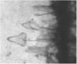
Some structures appear at the rear of the film, as shown in figure 2. Note that, in this case, the film is horizontal, as in figures 1(c) and 1(d), but inside the tube. This avoids the boundary effects at the end of the tube discussed in § 4.1, and allows for the visualisation of the film's rear side.

Figure 2. Side view of the film 0.5 ms after the shock. The vertical lines at the left of the figure are the trace of the meniscus and thus indicate the initial position of the film. In that case, the film is produced in the tube, and boundary effects are smaller. This allows us to visualise the structures which develop at the rear side of the film. The scale bar is 2 mm.
The behaviour shown in figures 1(c), 1(d) and 2 is not predicted by the theory developed in Bremond & Villermaux (Reference Bremond and Villermaux2005) and is studied on a controlled system in the following.
3. Experimental set-up
3.1. Materials and methods
The shock wave is produced with a shock tube, whose main characteristics are detailed hereafter. The low-pressure chamber is 1.2 m long and has a square section of  $30 \ \text {mm} \times 30\ \text {mm}$. Two opposite sides are made of polycarbonate, which is a transparent plastic. The high-pressure chamber is
  $200\ \text {mm}$ long. The shock is produced by perforating a
  $50\ \mathrm {\mu }\textrm {m}$ thick mylar sheet used as a diaphragm. We visualised the shock wave with a shadowgraph to check that no parasit reflection occurs in the tube. Even in the standard illumination conditions used for the experiments, the shock wave is visible in the images.
The pressure signal is recorded using four pressure sensors, PCB 113B28, located at  $85, 115, 145 \ {\rm and} \ 175\ \text {mm}$ from the end of the tube. The time resolution
  $\tau _{osc}= 1\ \mathrm {\mu } \text {s}$ is set by the oscilloscope sampling rate.
The foaming solution is made of a commercial dish-washing product (Dreft, Procter and Gamble) ( $10\,\%$ in volume) and glycerol (
 $10\,\%$ in volume) in water, of density
  $\rho _{w} = 10^3\ \textrm {kg}\ \textrm {m}^{-3}$. The liquid/air surface tension is
  $\sigma = 27\ \textrm {mN}\ \textrm {m}^{-1}$. The foam film is produced at the end of the tube by pulling a metallic frame of width 50 mm, height 100 mm and thickness 3 mm out of a bath (see figure 3). The inner boundary of the frame is bevelled and is only 1 mm thick. The equilibrium position of the film is in the rear plane of the frame (i.e. on the tube side), located 5 mm from the tube exit.

Figure 3. Experimental set-up. The shock tube is oriented along the axis  $x$ (horizontal). A frame is pulled out of the foaming solution reservoir at a controlled velocity to produce a foam film at the end of the tube, in the
  $(y,z)$ plane. The high-speed camera (HC) provides a side view of the film deformation and the spectral camera (SC) records the mirror reflection of a halogen light on the film, and thus measures the film thickness profile along the vertical direction
  $z$.
$z$.
This geometry is similar to the one used in Bremond & Villermaux (Reference Bremond and Villermaux2005). The originality of our study lies in the foam film thickness profile. Using successively a slow and a fast velocity to pull the frame out of the bath, we obtain a film with two well-defined thicknesses: the thinner part is in the top half of the frame and the thicker part in the bottom half, with a well-defined horizontal frontier separating both regions. The motor is stopped when the frame is centred on the tube axis. At this final position, the frame is fully out of the bath and we tuned the duration of the slower frame motion for the frontier to be in the middle of the film. We generate the shock wave 5 s after the motor stops, which results from a compromise between (i) a delay long enough for the film to stabilise and (ii) a delay short enough to minimise gravitational drainage in the film.
The chosen reference frame  $(0, \boldsymbol {e}_x, \boldsymbol {e}_y, \boldsymbol {e}_z)$ is shown in figure 3: the origin is in the film plane, in the middle of the frontier, the wave propagates in the
  $x$ direction and gravity is
  $-g \,\boldsymbol {e}_z$. The time at which the shock reaches the film is considered as the origin of times.
The thickness is measured as a function of  $z$ using a spectral camera, Resonon Pika L. The camera makes the image of a vertical line, ranging from the top to the bottom frame edge, in the central part of the film. This is a one-dimensional image, in the spatial direction of the camera sensor. The film is lit with a halogen lamp at an incidence angle
  $\alpha = 30^{\circ }$ and the spectrum reflected by each point of the imaged line is recorded in the spectral direction of the camera sensor. There are 900 pixels in the spatial direction, and 600 pixels in the spectral one, with a spectral resolution of approximately 1.06 nm. The wavelength of the light is in the range
  $[389 \text {--} 1025]\ \text {nm}$.
The intensity  $I$ reflected by a point
  $z$ of the imaged line is given, in the limit of large transmission coefficient, by
 \begin{equation} I(z,\lambda)=I_0 \left[1-\cos\left(\frac{4{\rm \pi} h(z) }{\lambda}\sqrt{n^2-\sin(\alpha)^2}\right)\right] , \end{equation}
with  $\lambda$ the wavelength,
  $I_0$ the incoming intensity,
  $\alpha$ the incidence angle,
  $n$ the refractive index of the solution and
  $h(z)$ the local thickness of the film.
The delay between two images is 4 ms, which is much larger than the dynamics of interest, but much shorter than the spontaneous evolution time of the film, before the shock. We thus only analyse the last image before the shock, which allows us to compute the thickness profile of the film  $h(z,t=0)$ at the time of the shock. We assume a thickness invariance in the
  $y$ direction, which is validated by visual inspection.
Finally, the film motion is recorded using a fast camera Photron fastcam sa-x2 type 1080k used at a rate between  $100\,000$ and
  $144\,000$ frames per second. The film is observed in transmission, using a Dedolight DLH400DT spot, powerful enough to use an exposure time of
  $0.3 \ \mathrm {\mu }\textrm {s}$. Most of the experiments have been performed with the direction of observation being along the
  $y$ direction (hereafter called the ‘side view’ position). Some additional observations have been made with a direction of observation making an angle of
  $15^{\circ }$ with the
  $x$ direction, in the
  $(x,y)$ plane (hereafter called the ‘front view’ position). In that case, the film is lit through the polycarbonate sides of the tube, which considerably degrades the image quality.
The fast camera and the pressure sensors are synchronised, and triggered by the arrival of the shock wave at the first pressure sensor. A dedicated reference image has been taken using the spectral camera and the fast camera to convert the spatial coordinates of both into the same reference frame.
3.2. Film thickness profiles
To produce the film, we first pull the frame, initially fully immersed, at a velocity  $V_1 \approx 0.6\ \textrm {mm}\ \textrm {s}^{-1}$. When approximately half the frame is out of the bath, the motor velocity switches abruptly to a much higher, tuneable, velocity
  $V_2$. It is well known that, when a film is pulled out of a bath, its thickness increases with the pulling velocity (Mysels, Shinoda & Frankel Reference Mysels, Shinoda and Frankel1959). The film occupying the lower part of the frame will therefore be thicker than that occupying the upper part. In all of the following, and despite the fact that all thickness values are of the same order of magnitude, we shall therefore talk about thin (upper part,
  $z>0$) and thick films (lower part,
  $z<0$).
A raw space-spectrum image of the resulting film, made just after the motor stops, is shown in figure 4, as well as the corresponding film thickness profile, deduced from (3.1). The thickness gradients in the transition domain are too large and the interference pattern is lost. The width of the unresolved zone is of the order of 1 mm, which is our error bar on the frontier position  $z=0$, located in the middle of this zone.

Figure 4. Characterisation of the film profiles. (a) Example of raw image of the spectral camera (last image before the shock). (b) Corresponding film thickness profile  $h(z)$ obtained using the relation (3.1). (c) Film thicknesses
  $h_1$ (diamonds) and
  $h_2$ (full circles) as a function of the motor velocity
  $V_2$.
The thin part of the film is very uniform and the thickness  $h_1$ is defined as
  $h_1= \langle h(z,t=0) \rangle _{z>0}$. The thickness of the lower part slightly varies with
  $z$, and we call
  $h_2$ the thickness measured at the first resolved point near the frontier, on the thick region side.
We attempted to tune the film thicknesses by varying  $V_2$, in the range
  $[10\text {--}200]\ \textrm {mm}\ \textrm {s}^{-1}$. However, as shown in figure 4, no significant thickness variation was obtained, and we have
  $h_1 = (1.12 \pm 0.1)$ and
  $h_2= (2.1 \pm 0.2)\ \mathrm {\mu }\textrm {m}$ for the whole set of data presented in this paper. The relevant dimensionless parameter in the problem is
  $(h_2-h_1)/h_1 \approx 1$. The fact that this ratio is of order unity in the problem justifies the denominations ‘thin’ and ‘thick’ films, which indicate the relative thickness and not the absolute one.
The thickness in the thick film increases in a band of width 5 mm along the frontier and then saturates. The order of magnitude of this gradient is  ${\mathrm {d}h}/{\mathrm {d}z}=-(0.13 \pm 0.05)\ \mathrm {\mu }\textrm {m}\ \textrm {mm}^{-1}$.
3.3. Wave properties
Typical pressure signals obtained with the empty tube are shown in figure 5 as a function of time. The high-pressure chamber of the tube is filled with air at the desired pressure. The diaphragm is then punched, ensuring the creation of the shock wave whose Mach number is perfectly determined. To investigate the influence of the Mach number on the system dynamics, experiments were performed with Mach numbers lying in the range [1.15–1.35]. The corresponding pressure jump across the shock wave, according to Rankine–Hugoniot relationships, then lies in the range [0.4–1] bar. The duration of the pressure plateau shown in figure 5 is limited by the reflection of the shock on the tube exit, leading to a rarefaction wave propagating backwards. The fast camera acquisition starts as the wave reaches the first pressure sensor, which synchronises both measures.

Figure 5. Pressure signals as a function of time for the empty tube, at sensors 1 (orange), 2 (green), 3 (blue) and 4 (dark blue); the different apparatus of the set-up are triggered by the sudden increase of the signal at sensor 1. Note that this graph is a raw experimental recording and has therefore a different time origin (wave arrival at sensor 1) than that we are using for our analysis in the following (wave impact on the film).
The shock Mach number is measured in the tube, at 10 cm from the end of the tube. The pressure front arrives, respectively, at times  $t_1$ and
  $t_4$ at sensors 1 and 4 separated by a distance
  $\ell = 90\ \text {mm}$. The Mach number is therefore
  ${M} = \ell /[a_0(t_4-t_1)]$, where
  $a_0 = \sqrt {\gamma rT_0} = \sqrt {{\gamma P_0}/{\rho _0}} =340\ \textrm {m}\ \textrm {s}^{-1}$ is the sound velocity in air, in the reference state. Here,
  $r$ and
  $\gamma = 1.4$ are the specific ideal gas constant and the adiabatic exponent;
  $T_0$,
  $P_0$ and
  $\rho _0$ are the temperature, pressure and density of the driven gas at rest.
When exiting the tube, the wave undergoes a progressive decay due to the large and abrupt area change, causing a diffraction phenomenon. According to Sloan & Nettleton (Reference Sloan and Nettleton1975), for a cylindrical shock tube of diameter  $D$, the shock decay on the symmetry axis will only become significant after a distance
  $L_{decay}$ measured from the tube exit, given by
 \begin{equation} L_{decay} = \dfrac{1}{2}D\cot\beta , \quad \text{with} \ \tan^2\beta = \frac{({M}^2 - 1)\left[(\gamma-1){M}^2 + 2\right] }{(\gamma+1){M}^4}. \end{equation}
 For the explored Mach number range in our study, and considering the hydraulic diameter of the tube,  $L_{decay}$ varies between 2.8 and 3.4 cm, which is much larger than the 5 mm distance separating the tube exit and the frame. Given those considerations, in a central part near the axis, the wave properties remain constant until it impacts the liquid film (figure 6). In the outer part, further from the axis, because of wave curvature and decay, the propagation of the wave and its interaction with the film are more complex. This will induce a delay in putting the film into motion in this area. The global shape of the film after impact will then be similar to that of the shock wave just before impact.

Figure 6. (a) Schematic side view (in the  $y$ or
  $z$ direction) of the propagation of the shock wave at the exit of the tube. The decay length
  $L_{decay}$ is given by (3.2). (b) Image of a transmitted shock wave, propagating to the right, in front of the film.
The impact of the shock wave on the film sets the latter into motion, leading to the creation of another shock wave downstream of the film. This wave will hereafter be referred to as the transmitted wave. The corresponding mechanism is described in § 5.1. The resulting wave can be tracked from the images (see figure 6b) and its Mach number  ${M}_{ext}$ can be retrieved. In figure 7, we plot the Mach number ratio
  ${{M}_{ext}}/{{M}}$ as a function of
  ${M}$, which appears to remain smaller than unity. The downstream wave is therefore always slower than the incident one, and this effect is more pronounced as
  ${M}$ increases. In all the following, data (averaged over approximately three experiments) are displayed for five different averaged Mach numbers, as shown in figure 7: 1.17, 1.22, 1.26, 1.29 and 1.32.

Figure 7. Transmitted to incident shock wave Mach number ratio as a function of the incident shock wave Mach number. For the sake of clarity, results were grouped and averaged over five different Mach number ranges, hence justifying the horizontal error bars. Vertical error bars stand for the experimental dispersion on the transmitted shock wave Mach number measurements.
4. Experimental results
4.1. Qualitative behaviour
Figure 8 shows the film dynamics after the shock has impacted the film. Because of the divergence of the flow at the exit of the tube, the lateral parts of the film (which is slightly larger than the tube exit) are accelerated by a smaller overpressure and reach a smaller velocity, therefore inducing a film curvature, as shown in figure 6(a). This effect accounts for the domain with fluctuating grey levels in figure 8, which grows as the film is put into motion. In figure 8(b), the well-defined frontier separating the uniform, light grey, background at large  $x$ and the darker part of the image, is thus the position
  $d(z,t)$ of the film in its planar, central part. In the following, we focus on that central part of the film and we assume that the problem does not depend on the
  $y$ coordinate.

Figure 8. (a) Definitions of  $d_1(z,t)$ and
  $d_2(t)$, the horizontal positions of, respectively, the thin and thick films (in the domain close to
  $y=0$, i.e. the central part of the film). The origin of the
  $x$ axis is located at the back of the solid frame, the latter corresponding to the uniform dark grey area; the origin of the
  $z$ axis is at the boundary between the thick and the thin parts of the film: the transparent orange strip coincides with the domain of unresolved thickness between both parts of the film, as measured with the spectral camera, and the point
  $z=0$ is set in the middle of the strip. The image used to define those quantities is the same as image (iv) on the right part of the figure. (b) Side views of the film after the shock impact. Image (i) is taken at
  $t=0$ (time of the impact on the film). The time interval between each frame is constant and is
  $20\ \mathrm {\mu }\textrm {s}$. The shock Mach number for this experiment was
  ${M}= 1.28$.
At impact, the suspended film is strongly accelerated and is torn from the frame and from its bounding menisci. Considering that the free boundary of the film retracts at the Taylor–Culick velocity (Taylor Reference Taylor1959; Culick Reference Culick1960; Keller Reference Keller1983),  $v_{TC}=[2 \sigma /(\rho _{w} h)]^{1/2} \approx 10\ \textrm {m}\ \textrm {s}^{-1}$ (in the film plane), the retraction after 0.5 ms is thus of the order of 5 mm. It is therefore reasonable to assume that the dynamics of the central part of the film remains unaffected by this process, in the observation time range.
As visible in figure 8(b) (and quantified in figure 11b), the whole film moves at a constant velocity after the shock. The thick part of the film, located at  $z<0$, remains relatively flat and parallel to its initial
  $(y,z)$ plane. On the contrary, the thin part shows a very different behaviour: it tilts and deforms, and the piece of film located close to the frontier moves slightly faster than the remaining part of the film.
After a delay of the order of  $100\ \mathrm {\mu }\textrm {s}$, the generation of a vortex is usually observed in the vicinity of the frontier, as shown in figure 9: the fastest point wraps around itself and holes appear in this strongly deformed region, as shown in figure 10, obtained with the camera in front view position. In the latter figure, the dark domain growing along the frontier position indicates a large tilt of the film with respect to its initial orientation. The first holes appear in this deformed region (figure 10d), and some rapidly expanding circular holes are clearly visible on the next images. The expansion velocity in this example is
  $7\ \textrm {m}\ \textrm {s}^{-1}$, consistent with the Taylor–Culick velocity of a
  $1\ \mathrm {\mu }\textrm {m}$ thick film.

Figure 9. Magnified view of the images displayed in figure 8, focusing on the growth of the perturbation at the interface between the thin and thick parts of the film.

Figure 10. Front views of the film after the shock impact. The first image is taken at time  $t=67\ \mathrm {\mu }\textrm {s}$. The time interval between each frame is
  $40\ \mathrm {\mu }\textrm {s}$. In (a), the darker line is located along the boundary between the thin and the thick parts of the film, initially at
  $z=0$ in (a). The width of this deformed strip increases with time. In (d), the first holes appear in the middle of the dark strip and expand in the following images, at the Taylor–Culick velocity. The black arrows in images (d,e) allow us to follow the growth of a particular hole.
4.2. Quantitative analysis of the film dynamics
4.2.1. Film's geometrical properties
In order to quantify the film dynamics before its rupture, we systematically extracted different geometrical quantities from the side view images, as shown in figure 11(a). The film shape, observed in its central part, is characterised by the equation  $x=d(z,t)$. As previously discussed, the foam film is expected to be initially in the rear plane of the frame, which we chose as reference for
  $x$ (see figure 8a). The first image where the shock is visible at the right of the frame is our experimental definition of the reference time
  $t=0$. With these conventions,
  $d(z,0)=0$ and
  $d(z,t)>0$ at later times.

Figure 11. (a) Definition of the geometrical quantities  $d_2$,
  $d_{1,max}$ and
  $A$. (b) Position
  $d_2$ of the thick part of the film as a function of time. The displayed lines correspond to the averaged Mach numbers defined in § 3.3: 1.17 (dark blue), 1.22 (blue), 1.26 (turquoise), 1.29 (green) and 1.32 (orange). The shaded area stands for the experimental dispersion on the turquoise curve (
 $M = 1.26$). The initial position of the film,
  $x_0$, obtained from the fitting procedure described in § 4.2.2, has been subtracted from
  $d_2$ for better readability.
We determined the frontier position  $z=0$ as the beginning of the film deformation, on the fastcam images. We checked that this point is consistent with the frontier position determined from the spectral camera data (see figure 8). As the thick film remains flat, its position
  $d_2(t)$ is obtained from an average over the whole
  $z<0$ domain. All the pixel lines between the image bottom and
  $z=0$ are first summed up. Along this averaged profile, the grey level shows a sharp decrease: the middle of this jump is automatically detected, providing the experimental definition of
  $d_2(t)$.
For the thin part of the film, we extracted  $d_{1,max}$, which is the position
  $d(z_{max})$ of the fastest point. Finally, we measured the whole area
  $A$ between the thin film profile
  $x= d_1(z,t)$ and the thick film position
  $x=d_2(t)$ for
  $0<z<z_{top}$ where
  $z_{top}$ is the upper limit of the image
 \begin{equation} A(t) = \int_0^{z_{top}} \left[d_1(z,t) - d_2(t)\right]\mathrm{d}z. \end{equation}
4.2.2. Film trajectory
The thick film trajectory, characterised by the time evolution of  $d_2$, is shown in figure 11. The acceleration time scale, of the order of a microsecond, is below our temporal resolution, and the dominant observed feature is thus a global motion of the whole film at a constant velocity
  $U$. Consistently, all the trajectories are well fitted by the law
  $d_2(t) = x_0 + U t$.
We defined the origin of the  $x$ axis as the rear side of the frame, which is the equilibrium position of the foam film. Consistently, the initial positions deduced from the fits verify
  $\langle x_0 \rangle = 0$, when averaged over all the data. However, the standard deviation
  $\delta x_0 = 2$ mm is large, and cannot be explained by the uncertainty on the impact time, which is the
  $10\ \mathrm {\mu }\textrm {s}$ delay between two images. This dispersion is probably due to some foam film vibrations induced by the fast pulling of the frame. The initial position has been subtracted on the trajectories shown in figure 11.
In figure 12, the obtained thick film velocities  $U$ are plotted as a function of the Mach numbers
  ${M}$ and
  ${M}_{ext}$ (defined in § 3.3). Whatever the chosen definition for the Mach number, we observe a global trend suggesting an increase of the film terminal velocity with the shock magnitude. The comparison with the film velocity
  $U_{{lin}}$ predicted in § 5 shows that the film velocity is compatible with an actual shock Mach number between
  ${M}$ and
  ${M}_{ext}$.

Figure 12. Velocity of the thick film  $U$ as a function of the Mach numbers
  ${M}$ (circles) and
  ${M}_{ext}$ (squares). This film velocity is compared to the prediction of (5.9) (solid line).
4.2.3. Local film deformation at the border between its thin and thick parts
The film deformation can be characterised by the difference  $d_{1,max}-d_2$, which is plotted as a function of time in figure 13. This quantity regularly increases after the shock impact, until it reaches typically one millimetre after a fraction of a millisecond. The fastest point therefore moves at a velocity of the order of
  $3\ \textrm {mm}\ \textrm {s}^{-1}$ relatively to the thick part, which is much smaller than the average film velocity
  $U$, of the order of
  $50\ \textrm {m}\ \textrm {s}^{-1}$: the thickness difference does not affect the global motion of the film. The one millimetre shift is in contrast very large compared to the film thickness, and corresponds to a dramatic deformation, leading to the film burst. The largest Mach numbers lead, on average, to slightly larger shifts, but the difference observed is smaller than the data dispersion.

Figure 13. Film position difference  $d_{1,max}- d_2$ as a function of time. The displayed lines correspond to the same averaged Mach numbers presented in figure 11. The shaded area stands for the experimental dispersion on the turquoise curve (
 $M = 1.26$).
A more global characterisation of the deformation is the area  $A$ defined in (4.1). This will be discussed in § 5.3.
5. Model
5.1. Shock impact on a uniform film
5.1.1. Assumptions of the model
The model discussed below to describe the shock impact on a film of uniform thickness has been proposed in Bremond & Villermaux (Reference Bremond and Villermaux2005). For the sake of clarity, the main features are recalled hereafter.
We consider an ideal, inviscid gas of specific heat ratio  $\gamma =1.4$, initially at rest at pressure
  $P_0$ and density
  $\rho _0$ (state 0). An incoming planar, steady, shock wave propagates in the gas at celerity
  $c$. Figure 14 shows a wave diagram of the phenomena at stake. The incident shock wave is characterised by its Mach number
  ${M} = c/a_0$. Behind the shock wave, the gas is brought to pressure
  $P_{a}$ and velocity
  $u_{a}$ (state (a) in figure 14), which can readily be determined using Rankine–Hugoniot relationships, which read
 \begin{gather} u_{a}= \frac{ 2 a_0}{\gamma+1}\left ({M} - \frac{1}{{M} }\right) , \end{gather}
 \begin{gather}P_{a}= P_0\frac{2}{\gamma+1} \left(\gamma {M}^2 - \frac{\gamma -1}{2} \right) . \end{gather}
Figure 14. Schematic of the different waves during the acceleration stage. The dotted lines indicate the characteristic lines used to relate the properties of the gas at a point on the film to its known properties in the state (0) (downstream) or in the state (a) (upstream). The position  $x^\ast$ and time
  $t^\ast$ at which the transmitted shock appears are also indicated. See text for further details.
At  $t=0$, the shock wave reaches the foam film, which is assumed to remain rigid and airtight. Since the film has a much higher acoustic impedance than the surrounding medium, the shock wave is fully reflected as a shock moving upstream. The gas properties behind the reflected shock wave are thus
  $u_{{b}} = 0$, and
  $P_{b}$ (state (b) in figure 14), given by (Courant & Friedrichs Reference Courant and Friedrichs1999)
 \begin{equation} \frac{P_{b}}{P_{a}}= \frac{(3 \gamma-1)\dfrac{P_{a}}{P_0} - (\gamma -1)}{(\gamma-1) \dfrac{P_{a}}{P_0} +(\gamma +1)} . \end{equation}
 The foam film, at position  $x_{f}$, is accelerated by the pressure difference
  $P(x_{f}^-,t)- P(x_{f}^+,t)$. Just after the shock impinges on the film,
  $P(x_{f}^-,0)= P_{b}$ and
  $P(x_{f}^+,0) = P_0$. However, at later times, the film motion produces a compressive wave downstream which increases the value of
  $P(x_{f}^+)$ and a relaxation wave upstream which decreases
  $P(x_{f}^-)$. After a characteristic time
  $\tau$ discussed below, the upstream and downstream pressures converge to the same value and the foam film reaches its asymptotic velocity
  $U$.
$U$.
To compute the foam film motion  $x_{f}(t)$, we need to determine the pressures
  $P(x_{f}^-,t)$ and
  $P(x_{f}^+,t)$ on both sides of the film. The film, essentially playing the role of a rigid piston, moves towards a gas of initial properties
  $P_0$,
  $u_0=0$, at a velocity
  ${\mathrm {d}x_{f}}/{\mathrm {d}t}$. The ensuing compressive wave turns into a shock wave after a time
  $t^\ast = ({2}/({\gamma +1}))({a_0}/{\varGamma _0})$ (Courant & Friedrichs Reference Courant and Friedrichs1999), where
  $\varGamma _0 = ({P_{b} - P_0})/{\mu }$ is the initial acceleration of the film, and
  $\mu$ the mass of the film per unit surface. The corresponding position is
  $x^\ast = a_0t^\ast$. For the pressure levels involved in our study,
  $t^\ast$ is of the order of a microsecond. Due to the non-isentropic nature of both reflected and transmitted shock waves, and their respective interactions with the expansion and compression waves, it is not possible to obtain an analytical expression for
  $P(x_{f}^-,t)$ and
  $P(x_{f}^+,t)$ for any given Mach number
  ${M}$. This can nevertheless be achieved for a weak incident shock wave (i.e.
  ${M} \approx 1 + \epsilon$).
5.1.2. Weak shock limit
Assuming all the involved shock waves are weak, the expansion and compression waves generated by the motion of the piston can be considered as simple waves. Indeed, Riemann invariants vary as  $({(P_{II}-P_{I})}/{P_{I}})^3$ across a shock connecting generic states (
 $I$) and (
 $II$), which leads to negligible variations across a weak shock wave (Courant & Friedrichs Reference Courant and Friedrichs1999). In that framework, states (b) and (c) shown in figure 14 are simple waves propagating respectively behind the reflected and transmitted shock waves. Consequently, taking into account the fact that, for an ideal gas,
  $a^2 = {\gamma P}/{\rho }$, the Riemann invariant conservation for the compression and expansion waves, read, respectively (Courant & Friedrichs Reference Courant and Friedrichs1999)
 \begin{gather} \frac{2}{\gamma-1} \sqrt{\frac{\gamma P(x_{f}^+) }{\rho(x_{f}^+)}} - \frac{\mathrm{d}x_{f}}{\mathrm{d}t} = \frac{2}{\gamma-1} \sqrt{\frac{\gamma P_0 }{\rho_0}} , \end{gather}
 \begin{gather}\frac{2}{\gamma-1} \sqrt{\frac{\gamma P(x_{f}^-) }{\rho(x_{f}^-)}} + \frac{\mathrm{d}x_{f}}{\mathrm{d}t} = \frac{2}{\gamma-1} \sqrt{\frac{\gamma P_{b} }{\rho_{2}}} . \end{gather}
Finally, the film motion obeys
 \begin{equation} \rho_{w} h \frac{\mathrm{d}^2x_{f}}{\mathrm{d}t^2} = P(x_{f}^-) - P(x_{f}^+) , \end{equation}
and (5.3)–(5.6) constitute a closed set of equations predicting the film motion and the main properties of the pressure fields.
In the limit of small overpressures, we get, at first order in  $P_{a}-P_0$,
  $P_{b} - P_0 =2 \ (P_{a}-P_0)$,
  $P(x_{f}^+) = P_0 (1+ ({\gamma }/{a_0}){\mathrm {d}x_{f}}/{\mathrm {d}t})$ and
  $P(x_{f}^-) = P_{b} (1- ({\gamma }/{a_0}){\mathrm {d}x_{f}}/{\mathrm {d}t})$. The equation of motion thus becomes
 \begin{equation} \frac{\mathrm{d}^2x_{f}}{\mathrm{d}t^2} + \frac{2 P_0 \gamma}{a_0 \rho_{w} h} \frac{\mathrm{d}x_{f}}{\mathrm{d}t}= 2 \frac{ P_{a}-P_0}{\rho_{w} h}, \end{equation}
and the film velocity is given by
 \begin{equation} \frac{\mathrm{d}x_{f}}{\mathrm{d}t} = a_0 \frac{ P_{a}-P_0}{\gamma P_0} \left (1-\textrm{e}^{-{t}/{\tau}} \right) , \end{equation}
with  $\tau = a_0 \rho _{w} h / (2 \gamma P_{a})$. For a thickness
  $h= 1.5 \ \mathrm {\mu }\textrm {m}$, the characteristic time is
  $\tau = 1.5\ \mathrm {\mu }\textrm {s}$, leading to an acceleration time of the order of
  $5\tau \approx 7.5\ \mathrm {\mu }\textrm {s}$. The asymptotic velocity,
 \begin{equation} U_{lin}=a_0 \frac{ P_{a}-P_0}{\gamma P_0} = \dfrac{2a_0}{\gamma+1}\left({M}^2 -1\right) , \end{equation}
is independent of the thickness.
In the linear limit, this asymptotic film velocity verifies  $U_{lin}= u_{a}$, with
  $u_{a}$ the gas velocity behind the initial shock (see (5.1) and (5.2), Courant & Friedrichs Reference Courant and Friedrichs1999). As it also equals the gas velocity behind the transmitted shock, the initial and transmitted shocks are characterised by the same gas velocity, and thus by the same Mach number.
In figure 12, we plot  $U$ as a function of the Mach number measured in the tube and at the tube exit. We show that the prediction of (5.9) is between both data series, which confirms that
  ${M}$ overestimates the Mach number for which the model would fit the experimental data, and that
  ${M}_{ext}$ underestimates it. The observed deviations between the one-dimensional model and our experimental results are consistent with the fact that multi-dimensional effects are most likely not negligible in the experiments. The validation of such a model requires a dedicated experimental set-up to ensure a purely one-dimensional gas dynamics. This topic will be covered in a forthcoming paper.
5.2. Shock impact on the two-thickness film
5.2.1. One-dimensional model
The film trajectory is easily obtained, in the weak shock limit, by integrating (5.8)
 \begin{equation} x_{f}= U_{lin} \left[t - \tau \left(1-\textrm{e}^{-{t}/{\tau}}\right) \right] . \end{equation}
 The asymptotic velocity is independent of the film thickness, but the acceleration time varies as  $h$, and is thus
  $\tau _1$ for the thin part and
  $\tau _2$ for the thick part, with
  $\tau _1< \tau _2$. Assuming that each part of the film evolves independently of the other, and therefore that the one-dimensional (1-D) model of § 5.1 remains valid, we predict from (5.10) that the distance between both film parts should be
 \begin{equation} {\rm \Delta} x= U_{lin} \left (\tau_2 - \tau_1 + \tau_1 \,\textrm{e}^{-{t}/{\tau_1}}- \tau_2 \, \textrm{e}^{-{t}/{\tau_2}} \right) . \end{equation}
 This theoretical shift can be considered as constant value after  $5\tau _2 \approx 10 \ \mathrm {\mu }\textrm {s}$. Its corresponding asymptotic value is
 \begin{equation} {\rm \Delta} x_\infty = \frac{ P_{a}-P_0}{2 \gamma P_0 } \frac{\rho_{w} }{ \rho_0} (h_2-h_1) , \end{equation}
which is of the order of  $100\ \mathrm {\mu }\textrm {m}$. The shift predicted by this 1-D approach is noticeably smaller than the experimental value
  $d_{1,max} - d_2$ (figure 13). As a consequence, it cannot be accounted for by the kinematic of each independent part of the film. In the following section we show that the dynamics of the film deformation is instead governed by the existence of transverse phenomena.
5.2.2. Transverse flows
During the acceleration time, transient pressure gradients appear in the  $z$ direction, inducing gas fluxes across the plane
  $z=0$. We determine the scaling and the order of magnitude of these fluxes below, in the weak shock limit. To do so, we consider a simplified motion of the film, described hereafter.
From the 1-D model of paragraph 5.1, we consider that, schematically, for  $t \in [0; \tau _1]$ the incident shock wave has been reflected on the film, which is assumed to remain motionless. At
  $t=\tau _1$, the thin film is instantaneously put into motion at velocity
  $U_{lin}$ (figure 15). Consequently, pressures behind and ahead of the thin part are the same and read
  $P_0+{\rm \Delta} P$. For
  $t \in [\tau _1;\tau _2]$, which is the case shown in figure 16, the thin part moves at velocity
  $U_{lin}$ and the incident shock has been rebuilt downstream in the
  $z>0$ domain, whereas the thick film can still be considered as motionless; for
  $t > \tau _2$, both parts of the film move at velocity
  $U_{lin}$ and the initial shock has been rebuilt downstream for all
  $z$. In a very crude approach, we will determine the transverse fluxes as perturbations to this reference situation.

Figure 15. Velocity of the film, rescaled by the linear asymptotic velocity  $U_{lin}$ (5.9), as a function of dimensionless time
  $t/\tau _1$. Blue and red solid lines represent the 1-D model predictions for thin and thick parts, respectively (5.8). The dashed steps represent the simplified motion we are considering in this section. Based on the measured film thicknesses, and the definition of
  $\tau$ in § 5.1.2, we have taken
  $\tau _2 = 2\tau _1$.

Figure 16. Schematic view of the pressure and velocity fields on both sides of the thin film ( $z>0$) and thick film (
 $z<0$), in the weak shock limit, at a time
  $t$ between
  $\tau _1$ and
  $\tau _2$. The red, solid lines represent the shock waves, moving at a velocity
  $c \approx a_0$; the black arrows represent the gas velocities (with black dots for gas at rest); the grey background is representative of the pressure level:
  $P_0$ in white,
  $P_0+ {\rm \Delta} P$ in light grey and
  $P_0+ 2 {\rm \Delta} P$ in dark grey. The velocity of the film being noticeably smaller than that of the shock waves, we neglect the motion of the thin part at the considered time. (a) Prediction of the 1-D model of § 5.1, leading to unphysical discontinuities along the line segments
  $L_{u}$ and
  $L_{d}$. (b) Compression and rarefaction waves (respectively red and blue dashed lines) propagating along the
  $z$-direction at a velocity
  $a_0$, inducing a vertical flux downwards (respectively upwards) downstream of (respectively upstream) the film.
As shown in figure 16(a), the above reference scenario involves a pressure discontinuity along two segments  $L_{u}$ and
  $L_{d}$, respectively upstream and downstream of the film, over a time interval
  $\delta \tau = \tau _2-\tau _1$. Assuming that the sound velocity variations can be neglected in the weak shock limit, the segment lengths scale as
  $a_0\delta \tau$ and the associated pressure jump as
  ${\rm \Delta} P = P_{a}- P_0$, the initial shock amplitude. The system cannot sustain such a pressure discontinuity along the
  $z=0$ line, and waves propagating in the
  $z$ direction are generated, as shown in figure 16(b). The transverse velocities shown in this figure are consistent with the appearance of a vortex at these times, and with its orientation.
Along the segment  $L_{u}$, the vertical gas velocity
  $w_1$ induces (i) a compressive wave invading at the sound velocity a gas at pressure
  $P_0+ {\rm \Delta} P$ in the
  $z>0$ domain; (ii) a rarefaction wave invading a gas at pressure
  $P_0+ 2 {\rm \Delta} P$ in the
  $z<0$ domain. Taking into account only the vertical component of the flow, Riemann invariant conservation yields
 \begin{gather} P(L_{u}) = (P_0+ {\rm \Delta} P) \left(1+ \gamma \frac{w_1}{a_0}\right) , \end{gather}
 \begin{gather}P(L_{u}) = (P_0+ 2 {\rm \Delta} P) \left(1- \gamma \frac{w_1}{a_0}\right) . \end{gather}
 The continuity of velocities and pressures along  $L_{u}$ finally leads to
 \begin{equation} w_1 = \frac{a_0}{2 \gamma} \frac{{\rm \Delta} P}{P_0} = \frac{1}{2} U_{lin} . \end{equation}
 As the compressive and rarefaction waves propagate at the sound velocity, the gas set into motion at time  $\tau _2$ at velocity
  $w_1$ is in a domain of height
  $a_0\delta \tau$ in the
  $z$ direction. The corresponding pressure field is shown schematically in figure 16.
The same process arises along the segment  $L_{d}$, with a resulting negative
  $z$-velocity
  $w_2 = -w_1$.
At later times, for  $t> \tau _2$, the whole system is set into motion at the velocity
  $U_{lin}$ in the
  $x$ direction, and the pressure field around the film has relaxed towards
  $P_{a}$. However, the gas having a vertical velocity at time
  $\tau _2$ keeps moving by inertia. In the weak shock limit, the resulting downstream flux across the line
  $z=0$ along
  $L_{d} \sim a_0 \delta \tau$ is of the form
  $Q= w_1 L_{d}$
 \begin{equation} Q = K \frac{a_0}{2 \gamma} \frac{{\rm \Delta} P}{P_0} a_0 \delta \tau , \end{equation}
with  $\delta \tau = a_0 \rho _{w} \delta h / (2 \gamma P_0)$. In this equation, we have added an unknown numerical factor
  $K$ which underlines that, given the strong simplifications made in the model, this prediction should be considered as a scaling law, providing the dominant functional dependencies and the order of magnitude.
Since the transverse velocities are bounded by  $w_1$, given by (5.15), the induced density variations remain small in our case. The model therefore predicts that the excess volume change in time (per unit length in the
  $y$ direction)
  ${\mathrm {d}A}/{\mathrm {d}t}$ can be approximated by the transverse flux
  $Q$, given by (5.16), independent of time. Using
  $\delta \tau$ as the relevant time unit for the problem we finally predict
 \begin{equation} \frac{A}{A_0} = K \frac{t}{\delta \tau} \quad \mbox{with} \ A_0 = \frac{1}{2 \gamma} \frac{{\rm \Delta} P}{P_0} (a_0 \delta \tau)^2 . \end{equation}
 As the transverse wave propagates at the velocity  $w_1$, the penetration depth of the film deformation should scale has
  $z_{def}(t) \!=\! w_1 t$ in the
  $z$ direction. Using
  $A \sim z_{def}(t) (d_{1,max} \!-\! d_2)$, we obtain
 \begin{equation} d_{1,max} - d_2 = K' a_0 \delta \tau , \end{equation}
with  $K'$ a second numerical prefactor. With our simple model, the amplitude of the film deformation in the
  $x$ direction is thus a constant. A transient is of course expected, before saturating at this maximal deformation. These predictions are compared to the experimental results in the next section.
5.3. Comparison with experimental data
For each series, we determine the time,  $t_{max}$, at which the theoretical value
  $z_{def}(t)$ reaches the upper limit of the field of view. After this time, some part of the deformation is predicted to be out of the field of view and thus not measurable anymore. We measure the excess area
  $A$ as explained in § 4.2.1 for the time range
  $[0 \ t_{max}]$ and we rescale the measured area by
  $A_0$ defined in (5.17);
  $A_0$ depends on
  $\delta P$, which is determined for each series from the averaged asymptotic film velocity (see figure 12), using (5.1). The characteristic time
  $\delta \tau = a_0 \rho _{w} \delta h / (2 \gamma P_0)$ is determined using
  $\delta h = 1 \ \mathrm {\mu }\textrm {m}$. Finally, we average the rescaled values
  $A/A_0$ over all series. The result is plotted in figure 17(a) as a function of the rescaled time. Given the error bar, the result is compatible with the predicted linear law and a fitting of the experimental data leads to
  $K=1.5$.

Figure 17. (a) Rescaled excess area  $A(t)/A_0$, averaged over all data, as a function of time for all the experiments. The grey shaded area represents the dispersion of the data. The red, solid line is the linear prediction of (5.17) with the prefactor
  $K = 1.5$. (b) Film position difference
  $d_{1,max}- d_2$ as a function of time, rescaled by
  $a_0 \delta \tau$ (same data as in figure 13). The displayed lines correspond to different Mach numbers (same convention as in figure 11). The shaded area stands for the experimental dispersion on the turquoise curve (
 $M = 1.26$). The grey dotted line is the prediction of (5.18) with the prefactor
  $K' =2$.
The distance between both films, already shown in figure 13, is rescaled according to (5.18) and compared to a plateau in figure 17(b). As the vortex strongly deforms the film close to the frontier, the agreement is less good, but the order of magnitude is here again well predicted. The lateral extension of the deformation in the  $z$ direction
  $z_{def}(t)= w_1 t$, i.e. should be of the order of 3 mm after 0.1 ms (with
  $U_{lin}= 60 \ \textrm {m}\ \textrm {s}^{-1}$ (see (5.15))). This quantity is more difficult to define experimentally and has therefore not been systematically quantified. However, its order of magnitude that can be observed at short times, in figure 8, for example, and is in agreement with the prediction.
Despite its simplicity, the model thus correctly predicts the growth of the excess area in time, and the qualitative shape of the film.
We believe that the patterns observed in figure 2 are due to the same phenomenon: some thick patches are left behind the film, with their boundaries wrapping around themselves downstream, thus forming the observed mushroom shapes. The typical thickness pattern in the film is shown in the inset of figure 1(c): the thickness varies in the range [300–800] nm, with disordered patterns involving many length scales. The amplitude of the induced film deformations can only be seen in the side views, but, as these images are only 2-D projections of the shape, most of these fluctuations are hidden by one another. However, the slowest and fastest pieces of film are visible. In some cases, a relatively regular shape without a hole is observed (most often at the rear side of the film), for which the volume evolution can be measured. We have only a few examples satisfying these requirements, but we can deduce orders of magnitude of transverse fluxes from them. As discussed below, they compare nicely to our model.
One example is shown in figure 18. The average position  $x_{f}$ of the film is extracted and provides the film velocity
  ${\mathrm {d}x_{f}}/{\mathrm {d}t}$ (see (5.8)). We measure at different times the width
  $2 R_1$ of an individual structure and the position
  $x_{min}$ of its slowest part. We define
  $R_2 = x_{f}-x_{min}$ and the gas volume trapped in the structure as
  $\varOmega (t) ={\rm \pi} (R_2-R_1) R_1^2 + 2 {\rm \pi}R_1^3 /3$, approximating the structure shape by a cylinder with a hemispherical end. The volume is plotted as a function of time in figure 19 and shows a linear evolution, only due to the increase of
  $R_2$. The value of
  $R_1$ is constant with time and is interpreted as the radius of the initial patch of higher thickness. Following the assumption of our model, we expect a flux
  $Q_{u}$ given by (5.16) to occur along the perimeter
  $2 {\rm \pi}R_1$ of this thick patch. The prediction is thus
 \begin{equation} \varOmega^{th} = K2 {\rm \pi}R_1 t \frac{\rho_{w}}{\rho_0} \frac{a_0}{4 \gamma} \frac{{\rm \Delta} P} {P_0} \delta h , \end{equation}
where  $K$ is the same numerical pre-factor as that introduced in (5.16). The pressure difference
  ${\rm \Delta} P$ is deduced from the asymptotic film velocity
  $U_{lin}$ using (5.9),
  $R_1$ is the structure radius, averaged on the successive images, and the thickness difference
  $\delta h$ is kept as an adjustable parameter, to fit the measured values
  $\varOmega (t)$.

Figure 18. Zoom on an individual structure in the deformed film, at times 15, 20, 25, 30 and  $60\ \mathrm {\mu }\textrm {s}$ after the shock (which propagates downwards). The red and green segments in figure (c) represent respectively the lengths
  $R_2$ and
  $2 R_1$ of the structure of interest; the horizontal white line is the position
  $x_f$ of the film as defined in the text. Panel (d) shows the last measurable image of the sequence, as a hole, underlined in blue, appears. The scale bar in (a) is 1 mm.

The characteristics obtained for six structures are summarised in table 1. Quantitative comparisons with experiments would require us to measure the thickness field, which is out of the reach of our temporal and spatial resolutions. However, the colour pattern of figure 1(c) indicates thickness fluctuations with an order of magnitude of a few hundred nanometres (which is the thickness variation from one green strip to a pink one). The predicted thickness difference is thus in the expected range.
Table 1. Examples of analysed structures at the rear of the films. The structure width  $R_1$ is measured on a few successive images and averaged over time; the incoming shock amplitude
  ${\rm \Delta} P$ is deduced from the film mean asymptotic velocity
  $U$; the thickness difference
  $\delta h$ is deduced from the structure volume variation rate, using the prediction (5.19), in which
  $K$ has been set to 1.5 (see figure 17).

6. Conclusion
When a foam film is impacted by a shock wave, a previously established model showed that the asymptotic velocity  $U$ reached by the film does not depend on the film thickness. In this paper, we have studied the dynamics of a two-thickness liquid film subjected to a moderate shock wave. We evidenced that a sharp frontier between the thin and the thick films is strongly deformed, leading to the development of a liquid protrusion downstream of the thin film. This induces a strong and localised film deformation along the frontier, which turns into a tear line separating both parts of the film. This process has been quantified on films with controlled thickness gradients. An analytical model involving transverse fluxes was developed to explain those features in the weak shock limit. A scaling law was derived for the transverse flux, which was found to be in good agreement with the experimental results. We believe that the process at stake is also responsible for the original rupture patterns observed on horizontal films, which spontaneously exhibit patches of different thicknesses. It may thus play an important role in the destabilisation of 3-D foams interacting with a shock wave, and potentially influence the droplet size distribution resulting from the foam collapse. The link between these processes and the wave mitigation remains to be identified.
Acknowledgements
The authors thank J.-C. Potier for the design of the shock tube. The PhD of Q.R. was supported by the French MoD (DGA). This project has received funding from the European Research Council (ERC) under the European Union's Horizon 2020 research and innovation programme (grant agreement no. 725094).
Declaration of interests
The authors report no conflict of interest.


