


1 Introduction
Since the classical work of Strouhal (Reference Strouhal1878), Prandtl (Reference Prandtl1905) and von Kármán (Reference von Kármán1911) it is well known that the separation of turbulent flows along smooth surfaces is a very complex physical phenomenon (Williamson Reference Williamson1996). Moreover, separation is also a very important effect because it determines the overall performance of many engineering devices. On aircraft for instance, the performance of wings, flaps and the empennage is typically limited by flow separation but also the intake, fan, compressor and turbine of jet engines suffer from separation phenomena. Flow separation is also disadvantageous for many internal flows such as pumps and water turbines or even pipelines. Thanks to the recent improvements in computer power, numerical simulations of unsteady flow separation phenomena are now technically possible up to moderate Reynolds numbers. However, the separation and the reattachment locations are not fixed in space and time due to the action of stochastic turbulent flow motions and flow instabilities. Therefore quantitative predictions are still associated with significant uncertainties (Fröhlich et al. Reference Fröhlich, Mellen, Rodi, Temmerman and Leschziner2005). These uncertainties depend on the simulation approach (Šarić et al. Reference Šarić, Jakirlić, Breuer, Jaffrézic, Deng, Chikhaoui, Fröhlich, von Terzi, Manhart and Peller2007) and turbulence or subgrid-scale models (Temmerman et al. Reference Temmerman, Leschziner, Mellen and Fröhlich2003). Consequently, reliable measurements with well-controlled boundary conditions are needed for the verification or disproof of the computational fluid dynamics (CFD) approach as well as to prove the model assumptions. Furthermore, the overall accuracy of the measurements is extremely important as the quality of numerical predictions is ultimately determined by the quality of the validation data. In other words, if the experimental results are biased due to systematic errors, the numerical results can be precise (low random error) if the right equations are solved correctly, but they are still uncertain. This is fully analogous to measurements which can be precise but uncertain, for instance if the calibration of the measurement technique is inaccurate. Therefore, the accuracy of the validation data is of major importance as it determines the prediction capabilities of CFD simulations.
For the validation of numerical results and the analysis of flow physics, precise measurements have to be performed. Hot wire (HW) or hot film measurements offer the advantages of very high sampling rates and accurate results (Bailey et al.
Reference Bailey, Kunkel, Hultmark, Vallikivi, Hill, Meyer, Tsay, Arnold and Smits2010). However, either the probe itself or the structure that supports it often disturb the flow field. This is why laser Doppler anemometry (LDA) was frequently used in the past to allow for precise non-intrusive point measurements. For common working distances of approximately 30 cm, a resolution of
 $5~{\rm\mu}\text{m}$
can be achieved in measurement volumes with a length of 1 mm (Shirai et al.
Reference Shirai, Pfister, Büttner, Czarske, Müller, Becker, Lienhart and Durst2006). However, the disadvantage of these methods is that they provide only point-wise data. Instantaneous flow features over the whole domain cannot be measured using LDA or HW. Therefore, optical multi-point measurement techniques were developed to allow for the measurement of thousands of velocity vectors instantaneously without disturbing the flow or fluid properties. Thanks to these developments, today it is possible to assess questions associated with coherent turbulent flow motions by applying spatial correlations, performing wavenumber spectral analysis and applying other multi-point analysis techniques to the instantaneous vector fields. Unfortunately, accurate measurements are difficult to perform for a number of reasons. One reason is associated with the uncertainty and resolution of the measurements. This holds true in particular for near-wall flow phenomena, which are difficult to resolve with optical methods because of strong flow gradients and the presence of model surfaces (Kähler, Scholz & Ortmanns Reference Kähler, Scholz and Ortmanns2006; Kähler, Scharnowski & Cierpka Reference Kähler, Scharnowski and Cierpka2012b
). However, due to the strong improvements in laser and camera technologies, and due to enhanced computer power which allows for the use of sophisticated image analysis techniques, enormous progress has been made over previous years to reduce the measurement uncertainty (Kähler et al.
Reference Kähler, Astarita, Vlachos, Sakakibara, Hain, Discetti, La Foy and Cierpka2016).
$5~{\rm\mu}\text{m}$
can be achieved in measurement volumes with a length of 1 mm (Shirai et al.
Reference Shirai, Pfister, Büttner, Czarske, Müller, Becker, Lienhart and Durst2006). However, the disadvantage of these methods is that they provide only point-wise data. Instantaneous flow features over the whole domain cannot be measured using LDA or HW. Therefore, optical multi-point measurement techniques were developed to allow for the measurement of thousands of velocity vectors instantaneously without disturbing the flow or fluid properties. Thanks to these developments, today it is possible to assess questions associated with coherent turbulent flow motions by applying spatial correlations, performing wavenumber spectral analysis and applying other multi-point analysis techniques to the instantaneous vector fields. Unfortunately, accurate measurements are difficult to perform for a number of reasons. One reason is associated with the uncertainty and resolution of the measurements. This holds true in particular for near-wall flow phenomena, which are difficult to resolve with optical methods because of strong flow gradients and the presence of model surfaces (Kähler, Scholz & Ortmanns Reference Kähler, Scholz and Ortmanns2006; Kähler, Scharnowski & Cierpka Reference Kähler, Scharnowski and Cierpka2012b
). However, due to the strong improvements in laser and camera technologies, and due to enhanced computer power which allows for the use of sophisticated image analysis techniques, enormous progress has been made over previous years to reduce the measurement uncertainty (Kähler et al.
Reference Kähler, Astarita, Vlachos, Sakakibara, Hain, Discetti, La Foy and Cierpka2016).
A second difficulty results from the need to compare statistical values because it is inherent to turbulence that each instantaneous turbulent flow field is unique at each time instant and never reproducible in all its details due to uncertainties in the initial and boundary conditions and flow instabilities. However, the determination of statistically stable values requires long simulation/measurement times to collect enough uncorrelated data for averaging the ensemble. This holds true, in particular, for separated flows because the low-frequency events must be sufficiently sampled to obtain statistically stable values of the flow quantities (as a rule of thumb, the motion with the lowest frequency should be sampled at least 100 times to obtain statistically stable values). For this reason, stable experimental conditions and full control of the initial and boundary conditions are very important because if the experimental and numerical results are not converged, the validation approach is biased and becomes questionable.
A well-established generic flow addressing the problem of turbulent flow separation on smooth geometries is the flow over periodic hills (ERCOFTAC test case 81). This flow has been extensively studied using various numerical methods and subgrid models (Günther & von Rohr Reference Günther and von Rohr2003; Šarić et al. Reference Šarić, Jakirlić, Breuer, Jaffrézic, Deng, Chikhaoui, Fröhlich, von Terzi, Manhart and Peller2007; Hickel, Kempe & Adams Reference Hickel, Kempe and Adams2008; Manhart, Peller & Brun Reference Manhart, Peller and Brun2008). Šarić et al. (Reference Šarić, Jakirlić, Breuer, Jaffrézic, Deng, Chikhaoui, Fröhlich, von Terzi, Manhart and Peller2007) have shown that the results depend strongly on the CFD approach applied for the numerical integration of the equations (unsteady Reynolds-averaged Navier–Stokes equations, detached eddy simulations (DES), large eddy simulations (LES), direct numerical simulations (DNS)) and Temmerman et al. (Reference Temmerman, Leschziner, Mellen and Fröhlich2003) examined the strong sensitivity of the LES results on the turbulence models. DNS simulations do not rely on turbulence models and should give reliable results. However, this holds true only if all spatial and temporal scales are properly resolved. If turbulent large-scale structures exist in reality, whose length exceed the periodicity of the hills, the assumption of periodic boundary conditions may become questionable because the effect of the large-scale structure on the flow statistics cannot be resolved. Simultaneously, it is important to resolve all turbulent scales up to the Kolmogorov length in the whole domain because a reduced resolution would not cover direct dissipation processes correctly. However, even with DNS, this effort is computationally too expensive so that DNS results also do not resolve all physical flow processes at each point in the flow domain (Breuer et al. Reference Breuer, Peller, Rapp and Manhart2009).
To validate the numerical results, a periodic hill experiment was designed by Manhart at TU Munich (Rapp & Manhart Reference Rapp and Manhart2011), based on the geometry of the experiment of Almeida, Durão & Heitor (Reference Almeida, Durão and Heitor1993). Figure 1(a) shows a sketch of the facility and a drawing of the characteristic flow features in the measurement domain (b).
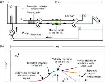
Figure 1. Overview of the periodic hill experiment at TU Munich adopted from Rapp & Manhart (Reference Rapp and Manhart2011) (a). Phenomenological map and coordinate system (b).
Existing particle image velocimetry and laser Doppler velocimetry measurements at
 $Re_{h}=5600$
to
$Re_{h}=5600$
to
 $Re_{h}=37\,000$
show the importance of the Reynolds stresses for the overall flow characteristics and the reattachment points (Rapp & Manhart Reference Rapp and Manhart2011). To cover the whole flow field in the streamwise plane with high resolution, the field of view had to be stitched together by an arrangement of six independent measurement series. As the measurements were not taken simultaneously within one experimental run, uncertainties in the boundary conditions cannot be avoided. Furthermore, a two-point correlation over the whole domain becomes impossible, thus hindering the possibility of evaluating the effect of coherent flow motions on the separation and reattachment locations, as well as the dynamics of the recirculation region. For this reason, the first objective of the current experiment was to use only one camera to cover the whole field of view in order to capture all flow phenomena at the same time within one experiment. The second aim was to apply modern evaluation techniques to reach a spatial resolution which is comparable with DNS and thus up to five times higher than the existing measurements. The acquisition of large data sets was the third objective of the present study to achieve converged values of the flow variables as requested by Fröhlich et al. (Reference Fröhlich, Mellen, Rodi, Temmerman and Leschziner2005).
$Re_{h}=37\,000$
show the importance of the Reynolds stresses for the overall flow characteristics and the reattachment points (Rapp & Manhart Reference Rapp and Manhart2011). To cover the whole flow field in the streamwise plane with high resolution, the field of view had to be stitched together by an arrangement of six independent measurement series. As the measurements were not taken simultaneously within one experimental run, uncertainties in the boundary conditions cannot be avoided. Furthermore, a two-point correlation over the whole domain becomes impossible, thus hindering the possibility of evaluating the effect of coherent flow motions on the separation and reattachment locations, as well as the dynamics of the recirculation region. For this reason, the first objective of the current experiment was to use only one camera to cover the whole field of view in order to capture all flow phenomena at the same time within one experiment. The second aim was to apply modern evaluation techniques to reach a spatial resolution which is comparable with DNS and thus up to five times higher than the existing measurements. The acquisition of large data sets was the third objective of the present study to achieve converged values of the flow variables as requested by Fröhlich et al. (Reference Fröhlich, Mellen, Rodi, Temmerman and Leschziner2005).
2 Experimental set-up and data evaluation
2.1 Water tunnel
The experiment was performed in a geostatic driven water tunnel at TU Munich. The channel is approximately 12 m in length with a total cross-section of
 $3.035h\times 18h$
(Rapp & Manhart Reference Rapp and Manhart2011). Ten hills with a height
$3.035h\times 18h$
(Rapp & Manhart Reference Rapp and Manhart2011). Ten hills with a height
 $h=50$
mm were mounted in a row to generate a mean periodic flow state around the seventh hill (see Rapp & Manhart (Reference Rapp and Manhart2011) and § 2.4). The distance between the hills in the streamwise direction was
$h=50$
mm were mounted in a row to generate a mean periodic flow state around the seventh hill (see Rapp & Manhart (Reference Rapp and Manhart2011) and § 2.4). The distance between the hills in the streamwise direction was
 $9h$
. The hills were made of blocks from polyurethane and thus feature a smooth surface with a roughness height lower than
$9h$
. The hills were made of blocks from polyurethane and thus feature a smooth surface with a roughness height lower than
 $1~{\rm\mu}\text{m}$
(Rapp & Manhart Reference Rapp and Manhart2011). In order to be able to measure the velocity field close to the wall, the flow was seeded with Rhodamin B doped polyamide particles with a diameter range of
$1~{\rm\mu}\text{m}$
(Rapp & Manhart Reference Rapp and Manhart2011). In order to be able to measure the velocity field close to the wall, the flow was seeded with Rhodamin B doped polyamide particles with a diameter range of
 $1{-}20~{\rm\mu}\text{m}$
. The particle Stokes number can be used to estimate the ability of the particles to follow the flow. The mean particle diameter was
$1{-}20~{\rm\mu}\text{m}$
. The particle Stokes number can be used to estimate the ability of the particles to follow the flow. The mean particle diameter was
 $10.3~{\rm\mu}\text{m}$
and the density
$10.3~{\rm\mu}\text{m}$
and the density
 ${\it\rho}_{P}=1.19~\text{g}~\text{cm}^{-3}$
. Following the analysis of Rapp & Manhart (Reference Rapp and Manhart2011) the particle time scale can be estimated to be
${\it\rho}_{P}=1.19~\text{g}~\text{cm}^{-3}$
. Following the analysis of Rapp & Manhart (Reference Rapp and Manhart2011) the particle time scale can be estimated to be
 $t_{d_{P\,max}}=2.65\times 10^{-5}$
s and
$t_{d_{P\,max}}=2.65\times 10^{-5}$
s and
 $t_{d_{P\,mean}}=7.03\times 10^{-6}$
s for the maximal and mean particle diameters, respectively. Using the maximum dissipation
$t_{d_{P\,mean}}=7.03\times 10^{-6}$
s for the maximal and mean particle diameters, respectively. Using the maximum dissipation
 ${\it\epsilon}_{max}$
from the DNS results of Peller et al. (Reference Peller, Le-Duc, Tremblay and Manhart2006) for
${\it\epsilon}_{max}$
from the DNS results of Peller et al. (Reference Peller, Le-Duc, Tremblay and Manhart2006) for
 $Re_{h}=5600$
and with proper scaling, the Kolmogorov time scale can be estimated to be
$Re_{h}=5600$
and with proper scaling, the Kolmogorov time scale can be estimated to be
 $t_{K,{\it\epsilon}_{max}}=0.24\times 10^{-3}$
s and
$t_{K,{\it\epsilon}_{max}}=0.24\times 10^{-3}$
s and
 $t_{K,{\it\epsilon}_{max}}=0.28\times 10^{-4}$
s for
$t_{K,{\it\epsilon}_{max}}=0.28\times 10^{-4}$
s for
 $Re_{h}=8000$
and
$Re_{h}=8000$
and
 $Re_{h}=33\,000$
, respectively. This gives a maximum Stokes number of
$Re_{h}=33\,000$
, respectively. This gives a maximum Stokes number of
 $St_{max}=t_{d_{P\,max}}/t_{K,{\it\epsilon}_{max}}$
of
$St_{max}=t_{d_{P\,max}}/t_{K,{\it\epsilon}_{max}}$
of
 $St=0.11$
for
$St=0.11$
for
 $Re_{h}=8000$
and
$Re_{h}=8000$
and
 $St_{max}=0.94$
for
$St_{max}=0.94$
for
 $Re_{h}=33\,000$
. Using the mean diameter and the mean dissipation
$Re_{h}=33\,000$
. Using the mean diameter and the mean dissipation
 $St_{mean}=0.61\times 10^{-2}$
for
$St_{mean}=0.61\times 10^{-2}$
for
 $Re_{h}=8000$
and
$Re_{h}=8000$
and
 $St_{mean}=0.05$
for
$St_{mean}=0.05$
for
 $Re_{h}=33\,000$
. Therefore, it can be assumed that the particles follow the flow faithfully on average. By equipping the camera with a low pass light filter, the reflections of the wall were almost completely suppressed. To avoid errors due to misalignment of the light sheet from two independent laser cavities, the light sheet in the mid-span of the channel was generated by a single cavity INOLASS laser in double pulse mode. For the image recording a sCMOS camera (PCO GmbH) was operated at 5 Hz for a total measurement time of approximately 1.2 h for each Reynolds number. In comparison to the measurements performed by Rapp & Manhart (Reference Rapp and Manhart2011), where the whole field of view had to be stitched together by a six separated camera arrangement, only one camera covering the whole field of view was used for the current investigation within a region of
$Re_{h}=33\,000$
. Therefore, it can be assumed that the particles follow the flow faithfully on average. By equipping the camera with a low pass light filter, the reflections of the wall were almost completely suppressed. To avoid errors due to misalignment of the light sheet from two independent laser cavities, the light sheet in the mid-span of the channel was generated by a single cavity INOLASS laser in double pulse mode. For the image recording a sCMOS camera (PCO GmbH) was operated at 5 Hz for a total measurement time of approximately 1.2 h for each Reynolds number. In comparison to the measurements performed by Rapp & Manhart (Reference Rapp and Manhart2011), where the whole field of view had to be stitched together by a six separated camera arrangement, only one camera covering the whole field of view was used for the current investigation within a region of
 $9h\times 3.035h$
. This provides a data set which also allows for statistically relevant two-point correlations of the whole flow field.
$9h\times 3.035h$
. This provides a data set which also allows for statistically relevant two-point correlations of the whole flow field.
As opposed to previous investigations, where the interaction of structures between consecutive hills and in the separation region was the focus (Rapp & Manhart Reference Rapp and Manhart2011; Schröder et al.
Reference Schröder, Schanz, Michaelis, Cierpka, Scharnowski and Kähler2015), the field of view was centred at the hill top to analyse the large-scale structures. The coordinate system is defined to have its origin in the
 $x$
-direction at the centre of the seventh hill and the bottom wall in the
$x$
-direction at the centre of the seventh hill and the bottom wall in the
 $y$
-direction (see figure 1
b). To achieve the best possible spatial resolution for each desired variable, the particle image distributions were evaluated with different approaches including standard correlation-based analysis for instantaneous vector fields (Scarano Reference Scarano2002). Ensemble-correlation methods are used for the mean velocity fields and mean Reynolds stresses (Scharnowski, Hain & Kähler Reference Scharnowski, Hain and Kähler2012). They give very reliable and accurate results with much higher spatial resolution compared to the use of standard particle image velocimetry (PIV) for the instantaneous fields (Kähler, Scharnowski & Cierpka Reference Kähler, Scharnowski and Cierpka2012a
; Kähler et al.
Reference Kähler, Scharnowski and Cierpka2012b
). Since standard PIV is known to act as a spatial low pass filter, due to the finite size of the interrogations windows, the method fails close to the wall where large velocity gradients are present. For this reason, particle tracking methods were applied to estimate the probability density functions of the velocity (Cierpka, Lütke & Kähler Reference Cierpka, Lütke and Kähler2013a
) close to the hill top.
$y$
-direction (see figure 1
b). To achieve the best possible spatial resolution for each desired variable, the particle image distributions were evaluated with different approaches including standard correlation-based analysis for instantaneous vector fields (Scarano Reference Scarano2002). Ensemble-correlation methods are used for the mean velocity fields and mean Reynolds stresses (Scharnowski, Hain & Kähler Reference Scharnowski, Hain and Kähler2012). They give very reliable and accurate results with much higher spatial resolution compared to the use of standard particle image velocimetry (PIV) for the instantaneous fields (Kähler, Scharnowski & Cierpka Reference Kähler, Scharnowski and Cierpka2012a
; Kähler et al.
Reference Kähler, Scharnowski and Cierpka2012b
). Since standard PIV is known to act as a spatial low pass filter, due to the finite size of the interrogations windows, the method fails close to the wall where large velocity gradients are present. For this reason, particle tracking methods were applied to estimate the probability density functions of the velocity (Cierpka, Lütke & Kähler Reference Cierpka, Lütke and Kähler2013a
) close to the hill top.
The temperature of the water was determined to be
 $19.7\,^{\circ }\text{C}$
and exhibited a change of approximately
$19.7\,^{\circ }\text{C}$
and exhibited a change of approximately
 $2\,^{\circ }\text{C}$
over the course of the measurement. The Reynolds number, based on the averaged velocity above the hill crest in the middle of the channel,
$2\,^{\circ }\text{C}$
over the course of the measurement. The Reynolds number, based on the averaged velocity above the hill crest in the middle of the channel,
 $u_{b}$
, and the hill height, was estimated to
$u_{b}$
, and the hill height, was estimated to
 $Re_{h}=u_{b}h/{\it\nu}=8000\pm 160$
and
$Re_{h}=u_{b}h/{\it\nu}=8000\pm 160$
and
 $Re_{h}=32\,600\pm 660$
, which will be referred to as 8000 and 33 000 respectively in the following.
$Re_{h}=32\,600\pm 660$
, which will be referred to as 8000 and 33 000 respectively in the following.
2.2 Convergence
In order to make a statistical analysis and comparison with numerical results it is important to ensure that the experimental mean values are converged, even for highly turbulent flows. For reference, the time required by an event or structure to travel with the mean convection velocity over the hill crest
 $u_{b}$
through one periodic part of the channel, i.e.
$u_{b}$
through one periodic part of the channel, i.e.
 $9h$
, was chosen. This reference time is denoted the ‘flow through time’ (Rapp & Manhart Reference Rapp and Manhart2011). For
$9h$
, was chosen. This reference time is denoted the ‘flow through time’ (Rapp & Manhart Reference Rapp and Manhart2011). For
 $Re_{h}=8000$
the reference time is
$Re_{h}=8000$
the reference time is
 $t_{ref}=9h/u_{b}=2.63$
s and
$t_{ref}=9h/u_{b}=2.63$
s and
 $t_{ref}=0.64$
s for
$t_{ref}=0.64$
s for
 $Re=33\,000$
. Since the acquisition rate of the double frame images was set to 5 Hz, a structure travelling with the mean flow is sampled within the field of view on 13 instantaneous flow fields for
$Re=33\,000$
. Since the acquisition rate of the double frame images was set to 5 Hz, a structure travelling with the mean flow is sampled within the field of view on 13 instantaneous flow fields for
 $Re=8000$
and 3 instantaneous flow fields for
$Re=8000$
and 3 instantaneous flow fields for
 $Re=33\,000$
, respectively. However, the low-frequency events are critical, especially for convergence. The measurement time was
$Re=33\,000$
, respectively. However, the low-frequency events are critical, especially for convergence. The measurement time was
 $1680\times t_{ref}$
in the case of
$1680\times t_{ref}$
in the case of
 $Re=8000$
and
$Re=8000$
and
 $6840\times t_{ref}$
for
$6840\times t_{ref}$
for
 $Re=33\,000$
, corresponding to
$Re=33\,000$
, corresponding to
 $22\,000$
or
$22\,000$
or
 $24\,000$
PIV image pairs, respectively. The number of flow through times was increased by at least a factor of 3 compared to previous experiments.
$24\,000$
PIV image pairs, respectively. The number of flow through times was increased by at least a factor of 3 compared to previous experiments.
Figure 2 shows the mean streamwise velocity and higher-order moments of the velocity fluctuations as a function of the measurement time. The velocity fields were computed by using a window-correlation-based PIV evaluation (including iterative window shifting, image deformation and adaptive window weighting) with a final interrogation window size of
 $16\times 16$
px and 50 % overlap, corresponding to a spatial resolution of 3 mm (
$16\times 16$
px and 50 % overlap, corresponding to a spatial resolution of 3 mm (
 ${\approx}0.06h$
). The three curves in each graph correspond to different locations within the flow field. The streamwise position was fixed to
${\approx}0.06h$
). The three curves in each graph correspond to different locations within the flow field. The streamwise position was fixed to
 $x/h=2$
for all points and the wall-normal positions are
$x/h=2$
for all points and the wall-normal positions are
 $y/h=0.5$
,
$y/h=0.5$
,
 $1.0$
and
$1.0$
and
 $2.0$
to study the convergence in the recirculation region, the shear layer and in the free stream region, respectively.
$2.0$
to study the convergence in the recirculation region, the shear layer and in the free stream region, respectively.
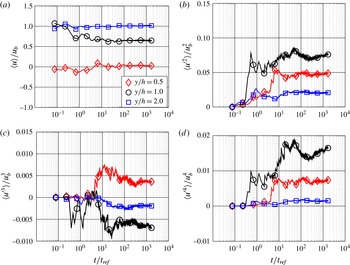
Figure 2. Evolution of the mean value for the streamwise velocity
 $u/u_{b}$
(a) and (b–d) the other streamwise higher-order moments for
$u/u_{b}$
(a) and (b–d) the other streamwise higher-order moments for
 $Re_{h}=8000$
at
$Re_{h}=8000$
at
 $x/h=2$
for three different wall-normal positions (
$x/h=2$
for three different wall-normal positions (
 $y/h=0.5;1.0;2.0$
).
$y/h=0.5;1.0;2.0$
).
The mean velocity converges for all points after approximately
 $200\times t_{ref}$
for
$200\times t_{ref}$
for
 $Re_{h}=8000$
and after approximately
$Re_{h}=8000$
and after approximately
 $800\times t_{ref}$
for
$800\times t_{ref}$
for
 $Re_{h}=33\,000$
(not shown). As expected, the mean velocity converges faster than the moments of the velocity fluctuations. Furthermore, the point in the free stream at
$Re_{h}=33\,000$
(not shown). As expected, the mean velocity converges faster than the moments of the velocity fluctuations. Furthermore, the point in the free stream at
 $y/h=2$
converges more rapidly than the one in the recirculation region at
$y/h=2$
converges more rapidly than the one in the recirculation region at
 $y/h=0.5$
, which on the other hand converges quicker than the point in the shear layer at
$y/h=0.5$
, which on the other hand converges quicker than the point in the shear layer at
 $y/h=1.0$
. It can be concluded from the results that the present data sets are well suited for the determination of statistically stable mean velocity values. For the estimation of the moments of the velocity fluctuations, the measurement time is sufficiently long for regions with low turbulence levels. The values in the shear layer as well as in the recirculation region might not be fully converged. However, increasing the measurement time further requires careful control of all parameters that might influence the flow, such as the temperature. It should be mentioned that the convergence time is 12 to 48 times longer than the time for ensemble averaging in the LES and DNS by Breuer et al. (Reference Breuer, Peller, Rapp and Manhart2009), where only 140 flow through times were resolved for
$y/h=1.0$
. It can be concluded from the results that the present data sets are well suited for the determination of statistically stable mean velocity values. For the estimation of the moments of the velocity fluctuations, the measurement time is sufficiently long for regions with low turbulence levels. The values in the shear layer as well as in the recirculation region might not be fully converged. However, increasing the measurement time further requires careful control of all parameters that might influence the flow, such as the temperature. It should be mentioned that the convergence time is 12 to 48 times longer than the time for ensemble averaging in the LES and DNS by Breuer et al. (Reference Breuer, Peller, Rapp and Manhart2009), where only 140 flow through times were resolved for
 $Re_{h}=700\ldots 10\,600$
. Fröhlich et al. (Reference Fröhlich, Mellen, Rodi, Temmerman and Leschziner2005) used 55 flow through times for their LES data for
$Re_{h}=700\ldots 10\,600$
. Fröhlich et al. (Reference Fröhlich, Mellen, Rodi, Temmerman and Leschziner2005) used 55 flow through times for their LES data for
 $Re_{h}=10\,600$
and Diosady & Murman (Reference Diosady and Murman2014) simulated the flow for 25 flow through times using DNS for the same Reynolds number. However, Diosady & Murman (Reference Diosady and Murman2014) state explicitly that this is not sufficient for statistical convergence, which was not the aim of their investigation.
$Re_{h}=10\,600$
and Diosady & Murman (Reference Diosady and Murman2014) simulated the flow for 25 flow through times using DNS for the same Reynolds number. However, Diosady & Murman (Reference Diosady and Murman2014) state explicitly that this is not sufficient for statistical convergence, which was not the aim of their investigation.
Spanwise averaging is often performed to increase the convergence in the case of numerical simulations to overcome the limitations due to the short sampling time (Fröhlich et al.
Reference Fröhlich, Mellen, Rodi, Temmerman and Leschziner2005; Breuer et al.
Reference Breuer, Peller, Rapp and Manhart2009). However, the correlated motion in the spanwise direction has a half-width of
 $z/h=3.5{-}4$
, as shown numerically by Mellen, Fröhlich & Rodi (Reference Mellen, Fröhlich and Rodi2000), Fröhlich et al. (Reference Fröhlich, Mellen, Rodi, Temmerman and Leschziner2005) and experimentally by Rapp & Manhart (Reference Rapp and Manhart2011). Mellen et al. (Reference Mellen, Fröhlich and Rodi2000) performed a numerical simulation for
$z/h=3.5{-}4$
, as shown numerically by Mellen, Fröhlich & Rodi (Reference Mellen, Fröhlich and Rodi2000), Fröhlich et al. (Reference Fröhlich, Mellen, Rodi, Temmerman and Leschziner2005) and experimentally by Rapp & Manhart (Reference Rapp and Manhart2011). Mellen et al. (Reference Mellen, Fröhlich and Rodi2000) performed a numerical simulation for
 $Re_{h}=7100$
using two different spanwise domain sizes
$Re_{h}=7100$
using two different spanwise domain sizes
 $z/h=4.5$
and
$z/h=4.5$
and
 $z/h=9.0$
. The separation region changed from
$z/h=9.0$
. The separation region changed from
 $x_{s}/h=0.5$
to
$x_{s}/h=0.5$
to
 $x_{s}/h=0.45$
and the reattachment point from
$x_{s}/h=0.45$
and the reattachment point from
 $x_{r}/h=3.2$
to
$x_{r}/h=3.2$
to
 $x_{r}/h=3.25$
. The difference in the mean flow field was moderate. However, the Reynolds stresses differ considerably. Due to computational limitations at the time of the study, the grid was relatively coarse. Finally, it was concluded that the subgrid model and the finer mesh influence the results to a larger extent, and therefore a spanwise domain of only
$x_{r}/h=3.25$
. The difference in the mean flow field was moderate. However, the Reynolds stresses differ considerably. Due to computational limitations at the time of the study, the grid was relatively coarse. Finally, it was concluded that the subgrid model and the finer mesh influence the results to a larger extent, and therefore a spanwise domain of only
 $z/h=4.5$
was used in later studies (Temmerman et al.
Reference Temmerman, Leschziner, Mellen and Fröhlich2003; Fröhlich et al.
Reference Fröhlich, Mellen, Rodi, Temmerman and Leschziner2005; Šarić et al.
Reference Šarić, Jakirlić, Breuer, Jaffrézic, Deng, Chikhaoui, Fröhlich, von Terzi, Manhart and Peller2007; Hickel et al.
Reference Hickel, Kempe and Adams2008; Manhart et al.
Reference Manhart, Peller and Brun2008; Breuer et al.
Reference Breuer, Peller, Rapp and Manhart2009; Diosady & Murman Reference Diosady and Murman2014; Chang et al.
Reference Chang, Jakirlić, Krumbein and Tropea2015). However, as the size of the computational domain in the spanwise direction is smaller than two times the size of a packet of structures, the convergence of the average solution using spanwise averaging might be accelerated, but it is questionable if this approach leads to the physically true values considering that the flow is correlated in the spanwise direction. Furthermore, it cannot be expected that a number of flow through times of the order of tens is sufficient to realize all possible turbulent flow events and to sample them frequently enough to obtain the true statistical values with sufficient confidence. The results in figure 2 suggest that at least 1000 flow through times are required to obtain the first- and second-order statistics correctly. However, the slow convergence of the third- and forth-order statistics illustrates that more samples are required to cover the effect of the extreme flow events, which are very rare.
$z/h=4.5$
was used in later studies (Temmerman et al.
Reference Temmerman, Leschziner, Mellen and Fröhlich2003; Fröhlich et al.
Reference Fröhlich, Mellen, Rodi, Temmerman and Leschziner2005; Šarić et al.
Reference Šarić, Jakirlić, Breuer, Jaffrézic, Deng, Chikhaoui, Fröhlich, von Terzi, Manhart and Peller2007; Hickel et al.
Reference Hickel, Kempe and Adams2008; Manhart et al.
Reference Manhart, Peller and Brun2008; Breuer et al.
Reference Breuer, Peller, Rapp and Manhart2009; Diosady & Murman Reference Diosady and Murman2014; Chang et al.
Reference Chang, Jakirlić, Krumbein and Tropea2015). However, as the size of the computational domain in the spanwise direction is smaller than two times the size of a packet of structures, the convergence of the average solution using spanwise averaging might be accelerated, but it is questionable if this approach leads to the physically true values considering that the flow is correlated in the spanwise direction. Furthermore, it cannot be expected that a number of flow through times of the order of tens is sufficient to realize all possible turbulent flow events and to sample them frequently enough to obtain the true statistical values with sufficient confidence. The results in figure 2 suggest that at least 1000 flow through times are required to obtain the first- and second-order statistics correctly. However, the slow convergence of the third- and forth-order statistics illustrates that more samples are required to cover the effect of the extreme flow events, which are very rare.
2.3 Spatial resolution
For the spatial resolution analysis, the Kolmogorov length scale
 ${\it\eta}$
of the experiment can be estimated by scaling the value of Breuer et al. (Reference Breuer, Peller, Rapp and Manhart2009) obtained for DNS data at
${\it\eta}$
of the experiment can be estimated by scaling the value of Breuer et al. (Reference Breuer, Peller, Rapp and Manhart2009) obtained for DNS data at
 $Re_{h}=5600$
with
$Re_{h}=5600$
with
 $Re^{-3/4}$
(Breuer et al.
Reference Breuer, Peller, Rapp and Manhart2009). This results in a mean Kolmogorov length scale of
$Re^{-3/4}$
(Breuer et al.
Reference Breuer, Peller, Rapp and Manhart2009). This results in a mean Kolmogorov length scale of
 ${\it\eta}\approx 100~{\rm\mu}\text{m}$
for
${\it\eta}\approx 100~{\rm\mu}\text{m}$
for
 $Re_{h}=8000$
and
$Re_{h}=8000$
and
 ${\it\eta}\approx 35~{\rm\mu}\text{m}$
for
${\it\eta}\approx 35~{\rm\mu}\text{m}$
for
 $Re_{h}=33\,000$
. Typical grid sizes for numerical simulations are of the order of several (3–10) Kolmogorov length scales
$Re_{h}=33\,000$
. Typical grid sizes for numerical simulations are of the order of several (3–10) Kolmogorov length scales
 ${\it\eta}$
at the wall for LES (Fröhlich et al.
Reference Fröhlich, Mellen, Rodi, Temmerman and Leschziner2005) and approach
${\it\eta}$
at the wall for LES (Fröhlich et al.
Reference Fröhlich, Mellen, Rodi, Temmerman and Leschziner2005) and approach
 ${\it\eta}$
for DNS (Breuer et al.
Reference Breuer, Peller, Rapp and Manhart2009). This comparison indicates that the resolution of the existing experimental data by Rapp & Manhart (Reference Rapp and Manhart2011) do not match the resolution of the simulations. In effect, the strong gradients in the boundary and shear layer could not be resolved. Even more severe is the fact that the contribution of the small eddies is averaged out due to spatial filtering. Thus, parts of the turbulent energy could not be measured. Since in LES the subgrid models are supposed to simulate the contribution of these small eddies, it is of inherent interest to increase the resolution in the experiment to cover the contribution of all scales.
${\it\eta}$
for DNS (Breuer et al.
Reference Breuer, Peller, Rapp and Manhart2009). This comparison indicates that the resolution of the existing experimental data by Rapp & Manhart (Reference Rapp and Manhart2011) do not match the resolution of the simulations. In effect, the strong gradients in the boundary and shear layer could not be resolved. Even more severe is the fact that the contribution of the small eddies is averaged out due to spatial filtering. Thus, parts of the turbulent energy could not be measured. Since in LES the subgrid models are supposed to simulate the contribution of these small eddies, it is of inherent interest to increase the resolution in the experiment to cover the contribution of all scales.
To illustrate the effect of the spatial filtering on the mean velocity profile close to the model surface, the measured data were evaluated with different resolutions. Interrogation windows of
 $32\times 32$
pixels provide a resolution of 6 mm,
$32\times 32$
pixels provide a resolution of 6 mm,
 $16\times 16$
pixels of 3 mm and
$16\times 16$
pixels of 3 mm and
 $8\times 8$
pixels of 1.5 mm. To further increase the spatial resolution for the mean values, the single-pixel ensemble correlation is an appropriate method (Scharnowski et al.
Reference Scharnowski, Hain and Kähler2012). This approach provides a velocity vector at each pixel location. However, the final resolution, i.e. the distance of independent velocity vectors, depends on the particle image size and not on the pixel size of the recording camera (Kähler et al.
Reference Kähler, Scharnowski and Cierpka2012a
). In the present experiment, the mean particle image diameter was estimated to be 2.4 pixels, which results in a resolution of 0.45 mm. The velocity field is therefore at least 5 times better resolved than in previous measurements (Rapp & Manhart Reference Rapp and Manhart2011). For
$8\times 8$
pixels of 1.5 mm. To further increase the spatial resolution for the mean values, the single-pixel ensemble correlation is an appropriate method (Scharnowski et al.
Reference Scharnowski, Hain and Kähler2012). This approach provides a velocity vector at each pixel location. However, the final resolution, i.e. the distance of independent velocity vectors, depends on the particle image size and not on the pixel size of the recording camera (Kähler et al.
Reference Kähler, Scharnowski and Cierpka2012a
). In the present experiment, the mean particle image diameter was estimated to be 2.4 pixels, which results in a resolution of 0.45 mm. The velocity field is therefore at least 5 times better resolved than in previous measurements (Rapp & Manhart Reference Rapp and Manhart2011). For
 $Re_{h}=8000$
and
$Re_{h}=8000$
and
 $Re_{h}=33\,000$
, a spatial resolution of
$Re_{h}=33\,000$
, a spatial resolution of
 $4.4{\it\eta}$
and
$4.4{\it\eta}$
and
 $12.7{\it\eta}$
was reached, respectively. These values are comparable to DNS (Breuer et al.
Reference Breuer, Peller, Rapp and Manhart2009) and of the order of the eddy length scales for 90 % of energy dissipation in isotropic turbulence, which is
$12.7{\it\eta}$
was reached, respectively. These values are comparable to DNS (Breuer et al.
Reference Breuer, Peller, Rapp and Manhart2009) and of the order of the eddy length scales for 90 % of energy dissipation in isotropic turbulence, which is
 ${>}8{\it\eta}$
(Pope Reference Pope2000).
${>}8{\it\eta}$
(Pope Reference Pope2000).

Figure 3. Mean velocity in
 $x$
-direction for
$x$
-direction for
 $Re_{h}=8000$
using
$Re_{h}=8000$
using
 $16\times 16$
pixel window correlation (a) and ensemble correlation (b).
$16\times 16$
pixel window correlation (a) and ensemble correlation (b).
A direct comparison of the mean flow fields using an interrogation window size of
 $16\times 16$
pixels and single-pixel ensemble correlation is shown in figure 3. Qualitatively, the results look quite similar and in fact they are almost identical. However, in the near-wall region, strong quantitative differences are present. This is illustrated in figure 4 where the velocity profiles close to the wall are shown for
$16\times 16$
pixels and single-pixel ensemble correlation is shown in figure 3. Qualitatively, the results look quite similar and in fact they are almost identical. However, in the near-wall region, strong quantitative differences are present. This is illustrated in figure 4 where the velocity profiles close to the wall are shown for
 $x/h=0.27$
(indicated with the green line and A in figure 3). The single-pixel ensemble-correlation results clearly indicate that the flow starts to separate whereas all window correlation results still reveal a rather large velocity in the
$x/h=0.27$
(indicated with the green line and A in figure 3). The single-pixel ensemble-correlation results clearly indicate that the flow starts to separate whereas all window correlation results still reveal a rather large velocity in the
 $x$
-direction. This shows the strong effect of the spatial resolution on the results close to the wall. Furthermore, the analysis demonstrates that even the strongest flow gradients can be resolved in this experiment by using sophisticated PIV techniques.
$x$
-direction. This shows the strong effect of the spatial resolution on the results close to the wall. Furthermore, the analysis demonstrates that even the strongest flow gradients can be resolved in this experiment by using sophisticated PIV techniques.

Figure 4. Mean velocity profiles
 $Re_{h}=8000$
at
$Re_{h}=8000$
at
 $x/h=0.27$
(indicated with A in figure 3).
$x/h=0.27$
(indicated with A in figure 3).
2.4 Periodicity
As opposed to numerical flow simulation, periodic boundary conditions are very difficult or even impossible to achieve experimentally. However, the comparison between the average velocity profile in front of the hill at
 $x/h=-4.5$
and after the hill at
$x/h=-4.5$
and after the hill at
 $x/h=4.5$
are in very good agreement according to figure 5.
$x/h=4.5$
are in very good agreement according to figure 5.
The mean differences for the
 $u$
-component of the velocity are
$u$
-component of the velocity are
 ${\rm\Delta}u=-0.005u_{b}$
with an r.m.s. value of
${\rm\Delta}u=-0.005u_{b}$
with an r.m.s. value of
 $0.019u_{b}$
for
$0.019u_{b}$
for
 $Re_{h}=8000$
and
$Re_{h}=8000$
and
 ${\rm\Delta}u=-0.009u_{b}$
with an r.m.s. value of
${\rm\Delta}u=-0.009u_{b}$
with an r.m.s. value of
 $0.016u_{b}$
for
$0.016u_{b}$
for
 $Re_{h}=33\,000$
. In the
$Re_{h}=33\,000$
. In the
 $y$
-direction
$y$
-direction
 ${\rm\Delta}v=-0.0013u_{b}$
with an r.m.s. value of
${\rm\Delta}v=-0.0013u_{b}$
with an r.m.s. value of
 $0.007u_{b}$
for
$0.007u_{b}$
for
 $Re_{h}=8000$
and
$Re_{h}=8000$
and
 ${\rm\Delta}v=-0.0006u_{b}$
with an r.m.s. value of
${\rm\Delta}v=-0.0006u_{b}$
with an r.m.s. value of
 $0.004u_{b}$
for
$0.004u_{b}$
for
 $Re_{h}=33\,000$
. Rapp & Manhart (Reference Rapp and Manhart2011) found unsatisfying periodic conditions for the lowest Reynolds number of 5600 in their study but proved that the flow in the centre of the channel is two-dimensional and almost periodic in the streamwise direction for
$Re_{h}=33\,000$
. Rapp & Manhart (Reference Rapp and Manhart2011) found unsatisfying periodic conditions for the lowest Reynolds number of 5600 in their study but proved that the flow in the centre of the channel is two-dimensional and almost periodic in the streamwise direction for
 $Re_{h}\geqslant 10\,000$
. The current results show that the mean flow is periodic around the seventh hill for both Reynolds numbers. However, it must be kept in mind that a periodic behaviour of the mean velocity does not necessary mean that all statistical properties of the flow are periodic, as will be shown later. The deviation of the profiles, measured at different velocities, indicate the sensitivity of the flow to the Reynolds number.
$Re_{h}\geqslant 10\,000$
. The current results show that the mean flow is periodic around the seventh hill for both Reynolds numbers. However, it must be kept in mind that a periodic behaviour of the mean velocity does not necessary mean that all statistical properties of the flow are periodic, as will be shown later. The deviation of the profiles, measured at different velocities, indicate the sensitivity of the flow to the Reynolds number.

Figure 5. Profiles of the streamwise (a) and wall-normal (b) mean velocity for
 $x/h=-4.5$
and 4.5 for
$x/h=-4.5$
and 4.5 for
 $Re_{h}=8000$
and
$Re_{h}=8000$
and
 $Re_{h}=33\,000$
.
$Re_{h}=33\,000$
.

Figure 6. Instantaneous streamwise velocity fields at three independent time instants for
 $Re_{h}=8000$
, (a) representing large (A), (b) intermediate (B) and (c) small (C) recirculation region.
$Re_{h}=8000$
, (a) representing large (A), (b) intermediate (B) and (c) small (C) recirculation region.
3 Results
3.1 Instantaneous flow fields
It was already stated in the introduction that the turbulent flow separation at smoothly curved surfaces is a very complex phenomenon and it was pointed out that the location of separation is not fixed in space and time. To visualize the complexity, but also the range of scales and the dynamics of the velocity fluctuations, three instantaneous flow fields are displayed in figure 6. All three independent flow fields show the typical irregular pattern which is characteristic for turbulent flows and a separated region downstream of the hill. It should be noted that the size, shape and position of the separated regions differ significantly among the different measurements. In the upper flow field (A), a large separated region is visible which extends to even beyond
 $x/h=4.5$
and a region of reversed flow originating from the previous hill can be seen for
$x/h=4.5$
and a region of reversed flow originating from the previous hill can be seen for
 $x/y\leqslant -3$
. In snapshot (B), a much smaller separated region can be seen at the lee side of the hill (
$x/y\leqslant -3$
. In snapshot (B), a much smaller separated region can be seen at the lee side of the hill (
 $1\leqslant x/h\leqslant 3$
). Additionally, a small separated region is present at the foot of the hill at
$1\leqslant x/h\leqslant 3$
). Additionally, a small separated region is present at the foot of the hill at
 $x/h\approx 2$
. Breuer et al. (Reference Breuer, Peller, Rapp and Manhart2009) found a small recirculation bubble in the same region after averaging the simulation results
$x/h\approx 2$
. Breuer et al. (Reference Breuer, Peller, Rapp and Manhart2009) found a small recirculation bubble in the same region after averaging the simulation results
 $Re_{h}=10\,595$
. However, the current data suggest that this might be an effect of insufficient averaging times instead of a real mean flow feature, as will be discussed later. The third instantaneous flow field (C) does not show any reverse flow region on the luv side of the hill. Only a small recirculation can be observed after the hill for
$Re_{h}=10\,595$
. However, the current data suggest that this might be an effect of insufficient averaging times instead of a real mean flow feature, as will be discussed later. The third instantaneous flow field (C) does not show any reverse flow region on the luv side of the hill. Only a small recirculation can be observed after the hill for
 $0.5\leqslant x/h\leqslant 1$
. The large variation of the separated region is caused by the action of coherent flow structures which are convecting downstream and interacting with the hill. Coherent vortical structures with a dominant streamwise vorticity component are generated at the luv side of the hill in the near-wall region due to the curvature of the model. These coherent structures are similar to Görtler type vortices (Bippes & Görtler Reference Bippes and Görtler1972). Coherent spanwise vortices are generated due to Kelvin–Helmholtz instabilities in the shear layer on the lee side of the hill (Prasad & Wiliamson Reference Prasad and Wiliamson1997). Flow uniform momentum zones can be found in the bulk (indicated by regions of uniform colour), which are a characteristic feature of turbulent boundary layer flows (Meinhart & Adrian Reference Meinhart and Adrian1995). If very large-scale structures are organized in the flow, it is difficult to estimate their size from instantaneous flow fields because their streamwise extent may be beyond the periodicity of the hills (Buchmann et al.
Reference Buchmann, Kücükosman, Ehrenfried and Kähler2014). The size of these structures will be evaluated by two-point correlations.
$0.5\leqslant x/h\leqslant 1$
. The large variation of the separated region is caused by the action of coherent flow structures which are convecting downstream and interacting with the hill. Coherent vortical structures with a dominant streamwise vorticity component are generated at the luv side of the hill in the near-wall region due to the curvature of the model. These coherent structures are similar to Görtler type vortices (Bippes & Görtler Reference Bippes and Görtler1972). Coherent spanwise vortices are generated due to Kelvin–Helmholtz instabilities in the shear layer on the lee side of the hill (Prasad & Wiliamson Reference Prasad and Wiliamson1997). Flow uniform momentum zones can be found in the bulk (indicated by regions of uniform colour), which are a characteristic feature of turbulent boundary layer flows (Meinhart & Adrian Reference Meinhart and Adrian1995). If very large-scale structures are organized in the flow, it is difficult to estimate their size from instantaneous flow fields because their streamwise extent may be beyond the periodicity of the hills (Buchmann et al.
Reference Buchmann, Kücükosman, Ehrenfried and Kähler2014). The size of these structures will be evaluated by two-point correlations.

Figure 7. Ratio of the time of reversed flow to the total measurement time for
 $Re_{h}=8000$
(a) and
$Re_{h}=8000$
(a) and
 $Re_{h}=33\,000$
(b).
$Re_{h}=33\,000$
(b).
To further assess the separation dynamics, figure 7 shows the ratio of reversed flow for both Reynolds numbers (time of reversed flow over the total time). The region in the upper part of the channel (
 $y/h\geqslant 1$
) mainly features streamwise flow with only an insignificantly small amount of reversed flow for both Reynolds numbers. The main difference occurs close to the bottom wall. The uphill extension of the reversed flow ratio isolines close to the wall can already be seen in the uphill region (
$y/h\geqslant 1$
) mainly features streamwise flow with only an insignificantly small amount of reversed flow for both Reynolds numbers. The main difference occurs close to the bottom wall. The uphill extension of the reversed flow ratio isolines close to the wall can already be seen in the uphill region (
 $-4.5\leqslant x/h\leqslant -1.5;y/h\leqslant 0.2$
) for
$-4.5\leqslant x/h\leqslant -1.5;y/h\leqslant 0.2$
) for
 $Re_{h}=8000$
, which indicates vortex rollers at a significant amount of time that roll along the wall towards the hill crest. This flow scenario could also be seen in figure 6 in the snapshots (A) and (B), where small recirculation zones were present in the uphill region at
$Re_{h}=8000$
, which indicates vortex rollers at a significant amount of time that roll along the wall towards the hill crest. This flow scenario could also be seen in figure 6 in the snapshots (A) and (B), where small recirculation zones were present in the uphill region at
 $-4.5\leqslant x/h\leqslant -3$
and at
$-4.5\leqslant x/h\leqslant -3$
and at
 $x/h\approx -2$
, respectively. These flow features can also be observed for
$x/h\approx -2$
, respectively. These flow features can also be observed for
 $Re_{h}=33\,000$
but they are much smaller in size. In contrast to the lower Reynolds number, 10 % of the snapshots show a small recirculation located at the foot of the hill at
$Re_{h}=33\,000$
but they are much smaller in size. In contrast to the lower Reynolds number, 10 % of the snapshots show a small recirculation located at the foot of the hill at
 $x/h\approx -2$
, which qualitatively corresponds to snapshot (B) in figure 6. Breuer et al. (Reference Breuer, Peller, Rapp and Manhart2009) reported a small recirculation zone in this region for
$x/h\approx -2$
, which qualitatively corresponds to snapshot (B) in figure 6. Breuer et al. (Reference Breuer, Peller, Rapp and Manhart2009) reported a small recirculation zone in this region for
 $Re_{h}=700\ldots 10\,600$
at
$Re_{h}=700\ldots 10\,600$
at
 $-2\leqslant x/h\leqslant 1.6$
. The results were confirmed by Diosady & Murman (Reference Diosady and Murman2014) for
$-2\leqslant x/h\leqslant 1.6$
. The results were confirmed by Diosady & Murman (Reference Diosady and Murman2014) for
 $Re_{h}=10\,600$
using DNS. The current measurements show that with increasing Reynolds numbers, a region forms where individual events of reverse flow appear. However, a recirculation in the time-averaged sense was not observed with the current spatial resolution, indicating that the number of reverse flow events is small compared to the total number of events. The main difference occurs at the hill top, where regions of up to 1 % reversed flow are visible for the lower Reynolds number at
$Re_{h}=10\,600$
using DNS. The current measurements show that with increasing Reynolds numbers, a region forms where individual events of reverse flow appear. However, a recirculation in the time-averaged sense was not observed with the current spatial resolution, indicating that the number of reverse flow events is small compared to the total number of events. The main difference occurs at the hill top, where regions of up to 1 % reversed flow are visible for the lower Reynolds number at
 $x/h=0;y/h=1$
, which are not visible for
$x/h=0;y/h=1$
, which are not visible for
 $Re_{h}=33\,000$
. This result confirms the later separation for the larger Reynolds number. The recirculation region for
$Re_{h}=33\,000$
. This result confirms the later separation for the larger Reynolds number. The recirculation region for
 $Re_{h}=8000$
also shows a very large region at the foot of the hill (
$Re_{h}=8000$
also shows a very large region at the foot of the hill (
 $1.5\leqslant x/h\leqslant 2.2$
) where the velocity vector points in the upstream direction for 99 % of the time. These high values cannot be observed for the larger Reynolds number which implies effects of the spatial resolution and Reynolds number on the higher-order moments.
$1.5\leqslant x/h\leqslant 2.2$
) where the velocity vector points in the upstream direction for 99 % of the time. These high values cannot be observed for the larger Reynolds number which implies effects of the spatial resolution and Reynolds number on the higher-order moments.
3.2 Mean flow fields

Figure 8. Mean velocity in
 $x$
-direction for
$x$
-direction for
 $Re_{h}=8000$
(a) and
$Re_{h}=8000$
(a) and
 $Re_{h}=33\,000$
(b). The white circles indicate the mean separation and reattachment positions, respectively.
$Re_{h}=33\,000$
(b). The white circles indicate the mean separation and reattachment positions, respectively.
To provide an overview of the mean flow fields, figure 8 shows the normalized mean flow velocity in the
 $x$
-direction along with the corresponding streamlines. The white circles in the figure indicate the mean separation and reattachment positions, respectively, and clearly show the different positions obtained for the different Reynolds numbers.
$x$
-direction along with the corresponding streamlines. The white circles in the figure indicate the mean separation and reattachment positions, respectively, and clearly show the different positions obtained for the different Reynolds numbers.

Figure 9. Profiles for the mean streamwise velocity (a) and the mean wall-normal velocity (b) for
 $Re_{h}=8000$
(blue diamond) and
$Re_{h}=8000$
(blue diamond) and
 $Re_{h}=33\,000$
(red circle). The large symbols are only for reference of the Reynolds numbers and do not correspond to the spatial resolution.
$Re_{h}=33\,000$
(red circle). The large symbols are only for reference of the Reynolds numbers and do not correspond to the spatial resolution.
Figure 9 shows profiles of the mean streamwise velocity and the mean wall-normal velocity for both Reynolds numbers. Characteristic mean properties are also listed in table 1. It should be noted that the large symbols are only for reference of the Reynolds numbers and do not correspond to the spatial resolution of 0.45 mm in each direction. The shape of the velocity profiles looks similar for both flow velocities but small quantitative differences can be seen due to Reynolds number effects. For instance, in the upper half of the channel (
 $y/h\geqslant 1.5$
), the normalized velocity of the lower Reynolds number flow is larger while in the lower half (
$y/h\geqslant 1.5$
), the normalized velocity of the lower Reynolds number flow is larger while in the lower half (
 $y/h<1.5$
), the normalized velocity of the higher Reynolds number flow is larger than the other Reynolds number case. It is also visible that for
$y/h<1.5$
), the normalized velocity of the higher Reynolds number flow is larger than the other Reynolds number case. It is also visible that for
 $Re_{h}=8000$
, the velocity becomes slightly larger than the bulk velocity above the hill crest at
$Re_{h}=8000$
, the velocity becomes slightly larger than the bulk velocity above the hill crest at
 $x/h=0$
and
$x/h=0$
and
 $y/h\geqslant 1.5$
, which is not the case for the higher Reynolds number. A similar Reynolds number dependence was found by Rapp & Manhart (Reference Rapp and Manhart2011). The velocity overshoot is also clearly visible for both Reynolds numbers at the peak for the
$y/h\geqslant 1.5$
, which is not the case for the higher Reynolds number. A similar Reynolds number dependence was found by Rapp & Manhart (Reference Rapp and Manhart2011). The velocity overshoot is also clearly visible for both Reynolds numbers at the peak for the
 $u$
-profiles above the hill (
$u$
-profiles above the hill (
 $x/h=0;y/h=1$
). The maximum mean velocity for
$x/h=0;y/h=1$
). The maximum mean velocity for
 $Re_{h}=8000$
is located at
$Re_{h}=8000$
is located at
 $x/h=-0.21$
and reaches
$x/h=-0.21$
and reaches
 $0.08u_{b}$
. For
$0.08u_{b}$
. For
 $Re_{h}=33\,000$
it is located at
$Re_{h}=33\,000$
it is located at
 $x/h=-0.33$
and reaches
$x/h=-0.33$
and reaches
 $0.15u_{b}$
. After the hill top the separated flow region is well organized as opposed to the instantaneous results shown in figure 6. Thanks to the high spatial resolution, even small Reynolds number effects can be resolved, such as the very thin region of reversed flow for the lower Reynolds number, visible in the profile at
$0.15u_{b}$
. After the hill top the separated flow region is well organized as opposed to the instantaneous results shown in figure 6. Thanks to the high spatial resolution, even small Reynolds number effects can be resolved, such as the very thin region of reversed flow for the lower Reynolds number, visible in the profile at
 $x/h=4$
, for example.
$x/h=4$
, for example.
Table 1. Main experimental parameters and geometry of the recirculation zone.

In figure 9(b), the profiles of
 $v$
are displayed. For
$v$
are displayed. For
 $Re_{h}=33\,000$
a significantly stronger flow towards the bottom can be seen after the hill for
$Re_{h}=33\,000$
a significantly stronger flow towards the bottom can be seen after the hill for
 $x/h\leqslant 0.5$
and
$x/h\leqslant 0.5$
and
 $y/h\approx 0.9$
along the developing shear layer in comparison to
$y/h\approx 0.9$
along the developing shear layer in comparison to
 $Re_{h}=8000$
. This results in an enhanced transfer of high momentum fluid from the upper half of the channel into the recirculation region, best visible at
$Re_{h}=8000$
. This results in an enhanced transfer of high momentum fluid from the upper half of the channel into the recirculation region, best visible at
 $x/h=1$
. Consequently, the momentum deficit in the recirculation zone is substantially smaller compared to the lower Reynolds number case. This effect can be seen by comparing
$x/h=1$
. Consequently, the momentum deficit in the recirculation zone is substantially smaller compared to the lower Reynolds number case. This effect can be seen by comparing
 $\langle u\rangle /u_{b}$
which is
$\langle u\rangle /u_{b}$
which is
 ${\approx}0.5$
for
${\approx}0.5$
for
 $Re_{h}=8000$
and
$Re_{h}=8000$
and
 ${\approx}0.8$
for
${\approx}0.8$
for
 $Re_{h}=33\,000$
at
$Re_{h}=33\,000$
at
 $x/h=1$
and
$x/h=1$
and
 $y/h=1$
and promotes and earlier reattachment location since the low momentum recirculation zone is fed by high momentum fluid from the outer layer. In effect, the probability of finding reverse flow in this region is reduced with raising Reynolds number in accordance with figure 7.
$y/h=1$
and promotes and earlier reattachment location since the low momentum recirculation zone is fed by high momentum fluid from the outer layer. In effect, the probability of finding reverse flow in this region is reduced with raising Reynolds number in accordance with figure 7.
Figure 10 reveals profiles of three Reynolds stress components normalized with
 $-{\it\rho}/u_{b}^{2}$
. They were calculated directly from the correlation planes of the single-pixel ensemble correlation. This approach has the advantage that all turbulent fluctuations (even beyond the Kolmogorov scale) are captured (Scharnowski et al.
Reference Scharnowski, Hain and Kähler2012) at the same spatial resolution of 0.45 mm in each direction as the mean flow properties. It should be noted that the large symbols are only for reference of the Reynolds numbers and do not correspond to the spatial resolution.
$-{\it\rho}/u_{b}^{2}$
. They were calculated directly from the correlation planes of the single-pixel ensemble correlation. This approach has the advantage that all turbulent fluctuations (even beyond the Kolmogorov scale) are captured (Scharnowski et al.
Reference Scharnowski, Hain and Kähler2012) at the same spatial resolution of 0.45 mm in each direction as the mean flow properties. It should be noted that the large symbols are only for reference of the Reynolds numbers and do not correspond to the spatial resolution.

Figure 10. Profiles for the streamwise Reynolds stress (a), the wall-normal Reynolds stress (b), and Reynolds shear stress (c) for
 $Re_{h}=8000$
(blue diamond) and
$Re_{h}=8000$
(blue diamond) and
 $Re_{h}=33\,000$
(red circle). The large symbols are only for reference of the Reynolds numbers and do not correspond to the spatial resolution.
$Re_{h}=33\,000$
(red circle). The large symbols are only for reference of the Reynolds numbers and do not correspond to the spatial resolution.
For most of the streamwise locations, the profiles agree well for both Reynolds numbers. Significant differences can be seen in the shear layer region after the hill top (
 $x/h\geqslant 1;y/h\approx 0.9$
). In the region shortly after the maximum velocity overshoot close to the wall the
$x/h\geqslant 1;y/h\approx 0.9$
). In the region shortly after the maximum velocity overshoot close to the wall the
 $\langle u^{\prime 2}\rangle$
distribution (figure 10
a) reaches its maximum for both Reynolds numbers. For
$\langle u^{\prime 2}\rangle$
distribution (figure 10
a) reaches its maximum for both Reynolds numbers. For
 $Re_{h}=8000$
the maximum is located at
$Re_{h}=8000$
the maximum is located at
 $x/h=0.12$
and reaches
$x/h=0.12$
and reaches
 $0.13u_{b}^{2}$
and for
$0.13u_{b}^{2}$
and for
 $Re_{h}=33\,000$
it is located at
$Re_{h}=33\,000$
it is located at
 $x/h=-0.05$
and reaches
$x/h=-0.05$
and reaches
 $0.18u_{b}^{2}$
. Thus, the maximum is located upstream of the mean separation location. The peak for
$0.18u_{b}^{2}$
. Thus, the maximum is located upstream of the mean separation location. The peak for
 $Re_{h}=33\,000$
shows a much narrower distribution compared to the
$Re_{h}=33\,000$
shows a much narrower distribution compared to the
 $Re_{h}=8000$
case and it is closer to the wall. At the hill top, the large fluctuations are caused by the fluctuation of the separation region, according to figure 6. This is evident because due to the large magnitude of the near-wall flow velocity at the hill top in the attached case, any alternation between attached and separated flow states produce large velocity fluctuations which in turn cause large Reynolds stress values. Since coherent flow structures and turbulent eddies are responsible for the fluctuation of the separation location, it is evident that the peak of the Reynolds stresses is narrower for the high Reynolds number case, considering that the flow structures decrease in size with increasing Reynolds number. A similar trend can be observed for the other components of the Reynolds stresses. However, the global maxima in the
$Re_{h}=8000$
case and it is closer to the wall. At the hill top, the large fluctuations are caused by the fluctuation of the separation region, according to figure 6. This is evident because due to the large magnitude of the near-wall flow velocity at the hill top in the attached case, any alternation between attached and separated flow states produce large velocity fluctuations which in turn cause large Reynolds stress values. Since coherent flow structures and turbulent eddies are responsible for the fluctuation of the separation location, it is evident that the peak of the Reynolds stresses is narrower for the high Reynolds number case, considering that the flow structures decrease in size with increasing Reynolds number. A similar trend can be observed for the other components of the Reynolds stresses. However, the global maxima in the
 $\langle v^{\prime 2}\rangle$
and
$\langle v^{\prime 2}\rangle$
and
 $\langle u^{\prime }v^{\prime }\rangle$
distributions are located downstream of the mean separation location because the
$\langle u^{\prime }v^{\prime }\rangle$
distributions are located downstream of the mean separation location because the
 $v$
-component is very small in the region close to the separation location due to the thin extension of the separated region in the
$v$
-component is very small in the region close to the separation location due to the thin extension of the separated region in the
 $y$
-direction (see figure 9
b). The exact values for the locations of the maximum values can be found in table 2. Downstream of the maximum locations, the peak in the profiles of all three stress components in figure 10 broadens and becomes weaker due to the turbulent diffusion. At the lee side, the maximum in the vertical direction shifts towards the lower channel wall with increasing
$y$
-direction (see figure 9
b). The exact values for the locations of the maximum values can be found in table 2. Downstream of the maximum locations, the peak in the profiles of all three stress components in figure 10 broadens and becomes weaker due to the turbulent diffusion. At the lee side, the maximum in the vertical direction shifts towards the lower channel wall with increasing
 $x/h$
until
$x/h$
until
 $x/h\approx 4$
. Thereafter it moves up again due to the presence of the next hill.
$x/h\approx 4$
. Thereafter it moves up again due to the presence of the next hill.
Table 2. Extreme values of the Reynolds stresses and their locations.

To summarize, the maximum of the normalized stress values in vertical direction are larger for the higher Reynolds number in the range of
 $0<x/h<4$
and the peaks in the profiles of figure 10 are significantly broader in the case of the lower Reynolds number. In addition, the vertical centre position of the peaks are shifted closer to the wall for the higher Reynolds number. Thus, the higher Reynolds number flow is characterized by a higher turbulence production and a stronger turbulent mixing.
$0<x/h<4$
and the peaks in the profiles of figure 10 are significantly broader in the case of the lower Reynolds number. In addition, the vertical centre position of the peaks are shifted closer to the wall for the higher Reynolds number. Thus, the higher Reynolds number flow is characterized by a higher turbulence production and a stronger turbulent mixing.
3.3 Recirculation zone
Based on the mean flow fields obtained with single-pixel ensemble correlation the separation and reattachment location and the position of the centre of the recirculation region were determined (see table 1).

Figure 11. Mean point of separation (a) and reattachment (b) for different Reynolds numbers. The asterisk denotes results from experimental investigations, all other results are from numerical simulations.

Figure 12. Mean flow field at the hill top for
 $Re_{h}=8000$
(a) and
$Re_{h}=8000$
(a) and
 $Re_{h}=33\,000$
(b).
$Re_{h}=33\,000$
(b).
Rapp & Manhart (Reference Rapp and Manhart2011) found the height of the recirculation zone independent from the Reynolds number for
 $Re_{h}$
 ${\geqslant}$
10 600. For the current study, differences were observed as can be seen in the velocity profiles in figure 9. In general the position of flow reattachment moves further upstream with increasing Reynolds number due to the stronger turbulent mixing. The mean point of reattachment is at
${\geqslant}$
10 600. For the current study, differences were observed as can be seen in the velocity profiles in figure 9. In general the position of flow reattachment moves further upstream with increasing Reynolds number due to the stronger turbulent mixing. The mean point of reattachment is at
 $x_{r}/h=3.8$
for
$x_{r}/h=3.8$
for
 $Re_{h}=33\,000$
and
$Re_{h}=33\,000$
and
 $x_{r}/h=4.3$
for
$x_{r}/h=4.3$
for
 $Re_{h}=8000$
. These results compare well with the results of Rapp & Manhart (Reference Rapp and Manhart2011) according to figure 11. Since the separation and reattachment at a smooth geometry strongly depends on the choice of the subgrid model in LES and DES, the results of previous numerical studies are also included in the graph (Temmerman et al.
Reference Temmerman, Leschziner, Mellen and Fröhlich2003; Fröhlich et al.
Reference Fröhlich, Mellen, Rodi, Temmerman and Leschziner2005; Peller et al.
Reference Peller, Le-Duc, Tremblay and Manhart2006; Šarić et al.
Reference Šarić, Jakirlić, Breuer, Jaffrézic, Deng, Chikhaoui, Fröhlich, von Terzi, Manhart and Peller2007; Hickel et al.
Reference Hickel, Kempe and Adams2008; Breuer et al.
Reference Breuer, Peller, Rapp and Manhart2009). Often the numerical simulations predict an earlier flow separation according to figure 11. This indicates that the near-wall momentum is lower compared to the experiment. As the near-wall momentum is determined by the turbulent mixing, which transfers high momentum fluid from the outer parts of the flow towards the wall, it seems that this mixing processes are not fully resolved in the simulations. Alternatively it might be possible that the damping of the fluctuations due to the wall is too strong. The differences in the separation points is leading to a significant difference in the mean reattachment location compared to the experimental results. The general tendency is that the recirculation zone is longer for numerical simulations than measured in the experiment. This implies again that the turbulence level, and thus the turbulent mixing, does not reach the experimental values. The power-law fit based on all experimental results indicates that the mean point of reattachment asymptotically reaches
$Re_{h}=8000$
. These results compare well with the results of Rapp & Manhart (Reference Rapp and Manhart2011) according to figure 11. Since the separation and reattachment at a smooth geometry strongly depends on the choice of the subgrid model in LES and DES, the results of previous numerical studies are also included in the graph (Temmerman et al.
Reference Temmerman, Leschziner, Mellen and Fröhlich2003; Fröhlich et al.
Reference Fröhlich, Mellen, Rodi, Temmerman and Leschziner2005; Peller et al.
Reference Peller, Le-Duc, Tremblay and Manhart2006; Šarić et al.
Reference Šarić, Jakirlić, Breuer, Jaffrézic, Deng, Chikhaoui, Fröhlich, von Terzi, Manhart and Peller2007; Hickel et al.
Reference Hickel, Kempe and Adams2008; Breuer et al.
Reference Breuer, Peller, Rapp and Manhart2009). Often the numerical simulations predict an earlier flow separation according to figure 11. This indicates that the near-wall momentum is lower compared to the experiment. As the near-wall momentum is determined by the turbulent mixing, which transfers high momentum fluid from the outer parts of the flow towards the wall, it seems that this mixing processes are not fully resolved in the simulations. Alternatively it might be possible that the damping of the fluctuations due to the wall is too strong. The differences in the separation points is leading to a significant difference in the mean reattachment location compared to the experimental results. The general tendency is that the recirculation zone is longer for numerical simulations than measured in the experiment. This implies again that the turbulence level, and thus the turbulent mixing, does not reach the experimental values. The power-law fit based on all experimental results indicates that the mean point of reattachment asymptotically reaches
 $3.71x/h$
for large Reynolds numbers. Some numerical predictions match the experiments very well for both, the separation and reattachment location. This holds particularly for the MGLET LES code (Manhart Reference Manhart2004; Peller & Manhart Reference Peller and Manhart2006) with
$3.71x/h$
for large Reynolds numbers. Some numerical predictions match the experiments very well for both, the separation and reattachment location. This holds particularly for the MGLET LES code (Manhart Reference Manhart2004; Peller & Manhart Reference Peller and Manhart2006) with
 $x_{s}/h=0.27$
and
$x_{s}/h=0.27$
and
 $x_{r}/h=4.27$
. However, the results are strongly dependent on the simulation approach and turbulence model. This is shown in the study of Šarić et al. (Reference Šarić, Jakirlić, Breuer, Jaffrézic, Deng, Chikhaoui, Fröhlich, von Terzi, Manhart and Peller2007) which covers various DES, LES and LES-RANS. The span of different solutions is shown as multiple symbols in the plots. The study of Temmerman et al. (Reference Temmerman, Leschziner, Mellen and Fröhlich2003) focuses on the sensitivity of the simulation results on wall functions. The results show that the closest solutions to the experiments are given by the wall-adapted eddy viscosity model (Ducros, Nicoud & Poinsot Reference Ducros, Nicoud and Poinsot1998) and the dynamic Smagorinski model (Germano et al.
Reference Germano, Piomelli, Moin and Cabot1991), both with no-slip wall treatment and the finest grid investigated (case 31 and 32 in their study).
$x_{r}/h=4.27$
. However, the results are strongly dependent on the simulation approach and turbulence model. This is shown in the study of Šarić et al. (Reference Šarić, Jakirlić, Breuer, Jaffrézic, Deng, Chikhaoui, Fröhlich, von Terzi, Manhart and Peller2007) which covers various DES, LES and LES-RANS. The span of different solutions is shown as multiple symbols in the plots. The study of Temmerman et al. (Reference Temmerman, Leschziner, Mellen and Fröhlich2003) focuses on the sensitivity of the simulation results on wall functions. The results show that the closest solutions to the experiments are given by the wall-adapted eddy viscosity model (Ducros, Nicoud & Poinsot Reference Ducros, Nicoud and Poinsot1998) and the dynamic Smagorinski model (Germano et al.
Reference Germano, Piomelli, Moin and Cabot1991), both with no-slip wall treatment and the finest grid investigated (case 31 and 32 in their study).
Breuer et al. (Reference Breuer, Peller, Rapp and Manhart2009) reported a tiny recirculation zone at the hill top for
 $Re_{h}=10\,600$
and 22 400 for LES results. Recently performed DNS simulations at
$Re_{h}=10\,600$
and 22 400 for LES results. Recently performed DNS simulations at
 $Re_{h}=10\,600$
by Diosady & Murman (Reference Diosady and Murman2014) also found a small recirculation zone at the hill top by inspecting the wall shear stress distribution. The spatial resolution of the current investigation should be sufficiently high to resolve this flow feature. However, the enlargement of the hill top flow region in figure 12 does not show any localized separation. It might be possible that Breuer et al. (Reference Breuer, Peller, Rapp and Manhart2009) observed a low Reynolds number effect which is not present at high Reynolds numbers. This is likely because the comparison of the two Reynolds number cases in figure 12 shows that, with increasing Reynolds number, the flow follows the contour much better due to the higher near-wall momentum and the Coanda effect, as indicated by the black lines which are separating low- and high-speed flow regions. This raises the momentum close to the wall around the hill top and, in effect, flow separation is delayed. This is clearly visible by comparing the black line around the separated region for both Reynolds numbers.
$Re_{h}=10\,600$
by Diosady & Murman (Reference Diosady and Murman2014) also found a small recirculation zone at the hill top by inspecting the wall shear stress distribution. The spatial resolution of the current investigation should be sufficiently high to resolve this flow feature. However, the enlargement of the hill top flow region in figure 12 does not show any localized separation. It might be possible that Breuer et al. (Reference Breuer, Peller, Rapp and Manhart2009) observed a low Reynolds number effect which is not present at high Reynolds numbers. This is likely because the comparison of the two Reynolds number cases in figure 12 shows that, with increasing Reynolds number, the flow follows the contour much better due to the higher near-wall momentum and the Coanda effect, as indicated by the black lines which are separating low- and high-speed flow regions. This raises the momentum close to the wall around the hill top and, in effect, flow separation is delayed. This is clearly visible by comparing the black line around the separated region for both Reynolds numbers.
However, to make sure that the predicted separation is not visible in our measurements due to the slightly lower spatial resolution, the measurements were evaluated again using a particle tracking velocimetry (PTV) algorithm. In this case, the resolution is not determined by the particle image size but by the precision in localizing a particle image (Cierpka et al. Reference Cierpka, Lütke and Kähler2013a ). In effect, the spatial resolution can be enhanced in the wall-normal and streamwise directions by an order of magnitude compared to single-pixel ensemble correlation (Kähler et al. Reference Kähler, Scharnowski and Cierpka2012b ).

Figure 13. Probability density function of
 $u/u_{b}$
at the hill top (
$u/u_{b}$
at the hill top (
 $y/h=1$
) for
$y/h=1$
) for
 $Re_{h}=8000$
(a) and
$Re_{h}=8000$
(a) and
 $Re_{h}=33\,000$
(b).
$Re_{h}=33\,000$
(b).
For the analysis, the PTV data were restricted to a region of
 $\pm 0.025x/h$
for the
$\pm 0.025x/h$
for the
 $x$
- and
$x$
- and
 $y$
-directions.
$y$
-directions.
Figure 13 shows the probability density function (PDF) of
 $u/u_{b}$
for both Reynolds numbers. Since the wall-normal gradient is smaller for the lower Reynolds number, the PDF shows a larger portion of low velocities since the physical size of the averaging region was kept constant. In addition, the shape of the PDFs for increasing downstream position do not differ much from each other. They all show a narrow distribution with decreasing mean value. The portion of reverse flow increases with downstream position as expected. However, only a small part of the PDFs shows negative values for the streamwise flow which does not give hints of a recirculation region in a time averaged sense at the location mentioned by Breuer et al. (Reference Breuer, Peller, Rapp and Manhart2009) and Diosady & Murman (Reference Diosady and Murman2014).
$u/u_{b}$
for both Reynolds numbers. Since the wall-normal gradient is smaller for the lower Reynolds number, the PDF shows a larger portion of low velocities since the physical size of the averaging region was kept constant. In addition, the shape of the PDFs for increasing downstream position do not differ much from each other. They all show a narrow distribution with decreasing mean value. The portion of reverse flow increases with downstream position as expected. However, only a small part of the PDFs shows negative values for the streamwise flow which does not give hints of a recirculation region in a time averaged sense at the location mentioned by Breuer et al. (Reference Breuer, Peller, Rapp and Manhart2009) and Diosady & Murman (Reference Diosady and Murman2014).
4 Coherent flow motion
The instantaneous velocity distributions displayed in figure 6 show strong streamwise velocity variations which seem to be correlated over length scales larger than the hill dimensions. This suggests that large-scale turbulent flow motions might exist in the flow (Favre, Gaviglio & Dumas Reference Favre, Gaviglio and Dumas1958; Hussain Reference Hussain1983; Hutchins & Marusic Reference Hutchins and Marusic2007). In addition, it might be possible that the strong dynamics of the flow, leading to the turbulent intensities visible in figure 10, is largely associated with the motion of large-scale coherent flow motions (for a discussion about the definition of coherent flow motions/structures see Robinson (Reference Robinson1991)). It is evident that the quantitative three-dimensional characterization of large-scale coherent flow motions from two-dimensional two-component (2D2C) PIV measurements in a highly three-dimensional turbulent flow is not possible as only a slice of the correlated motions in the measurement plane can be resolved. However, to prove if large-scale coherent flow motions exists, and to determine their mean streamwise extent, it is sufficient to characterize the projection of these correlated flow motions in the PIV measurement plane. Due to the large number of independent vector fields measured within this experiment, it can be assumed that statistical stable values of the average length of the correlated turbulent flow motion can be obtained.
Of course this statistical approach does not yield any information about the size and the topology of individual coherent flow motions fluctuating with quite uniform momentum around the mean flow velocity, as can be seen in figures 6 and 16. However, for a statistical understanding of the flow physics in terms of coherent flow motions, the average properties of an ensemble of correlated motions is relevant rather than the properties of individual turbulent motions composing the ensemble. To determine the topological properties of the large-scale turbulent motions the spatial correlation analysis is best suited as this approach is able to characterize the average dimensions of turbulent flow motions without any model assumptions or filtering. Spatial correlation methods have played an important role in statistical theories of turbulence since the famous work of Taylor (Reference Taylor1922) and von Kármán & Howarth (Reference von Kármán and Howarth1938). But also the analysis of experimental data using spatial correlations has strongly changed the understanding of turbulent flows (Favre et al. Reference Favre, Gaviglio and Dumas1958; Grant Reference Grant1958). Adrian, Moin & Moser (Reference Adrian, Moin and Moser1987) have demonstrated that spatial correlation techniques are well suited to detect coherent flow motions in PIV measurements and Fröhlich et al. (Reference Fröhlich, Mellen, Rodi, Temmerman and Leschziner2005) applied this approach to estimate the size of spanwise flow structures for the flow over periodic hills based on numerical flow simulations.
The Eulerian two-point correlation coefficient
 $R$
of turbulent velocity components fluctuating around the mean flow velocity, is defined as:
$R$
of turbulent velocity components fluctuating around the mean flow velocity, is defined as:
 $$\begin{eqnarray}\displaystyle R_{u^{\prime }(\boldsymbol{x}_{1})u^{\prime }(\boldsymbol{x}_{2})}=\frac{\langle u^{\prime }(\boldsymbol{x}_{1})u^{\prime }(\boldsymbol{x}_{2})\rangle }{\sqrt{\langle u^{\prime }(\boldsymbol{x}_{1})^{2}\rangle \langle u^{\prime }(\boldsymbol{x}_{2})^{2}\rangle }}. & & \displaystyle\end{eqnarray}$$
Due to the normalization, the value for
 $R_{u^{\prime }(\boldsymbol{x}_{1})u^{\prime }(\boldsymbol{x}_{2})}$
is always equal to 1 for the autocorrelation case
$R_{u^{\prime }(\boldsymbol{x}_{1})u^{\prime }(\boldsymbol{x}_{2})}$
is always equal to 1 for the autocorrelation case
 $(\boldsymbol{x}_{1}=\boldsymbol{x}_{2})$
and drops to 0 at locations
$(\boldsymbol{x}_{1}=\boldsymbol{x}_{2})$
and drops to 0 at locations
 $\boldsymbol{x}_{2}$
where the turbulent velocity signal is uncorrelated on average with the signal measured at
$\boldsymbol{x}_{2}$
where the turbulent velocity signal is uncorrelated on average with the signal measured at
 $\boldsymbol{x}_{1}$
. Negative values of the correlation coefficient indicate correlated turbulent motions in opposite directions. For the interpretation of the Eulerian two-point correlation function, it is important to keep the following points in mind: (i) The correlation function
$\boldsymbol{x}_{1}$
. Negative values of the correlation coefficient indicate correlated turbulent motions in opposite directions. For the interpretation of the Eulerian two-point correlation function, it is important to keep the following points in mind: (i) The correlation function
 $R$
, given by equation (4.1), represents the convolution of the turbulent velocity fluctuations averaged over a statistically independent ensemble. Thus, the spatial extent of the correlated regions in
$R$
, given by equation (4.1), represents the convolution of the turbulent velocity fluctuations averaged over a statistically independent ensemble. Thus, the spatial extent of the correlated regions in
 $R$
becomes larger than the underlying correlated flow motions, because the convolution of any signal with itself always results in an enlarged region (Bendat & Piersol Reference Bendat and Piersol2011). However, the distance between the reference point
$R$
becomes larger than the underlying correlated flow motions, because the convolution of any signal with itself always results in an enlarged region (Bendat & Piersol Reference Bendat and Piersol2011). However, the distance between the reference point
 $\boldsymbol{x}_{1}$
and the border of the correlated region given by
$\boldsymbol{x}_{1}$
and the border of the correlated region given by
 $R=0$
corresponds to the size of the largest coherent flow motions. (ii) The spatial extent of the correlated flow regions in
$R=0$
corresponds to the size of the largest coherent flow motions. (ii) The spatial extent of the correlated flow regions in
 $R$
can appear smaller than the underlying flow motions if the correlated flow regions meander strongly, such as with low-speed streaks in the near-wall region of a turbulent boundary layer flow, or if they are randomly oriented. In these cases, only a slice of the structure is illuminated by the PIV light-sheet plane. However, if all possible orientations and cuts are considered in the ensemble used for the calculation of the spatial correlation function, this bias effect is only affecting the gradient but not the length of the correlation function. (iii) The two-point correlation function visualizes the average size and shape of turbulent flow regions moving with rather uniform momentum and not vortex structures. This conception goes back to Prandtl (Reference Prandtl1925), who already assumed within the mixing length theory the existence of correlated motion of fluid masses with uniform momentum that move as a whole in wall-normal direction over a certain distance by keeping the streamwise momentum constant. However, when the function
$R$
can appear smaller than the underlying flow motions if the correlated flow regions meander strongly, such as with low-speed streaks in the near-wall region of a turbulent boundary layer flow, or if they are randomly oriented. In these cases, only a slice of the structure is illuminated by the PIV light-sheet plane. However, if all possible orientations and cuts are considered in the ensemble used for the calculation of the spatial correlation function, this bias effect is only affecting the gradient but not the length of the correlation function. (iii) The two-point correlation function visualizes the average size and shape of turbulent flow regions moving with rather uniform momentum and not vortex structures. This conception goes back to Prandtl (Reference Prandtl1925), who already assumed within the mixing length theory the existence of correlated motion of fluid masses with uniform momentum that move as a whole in wall-normal direction over a certain distance by keeping the streamwise momentum constant. However, when the function
 $R$
shows correlated regions of opposite sign side by side, a vortical motion may be assumed to explain the change in sign.
$R$
shows correlated regions of opposite sign side by side, a vortical motion may be assumed to explain the change in sign.

Figure 14. Spatial distribution of the two-point correlation of the horizontal:
 $R_{uu}$
(a,c,e,g,i,k,m) and vertical:
$R_{uu}$
(a,c,e,g,i,k,m) and vertical:
 $R_{vv}$
(b,d,f,h,j,l,n) velocity component for different locations, marked by the ‘
$R_{vv}$
(b,d,f,h,j,l,n) velocity component for different locations, marked by the ‘
 $+$
’ sign for
$+$
’ sign for
 $Re_{h}=8000$
; (a,b)
$Re_{h}=8000$
; (a,b)
 $x_{1}/h=-2.0$
,
$x_{1}/h=-2.0$
,
 $y_{1}/h=0.5$
; (c,d)
$y_{1}/h=0.5$
; (c,d)
 $x_{1}/h=-1.0$
,
$x_{1}/h=-1.0$
,
 $y_{1}/h=0.5$
; (e,f)
$y_{1}/h=0.5$
; (e,f)
 $x_{1}/h=-0.5$
,
$x_{1}/h=-0.5$
,
 $y_{1}/h=0.9$
; (g,h)
$y_{1}/h=0.9$
; (g,h)
 $x_{1}/h=0$
,
$x_{1}/h=0$
,
 $y_{1}/h=1.05$
; (i,j)
$y_{1}/h=1.05$
; (i,j)
 $x_{1}/h=0.5$
,
$x_{1}/h=0.5$
,
 $y_{1}/h=0.9$
; (k,l)
$y_{1}/h=0.9$
; (k,l)
 $x_{1}/h=1.0$
,
$x_{1}/h=1.0$
,
 $y_{1}/h=0.50$
; (m,n)
$y_{1}/h=0.50$
; (m,n)
 $x_{1}/h=2.0$
,
$x_{1}/h=2.0$
,
 $y_{1}/h=0.5$
. The contour lines represent
$y_{1}/h=0.5$
. The contour lines represent
 $-0.05$
(dashed) and the
$-0.05$
(dashed) and the
 $+0.05$
(solid). For scaling refer to figure 7.
$+0.05$
(solid). For scaling refer to figure 7.

Figure 15. Spatial distribution of the two-point correlation of the horizontal:
 $R_{uu}$
(a,c,e,g,i,k,m) and vertical:
$R_{uu}$
(a,c,e,g,i,k,m) and vertical:
 $R_{vv}$
(b,d,f,h,j,l,n) velocity component for different locations, marked by the ‘
$R_{vv}$
(b,d,f,h,j,l,n) velocity component for different locations, marked by the ‘
 $+$
’ sign for
$+$
’ sign for
 $Re_{h}=33\,000$
; (a,b)
$Re_{h}=33\,000$
; (a,b)
 $x_{1}/h=-2.0$
,
$x_{1}/h=-2.0$
,
 $y_{1}/h=0.5$
; (c,d)
$y_{1}/h=0.5$
; (c,d)
 $x_{1}/h=-1.0$
,
$x_{1}/h=-1.0$
,
 $y_{1}/h=0.5$
; (e,f)
$y_{1}/h=0.5$
; (e,f)
 $x_{1}/h=-0.5$
,
$x_{1}/h=-0.5$
,
 $y_{1}/h=0.9$
; (g,h)
$y_{1}/h=0.9$
; (g,h)
 $x_{1}/h=0$
,
$x_{1}/h=0$
,
 $y_{1}/h=1.05$
; (i,j)
$y_{1}/h=1.05$
; (i,j)
 $x_{1}/h=0.5$
,
$x_{1}/h=0.5$
,
 $y_{1}/h=0.9$
; (k,l)
$y_{1}/h=0.9$
; (k,l)
 $x_{1}/h=1.0$
,
$x_{1}/h=1.0$
,
 $y_{1}/h=0.50$
; (m,n)
$y_{1}/h=0.50$
; (m,n)
 $x_{1}/h=2.0$
,
$x_{1}/h=2.0$
,
 $y_{1}/h=0.5$
. The contour lines represent
$y_{1}/h=0.5$
. The contour lines represent
 $-0.05$
(dashed) and the
$-0.05$
(dashed) and the
 $+0.05$
(solid). For scaling refer to figure 7.
$+0.05$
(solid). For scaling refer to figure 7.
In figures 14 and 15, the computed distribution of the two-point correlation coefficient for various characteristic locations of the reference points are shown for
 $Re_{h}=8000$
and 33 000, respectively. The topology of the correlation functions is similar for both Reynolds numbers investigated here. Figures 14(a) and 15(a) confirm that large-scale regions of correlated turbulent velocity fluctuations exist when the reference point is located on the upstream side of the hill at some wall distance (see crosses in the figures). The correlated domain extends well beyond the hill top and the total extension of the region of correlated velocity fluctuations is
$Re_{h}=8000$
and 33 000, respectively. The topology of the correlation functions is similar for both Reynolds numbers investigated here. Figures 14(a) and 15(a) confirm that large-scale regions of correlated turbulent velocity fluctuations exist when the reference point is located on the upstream side of the hill at some wall distance (see crosses in the figures). The correlated domain extends well beyond the hill top and the total extension of the region of correlated velocity fluctuations is
 $3h$
on average. If the reference point is at the same wall-normal position but close to the hill’s surface, the correlated region with
$3h$
on average. If the reference point is at the same wall-normal position but close to the hill’s surface, the correlated region with
 $R\geqslant 0$
decreases in size and an elongated region with
$R\geqslant 0$
decreases in size and an elongated region with
 $R\leqslant 0$
appears in the bulk region in the upper part of the channel. By taking
$R\leqslant 0$
appears in the bulk region in the upper part of the channel. By taking
 $R_{vv}$
into account, this can be interpreted in an averaged sense as a large-scale turbulent vortex superimposed on the mean flow field. Following the contour of the hill
$R_{vv}$
into account, this can be interpreted in an averaged sense as a large-scale turbulent vortex superimposed on the mean flow field. Following the contour of the hill
 $R_{uu}\geqslant 0$
increases in the streamwise length due to the constriction of the hill and the domain with
$R_{uu}\geqslant 0$
increases in the streamwise length due to the constriction of the hill and the domain with
 $R_{uu}\geqslant 0$
reaches its maximum extent when the reference point is located at the hill top (see black cross). In this case the correlated region extends over the full measurement domain and beyond. This observation raises the question if the effect of large-scale flow motions can be correctly captured in numerical flow simulations if the computational domain is less than
$R_{uu}\geqslant 0$
reaches its maximum extent when the reference point is located at the hill top (see black cross). In this case the correlated region extends over the full measurement domain and beyond. This observation raises the question if the effect of large-scale flow motions can be correctly captured in numerical flow simulations if the computational domain is less than
 $9h$
in length. If not, the predicted statistical results of the simulations might be biased, as outlined before, as the contribution of these large-scale coherent structures is not included in the statistical analysis with the proper weight.
$9h$
in length. If not, the predicted statistical results of the simulations might be biased, as outlined before, as the contribution of these large-scale coherent structures is not included in the statistical analysis with the proper weight.
Due to the presence of the hill the distribution of the values for the
 $v$
-component shows that the correlated region extends over the whole channel height in the vertical direction if the reference point is upstream of the hill. If the reference point is located in the separated region, the wall-normal extent of the region of correlated velocity fluctuation is mainly determined by the hill height. The combination of the
$v$
-component shows that the correlated region extends over the whole channel height in the vertical direction if the reference point is upstream of the hill. If the reference point is located in the separated region, the wall-normal extent of the region of correlated velocity fluctuation is mainly determined by the hill height. The combination of the
 $u$
- and
$u$
- and
 $v$
-components of the correlation function with the sign change in the separated shear layer indicates the generation of coherent vortices for the low Reynolds number case (figure 15
i–n) as expected. The high Reynolds number case shows coherent vortex generation only for the last two locations. The average flow results, shown in figures 3 and 9 do not show any vortical motion except the recirculation region as opposed to the correlation results. Here only the recirculation region is present as a dominant vortical motion in the flow. However, it was already shown in figure 6 that the mean separated region differs strongly from the instantaneous flow fields. Now, if the region of instantaneous flow separation becomes larger than the average, the blockage in the streamwise direction increases and leads to an accelerated bulk motion above the recirculation region, corresponding to
$v$
-components of the correlation function with the sign change in the separated shear layer indicates the generation of coherent vortices for the low Reynolds number case (figure 15
i–n) as expected. The high Reynolds number case shows coherent vortex generation only for the last two locations. The average flow results, shown in figures 3 and 9 do not show any vortical motion except the recirculation region as opposed to the correlation results. Here only the recirculation region is present as a dominant vortical motion in the flow. However, it was already shown in figure 6 that the mean separated region differs strongly from the instantaneous flow fields. Now, if the region of instantaneous flow separation becomes larger than the average, the blockage in the streamwise direction increases and leads to an accelerated bulk motion above the recirculation region, corresponding to
 $u^{\prime }\geqslant 0$
, as illustrated in figure 16. On the other hand, if the separated region becomes smaller than the average one, the bulk flow velocity reduces due to continuity, which is associated with
$u^{\prime }\geqslant 0$
, as illustrated in figure 16. On the other hand, if the separated region becomes smaller than the average one, the bulk flow velocity reduces due to continuity, which is associated with
 $u^{\prime }\leqslant 0$
fluctuations. This dynamic process explains qualitatively the large-scale vortical motions, visible in the combined
$u^{\prime }\leqslant 0$
fluctuations. This dynamic process explains qualitatively the large-scale vortical motions, visible in the combined
 $u^{\prime }$
and
$u^{\prime }$
and
 $v^{\prime }$
correlations. Quantitatively, spanwise flow motions might bias this process but as the spanwise flow motion is small compared to the streamwise flow motion, the three-dimensional effect must be of minor importance.
$v^{\prime }$
correlations. Quantitatively, spanwise flow motions might bias this process but as the spanwise flow motion is small compared to the streamwise flow motion, the three-dimensional effect must be of minor importance.

Figure 16. Instantaneous streamwise velocity fluctuations at three independent time instants for
 $Re_{h}=8000$
, (a) representing large (A), (b) intermediate (B) and (c) small (C) recirculation region.
$Re_{h}=8000$
, (a) representing large (A), (b) intermediate (B) and (c) small (C) recirculation region.
Schröder et al. (Reference Schröder, Schanz, Michaelis, Cierpka, Scharnowski and Kähler2015) showed recently by means of time resolved three-dimensional PTV measurements in the same facility that large-scale coherent flow motions are not associated with extreme turbulent velocity fluctuations. Furthermore, the measurements performed in the wake region of the hill confirm, that the large-scale coherent flow motions appear quite frequently.
In order to validate whether the variation of the separated region in time is of random or periodic nature, time resolved PIV measurements were performed to estimate the dominant frequency for all flow field locations. The analysis shows that no dominant frequencies exist (Cierpka et al. Reference Cierpka, Scharnowski, Ehlert, Manhart and Kähler2013b ). This in turn implies that the global dynamic of the separated region is stochastic in nature and not periodic as in the case of laminar separation bubbles with periodic vortex shedding for instance. Consequently, the turbulent large-scale motion convecting around the hill must be associated with the large stochastic variation of the size and dynamics of the separated region. As the instantaneous turbulent large-scale motions differ in size, intensity and spatial distribution the effect on the separated region can be quite strong as illustrated in figure 6. The strong effect of the correlated large-scale motion on the dynamics of the separated flow also explains the slow convergence discussed in figure 2.
5 Summary and conclusions
The flow in a channel with streamwise periodic constrictions was investigated experimentally using high resolution PIV and PTV techniques at Reynolds numbers of
 $8000$
and
$8000$
and
 $33\,000$
. In the past years this flow has gained much attention because of the complexity in predicting and understanding flow separation on smoothly curved objects. Unfortunately, the existing measurements are strongly biased due to the fact that the spatial resolution of the applied measurement techniques was not appropriate to resolve all relevant turbulent scales and flow gradients. Therefore, the flow effects close to the wall and in the wake of the hill are associated with large uncertainties and therefore still under debate. To resolve the questionable regions properly in the present investigation the spatial resolution was enhanced by a factor of 5 compared to existing measurements to reach the resolution of LES and DNS simulations. In order to obtain converged flow statistics, an ensemble of more than 22 000 velocity fields was measured for each Reynolds number. Consequently, up to 6840 flow cycles were considered for the statistical analysis. It was shown that the large ensemble of independent flow fields is required to obtain statistical stable values for the mean velocity and higher-order moments of the turbulent velocity fluctuations and to determine the near-wall flow phenomena, such as the separation and reattachment locations, with the desired confidence.
$33\,000$
. In the past years this flow has gained much attention because of the complexity in predicting and understanding flow separation on smoothly curved objects. Unfortunately, the existing measurements are strongly biased due to the fact that the spatial resolution of the applied measurement techniques was not appropriate to resolve all relevant turbulent scales and flow gradients. Therefore, the flow effects close to the wall and in the wake of the hill are associated with large uncertainties and therefore still under debate. To resolve the questionable regions properly in the present investigation the spatial resolution was enhanced by a factor of 5 compared to existing measurements to reach the resolution of LES and DNS simulations. In order to obtain converged flow statistics, an ensemble of more than 22 000 velocity fields was measured for each Reynolds number. Consequently, up to 6840 flow cycles were considered for the statistical analysis. It was shown that the large ensemble of independent flow fields is required to obtain statistical stable values for the mean velocity and higher-order moments of the turbulent velocity fluctuations and to determine the near-wall flow phenomena, such as the separation and reattachment locations, with the desired confidence.
Based on the experimental data of Rapp & Manhart (Reference Rapp and Manhart2011) and the current investigation, it could be shown that the reattachment location scales with
 $Re_{h}$
to the power of
$Re_{h}$
to the power of
 $-1.4$
. Furthermore, the flow at the hill top was examined with PTV in detail to examine whether or not a small separation bubble exists in the experiment, on average, as predicted by numerical simulations. The experimental results do not confirm the existence of a local separation bubble, and the predicted separation bubble at the foot of the hill (Breuer et al.
Reference Breuer, Peller, Rapp and Manhart2009; Diosady & Murman Reference Diosady and Murman2014) could not be seen in the averaged results.
$-1.4$
. Furthermore, the flow at the hill top was examined with PTV in detail to examine whether or not a small separation bubble exists in the experiment, on average, as predicted by numerical simulations. The experimental results do not confirm the existence of a local separation bubble, and the predicted separation bubble at the foot of the hill (Breuer et al.
Reference Breuer, Peller, Rapp and Manhart2009; Diosady & Murman Reference Diosady and Murman2014) could not be seen in the averaged results.
Besides the analysis of these open questions discussed in the literature, large-scale coherent flow motions could be identified in the flow. By analysing the turbulent velocity fluctuations with the Eulerian two-point ensemble-correlation technique it could be shown that the correlated motion of fluid masses can be significantly larger than the hill height. For some locations of the reference point, it is also possible that the regions of correlated velocity fluctuations with uniform momentum are as large as the hill spacing. In the wake of the hill the size of the correlated flow regions is comparable to the hill height and the alternating sign of the region with significant correlation indicate the presence of turbulent large-scale vortical motions superimposed on the mean flow field.
Finally, it must be kept in mind that the results discussed here are based on two-dimensional measurements and therefore no conclusions about the three-dimensional nature of the involved large-scale turbulent flow motions can be made without speculation. However, three-dimensional measurements with comparable dynamic spatial range and spatial resolution, as achieved within this experiment, are not feasible with currently available hardware.
Acknowledgements
The financial support from the European Community’s Seventh Framework program (grant no. 265695) and from the German research foundation (DFG) under the individual grant KA 1808/8 and Transregio 40 is gratefully acknowledged. The fruitful discussions and the support of Professor Dr M. Manhart and suggestions by Professor Dr M. Breuer are also greatly acknowledged.


