


1. Introduction
The laminar-turbulent transition in hypersonic boundary layers involves different paths (Morkovin Reference Morkovin1994), and the main paths which depend on the forcing environmental disturbances are analogous to those in subsonic boundary layers (Fedorov Reference Fedorov2011). In low-disturbance environments, a linear growth governed by primary modes coming after the receptivity phase is significant for the boundary-layer transition. The  $e^{N}$ method (e is the exponential and N is the natural logarithm of the ratio of the disturbance amplitude at transition to the disturbance amplitude at the initial station), prevailingly used in the transition prediction, is based on the integration of the growth rate of the dominant mode (Van Ingen Reference Van Ingen2008). For hypersonic boundary layers over a flat plane or a sharp cone at zero angle of attack, it has been experimentally and theoretically substantiated that the linear growth of perturbations is dominated by the second mode, also called Mack second mode (Kendall Reference Kendall1975; Mack Reference Mack1975; Stetson et al. Reference Stetson, Thompson, Donaldson and Siler1983). The growth rate of the second mode can be obtained through linear stability theory (LST) (El-Hady Reference El-Hady1980; Mack Reference Mack and Michel1984; Malik Reference Malik1990) or parabolized stability equations (PSE) (Chang et al. Reference Chang, Malik, Erlebacher and Hussaini1991; Li & Malik Reference Li and Malik1996). On the other hand, for an elevated disturbance level, the linear growth phase is bypassed and the breakdown to turbulence evolves straightforwardly from transient growth.
Unlike Tollmien–Schlichting waves, second-mode instability is inviscid and believed to be acoustic instability trapped between the wall and the sonic line during propagation (Malmuth et al. Reference Malmuth, Fedorov, Shalaev, Cole, Hites, Williams and Khokhlov1998; Fedorov Reference Fedorov2011). Kuehl (Reference Kuehl2018) analysed the acoustic impedance along the wall-normal direction for second-mode waves and found that the acoustic impedance for second-mode waves has a peak at the sonic line. Consequently, the sonic line and the wall (with infinity impedance) form an acoustic impedance well, sustaining the resonation of second-mode waves. Meanwhile, a one-dimensional parallel flow cycle-averaged disturbance acoustic energy equation was derived and a thermoacoustic interpretation of second-mode instability was proposed. It was shown that the energy to sustain the resonant standing waves comes from thermoacoustic Reynolds stress and thermodynamic work. Unnikrishnan & Gaitonde (Reference Unnikrishnan and Gaitonde2019) performed a fluid-thermodynamic decomposition on instability waves, using momentum potential theory (Doak Reference Doak1989). The random fluctuations were decomposed into three different modes, namely, the vorticity, entropy and acoustic modes. They found that though the vortical component is the largest in modulus, the thermal component is the primary source for the growth of perturbations dominated by the second mode. Nevertheless, the detailed physical mechanisms of how the second-mode disturbances are sustained and amplified still need to be explored.
In the present study, we theoretically investigate the growth mechanisms of second-mode instability. We are motivated by the mechanism of the Rijke tube in generating acoustic waves (Rayleigh Reference Rayleigh1945) to take into account the relative phases of source terms to local perturbations. We also utilize a porous wall to show the relation between the stabilization of the second mode and the variations in energy sources.
2. Linear stability analysis
Two-dimensional second-mode instability is considered in this study because it is more unstable than three-dimensional second-mode instability (Mack Reference Mack1975). To simplify the stability analysis, the non-parallel effect of boundary layers growing downstream is neglected. The linearized disturbance equations of a viscous, compressible flow can be obtained by subtracting the governing equations corresponding to the mean flow and nonlinear terms from the Navier–Stokes equations (Mack Reference Mack and Michel1984).
The dimensionless perturbations, in normal-mode form, are
 \begin{equation} [u',v',T',p']^\textrm{T}(x,y,t)=[\hat{u}(\kern0.6pt y),\hat{v}(\kern0.6pt y),\hat{T}(\kern0.6pt y),\hat{p}(\kern0.6pt y)]^\textrm{T} \exp(\mathrm{i}\alpha x-\mathrm{i} \omega t), \end{equation}
where  $u'$ and
  $v'$ denote the disturbance velocity components in the
  $x$ and
  $y$ directions (
 $x$ is the streamwise direction and
  $y$ is the wall-normal direction),
  $T'$ is the temperature perturbation,
  $p'$ is the pressure perturbation,
  $t$ is the time,
  $\alpha$ is the streamwise wavenumber,
  $\omega$ is the angular frequency, and
  $\hat {u}(\kern0.6pt y)$,
  $\hat {v}(\kern0.6pt y)$,
  $\hat {T}(\kern0.6pt y)$ and
  $\hat {p}(\kern0.6pt y)$ are the corresponding complex eigenfunctions.The superscript T stands for the transpose. Notably, the velocity and temperature are scaled by their upper boundary-layer edge quantities
  $U^{*}_e$ and
  $T^{*}_e$, the length scale is
  $l^{*}=\sqrt {\mu ^{*}_e x^{*}/(\rho ^{*}_e U^{*}_e)}$, where
  $\mu ^{*}$ is the dynamic viscosity and
  $\rho ^{*}$ is the density, and the time and pressure scales are
  $l^{*}/U^{*}_e$ and
  $\rho ^{*}_e {U^{*}_e}^{2}$, respectively. The asterisks represent dimensional quantities, and the subscript
  $e$ refers to the upper boundary-layer edge. Substituting (2.1) into the linearized Navier–Stokes equation yields the governing equations for small disturbances, which can be written in the matrix form
 \begin{gather} \frac{ \textrm{d}\boldsymbol{z}}{\textrm{d}y}=H\boldsymbol{z}, \end{gather}
 \begin{gather}\boldsymbol{z}(x,y,t)=\left(\hat{u},\frac{ \textrm{d}\hat{u}}{\textrm{d}y},\hat{v},\hat{p},\hat{T},\frac{ \textrm{d}\hat{T}}{\textrm{d}y}\right)^\textrm{T}, \end{gather}
where  $H$ is a
  $6\times 6$ matrix and its non-zero elements are given in appendix A. The boundary conditions of (2.2) are
 \begin{gather} y=0:\quad\hat{u}=\hat{T}=0,\quad \hat{v}=A\hat{p}, \end{gather}
 \begin{gather}y\rightarrow\infty:\quad\hat{u}=\hat{v}=\hat{T}=0, \end{gather}
where  $A$ is the wall admittance. For the solid wall,
  $A=0$, while for the porous wall,
  $A$ is commonly a complex number. The admittance of porous walls is formulated by Kozlov, Fedorov & Malmuth (Reference Kozlov, Fedorov and Malmuth2005) and Zhao et al. (Reference Zhao, Liu, Wen, Zhu and Cheng2018). An eigenvalue problem constituted by (2.2), (2.4a,b) and (2.5) can be solved using a global or local method (El-Hady Reference El-Hady1980; Malik Reference Malik1990; Tumin Reference Tumin2007). For a spatial stability problem,
  $\alpha$ is a complex eigenvalue and
  $\omega$ is a real number. The growth rate of an instability wave is
  $-{\textrm {Im}}(\alpha )$, and if
  $-{\textrm {Im}}(\alpha )>0$, the wave is unstable.
For a hypersonic boundary layer characterized by the mean velocity  $U(\kern0.6pt y)$ and mean temperature
  $T(\kern0.6pt y)$, the dimensionless linearized disturbance equation (2.2) may be reduced to the following forms:
 \begin{gather} \mathrm{i}(\alpha U-\omega)\frac{\hat{u}}{T}=-\frac{ \textrm{d} U}{\textrm{d}y} \frac{\hat{v}}{T}-\mathrm{i}\alpha\hat{p}+\frac{\mu}{R}\frac{ \textrm{d}^{2}\hat{u}}{{\textrm{d}y}^{2}}+\epsilon, \end{gather}
 \begin{gather}\mathrm{i}(\alpha U-\omega)\frac{\hat{v}}{T}=-\frac{ \textrm{d}\hat{p}}{\textrm{d}y}+\frac{4}{3}\frac{\mu}{R}\frac{ \textrm{d}^{2}\hat{v}}{{\textrm{d}y}^{2}}+\epsilon, \end{gather}
 \begin{gather}\mathrm{i}(\alpha U-\omega)\frac{\hat{T}}{T}=-\frac{ \textrm{d} T}{\textrm{d}y}\frac{\hat{v}}{T}-(\gamma-1)\left(\mathrm{i}\alpha\hat{u}+\frac{ \textrm{d}\hat{v}}{\textrm{d}y}\right)+\frac{\gamma\mu}{R {{{Pr}}}}\frac{ \textrm{d}^{2}\hat{T}}{{\textrm{d}y}^{2}}+\epsilon, \end{gather}
where  $\epsilon$ denotes the residual term that is negligible. The left-hand sides of the above three equations are the total time rates of change of momentum perturbations and internal energy perturbation, respectively. Amid them,
  $\mathrm {i}\alpha U ({()}/{T})$ is the advection of a perturbation quantity and
  $-\mathrm {i}\omega ({()}/{T})$ is the time rate of change of a perturbation quantity. On the right-hand sides of (2.6) and (2.7), the terms
  $-({ \textrm {d} U}/{\textrm {d}y})({\hat {v}}/{T})$,
  $-\mathrm {i}\alpha \hat {p}$ and
  $-({ \textrm {d}\hat {p}}/{\textrm {d}y})$ are the momentum transfer by the wall-normal velocity fluctuation, the streamwise gradient of pressure fluctuations, and the wall-normal gradient of pressure fluctuations, respectively, and
  $({\mu }/{R})({ \textrm {d}^{2}\hat {u}}/{{\textrm {d}y}^{2}})$ and
  $\frac {4}{3}({\mu }/{R})({ \textrm {d}^{2}\hat {v}}/{{\textrm {d}y}^{2}})$ are the viscous stresses. For the disturbance internal energy equation (2.8), on its right-hand side, the first term is the energy transport by the wall-normal velocity fluctuation, the second term
  $(\gamma -1)(\mathrm {i}\alpha \hat {u}+{ \textrm {d}\hat {v}}/{\textrm {d}y})$ denotes the rate of energy change due to dilatation fluctuations, and third term is the thermal conduction.
3. Growth mechanisms
In this study, we utilize a flat-plate boundary layer with a Mach number of  $M_e=6$ at the edge of the boundary layer and an adiabatic wall, and all calculations are conducted with the ratio of specific heats
  $\gamma =1.4$, Reynolds number
  $R=\rho ^{*}_e U^{*}_el^{*}/\mu ^{*}_e=2000$, Prandtl number
  ${{{Pr}}}=0.72$ and
  $\mu =T^{0.7}$. Notably, the assumption
  $\mu =T^{0.7}$ does not affect the generality of second-mode instability (Brès et al. Reference Brès, Inkman, Colonius and Fedorov2013). The basic flow is obtained from the self-similar solutions with the Lees–Dorodnitsyn transformation (Anderson Jr. Reference Anderson2006), and the velocity and temperature profiles of the basic flow are depicted in figure 1. The growth in the kinetic and thermal energies of perturbations can be revealed by a time average of
  $u'u'$,
  $v'v'$, and
  $T'T'$, and the sources prompting their growth can be obtained by multiplying (2.6), (2.7) and (2.8) by the complex conjugates of
  $\hat {u}$,
  $\hat {v}$ and
  $\hat {T}$, respectively, and retaining the real parts. However, the time-average method cannot elucidate the mutual interaction between energy sources. To provide more insight interaction mechanism for sustaining the second-mode instability inside the boundary layer, in this study, we focus on the rates of change of disturbances.

Figure 1. (a) Velocity and (b) temperature profiles of the basic flow.
The second mode at  $\omega =0.152$ with an eigenvalue of
  $\alpha =0.164-0.004\mathrm {i}$ is of our interest, as the growth rate is the largest under the current boundary layer. Figure 2 illustrates the eigenfunctions of the second mode at
  $\omega =0.152$. It explicitly shows that the velocity and pressure disturbances are strong below the sonic line, while the temperature is perturbed greatly in the vicinity of the critical layer and the near-wall region. Figure 3 demonstrates the amplitude and phase profiles of the terms of (2.6). We can see from figure 3(a) that the amplitude of
  $\mathrm{i}(\alpha U-\omega)(\hat{u}/T)$ is great near the wall, which is due to the phase superposition of
  $-({ \textrm {d} U}/{\textrm {d}y})({\hat {v}}/{T})$ and
  $-\mathrm {i}\alpha \hat {p}$, as shown in figure 3(b). In terms of the wall-normal velocity fluctuation, the amplitude and phase profiles of the terms of (2.7) depicted in figure 4 indicate that it is dominated by the wall-normal gradient of the pressure fluctuation. Figures 3(a) and 4(a) also show that the work of viscous stresses is to suppress the velocity fluctuations near the wall.

Figure 2. (a) Amplitude and (b) phase profiles of eigenfunctions of the second mode at  $\omega =0.152$ with
  $\alpha =0.164-0.004\mathrm {i}$. The boundary-layer edge (
 $U=0.99$), critical layer (
 $U=c$) and sonic line (
 $U=c-a$) are marked by solid, dashed and dotted lines, respectively. Here,
  $c$ is the disturbance phase speed and
  $a$ is the local speed of sound. Herein, all the eigenfunctions are scaled by the wall pressure perturbation
  $\hat {p}_w$.

Figure 3. (a) Amplitude and (b) phase profiles of  $\mathrm {i}(\alpha U-\omega )({\hat {u}}/{T})$,
  $-({ \textrm {d} U}/{\textrm {d}y})({\hat {v}}/{T})$,
  $-\mathrm {i}\alpha \hat {p}$ and
  $({\mu }/{R})({ \textrm {d}^{2}\hat {u}}/{{\textrm {d}y}^{2}})$ for the second mode at
  $\omega =0.152$ with
  $\alpha =0.164-0.004\mathrm {i}$. The dashed and dotted lines denote the critical layer and the sonic line, respectively.

Figure 4. (a) Amplitude and (b) phase profiles of  $\mathrm {i}(\alpha U-\omega )({\hat {v}}/{T})$,
  $-({ \textrm {d}\hat {p}}/{\textrm {d}y})$ and
  $\frac {4}{3}({\mu }/{R})({ \textrm {d}^{2}\hat {v}}/{{\textrm {d}y}^{2}})$ for the second mode at
  $\omega =0.152$ with
  $\alpha =0.164-0.004\mathrm {i}$. The dashed and dotted lines denote the critical layer and the sonic line, respectively.
Unlike the velocity perturbation, the temperature fluctuation is remarkable at the critical layer as aforementioned. Figures 5 and 6 depict the left- and right-hand side terms, respectively, of (2.8) in amplitude and phase. We observe in figure 5(a) that around the critical layer ( $y_c\approx 14$), the mean-flow advection accounts for the change of fluctuating internal energy in a Eulerian perspective, as
  $\mathrm {i}\alpha U ({\hat {T}}/{T})$ is comparable to
  $-\mathrm {i}\omega ({\hat {T}}/{T})$ in amplitude. In contrast, in the near-wall region that is underneath the sonic line,
  $|\mathrm {i}\alpha U ({\hat {T}}/{T})|$ is negligible (figure 5a). Figure 6(a) indicates that, in this region, the change of fluctuating internal energy is dominated by the dilatation fluctuation, which is consistent with the experimental observation that intense aerodynamic heating is generated in the dilatation region (Zhu et al. Reference Zhu, Chen, Wu, Chen, Lee and Gad-el Hak2018). Against the wall, thermal conduction
  $({\gamma \mu }/{RPr})({ \textrm {d}^{2}\hat {T}}/{{\textrm {d}y}^{2}})$ passively induced by the temperature perturbation is noticeable, and provides energy to the near-wall dilatation fluctuation. Note that the wall is adiabatic for the steady flow, but is thermally conductive for the perturbed field.

Figure 5. (a) Amplitude and (b) phase profiles of  $-\mathrm {i}\omega ({\hat {T}}/{T})$,
  $\mathrm {i}\alpha U ({\hat {T}}/{T})$ and
  $\mathrm {i}(\alpha U-\omega )({\hat {T}}/{T})$ for the second mode at
  $\omega =0.152$ with
  $\alpha =0.164-0.004\mathrm {i}$. The dashed and dotted lines denote the critical layer and the sonic line, respectively.

Figure 6. (a) Amplitude and (b) phase profiles of  $-(\gamma -1)(\mathrm {i}\alpha \hat {u} + { \textrm {d}\hat {v}}/{\textrm {d}y})$,
  $-({ \textrm {d} T}/{\textrm {d}y})({\hat {v}}/{T})$,
  $({\gamma \mu }/{R Pr})({ \textrm {d}^{2}\hat {T}}/{{\textrm {d}y}^{2}})$ and
  $\mathrm {i}(\alpha U-\omega )({\hat {T}}/{T})$ for the second mode at
  $\omega =0.152$ with
  $\alpha =0.164-0.004\mathrm {i}$. The dashed and dotted lines denote the critical layer and the sonic line, respectively.
The near-wall dilatation fluctuation generates compression and expansion waves, which renders second-mode instability of an acoustic nature. Moreover, the dilatation fluctuation is confined near the wall, which is consistent with the phenomenon that the inviscid acoustic wave is trapped between the sonic line and the wall. This trapping might be associated with the thermal conduction from the wall. At the wall,  $\hat {T}=\hat {v}=0$, (2.8) is reduced to
  $(\gamma -1)(\mathrm {i}\alpha \hat {u}+({ \textrm {d}\hat {v}}/{\textrm {d}y}))=({\gamma \mu }/{R Pr})({ \textrm {d}^{2}\hat {T}}/{{\textrm {d}y}^{2}})$, indicating that the dilatation fluctuation is sustained by the thermal conduction from the wall. Meanwhile, the thermal conduction decays swiftly, which restrains the expansion of dilatation fluctuations away from the wall.
The above features involved in the change of the momentum and energy perturbations at  $\omega =0.152$ are common to the second mode under the current boundary layer. These features also indicate the growth of second-mode instability is associated with the momentum and energy transfer and the pressure work. It is evident that the pressure perturbation is closely related to the temperature perturbation. Essentially, the momentum and energy transfer are also associated with the temperature perturbation, as the wall-normal velocity fluctuation, which is pivotal in the momentum and energy transfer between the mean flow and perturbations, is ruled by the wall-normal gradient of the pressure perturbation.
Figure 5(b) shows an abrupt shift in the phase of  $\mathrm {i}(\alpha U-\omega )({\hat {T}}/{T})$ across the critical layer, which is caused by the relative velocity between the mean flow and the wave propagation because
  $\mathrm {i}(\alpha U-\omega )({\hat {T}}/{T})=\mathrm {i}{\textrm {Re}}(\alpha )(U-c)({\hat {T}}/{T})-{\textrm {Im}}(\alpha ) U({\hat {T}}/{T})$ and
  $-{\textrm {Im}}(\alpha )\ll{\textrm {Re}}(\alpha )$. The term
  $-{\textrm {Im}}(\alpha ) U({\hat {T}}/{T})$ represents the growth in internal energy fluctuation and is significant for the amplitude and phase of
  $\mathrm {i}(\alpha U-\omega )({\hat {T}}/{T})$ in the vicinity of the critical layer.
From figure 5(a), we see both  $-({ \textrm {d} T}/{\textrm {d}y})({\hat {v}}/{T})$ and
  $({\gamma \mu }/{R Pr})({ \textrm {d}^{2}\hat {T}}/{{\textrm {d}y}^{2}})$ are comparable to
  $\mathrm {i}(\alpha U-\omega )({\hat {T}}/{T})$ in amplitude at the critical layer. Hence, both of them may affect the phase of
  $\mathrm {i}(\alpha U-\omega )({\hat {T}}/{T})$ around the critical layer. However, as seen in figure 5(b), the phase of
  $\mathrm {i}(\alpha U-\omega )({\hat {T}}/{T})$ varies closely with that of
  $-({ \textrm {d} T}/{\textrm {d}y})({\hat {v}}/{T})$ compared with
  $({\gamma \mu }/{R Pr})({ \textrm {d}^{2}\hat {T}}/{{\textrm {d}y}^{2}})$. In other words, the consequent margin of the change of the internal energy fluctuation in the vicinity of the critical layer is basically complemented by the energy transported by the wall-normal velocity fluctuation. Therefore, the term
  $-({ \textrm {d} T}/{\textrm {d}y})({\hat {v}}/{T})$ is responsible for the growth of fluctuating internal energy in the vicinity of the critical layer.
According to the mean temperature profile shown in figure 1(b), the wall-normal velocity perturbation carries hot fluid elements upwards and cold fluid elements downwards in the wall-normal direction, resulting in energy transport. Nevertheless, the energy transported by the wall-normal velocity fluctuation accounts for a small proportion of the time rate of change of fluctuating internal energy in contrast with the advection of internal energy by the mean flow, which is consistent with the fact that the growth rate  $-{\textrm {Im}}(\alpha )$ is considerably smaller than
  ${\textrm {Re}}(\alpha )$.
The effective contribution of the energy transport by the wall-normal velocity fluctuation to the growth of fluctuating internal energy is associated with the relative phase of  $-({ \textrm {d} T}/{\textrm {d}y})({\hat {v}}/{T})$ to
  $\mathrm {i}(\alpha U-\omega )({\hat {T}}/{T})$, similar to the mechanisms of the Rijke tube in generating sound that ‘depends upon the phase of the vibration at which the transfer of heat takes place’ (Rayleigh Reference Rayleigh1945).
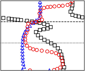
Figure 7 compares the phase discrepancies between  $-({ \textrm {d} T}/{\textrm {d}y})({\hat {v}}/{T})$ and
  $\mathrm {i}(\alpha U-\omega )({\hat {T}}/{T})$ around the critical layer at different frequencies:
  $\omega _1=0.13$,
  $\omega _2=0.152$ and
  $\omega _3=0.17$. The corresponding eigenvalues are
  $\alpha _1=0.1388-0.0005\mathrm {i}$,
  $\alpha _2=0.164-0.004\mathrm {i}$ and
  $\alpha _3=0.1854-0.0019\mathrm {i}$, respectively. It is clear that a smaller phase discrepancy in the vicinity of the critical layer corresponds to a larger growth rate
  $-{\textrm {Im}}(\alpha )$. Again, this is because that when the wall-normal energy transport is in phase with the change of fluctuating internal energy of a finite control volume, it has a positive impact on local perturbations, namely, escalating local perturbations. In contrast, a manifest phase discrepancy between
  $-({ \textrm {d} T}/{\textrm {d}y})({\hat {v}}/{T})$ and
  $\mathrm {i}(\alpha U-\omega )({\hat {T}}/{T})$ gives rise to the occurrence of energy transported by the wall-normal velocity fluctuation being added at the phase when the internal energy decreases, or being taken away at the phase of increasing internal energy, which attenuates local perturbations. That explains why the case
  $\omega _2=0.152$ has the largest growth rate. In turn, the wall-normal fluctuating velocity is accelerated to adapt to the change of the local pressure fluctuation resulting from the increase in internal energy fluctuation.

Figure 7. Phase profiles of  $-({ \textrm {d} T}/{\textrm {d}y})({\hat {v}}/{T})$ and
  $\mathrm {i}(\alpha U-\omega )({\hat {T}}/{T})$ of the cases: (a)
  $\omega _1=0.13$, (b)
  $\omega _2=0.152$ and (c)
  $\omega _3=0.17$, with the corresponding eigenvalues of
  $\alpha _1=0.1388-0.0005\mathrm {i}$,
  $\alpha _2=0.164-0.004\mathrm {i}$ and
  $\alpha _3=0.1854-0.0019\mathrm {i}$, respectively. The dashed line denotes the critical layer.
The relative phase of  $-({ \textrm {d} T}/{\textrm {d}y})({\hat {v}}/{T})$ to
  $\mathrm {i}(\alpha U-\omega )({\hat {T}}/{T})$ in the vicinity of the critical layer is also associated with the near-wall dilatation fluctuation. From figure 6(b), we observe that the phase of the term
  $-({ \textrm {d} T}/{\textrm {d}y})({\hat {v}}/{T})$ is counter to that of the term
  $-(\gamma -1)(\mathrm {i}\alpha \hat {u} + { \textrm {d}\hat {v}}/{\textrm {d}y})$ between the sonic line and the wall. That is, the energy transport by the wall-normal velocity fluctuation (
 $-({ \textrm {d} T}/{\textrm {d}y})({\hat {v}}/{T}$)) is in phase with the rate of energy change due to dilatation fluctuations
  $(\gamma -1)(\mathrm {i}\alpha \hat {u} + { \textrm {d}\hat {v}}/{\textrm {d}y})$. Therefore, the wall-normal transport of energy will intensify the near-wall dilatation fluctuation. Assuming that the internal energy perturbations of these three frequencies have the same intensity at the critical layer, the near-wall dilatation fluctuation of the case
  $\omega _2=0.152$ (among three cases in figure 7) will be of the largest intensity, which is consistent with figure 8. In turn, intensified dilatation fluctuations also accelerate the wall-normal fluctuating velocity, as well as the streamwise fluctuating velocity. Consequently, the near-wall fluctuation mutually interacts with the critical-layer fluctuation, which underpins the growth of second-mode instability.

Figure 8. Distribution of  $|(\gamma -1)(\mathrm {i}\alpha \hat {u}+{ \textrm {d}\hat {v}}/{\textrm {d}y})|$ scaled by the maximum value of
  ${|{-}\,\mathrm {i}\omega ({\hat {T}}/{T})}|$.
4. Stabilization of the second mode
Theoretical and experimental studies have confirmed that porous surfaces that are compatible with the surfaces of thermal protection systems can stabilize second-mode instability (Malmuth et al. Reference Malmuth, Fedorov, Shalaev, Cole, Hites, Williams and Khokhlov1998; Fedorov et al. Reference Fedorov, Malmuth, Rasheed and Hornung2001; Rasheed et al. Reference Rasheed, Hornung, Fedorov and Malmuth2002; Fedorov et al. Reference Fedorov, Shiplyuk, Maslov, Burov and Malmuth2003; Wagner et al. Reference Wagner, Kuhn, Schramm and Hannemann2013). These porous surfaces, consisting of microstructures with the pore size less than approximately  $100\ \mathrm {\mu }$m, do not disrupt the mean flow but are semitransparent for incident waves.
The absorption mechanism of disturbance energy by porous coatings is well perceived to explain the stabilization of the second mode (Malmuth et al. Reference Malmuth, Fedorov, Shalaev, Cole, Hites, Williams and Khokhlov1998; Fedorov et al. Reference Fedorov, Malmuth, Rasheed and Hornung2001). Therefore, a small reflection coefficient is endeavoured for the design of porous coatings. Generally, the minimal reflection coefficient occurs at the admittance phase of  ${\rm \pi}$, namely,
  $A$ is a negative number. Here we employ a porous wall with the admittance of
  $A=-4$. The eigenvalue of the porous-wall case for
  $\omega =0.152$ is
  $\alpha =0.1646-0.00165\mathrm {i}$. Apparently, the growth rate decreases markedly compared with the smooth-solid-wall case, in which
  $-{\textrm {Im}}(\alpha )=0.004$. Figure 9 depicts the amplitude and phase profiles of eigenfunctions of the porous-wall case, and figure 10 shows the amplitude and phase profiles of
  $-(\gamma -1)(\mathrm {i}\alpha \hat {u} + { \textrm {d}\hat {v}}/{\textrm {d}y})$,
  $-({ \textrm {d} T}/{\textrm {d}y})({\hat {v}}/{T})$ and
  $\mathrm {i}(\alpha U-\omega )({\hat {T}}/{T})$.

Figure 9. (a) Amplitude and (b) phase profiles of eigenfunctions of the second mode at  $\omega =0.152$ with
  $\alpha =0.1646-0.00165\mathrm {i}$ in the porous-wall case. The dashed and dotted lines denote the critical layer and the sonic line, respectively.

Figure 10. (a) Amplitude and (b) phase profiles of  $-(\gamma -1)(\mathrm {i}\alpha \hat {u} + { \textrm {d}\hat {v}}/{\textrm {d}y})$,
  $-({ \textrm {d} T}/{\textrm {d}y})({\hat {v}}/{T})$ and
  $\mathrm {i}(\alpha U-\omega )({\hat {T}}/{T})$ for the second mode at
  $\omega =0.152$ with
  $\alpha =0.1646-0.00165\mathrm {i}$ in the porous-wall case. The dashed and dotted lines denote the critical layer and the sonic line, respectively.
By comparing figures 6(b) and 10(b), we observe that the phase of the term  $-({ \textrm {d} T}/{\textrm {d}y})({\hat {v}}/{T})$ against the wall is shifted from
  $0.5{\rm \pi}$ to
  ${\rm \pi}$ as the porous wall is applied. According to the time dependence of
  $\exp (-\mathrm {i}\omega t)$, the phase of
  $-({ \textrm {d} T}/{\textrm {d}y})({\hat {v}}/{T})$ varies from
  $2{\rm \pi}$ to 0 with increasing time; therefore, the wall-normal energy transport is delayed at the wall in the porous-wall case. Moreover, the delay is exerted on the near-wall field due to fluid continuity. Then, the interaction between the near-wall fluctuation and the critical-layer fluctuation via the wall-normal transport of energy is recast. Figure 10(b) shows that the phase of
  $-({ \textrm {d} T}/{\textrm {d}y})({\hat {v}}/{T})$ obviously differs from that of
  $\mathrm {i}(\alpha U-\omega )({\hat {T}}/{T})$ in the region adjacent to the critical layer, which diminishes the positive contribution of energy transport by the wall-normal velocity fluctuation to the internal energy fluctuation and results in a decrease in the growth rate.
5. Conclusions
Theoretical analyses based on the rates of change of perturbations were performed to demonstrate the perturbation regime of second-mode instability in hypersonic boundary layers and to explain the detailed mechanisms of its growth. We have also elucidated the mechanisms of the stabilization effect of porous walls on second-mode instability. The streamwise velocity perturbation is strengthened by the concurrence of the momentum transfer due to the wall-normal velocity fluctuation and the streamwise gradient of the pressure fluctuation near the wall. The wall-normal velocity fluctuation is ruled by the wall-normal gradient of the pressure fluctuation. The internal energy fluctuation is advection-transport-dominated in the vicinity of the critical layer and dilatation-dominated near the wall. The wall-normal velocity fluctuations draw energy from the mean flow to the disturbance field, which results in the growth of second-mode instability. The growth rate of second-mode instability relies on the relative phase of the wall-normal transport of energy to the change of fluctuating internal energy in the vicinity of the critical layer. Moreover, this relative phase is associated with the mutual interaction between the critical-layer fluctuation and the near-wall fluctuation. Porous walls recast this mutual interaction by delaying the phase of the wall-normal energy transport near the wall, thus the energy transferred to the internal energy fluctuation is out of phase with the change of fluctuating internal energy, thus rendering a decrease in the growth rate of second-mode instability.
Generally, porous walls have a destabilization effect on the first mode. To analyse the destabilization of the first mode, we have conducted similar computations based on the same basic flow. Because this paper mainly focuses on second-mode instability, the preliminary analyses on the first mode are included in appendix B. The destabilization effects of the porous wall on the first mode definitely merits further study.
Acknowledgements
This work is supported by the Research Grants Council, Hong Kong, under contract no. C5010-14E and no. 152041/18E, and the National Natural Science Foundation of China under contract no. 11772284 and no. 11872116. The authors acknowledge discussions with Dr R. Zhao, Mr T. Long and Dr J. Hao.
Declaration of interests
The authors report no conflict of interest.
Appendix A. The matrix elements
Non-zero elements of the matrix  $H$ in (2.2) are
 \begin{equation} \left.\begin{gathered} H_{12}=H_{56}=1, \\ H_{21}=\alpha^{2}+\mathrm{i}(\alpha U-\omega)\frac{R}{\mu T},\quad H_{22}=-\frac{1}{\mu}\frac{ \textrm{d}\mu}{\textrm{d}y}, \\ H_{23}=-\mathrm{i}\alpha\left(\frac{1}{3T}\frac{ \textrm{d} T}{\textrm{d}y}+\frac{1}{\mu}\frac{ \textrm{d}\mu}{\textrm{d}y}\right)+\frac{R}{\mu T}\frac{ \textrm{d} U}{\textrm{d}y},\quad H_{24}=\mathrm{i}\alpha\frac{R}{\mu}-\frac{1}{3}\gamma M^{2}_e \alpha(\alpha U-\omega), \\ H_{25}=\frac{1}{3T}\alpha(\alpha U-\omega)-\frac{1}{\mu} \frac{ \textrm{d}}{\textrm{d}y}\left(\frac{ \textrm{d}\mu}{ \textrm{d} T}\frac{ \textrm{d} U}{\textrm{d}y}\right),\quad H_{26}=-\frac{1}{\mu}\frac{ \textrm{d}\mu}{\textrm{d}y}\frac{ \textrm{d} U}{\textrm{d}y} \\ H_{31}=-\mathrm{i}\alpha,\quad H_{33}=\frac{1}{T}\frac{ \textrm{d} T}{\textrm{d}y},\quad H_{34}=-\mathrm{i}\gamma M^{2}_e(\alpha U-\omega),\quad H_{35}=\frac{\mathrm{i}}{T}(\alpha U-\omega), \\ H_{41}=-\mathrm{i}\chi\alpha\left(\frac{4}{3T}\frac{ \textrm{d} T}{\textrm{d}y}+ \frac{2}{\mu}\frac{ \textrm{d}\mu}{\textrm{d}y}\right),\quad H_{42}=-\mathrm{i}\alpha\chi, \\ H_{43}=\chi\left[-\alpha^{2}+\frac{4}{3\mu T}\frac{ \textrm{d}\mu}{\textrm{d}y} \frac{ \textrm{d} T}{\textrm{d}y}+\frac{4}{3T}\frac{ \textrm{d}^{2}T}{{\textrm{d}y}^{2}}- \frac{\mathrm{i}R}{\mu T}(\alpha U-\omega)\right], \\ H_{44}=-\frac{4}{3}\mathrm{i}\chi\gamma M^{2}_e\left[\alpha\frac{ \textrm{d} U}{\textrm{d}y}+ \left(\frac{1}{T}\frac{ \textrm{d} T}{\textrm{d}y}+\frac{1}{\mu}\frac{ \textrm{d}\mu}{\textrm{d}y}\right)(\alpha U-\omega)\right], \\ H_{45}=\mathrm{i}\chi\left[\frac{4}{3}\frac{\alpha}{T}\frac{ \textrm{d} U}{\textrm{d}y}+\frac{\alpha}{\mu}\frac{ \textrm{d}\mu}{ \textrm{d} T}\frac{ \textrm{d} U}{\textrm{d}y}+\frac{4}{3\mu T}\frac{ \textrm{d}\mu}{\textrm{d}y}(\alpha U-\omega)\right],\quad H_{46}=\frac{4\mathrm{i}}{3}\frac{\chi}{T}(\alpha U-\omega), \\ H_{62}=-2{{{Pr}}}(\gamma-1)M^{2}_e\frac{ \textrm{d} U}{\textrm{d}y},\quad H_{63}=\frac{R Pr}{\mu T}\frac{ \textrm{d} T}{\textrm{d}y}-2\mathrm{i}\alpha(\gamma-1)M^{2}_e{{{Pr}}}\frac{ \textrm{d} U}{\textrm{d}y}, \\ H_{64}=-\frac{\mathrm{i}R Pr}{\mu}(\gamma-1)M^{2}_e(\alpha U-\omega),\quad H_{66}=-\frac{2}{\mu}\frac{ \textrm{d}\mu}{\textrm{d}y}, \\ H_{65}=\alpha^{2}+\frac{\mathrm{i}R Pr}{\mu T}(\alpha U-\omega)-(\gamma-1)M^{2}_e\frac{Pr}{\mu}\frac{ \textrm{d}\mu}{ \textrm{d} T} \left(\frac{ \textrm{d} U}{\textrm{d}y}\right)^{2}-\frac{1}{\mu}\frac{ \textrm{d}^{2}\mu}{{\textrm{d}y}^{2}}, \end{gathered}\right\} \end{equation}
where  $\chi =[{R}/{\mu }+\frac {4}{3}\mathrm {i}\gamma M^{2}_e(\alpha U-\omega )]^{-1}$,
  $M_e$ is the Mach number at the boundary-layer edge,
  $U$,
$U$,  $T$ and
  $\mu$ are the mean velocity, temperature and viscosity, respectively,
  $R$,
$R$,  ${{{Pr}}}$ and
  $\gamma$ are the Reynolds number, Prandtl number and specific heat ratio, respectively. Note that Stokes’ hypothesis is employed in the above formulas.
Appendix B. Destabilization of the first mode
To analyse the destabilization of the first mode, we conduct computations based on the same basic flow. Under the current boundary layer, the most unstable first mode occurs at  $\omega =0.063$. In the smooth-solid-wall case (
 $A=0$), the growth rate is
  $-{\textrm {Im}}(\alpha )=0.00039$, while in the porous-wall case with
  $A=-8$, the growth rate is
  $-{\textrm {Im}}(\alpha )=0.00109$. The profiles of eigenfunctions for the solid-wall case and porous-wall case are depicted in figures 11 and 12, respectively. We compare the energy terms between the solid-wall case and porous-wall case, which are depicted in figures 13 and 14, respectively. Apparently, the phase discrepancy between
  $\mathrm {i}(\alpha U-\omega )({\hat {T}}/{T})$ and
  $-({ \textrm {d} T}/{\textrm {d}y})({\hat {v}}/{T})$ in the vicinity of the critical layer is narrowed in the porous-wall case compared with the solid-wall case. Therefore, the destabilization of the first mode is associated with the contribution of energy transport by the wall-normal velocity fluctuation to the internal energy fluctuation. In addition, the phase delay in wall-normal velocity fluctuation caused by the porous wall has different impacts on the critical-layer perturbations between the first and second mode, which merits further study.

Figure 11. (a) Amplitude and (b) phase profiles of eigenfunctions of the first mode at  $\omega =0.063$ with
  $\alpha =0.07068-0.00039\mathrm {i}$ in the smooth-solid-wall case (
 $A=0$). The dashed and dotted lines denote the critical layer and the sonic line, respectively.

Figure 12. (a) Amplitude and (b) phase profiles of eigenfunctions of the first mode at  $\omega =0.063$ with
  $\alpha =0.07066-0.00109\mathrm {i}$ in the porous-wall case (
 $A=-8$). The dashed and dotted lines denote the critical layer and the sonic line, respectively.

Figure 13. (a) Amplitude and (b) phase profiles of  $-(\gamma -1)(\mathrm {i}\alpha \hat {u} + { \textrm {d}\hat {v}}/{\textrm {d} y})$,
  $-({ \textrm {d} T}/{\textrm {d}y})({\hat {v}}/{T})$ and
  $\mathrm {i}(\alpha U-\omega )({\hat {T}}/{T})$ for the first mode at
  $\omega =0.063$ with
  $\alpha =0.07068-0.00039\mathrm {i}$ in the smooth-solid-wall case (
 $A=0$). The dashed and dotted lines denote the critical layer and the sonic line, respectively.

Figure 14. (a) Amplitude and (b) phase profiles of  $-(\gamma -1)(\mathrm {i}\alpha \hat {u} + { \textrm {d}\hat {v}}/{\textrm {d}y})$,
  $-({ \textrm {d} T}/{\textrm {d}y})({\hat {v}}/{T})$ and
  $\mathrm {i}(\alpha U-\omega )({\hat {T}}/{T})$ for the first mode at
  $\omega =0.152$ with
  $\alpha =0.07066-0.00109\mathrm {i}$ in the porous-wall case (
 $A=-8$). The dashed and dotted lines denote the critical layer and the sonic line, respectively.


