


1 Introduction
Directional drilling, and in particular horizontal drilling, has been an important technique in oil and gas extraction since the early twentieth century. During the drilling process, an annular void between the casing string and the drilled hole is created. This void is initially full of a drilling fluid commonly referred to as mud, which is used to cool the drill bit and lubricate the drilling process. Once drilling has been completed, the annulus is filled with cement, which upon curing, will add stability and integrity to the wellbore (Sauer & Till Reference Sauer and Till1987). The time-dependent interaction of the interface between the cement and mud – during the displacement procedure – is crucial in determining the effectiveness of the mud displacement (Eduardo, Dutra & Monica Reference Eduardo, Dutra and Monica2004), and thus the quality of the seal in the well.
Models of the motion of the cement–mud interface typically describe the flow along the well, and often the focus is on the non-uniform gap width, which leads to channelling of the cement along the wider part of the annulus. Typically the annular gap is only 1–3 cm thick, while the radius is 10–15 cm. Furthermore, in many cases the cement is injected for hundreds of metres along the well, so that the interface between the cement and the mud tends to be parallel to the axis of the well, with its position varying slowly along the well. As well as the process of injection of the cement into the well, the late-time adjustment of the cement interface associated with the density differences between the phases is of interest. Given the aspect ratio of the well, an azimuthal gravity-driven flow may develop if the interface between the mud and cement is not horizontal in the cross-annulus plane. There may also be a long-time along-axis flow owing to variations in the depth of the flow along the well. Since the gradient of the interface in the along-axis direction will be small, owing to the long distances travelled by the cement along the well, the slope of the interface in the cross-annulus direction, which arises from the detailed pattern of flow along the annulus, may be dominant, and hence we focus on the gravity-driven flow around the annulus (figure 1). In order to understand the fluid mechanics of such an adjustment flow, we consider the idealised problem in which we neglect the along-axis flow, and explore how the adjustment around the annulus occurs for a range of initial conditions. This class of problem is of interest in itself as it is different from the classical viscous gravity current (Huppert Reference Huppert1982) or viscous exchange flow problems (Matson & Hogg Reference Matson and Hogg2012) as we emphasise in our analysis. While the range of initial conditions we cover may exceed those likely to arise in the drilling problem, the more extensive analysis reported herein leads to insight into the controls on this general class of flows.
In this paper we study this late-time azimuthal adjustment of the cement–mud interface, focusing on the time scale for the flow to relax to a vertically stratified stable regime when initially the interface is inclined. In § 2 we develop the theory, neglecting surface tension effects, such that the contact between the fluid–fluid interface and the annulus walls does not play a role in limiting the current propagation rate (Takagi & Huppert Reference Takagi and Huppert2007). In § 3 several flow regimes are identified and a critical mass condition derived. In §§ 4 and 5 we present numerical and asymptotic solutions to describe the different flow regimes. Finally, we end with a discussion on how the initial cross-sectional distribution of the cement will play an integral role in the quality of the cementing process.
2 Theory

Figure 1. A schematic of the system under consideration.
Consider two viscous incompressible fluids of viscosities
 $\unicode[STIX]{x1D707}_{I},\unicode[STIX]{x1D707}_{O}$
and densities
$\unicode[STIX]{x1D707}_{I},\unicode[STIX]{x1D707}_{O}$
and densities
 $\unicode[STIX]{x1D70C}_{I},\unicode[STIX]{x1D70C}_{O}$
. The fluids are stably stratified in density and viscosity, such that
$\unicode[STIX]{x1D70C}_{I},\unicode[STIX]{x1D70C}_{O}$
. The fluids are stably stratified in density and viscosity, such that
 $\unicode[STIX]{x1D70C}_{I}<\unicode[STIX]{x1D70C}_{O}$
and
$\unicode[STIX]{x1D70C}_{I}<\unicode[STIX]{x1D70C}_{O}$
and
 $\unicode[STIX]{x1D707}_{I}>\unicode[STIX]{x1D707}_{O}$
, and separated by a density interface
$\unicode[STIX]{x1D707}_{I}>\unicode[STIX]{x1D707}_{O}$
, and separated by a density interface
 $h(\unicode[STIX]{x1D703},t)$
. The velocity of each fluid in the azimuthal direction is denoted
$h(\unicode[STIX]{x1D703},t)$
. The velocity of each fluid in the azimuthal direction is denoted
 $u_{I}$
and
$u_{I}$
and
 $u_{O}$
. As shown schematically (figure 1) the domain of interest is a thin annulus of inner radius
$u_{O}$
. As shown schematically (figure 1) the domain of interest is a thin annulus of inner radius
 $R$
and gap width
$R$
and gap width
 $H\ll R$
. We define
$H\ll R$
. We define
 $r$
to be the radial coordinate, as measured from the inner wall, and
$r$
to be the radial coordinate, as measured from the inner wall, and
 $\unicode[STIX]{x1D703}$
to be the azimuthal coordinate, as measured from the base of the annulus. A leading-order expansion of the two-dimensional polar Navier–Stokes equations under the thin-gap approximation leads us to the governing equations of motion,
$\unicode[STIX]{x1D703}$
to be the azimuthal coordinate, as measured from the base of the annulus. A leading-order expansion of the two-dimensional polar Navier–Stokes equations under the thin-gap approximation leads us to the governing equations of motion,
 $$\begin{eqnarray}\frac{\unicode[STIX]{x2202}p}{\unicode[STIX]{x2202}r}=\unicode[STIX]{x1D70C}g\cos \unicode[STIX]{x1D703},\quad \frac{1}{R}\frac{\unicode[STIX]{x2202}p}{\unicode[STIX]{x2202}\unicode[STIX]{x1D703}}=\unicode[STIX]{x1D707}\frac{\unicode[STIX]{x2202}^{2}u}{\unicode[STIX]{x2202}r^{2}}-\unicode[STIX]{x1D70C}g\sin \unicode[STIX]{x1D703},\end{eqnarray}$$
in the radial and azimuthal directions respectively. We can integrate (2.1b
) to obtain equations for the velocities
 $u_{I}$
and
$u_{I}$
and
 $u_{O}$
,
$u_{O}$
,
 $$\begin{eqnarray}\displaystyle & \displaystyle u_{I}=\frac{1}{2\unicode[STIX]{x1D707}_{I}}\left(\frac{1}{R}\frac{\unicode[STIX]{x2202}p}{\unicode[STIX]{x2202}\unicode[STIX]{x1D703}}+\unicode[STIX]{x1D70C}_{I}g\sin \unicode[STIX]{x1D703}\right)r^{2}+C_{1}r+C_{2}, & \displaystyle\end{eqnarray}$$
 $$\begin{eqnarray}\displaystyle & \displaystyle u_{O}=\frac{1}{2\unicode[STIX]{x1D707}_{O}}\left(\frac{1}{R}\frac{\unicode[STIX]{x2202}p}{\unicode[STIX]{x2202}\unicode[STIX]{x1D703}}+\unicode[STIX]{x1D70C}_{O}g\sin \unicode[STIX]{x1D703}\right)r^{2}+C_{3}r+C_{4}. & \displaystyle\end{eqnarray}$$
 $C_{1},C_{2},C_{3}$
and
$C_{1},C_{2},C_{3}$
and
 $C_{4}$
can be calculated with the application of four boundary conditions. Firstly, the speed parallel to the annulus walls is zero. Secondly, the velocity is continuous across the density interface,
$C_{4}$
can be calculated with the application of four boundary conditions. Firstly, the speed parallel to the annulus walls is zero. Secondly, the velocity is continuous across the density interface,
 $r=h$
. Finally, the viscous shear stress is continuous across the density interface. Thus
$r=h$
. Finally, the viscous shear stress is continuous across the density interface. Thus  $$\begin{eqnarray}u_{I}(0)=u_{O}(H)=0,\quad u_{I}(h)=u_{O}(h),\quad \unicode[STIX]{x1D707}_{I}\frac{\unicode[STIX]{x2202}u_{I}}{\unicode[STIX]{x2202}r}(h)=\unicode[STIX]{x1D707}_{O}\frac{\unicode[STIX]{x2202}u_{O}}{\unicode[STIX]{x2202}r}(h).\end{eqnarray}$$
Equation (2.1a
) represents the approximation that the pressure
 $p$
in the radial direction varies hydrostatically, with
$p$
in the radial direction varies hydrostatically, with
 $$\begin{eqnarray}p(r,\unicode[STIX]{x1D703})=\left\{\begin{array}{@{}ll@{}}\displaystyle p_{0}(\unicode[STIX]{x1D703})+\unicode[STIX]{x1D70C}_{I}gr\cos \unicode[STIX]{x1D703} & \text{if}~0\leqslant r\leqslant h,\\ \displaystyle p_{0}(\unicode[STIX]{x1D703})+\unicode[STIX]{x1D70C}_{I}gh\cos \unicode[STIX]{x1D703}+\unicode[STIX]{x1D70C}_{O}g(r-h)\cos \unicode[STIX]{x1D703} & \text{if}~h\leqslant r\leqslant H,\end{array}\right.\end{eqnarray}$$
and where
 $p_{0}(\unicode[STIX]{x1D703})$
is the unknown pressure on the inner wall. We substitute (2.4) into (2.2a
) and (2.2b
), discarding any terms of
$p_{0}(\unicode[STIX]{x1D703})$
is the unknown pressure on the inner wall. We substitute (2.4) into (2.2a
) and (2.2b
), discarding any terms of
 $O(R^{-1})$
, to obtain a pair of equations for
$O(R^{-1})$
, to obtain a pair of equations for
 $u_{I}$
and
$u_{I}$
and
 $u_{O}$
in terms of the unknown pressure gradient
$u_{O}$
in terms of the unknown pressure gradient
 $p_{0_{\unicode[STIX]{x1D703}}}$
and interfacial functions
$p_{0_{\unicode[STIX]{x1D703}}}$
and interfacial functions
 $h$
and
$h$
and
 $h_{\unicode[STIX]{x1D703}}$
. To obtain expressions for
$h_{\unicode[STIX]{x1D703}}$
. To obtain expressions for
 $p_{0_{\unicode[STIX]{x1D703}}}$
and
$p_{0_{\unicode[STIX]{x1D703}}}$
and
 $h_{\unicode[STIX]{x1D703}}$
, we assume that there is no net flux,
$h_{\unicode[STIX]{x1D703}}$
, we assume that there is no net flux,
 $$\begin{eqnarray}\int _{0}^{h}u_{I}\,\text{d}r=-\int _{h}^{H}u_{O}\,\text{d}r.\end{eqnarray}$$
Finally, we can use the global continuity equation (Acheson Reference Acheson1990)
 $$\begin{eqnarray}\frac{\unicode[STIX]{x2202}h}{\unicode[STIX]{x2202}t}+\frac{1}{R}\frac{\unicode[STIX]{x2202}}{\unicode[STIX]{x2202}\unicode[STIX]{x1D703}}\left(\int _{0}^{h}u_{I}\,\text{d}r\right)=0,\end{eqnarray}$$
to obtain a partial differential equation that describes the movement in time and space of the density interface
 $h(\unicode[STIX]{x1D703},t)$
:
$h(\unicode[STIX]{x1D703},t)$
:
 $$\begin{eqnarray}\frac{\unicode[STIX]{x2202}h}{\unicode[STIX]{x2202}t}+\frac{\unicode[STIX]{x0394}\unicode[STIX]{x1D70C}g}{3R^{2}}\frac{\unicode[STIX]{x2202}}{\unicode[STIX]{x2202}\unicode[STIX]{x1D703}}\left[\frac{h^{3}(H-h)^{3}(H\unicode[STIX]{x1D707}_{I}-\unicode[STIX]{x0394}\unicode[STIX]{x1D707}h)\left((h+R)\sin \unicode[STIX]{x1D703}-{\displaystyle \frac{\unicode[STIX]{x2202}h}{\unicode[STIX]{x2202}\unicode[STIX]{x1D703}}}\cos \unicode[STIX]{x1D703}\right)}{H^{4}\unicode[STIX]{x1D707}_{I}^{2}-4H^{3}\unicode[STIX]{x1D707}_{I}\unicode[STIX]{x0394}\unicode[STIX]{x1D707}h+6H^{2}\unicode[STIX]{x1D707}_{I}\unicode[STIX]{x0394}\unicode[STIX]{x1D707}h^{2}-4H\unicode[STIX]{x1D707}_{I}\unicode[STIX]{x0394}\unicode[STIX]{x1D707}h^{3}+\unicode[STIX]{x0394}\unicode[STIX]{x1D707}^{2}h^{4}}\right]=0,\end{eqnarray}$$
where
 $\unicode[STIX]{x0394}\unicode[STIX]{x1D70C}=\unicode[STIX]{x1D70C}_{O}-\unicode[STIX]{x1D70C}_{I}$
and
$\unicode[STIX]{x0394}\unicode[STIX]{x1D70C}=\unicode[STIX]{x1D70C}_{O}-\unicode[STIX]{x1D70C}_{I}$
and
 $\unicode[STIX]{x0394}\unicode[STIX]{x1D707}=\unicode[STIX]{x1D707}_{I}-\unicode[STIX]{x1D707}_{O}$
. This equation lends itself to the following scalings:
$\unicode[STIX]{x0394}\unicode[STIX]{x1D707}=\unicode[STIX]{x1D707}_{I}-\unicode[STIX]{x1D707}_{O}$
. This equation lends itself to the following scalings:
 $$\begin{eqnarray}h=H{\hat{h}},\quad t=\frac{3R\unicode[STIX]{x1D707}_{I}}{\unicode[STIX]{x0394}\unicode[STIX]{x1D70C}gH^{2}}\hat{t},\quad \unicode[STIX]{x1D700}=\frac{H}{R},\quad \unicode[STIX]{x0394}\hat{\unicode[STIX]{x1D707}}=\frac{\unicode[STIX]{x0394}\unicode[STIX]{x1D707}}{\unicode[STIX]{x1D707}_{I}},\end{eqnarray}$$
where
 $\unicode[STIX]{x1D700}$
is a small parameter. Henceforth, for convenience we drop the hat notation and obtain the non-dimensional equation of motion:
$\unicode[STIX]{x1D700}$
is a small parameter. Henceforth, for convenience we drop the hat notation and obtain the non-dimensional equation of motion:
 $$\begin{eqnarray}\frac{\unicode[STIX]{x2202}h}{\unicode[STIX]{x2202}t}+\frac{\unicode[STIX]{x2202}}{\unicode[STIX]{x2202}\unicode[STIX]{x1D703}}\left[\frac{h^{3}(1-h)^{3}(1-\unicode[STIX]{x0394}\unicode[STIX]{x1D707}h)\left((1+\unicode[STIX]{x1D700})\sin \unicode[STIX]{x1D703}-\unicode[STIX]{x1D700}{\displaystyle \frac{\unicode[STIX]{x2202}h}{\unicode[STIX]{x2202}\unicode[STIX]{x1D703}}}\cos \unicode[STIX]{x1D703}\right)}{1-4\unicode[STIX]{x0394}\unicode[STIX]{x1D707}h+6\unicode[STIX]{x0394}\unicode[STIX]{x1D707}h^{2}-4\unicode[STIX]{x0394}\unicode[STIX]{x1D707}h^{3}+\unicode[STIX]{x0394}\unicode[STIX]{x1D707}^{2}h^{4}}\right]=0.\end{eqnarray}$$
Data from studies on the rheology of typical drilling lubricant (Kudaikulova Reference Kudaikulova2015) and oil well cement (Shahriar Reference Shahriar2011) suggest that a viscosity difference
 $\unicode[STIX]{x0394}\unicode[STIX]{x1D707}\ll 1$
is a good approximation. The cement and lubrication mud used in the drilling process are known to be non-Newtonian; however, for the range of shear rates we expect in this study, a Newtonian approximation should accurately describe the
$\unicode[STIX]{x0394}\unicode[STIX]{x1D707}\ll 1$
is a good approximation. The cement and lubrication mud used in the drilling process are known to be non-Newtonian; however, for the range of shear rates we expect in this study, a Newtonian approximation should accurately describe the
 $O(1)$
behaviour. In the limit that we take the viscosity of the two fluids to be the same, we can reduce (2.9) to the simplified version, which we will consider for the rest of this paper:
$O(1)$
behaviour. In the limit that we take the viscosity of the two fluids to be the same, we can reduce (2.9) to the simplified version, which we will consider for the rest of this paper:
 $$\begin{eqnarray}\frac{\unicode[STIX]{x2202}h}{\unicode[STIX]{x2202}t}+\frac{\unicode[STIX]{x2202}}{\unicode[STIX]{x2202}\unicode[STIX]{x1D703}}\left[h^{3}(1-h)^{3}\left((1+\unicode[STIX]{x1D700}h)\sin \unicode[STIX]{x1D703}-\unicode[STIX]{x1D700}\frac{\unicode[STIX]{x2202}h}{\unicode[STIX]{x2202}\unicode[STIX]{x1D703}}\cos \unicode[STIX]{x1D703}\right)\right]=0.\end{eqnarray}$$
If the azimuthal coordinate
 $\unicode[STIX]{x1D703}$
is constant, (2.10) would in fact describe a gravity current or exchange flow associated with two fluids of different density confined within an inclined channel of finite depth. An analogous equation was presented by Gunn & Woods (Reference Gunn and Woods2011) for flow in an inclined confined porous channel. The two key differences in the present problem are that the azimuthal coordinate
$\unicode[STIX]{x1D703}$
is constant, (2.10) would in fact describe a gravity current or exchange flow associated with two fluids of different density confined within an inclined channel of finite depth. An analogous equation was presented by Gunn & Woods (Reference Gunn and Woods2011) for flow in an inclined confined porous channel. The two key differences in the present problem are that the azimuthal coordinate
 $\unicode[STIX]{x1D703}$
varies with position along the channel owing to the curvature and that this is a pure fluid rather than flow in a porous medium. The term proportional to
$\unicode[STIX]{x1D703}$
varies with position along the channel owing to the curvature and that this is a pure fluid rather than flow in a porous medium. The term proportional to
 $\sin \unicode[STIX]{x1D703}$
corresponds to the effect of the along-boundary component of gravity, which is advective in character, whereas the term proportional to
$\sin \unicode[STIX]{x1D703}$
corresponds to the effect of the along-boundary component of gravity, which is advective in character, whereas the term proportional to
 $\cos \unicode[STIX]{x1D703}$
corresponds to the component normal to the boundary and is diffusive in character.
$\cos \unicode[STIX]{x1D703}$
corresponds to the component normal to the boundary and is diffusive in character.
We note that following a similar shallow-water analysis, the effects of surface tension would lead to an additional pressure gradient of the form
 $\unicode[STIX]{x1D70E}h_{\unicode[STIX]{x1D703}\unicode[STIX]{x1D703}\unicode[STIX]{x1D703}}$
(Myers Reference Myers1998) in addition to the term
$\unicode[STIX]{x1D70E}h_{\unicode[STIX]{x1D703}\unicode[STIX]{x1D703}\unicode[STIX]{x1D703}}$
(Myers Reference Myers1998) in addition to the term
 $\unicode[STIX]{x0394}\unicode[STIX]{x1D70C}gh_{\unicode[STIX]{x1D703}}$
arising from the buoyancy: the surface tension effect only dominates the buoyancy force if the length scale of the flow
$\unicode[STIX]{x0394}\unicode[STIX]{x1D70C}gh_{\unicode[STIX]{x1D703}}$
arising from the buoyancy: the surface tension effect only dominates the buoyancy force if the length scale of the flow
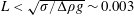 $L<\sqrt{\unicode[STIX]{x1D70E}/\unicode[STIX]{x0394}\unicode[STIX]{x1D70C}g}\sim 0.003$
m. This is smaller than the typical length scales of 0.1–1.0 m of interest in the present problem, and hence we do not include it in the present analysis.
$L<\sqrt{\unicode[STIX]{x1D70E}/\unicode[STIX]{x0394}\unicode[STIX]{x1D70C}g}\sim 0.003$
m. This is smaller than the typical length scales of 0.1–1.0 m of interest in the present problem, and hence we do not include it in the present analysis.
3 Regimes

Figure 2. Steady-state solutions of varying initial volumes
 ${\mathcal{V}}$
of dense fluid in physical space and
${\mathcal{V}}$
of dense fluid in physical space and
 $(1-h,\unicode[STIX]{x1D703})$
space, corresponding to (a) the small-volume case
$(1-h,\unicode[STIX]{x1D703})$
space, corresponding to (a) the small-volume case
 ${\mathcal{V}}<{\mathcal{V}}_{crit}$
, (b) the critical case
${\mathcal{V}}<{\mathcal{V}}_{crit}$
, (b) the critical case
 ${\mathcal{V}}={\mathcal{V}}_{crit}$
, and (c) the large-volume case
${\mathcal{V}}={\mathcal{V}}_{crit}$
, and (c) the large-volume case
 ${\mathcal{V}}>{\mathcal{V}}_{crit}$
.
${\mathcal{V}}>{\mathcal{V}}_{crit}$
.
The final steady-state distribution of the cement and mud involves the interface between the relatively dense cement and the mud being horizontal. The geometry of the annulus leads to two different regimes. With a small volume of cement (per unit length along the axis) relative to the volume of the annulus (per unit length along the axis), the interface will be close to the base of the annulus and will not intersect the inner cylinder (figure 2 a). However, with a larger mass of cement, the interface will intersect the inner cylinder, leading to two spatially separate interfaces on each side of the annulus (figure 2 c). The critical volume of cement at which the interface just touches the inner cylinder (shown in figure 2 b) can be found using the geometry of the problem. The dimensionless volume of cement is given by
 $$\begin{eqnarray}{\mathcal{V}}(\unicode[STIX]{x1D703},\unicode[STIX]{x1D700})=\frac{\displaystyle R\int _{-\unicode[STIX]{x03C0}/2}^{\unicode[STIX]{x03C0}/2}R+H-h(\unicode[STIX]{x1D703})\,\text{d}\unicode[STIX]{x1D703}}{\displaystyle R\int _{-\unicode[STIX]{x03C0}/2}^{\unicode[STIX]{x03C0}/2}H\,\text{d}\unicode[STIX]{x1D703}}=\frac{\displaystyle \int _{-\unicode[STIX]{x03C0}/2}^{\unicode[STIX]{x03C0}/2}1+\unicode[STIX]{x1D700}-\unicode[STIX]{x1D700}h(\unicode[STIX]{x1D703})\,\text{d}\unicode[STIX]{x1D703}}{\displaystyle \int _{-\unicode[STIX]{x03C0}/2}^{\unicode[STIX]{x03C0}/2}\unicode[STIX]{x1D700}\,\text{d}\unicode[STIX]{x1D703}},\end{eqnarray}$$
recalling from (2.8c
) that
 $\unicode[STIX]{x1D700}$
is the non-dimensional gap width and also noting that, because of the approximation
$\unicode[STIX]{x1D700}$
is the non-dimensional gap width and also noting that, because of the approximation
 $\unicode[STIX]{x1D700}\ll 1$
in the theoretical development, we do not need to consider the integral to be polar. Using the coordinate system shown in figure 1, steady-state solutions with a horizontal interface are given by
$\unicode[STIX]{x1D700}\ll 1$
in the theoretical development, we do not need to consider the integral to be polar. Using the coordinate system shown in figure 1, steady-state solutions with a horizontal interface are given by
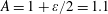
 $$\begin{eqnarray}h(\unicode[STIX]{x1D703})=A\sec \unicode[STIX]{x1D703},\end{eqnarray}$$
with
 $A\in [0,1+\unicode[STIX]{x1D700}]$
. For each value of
$A\in [0,1+\unicode[STIX]{x1D700}]$
. For each value of
 $A$
there is a corresponding initial volume
$A$
there is a corresponding initial volume
 ${\mathcal{V}}$
. By writing the dimensionless volume in this way, it is clear that the critical volume
${\mathcal{V}}$
. By writing the dimensionless volume in this way, it is clear that the critical volume
 ${\mathcal{V}}_{crit}$
corresponds to
${\mathcal{V}}_{crit}$
corresponds to
 $A_{crit}=1$
. In figure 3(a) we plot
$A_{crit}=1$
. In figure 3(a) we plot
 ${\mathcal{V}}(A)$
as a function of
${\mathcal{V}}(A)$
as a function of
 $A$
for four values of
$A$
for four values of
 $\unicode[STIX]{x1D700}$
(0.05, 0.1, 0.2, 0.5). The dotted line at
$\unicode[STIX]{x1D700}$
(0.05, 0.1, 0.2, 0.5). The dotted line at
 $A=1$
illustrates the demarcation between the two regimes. For
$A=1$
illustrates the demarcation between the two regimes. For
 $A>A_{crit}$
, there is a single horizontal interface, and for
$A>A_{crit}$
, there is a single horizontal interface, and for
 $A<A_{crit}$
the interface is piecewise continuous. Equation (3.1) at
$A<A_{crit}$
the interface is piecewise continuous. Equation (3.1) at
 $A=A_{crit}$
can be solved to give an exact expression
$A=A_{crit}$
can be solved to give an exact expression
 $$\begin{eqnarray}{\mathcal{V}}_{crit}=\frac{(1+\unicode[STIX]{x1D700})\sec ^{-1}(1+\unicode[STIX]{x1D700})-\cosh ^{-1}(1+\unicode[STIX]{x1D700})}{\unicode[STIX]{x03C0}\unicode[STIX]{x1D700}},\end{eqnarray}$$
for the critical dimensionless volume. Figure 3(b) illustrates how the critical volume varies as a function of
 $\unicode[STIX]{x1D700}$
. We now explore the transition to these steady states, for the cases of
$\unicode[STIX]{x1D700}$
. We now explore the transition to these steady states, for the cases of
 ${\mathcal{V}}<{\mathcal{V}}_{crit}$
, the small-volume case, and
${\mathcal{V}}<{\mathcal{V}}_{crit}$
, the small-volume case, and
 ${\mathcal{V}}>{\mathcal{V}}_{crit}$
the large-volume case. There are many different possible initial conditions, but in order to gain a systematic understanding of the process of adjustment to equilibrium, we have parametrised the initial condition in terms of a series of partial concentric annuli, which we parametrise as
${\mathcal{V}}>{\mathcal{V}}_{crit}$
the large-volume case. There are many different possible initial conditions, but in order to gain a systematic understanding of the process of adjustment to equilibrium, we have parametrised the initial condition in terms of a series of partial concentric annuli, which we parametrise as
 $h(\unicode[STIX]{x1D703})=h_{0}$
(const.) for
$h(\unicode[STIX]{x1D703})=h_{0}$
(const.) for
 $-\unicode[STIX]{x1D703}_{init}<\unicode[STIX]{x1D703}<\unicode[STIX]{x1D703}_{init}$
. We also define the angle where the interface meets the outer annulus wall at steady state as
$-\unicode[STIX]{x1D703}_{init}<\unicode[STIX]{x1D703}<\unicode[STIX]{x1D703}_{init}$
. We also define the angle where the interface meets the outer annulus wall at steady state as
 $\unicode[STIX]{x1D703}_{steady}$
. An illustration of
$\unicode[STIX]{x1D703}_{steady}$
. An illustration of
 $\unicode[STIX]{x1D703}_{init}$
and
$\unicode[STIX]{x1D703}_{init}$
and
 $\unicode[STIX]{x1D703}_{steady}$
can be seen in figures 4(a) and 4(f) respectively.
$\unicode[STIX]{x1D703}_{steady}$
can be seen in figures 4(a) and 4(f) respectively.

Figure 3. (a) Illustration of how dimensionless mass
 ${\mathcal{V}}$
varies as a function of
${\mathcal{V}}$
varies as a function of
 $A$
, the coefficient of
$A$
, the coefficient of
 $\sec \unicode[STIX]{x1D703}$
that defines straight-line steady states in our coordinate system. The dashed line at
$\sec \unicode[STIX]{x1D703}$
that defines straight-line steady states in our coordinate system. The dashed line at
 $A_{crit}=1$
separates the small-volume and large-volume regimes. In the small-volume regime there is a single steady-state interface. In the large-volume regime we have a piecewise interface that intersects the inner cylinder. (b) Plot showing how
$A_{crit}=1$
separates the small-volume and large-volume regimes. In the small-volume regime there is a single steady-state interface. In the large-volume regime we have a piecewise interface that intersects the inner cylinder. (b) Plot showing how
 $V_{crit}$
varies as a function of the non-dimensional gap width
$V_{crit}$
varies as a function of the non-dimensional gap width
 $\unicode[STIX]{x1D700}$
.
$\unicode[STIX]{x1D700}$
.
To simulate the evolution of the density interface
 $h(\unicode[STIX]{x1D703},t)$
, we have solved (2.10) using a forward-time central-space finite difference method (Ames Reference Ames2014). There are two spatial derivatives, and so we require two spatial boundary conditions. The natural choice for these boundary conditions is that the distal ends of the interface remain on the outer wall of the domain. To ensure the accuracy of the numerical solutions, we tested a number of spatial grid points
$h(\unicode[STIX]{x1D703},t)$
, we have solved (2.10) using a forward-time central-space finite difference method (Ames Reference Ames2014). There are two spatial derivatives, and so we require two spatial boundary conditions. The natural choice for these boundary conditions is that the distal ends of the interface remain on the outer wall of the domain. To ensure the accuracy of the numerical solutions, we tested a number of spatial grid points
 $n=200$
, 500, 1000 and 2000. We found that, as we increased the number of points, the adjustment time required to reach equilibrium converged to constant values, with the difference in this adjustment time between a grid with
$n=200$
, 500, 1000 and 2000. We found that, as we increased the number of points, the adjustment time required to reach equilibrium converged to constant values, with the difference in this adjustment time between a grid with
 $n=1000$
spatial points and
$n=1000$
spatial points and
 $n=2000$
points being less than 0.1 % in all simulations. Furthermore, to check the validity of our numerical scheme, we check for conservation of volume at each time step. For each simulation, the difference between the initial and final volumes was smaller than 1 %. We also ensured the stability of our solution by choosing an appropriate time step for each grid size such that the Courant–Friedrichs–Lewy (CFL) condition
$n=2000$
points being less than 0.1 % in all simulations. Furthermore, to check the validity of our numerical scheme, we check for conservation of volume at each time step. For each simulation, the difference between the initial and final volumes was smaller than 1 %. We also ensured the stability of our solution by choosing an appropriate time step for each grid size such that the Courant–Friedrichs–Lewy (CFL) condition
 $h\unicode[STIX]{x0394}t/\unicode[STIX]{x0394}x<1$
is satisfied.
$h\unicode[STIX]{x0394}t/\unicode[STIX]{x0394}x<1$
is satisfied.
4 Small volume
 $({\mathcal{V}}<{\mathcal{V}}_{crit})$

To analyse the small-volume case, we will first fix
 $\unicode[STIX]{x1D700}=0.2$
such that the gap width is sufficiently small for the flow to be approximately one-dimensional. From (3.3)
$\unicode[STIX]{x1D700}=0.2$
such that the gap width is sufficiently small for the flow to be approximately one-dimensional. From (3.3)
 $\unicode[STIX]{x1D700}=0.2$
gives
$\unicode[STIX]{x1D700}=0.2$
gives
 ${\mathcal{V}}_{crit}\approx 0.128$
. Furthermore, from § 3 we know that each horizontal steady-state interface has a corresponding value of
${\mathcal{V}}_{crit}\approx 0.128$
. Furthermore, from § 3 we know that each horizontal steady-state interface has a corresponding value of
 $A$
. Suppose, at steady state, we wish the fluid to fill half the gap width at
$A$
. Suppose, at steady state, we wish the fluid to fill half the gap width at
 $\unicode[STIX]{x1D703}=0$
. This would correspond to
$\unicode[STIX]{x1D703}=0$
. This would correspond to
 $A=1+\unicode[STIX]{x1D700}/2=1.1$
. Thus (3.1) with
$A=1+\unicode[STIX]{x1D700}/2=1.1$
. Thus (3.1) with
 $h(\unicode[STIX]{x1D703})=1.1\sec \unicode[STIX]{x1D703}$
gives
$h(\unicode[STIX]{x1D703})=1.1\sec \unicode[STIX]{x1D703}$
gives
 ${\mathcal{V}}\approx 0.089$
and
${\mathcal{V}}\approx 0.089$
and
 $\unicode[STIX]{x1D703}_{steady}\approx 0.411$
.
$\unicode[STIX]{x1D703}_{steady}\approx 0.411$
.
4.1 Exchange flow
The first partial concentric annulus we select as an initial condition is
 $h_{0}=0$
. This gives us an initial distribution of fluid that is in contact with the upper boundary of the annulus. For our choice of
$h_{0}=0$
. This gives us an initial distribution of fluid that is in contact with the upper boundary of the annulus. For our choice of
 ${\mathcal{V}}$
we arrive at
${\mathcal{V}}$
we arrive at
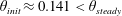 $\unicode[STIX]{x1D703}_{init}\approx 0.141<\unicode[STIX]{x1D703}_{steady}$
. A time series of the interface shape as predicted by the numerical solutions is shown in figure 4. There are three distinct periods of adjustment from the initial condition to the steady state. Firstly, there is an exchange flow occurring between the dense fluid
$\unicode[STIX]{x1D703}_{init}\approx 0.141<\unicode[STIX]{x1D703}_{steady}$
. A time series of the interface shape as predicted by the numerical solutions is shown in figure 4. There are three distinct periods of adjustment from the initial condition to the steady state. Firstly, there is an exchange flow occurring between the dense fluid
 $\unicode[STIX]{x1D70C}_{O}$
and light fluid
$\unicode[STIX]{x1D70C}_{O}$
and light fluid
 $\unicode[STIX]{x1D70C}_{I}$
(figures 4
a,b). A short time later the interface pinches from the inner annulus wall (figure 4
c) and relaxes. The final period of flow is an equilibration to the steady state (figures 4
d–f).
$\unicode[STIX]{x1D70C}_{I}$
(figures 4
a,b). A short time later the interface pinches from the inner annulus wall (figure 4
c) and relaxes. The final period of flow is an equilibration to the steady state (figures 4
d–f).
We note that the detailed process of pinch-off leads to a short period of time during which the radius of curvature of the interface decreases to very small values, although before and after this short interval, the radius of curvature has much larger values (figure 4 a–c). During the pinch-off, the effects of surface tension may therefore become important, limiting the decrease in the radius of curvature at the point at which the interface detaches from the upper boundary. However, this does not have a significant influence on the overall time of relaxation of the interface towards the final steady state. This may be understood by observing that the pinch-off time in the present calculations represents a negligible fraction of the total relaxation time (figure 4 c,d), and the effect of surface tension will be to accelerate the pinch-off, and so we have not included the detail of this in the present calculation.

Figure 4. Results for
 $\unicode[STIX]{x1D703}_{init}\approx 0.141$
. Each panel corresponds to different parts of the flow evolution at various times
$\unicode[STIX]{x1D703}_{init}\approx 0.141$
. Each panel corresponds to different parts of the flow evolution at various times
 $t$
. (a) The initial state, (b) dense and light fluids exchanging, (c) pinch-off of the interface, (d) relaxation, (e) equilibration and (f) steady state.
$t$
. (a) The initial state, (b) dense and light fluids exchanging, (c) pinch-off of the interface, (d) relaxation, (e) equilibration and (f) steady state.

Figure 5. (a) A series of snapshots in time
 $t=0$
, 2, 7.5 and 150. The two currents start off with the same initial condition, but the curvature can be seen to affect the flow of the annular gravity current, bringing it to a stop in finite time with
$t=0$
, 2, 7.5 and 150. The two currents start off with the same initial condition, but the curvature can be seen to affect the flow of the annular gravity current, bringing it to a stop in finite time with
 $h(0)\rightarrow 0.5$
. The classical current flows for an infinite time with
$h(0)\rightarrow 0.5$
. The classical current flows for an infinite time with
 $h(0)\rightarrow 0$
. (b) A demonstration of how the quantity
$h(0)\rightarrow 0$
. (b) A demonstration of how the quantity
 ${\mathcal{E}}$
changes as a function of
${\mathcal{E}}$
changes as a function of
 $t$
. The cross marks the time at which the classical exchange flow separates from the top boundary.
$t$
. The cross marks the time at which the classical exchange flow separates from the top boundary.
In order to illustrate the key impact of the curvature of the boundary on the flow, and the establishment of a steady state, we have compared the numerical solution for annular exchange flow with the case of two fluids of differing density exchanging in a purely horizontal channel, with the same initial conditions. In this case,
 $\unicode[STIX]{x1D703}$
represents the along-channel coordinate. In figure 5(a) profiles of the interface are shown at three times with solid black lines for the annulus and dashed lines for the flat channel. It is seen that, during the initial phase of the flow, while the dense fluid remains attached to the upper boundary of the domain, the flow resembles a classical exchange flow, and the effect of the curvature slows the rate of exchange between the two fluids (figure 5
a,
$\unicode[STIX]{x1D703}$
represents the along-channel coordinate. In figure 5(a) profiles of the interface are shown at three times with solid black lines for the annulus and dashed lines for the flat channel. It is seen that, during the initial phase of the flow, while the dense fluid remains attached to the upper boundary of the domain, the flow resembles a classical exchange flow, and the effect of the curvature slows the rate of exchange between the two fluids (figure 5
a,
 $t=2$
). However, once the fluid separates from the upper boundary (
$t=2$
). However, once the fluid separates from the upper boundary (
 $t=7.5$
), the difference between the solutions becomes more striking, with the fluid adjusting to the steady solution
$t=7.5$
), the difference between the solutions becomes more striking, with the fluid adjusting to the steady solution
 $h=A\sec \unicode[STIX]{x1D703}$
in the annulus, while the fluid adjusts to a classical gravity current in a confined horizontal channel (Huppert Reference Huppert1982; Matson & Hogg Reference Matson and Hogg2012; Zheng, Rongy & Stone Reference Zheng, Rongy and Stone2015). In order to illustrate this difference, it is useful to follow the evolution of the quantity
$h=A\sec \unicode[STIX]{x1D703}$
in the annulus, while the fluid adjusts to a classical gravity current in a confined horizontal channel (Huppert Reference Huppert1982; Matson & Hogg Reference Matson and Hogg2012; Zheng, Rongy & Stone Reference Zheng, Rongy and Stone2015). In order to illustrate this difference, it is useful to follow the evolution of the quantity
 $$\begin{eqnarray}{\mathcal{E}}(t)=\int _{-\unicode[STIX]{x03C0}/2}^{\unicode[STIX]{x03C0}/2}[h_{classical}(\unicode[STIX]{x1D703},t)-h_{annulus}(\unicode[STIX]{x1D703},t)]^{2}\,\text{d}\unicode[STIX]{x1D703},\end{eqnarray}$$
as shown in figure 5(b). The cross on the curve corresponds to the time at which the classical exchange flow separates from the upper boundary.
4.2 Gravity-current-like case

Figure 6. Results for
 $\unicode[STIX]{x1D703}_{init}\approx 0.201$
. Each panel corresponds to different parts of the flow evolution at various times
$\unicode[STIX]{x1D703}_{init}\approx 0.201$
. Each panel corresponds to different parts of the flow evolution at various times
 $t$
. (a) The initial state, (b) the dense fluid begins to slump, (c) the fluid spreads and begins to equilibrate and (d) steady state.
$t$
. (a) The initial state, (b) the dense fluid begins to slump, (c) the fluid spreads and begins to equilibrate and (d) steady state.

Figure 7. (a) A series of snapshots in time
 $t=0$
, 0.5, 5 and 50. The two currents start off with the same initial condition, but the curvature can be seen to affect the flow of the annular gravity current, bringing it to a stop in finite time with
$t=0$
, 0.5, 5 and 50. The two currents start off with the same initial condition, but the curvature can be seen to affect the flow of the annular gravity current, bringing it to a stop in finite time with
 $h(0)\rightarrow 0.5$
. The classical current flows for an infinite time with
$h(0)\rightarrow 0.5$
. The classical current flows for an infinite time with
 $h(0)\rightarrow 0$
. (b) A demonstration of how the quantity
$h(0)\rightarrow 0$
. (b) A demonstration of how the quantity
 ${\mathcal{E}}$
changes as a function of
${\mathcal{E}}$
changes as a function of
 $t$
.
$t$
.
We can explore a further initial condition in the
 $\unicode[STIX]{x1D703}_{init}<\unicode[STIX]{x1D703}_{steady}$
regime by selecting a partial concentric annulus of
$\unicode[STIX]{x1D703}_{init}<\unicode[STIX]{x1D703}_{steady}$
regime by selecting a partial concentric annulus of
 $h_{0}=0.3$
, which leads to
$h_{0}=0.3$
, which leads to
 $\unicode[STIX]{x1D703}_{init}\approx 0.201$
. This condition differs qualitatively from the previous solution shown in § 4.1, as the dense fluid is not in contact with the upper annulus boundary. A visualisation of the full numerical simulation is seen in figure 6. In this case the flow initially behaves analogously to a classical gravity current. At first there is a slumping regime with the dense fluid running along the lower boundary; however, in the annular case the curvature of the domain begins to restrict the flow (figures 6
a,b), as the along-boundary component of gravity suppresses the flow (figures 6
c,d). Eventually the annular current stops flowing and is brought to a horizontal steady state. The disparity between the classical gravity current and the present annular flow can be seen in figure 7(a), with
$\unicode[STIX]{x1D703}_{init}\approx 0.201$
. This condition differs qualitatively from the previous solution shown in § 4.1, as the dense fluid is not in contact with the upper annulus boundary. A visualisation of the full numerical simulation is seen in figure 6. In this case the flow initially behaves analogously to a classical gravity current. At first there is a slumping regime with the dense fluid running along the lower boundary; however, in the annular case the curvature of the domain begins to restrict the flow (figures 6
a,b), as the along-boundary component of gravity suppresses the flow (figures 6
c,d). Eventually the annular current stops flowing and is brought to a horizontal steady state. The disparity between the classical gravity current and the present annular flow can be seen in figure 7(a), with
 $\unicode[STIX]{x1D703}$
again representing the along-channel coordinate for the classical case. The difference function
$\unicode[STIX]{x1D703}$
again representing the along-channel coordinate for the classical case. The difference function
 ${\mathcal{E}}$
(4.1) is again calculated for this gravity-current-like case and shown in figure 7(b).
${\mathcal{E}}$
(4.1) is again calculated for this gravity-current-like case and shown in figure 7(b).
4.3 Draining
By choosing a partial concentric annulus with initial depth
 $h_{0}=0.8$
, we enter a regime where
$h_{0}=0.8$
, we enter a regime where
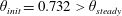 $\unicode[STIX]{x1D703}_{init}=0.732>\unicode[STIX]{x1D703}_{steady}$
. In this case the flow exhibits draining-like behaviour. Dense fluid runs down the outer annulus wall, filling from the base. Figure 8 shows a visualisation of the numerical simulation. In the simulation a thin film develops between
$\unicode[STIX]{x1D703}_{init}=0.732>\unicode[STIX]{x1D703}_{steady}$
. In this case the flow exhibits draining-like behaviour. Dense fluid runs down the outer annulus wall, filling from the base. Figure 8 shows a visualisation of the numerical simulation. In the simulation a thin film develops between
 $\unicode[STIX]{x1D703}_{init}$
and
$\unicode[STIX]{x1D703}_{init}$
and
 $\unicode[STIX]{x1D703}_{steady}$
. This film gradually drains and tends to zero thickness over time.
$\unicode[STIX]{x1D703}_{steady}$
. This film gradually drains and tends to zero thickness over time.

Figure 8. Results for
 $\unicode[STIX]{x1D703}_{init}\approx 0.732$
. Each panel corresponds to different parts of the flow evolution at various times
$\unicode[STIX]{x1D703}_{init}\approx 0.732$
. Each panel corresponds to different parts of the flow evolution at various times
 $t$
. (a) The initial state, (b) dense fluid
$t$
. (a) The initial state, (b) dense fluid
 $\unicode[STIX]{x1D70C}_{O}$
fluid drains down the outer wall of the annulus, (c) a thin film develops between
$\unicode[STIX]{x1D70C}_{O}$
fluid drains down the outer wall of the annulus, (c) a thin film develops between
 $\unicode[STIX]{x1D703}_{steady}$
and
$\unicode[STIX]{x1D703}_{steady}$
and
 $\unicode[STIX]{x1D703}_{init}$
and (d) steady state.
$\unicode[STIX]{x1D703}_{init}$
and (d) steady state.
4.3.1 Thin-film asymptotics
To analyse the decay of the thin film that develops, we can find a long-time asymptotic solution to (2.10). Firstly, we take the limit
 $\unicode[STIX]{x1D700}\rightarrow 0$
. Secondly, we observe that, since
$\unicode[STIX]{x1D700}\rightarrow 0$
. Secondly, we observe that, since
 $h\rightarrow 1$
in the film, the contribution from the
$h\rightarrow 1$
in the film, the contribution from the
 $h^{3}$
term is approximately 1. This leaves us with a reduced version of (2.10):
$h^{3}$
term is approximately 1. This leaves us with a reduced version of (2.10):
 $$\begin{eqnarray}\displaystyle \frac{\unicode[STIX]{x2202}h}{\unicode[STIX]{x2202}t}-3(1-h)^{2}\sin \unicode[STIX]{x1D703}\frac{\unicode[STIX]{x2202}h}{\unicode[STIX]{x2202}\unicode[STIX]{x1D703}}=-(1-h)^{3}\cos \unicode[STIX]{x1D703}. & & \displaystyle\end{eqnarray}$$
We can solve this using the method of characteristics with
 $h(0)=h_{0}$
and
$h(0)=h_{0}$
and
 $\unicode[STIX]{x1D703}(0)=\unicode[STIX]{x1D703}_{0}$
,
$\unicode[STIX]{x1D703}(0)=\unicode[STIX]{x1D703}_{0}$
,
 $$\begin{eqnarray}\displaystyle & \displaystyle \frac{\text{d}h}{\text{d}s}=1-h\quad \Rightarrow \quad h=1-\text{e}^{-s}(1-h_{0}), & \displaystyle\end{eqnarray}$$
 $$\begin{eqnarray}\displaystyle & \displaystyle \frac{\text{d}\unicode[STIX]{x1D703}}{\text{d}s}=3\tan \unicode[STIX]{x1D703}\quad \Rightarrow \quad \unicode[STIX]{x1D703}=\sin ^{-1}(\text{e}^{3s}\sin \unicode[STIX]{x1D703}_{0}), & \displaystyle\end{eqnarray}$$
 $$\begin{eqnarray}\displaystyle & \displaystyle \frac{\text{d}t}{\text{d}s}=\frac{-1}{(1-h)^{2}\cos \unicode[STIX]{x1D703}}=\frac{-1}{\text{e}^{-2s}(1-h_{0})^{2}\sqrt{1-\text{e}^{6s}\sin ^{2}\unicode[STIX]{x1D703}_{0}}}. & \displaystyle\end{eqnarray}$$
This leads to a solution for
 $h(\unicode[STIX]{x1D703},t)$
in terms of the transformed time
$h(\unicode[STIX]{x1D703},t)$
in terms of the transformed time
 $s$
, given implicitly in terms of
$s$
, given implicitly in terms of
 $t$
according to
$t$
according to
 $$\begin{eqnarray}t=f(\unicode[STIX]{x1D703}_{0})+\frac{\text{e}^{2s}\,\text{}_{2}F_{1}({\textstyle \frac{1}{3}},{\textstyle \frac{1}{2}};{\textstyle \frac{4}{3}};\text{e}^{6s}\sin ^{2}\unicode[STIX]{x1D703}_{0})}{2(1-h_{0})^{2}},\end{eqnarray}$$
where
 $_{2}F_{1}(a,b;c;z)=\sum _{n=0}^{\infty }((a)_{n}(b)_{n}/(c)_{n})(z^{n}/n!)$
is the Gaussian hypergeometric series. Eliminating
$_{2}F_{1}(a,b;c;z)=\sum _{n=0}^{\infty }((a)_{n}(b)_{n}/(c)_{n})(z^{n}/n!)$
is the Gaussian hypergeometric series. Eliminating
 $s$
gives us the general solution to (4.2):
$s$
gives us the general solution to (4.2):
 $$\begin{eqnarray}\displaystyle f\left(\sin ^{-1}\left(\frac{(1-h)^{3}\sin \unicode[STIX]{x1D703}}{(1-h_{0})^{3}}\right)\right)=t-\frac{\text{}_{2}F_{1}({\textstyle \frac{1}{3}},{\textstyle \frac{1}{2}};{\textstyle \frac{4}{3}};\sin ^{2}\unicode[STIX]{x1D703})}{2(1-h)^{2}}. & & \displaystyle\end{eqnarray}$$
We can use the same initial condition
 $h_{0}=0.8$
as in the full numerical simulation of § 4.3 and an angle
$h_{0}=0.8$
as in the full numerical simulation of § 4.3 and an angle
 $\unicode[STIX]{x1D703}_{steady}<\unicode[STIX]{x1D703}_{0}=0.6<\unicode[STIX]{x1D703}_{init}$
within the film to check the convergence of the numerical solutions to this asymptotic approximation at long time. As can be seen in figure 9(a), they are in good agreement.
$\unicode[STIX]{x1D703}_{steady}<\unicode[STIX]{x1D703}_{0}=0.6<\unicode[STIX]{x1D703}_{init}$
within the film to check the convergence of the numerical solutions to this asymptotic approximation at long time. As can be seen in figure 9(a), they are in good agreement.

Figure 9. (a) The decay of the outer dense layer
 $\unicode[STIX]{x1D70C}_{O}$
at angle
$\unicode[STIX]{x1D70C}_{O}$
at angle
 $\unicode[STIX]{x1D703}=0.6$
. The numerical simulation is in good agreement with the analytical solution of the asymptotic approximation. (b) The thinning of the inner light layer
$\unicode[STIX]{x1D703}=0.6$
. The numerical simulation is in good agreement with the analytical solution of the asymptotic approximation. (b) The thinning of the inner light layer
 $\unicode[STIX]{x1D70C}_{I}$
at angle
$\unicode[STIX]{x1D70C}_{I}$
at angle
 $\unicode[STIX]{x1D703}=0$
. The numerical simulation is in good agreement with the analytical solution of the asymptotic approximation.
$\unicode[STIX]{x1D703}=0$
. The numerical simulation is in good agreement with the analytical solution of the asymptotic approximation.
4.4 Time adjustment
One of the key initial questions of this study relates to the time over which the flow adjusts to the equilibrium solution. In order for us to illustrate how this adjustment time varies with the initial distribution of fluid, it is useful to calculate the time at which the area enclosed by the difference between the solution
 $h(\unicode[STIX]{x1D703},t)$
and the steady-state solution falls below the fractions 5 %, 10 % and 20 % of the area of the current. We have calculated this time from our numerical solutions for a continuous range of
$h(\unicode[STIX]{x1D703},t)$
and the steady-state solution falls below the fractions 5 %, 10 % and 20 % of the area of the current. We have calculated this time from our numerical solutions for a continuous range of
 $\unicode[STIX]{x1D703}_{init}$
. We label the time taken for this adjustment process to occur as
$\unicode[STIX]{x1D703}_{init}$
. We label the time taken for this adjustment process to occur as
 $t_{adjust}(x\,\%)$
. The dimensionless adjustment time
$t_{adjust}(x\,\%)$
. The dimensionless adjustment time
 $t_{adjust}$
is scaled as in (2.8c
). For the three individual simulations in §§ 4.1–4.3, we have
$t_{adjust}$
is scaled as in (2.8c
). For the three individual simulations in §§ 4.1–4.3, we have
 $t_{adjust}(5\,\%)=17.0$
, 13.8 and 51.1, respectively.
$t_{adjust}(5\,\%)=17.0$
, 13.8 and 51.1, respectively.
As can be seen in figure 10(a), the adjustment time
 $t_{adjust}$
varies as a smooth function of
$t_{adjust}$
varies as a smooth function of
 $\unicode[STIX]{x1D703}_{init}$
. The qualitative shape of this adjustment function can be explained as follows. At small values of
$\unicode[STIX]{x1D703}_{init}$
. The qualitative shape of this adjustment function can be explained as follows. At small values of
 $\unicode[STIX]{x1D703}_{init}$
the region occupied by the fluid is at a low aspect ratio when compared to the region occupied at steady state. Thus the difference in volume between the two regions is relatively large and so it takes the fluid a relatively long time to adjust. As the values of
$\unicode[STIX]{x1D703}_{init}$
the region occupied by the fluid is at a low aspect ratio when compared to the region occupied at steady state. Thus the difference in volume between the two regions is relatively large and so it takes the fluid a relatively long time to adjust. As the values of
 $\unicode[STIX]{x1D703}_{init}$
are increased, the aspect ratio of the initial and final conditions become similar, reducing the initial difference in volume and hence the adjustment time. As values of
$\unicode[STIX]{x1D703}_{init}$
are increased, the aspect ratio of the initial and final conditions become similar, reducing the initial difference in volume and hence the adjustment time. As values of
 $\unicode[STIX]{x1D703}_{init}$
are increased further, the initial condition is now of relatively high aspect ratio compared with the steady state, and as such the difference in volume is high and the adjustment time long. The process of adjustment through slumping as seen in small-
$\unicode[STIX]{x1D703}_{init}$
are increased further, the initial condition is now of relatively high aspect ratio compared with the steady state, and as such the difference in volume is high and the adjustment time long. The process of adjustment through slumping as seen in small-
 $\unicode[STIX]{x1D703}_{init}$
cases is a faster process than that of draining and deepening as seen in large-
$\unicode[STIX]{x1D703}_{init}$
cases is a faster process than that of draining and deepening as seen in large-
 $\unicode[STIX]{x1D703}_{init}$
cases.
$\unicode[STIX]{x1D703}_{init}$
cases.

Figure 10. (a) The time taken for an initial mass
 ${\mathcal{V}}\approx 0.089$
to adjust to within 5 %, 10 % and 20 % of its steady state on varying the initial angle
${\mathcal{V}}\approx 0.089$
to adjust to within 5 %, 10 % and 20 % of its steady state on varying the initial angle
 $\unicode[STIX]{x1D703}_{init}$
of the partial concentric annulus initial condition. The dashed line is at
$\unicode[STIX]{x1D703}_{init}$
of the partial concentric annulus initial condition. The dashed line is at
 $\unicode[STIX]{x1D703}_{init}=\unicode[STIX]{x1D703}_{steady}$
. The point A represents the exchange flow case demonstrated in § 4.1, point B the gravity-current-like case demonstrated in § 4.2 and point C the draining case in § 4.3. (b) The time taken for an initial mass
$\unicode[STIX]{x1D703}_{init}=\unicode[STIX]{x1D703}_{steady}$
. The point A represents the exchange flow case demonstrated in § 4.1, point B the gravity-current-like case demonstrated in § 4.2 and point C the draining case in § 4.3. (b) The time taken for an initial mass
 ${\mathcal{V}}=0.75$
to adjust to within 5 %, 10 % and 20 % of its steady state on varying the initial angle
${\mathcal{V}}=0.75$
to adjust to within 5 %, 10 % and 20 % of its steady state on varying the initial angle
 $\unicode[STIX]{x1D703}_{init}$
of the partial concentric annulus initial condition. The dashed line is at
$\unicode[STIX]{x1D703}_{init}$
of the partial concentric annulus initial condition. The dashed line is at
 $\unicode[STIX]{x1D703}_{init}=\unicode[STIX]{x1D703}_{steady}$
. The point A shows the restricted exchange flow case. The point B is the deepening and squeezing example of § 5.2.
$\unicode[STIX]{x1D703}_{init}=\unicode[STIX]{x1D703}_{steady}$
. The point A shows the restricted exchange flow case. The point B is the deepening and squeezing example of § 5.2.
5 Large volume (
${\mathcal{V}}>{\mathcal{V}}_{crit}$
)

To analyse the transient adjustment problem in the case that the cement represents a significant fraction of the volume of the lower half of the annulus, we again set
 $\unicode[STIX]{x1D700}=0.2$
and
$\unicode[STIX]{x1D700}=0.2$
and
 ${\mathcal{V}}_{crit}\approx 0.128$
. We now choose
${\mathcal{V}}_{crit}\approx 0.128$
. We now choose
 $A=0.9$
, which gives
$A=0.9$
, which gives
 ${\mathcal{V}}\approx 0.385$
and
${\mathcal{V}}\approx 0.385$
and
 $\unicode[STIX]{x1D703}_{steady}\approx 0.723$
. In contrast to the small-volume regime, the large-volume regime has only two distinct flow regimes.
$\unicode[STIX]{x1D703}_{steady}\approx 0.723$
. In contrast to the small-volume regime, the large-volume regime has only two distinct flow regimes.
5.1 Restricted exchange flow
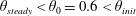
The first initial condition that we select is a partial concentric annulus that is in contact with the inner boundary of the annulus. For our choice of
 ${\mathcal{V}}$
we arrive at
${\mathcal{V}}$
we arrive at
 $\unicode[STIX]{x1D703}_{init}\approx 0.617<\unicode[STIX]{x1D703}_{steady}$
.
$\unicode[STIX]{x1D703}_{init}\approx 0.617<\unicode[STIX]{x1D703}_{steady}$
.
A time series of the evolution of the interface is shown in figure 11. The dense fluid and light fluid begin to exchange; however, owing to the curvature of the domain, the current is restricted and comes to rest with a horizontal interface on each side of the annulus, with a conjoining section of fluid in contact with the inner boundary.
A comparison could be drawn between the early-time classical exchange flow, before pinch-off, analogously to that shown in § 4.1.

Figure 11. Results for
 $\unicode[STIX]{x1D703}_{init}\approx 0.617$
. Each panel corresponds to different parts of the flow evolution at various times
$\unicode[STIX]{x1D703}_{init}\approx 0.617$
. Each panel corresponds to different parts of the flow evolution at various times
 $t$
. (a) The initial state, (b) an exchange flow develops but is restricted by the curvature of the annulus and (c) steady state.
$t$
. (a) The initial state, (b) an exchange flow develops but is restricted by the curvature of the annulus and (c) steady state.
5.2 Deepening and squeezing
To analyse the case of the draining film flow,
 $\unicode[STIX]{x1D703}_{init}>\unicode[STIX]{x1D703}_{steady}$
, we keep the parameters the same as in § 5.1. However, now we select an initial partial concentric annulus
$\unicode[STIX]{x1D703}_{init}>\unicode[STIX]{x1D703}_{steady}$
, we keep the parameters the same as in § 5.1. However, now we select an initial partial concentric annulus
 $h_{0}=0.4$
, which requires
$h_{0}=0.4$
, which requires
 $\unicode[STIX]{x1D703}_{init}\approx 1.021$
. A visualisation of the time evolution of the interface in this case can be seen in figure 12. The dense fluid at each of the far ends of the annulus develops a travelling front moving azimuthally, due to the advection, but also flattening, due to the diffusion. Movement of dense fluid downslope causes a deepening of the fluid in the region
$\unicode[STIX]{x1D703}_{init}\approx 1.021$
. A visualisation of the time evolution of the interface in this case can be seen in figure 12. The dense fluid at each of the far ends of the annulus develops a travelling front moving azimuthally, due to the advection, but also flattening, due to the diffusion. Movement of dense fluid downslope causes a deepening of the fluid in the region
 $-\unicode[STIX]{x1D703}_{steady}<\unicode[STIX]{x1D703}<\unicode[STIX]{x1D703}_{steady}$
. This deepening of the pool of dense fluid at the base of the annulus leads to formation of a film of light fluid, which is gradually squeezed out from the region between the inner boundary and deepening layer of dense fluid. Eventually the system asymptotes to its final piecewise steady state.
$-\unicode[STIX]{x1D703}_{steady}<\unicode[STIX]{x1D703}<\unicode[STIX]{x1D703}_{steady}$
. This deepening of the pool of dense fluid at the base of the annulus leads to formation of a film of light fluid, which is gradually squeezed out from the region between the inner boundary and deepening layer of dense fluid. Eventually the system asymptotes to its final piecewise steady state.

Figure 12. Results for
 $\unicode[STIX]{x1D703}_{init}\approx 1.02$
. Each panel corresponds to different parts of the flow evolution at various times
$\unicode[STIX]{x1D703}_{init}\approx 1.02$
. Each panel corresponds to different parts of the flow evolution at various times
 $t$
. (a) The initial state, (b) the fluid flows down the outer wall with a shock forming, (c) a thin film of light fluid forms between
$t$
. (a) The initial state, (b) the fluid flows down the outer wall with a shock forming, (c) a thin film of light fluid forms between
 $\pm \unicode[STIX]{x1D703}_{steady}$
, which is then squeezed out by the dense fluid
$\pm \unicode[STIX]{x1D703}_{steady}$
, which is then squeezed out by the dense fluid
 $\unicode[STIX]{x1D70C}_{O}$
, and (d) steady state.
$\unicode[STIX]{x1D70C}_{O}$
, and (d) steady state.
5.2.1 Squeeze film asymptotics
We can analyse the squeezing of the thin film by making an asymptotic approximation to (2.10). Firstly, we take the limit of non-dimensional gap width
 $\unicode[STIX]{x1D700}\rightarrow 0$
. Furthermore, since
$\unicode[STIX]{x1D700}\rightarrow 0$
. Furthermore, since
 $h\rightarrow 0$
, we can approximate the contribution of the
$h\rightarrow 0$
, we can approximate the contribution of the
 $(1-h)^{3}$
term as being 1. This leads to the simplified equation
$(1-h)^{3}$
term as being 1. This leads to the simplified equation
 $$\begin{eqnarray}\displaystyle \frac{\unicode[STIX]{x2202}h}{\unicode[STIX]{x2202}t}+3h^{2}\sin \unicode[STIX]{x1D703}\frac{\unicode[STIX]{x2202}h}{\unicode[STIX]{x2202}\unicode[STIX]{x1D703}}=-h^{3}\cos \unicode[STIX]{x1D703}. & & \displaystyle\end{eqnarray}$$
We can solve this using the method of characteristics with
 $h(0)=h_{0}$
and
$h(0)=h_{0}$
and
 $\unicode[STIX]{x1D703}(0)=\unicode[STIX]{x1D703}_{0}$
,
$\unicode[STIX]{x1D703}(0)=\unicode[STIX]{x1D703}_{0}$
,
 $$\begin{eqnarray}\displaystyle & \displaystyle \frac{\text{d}h}{\text{d}s}=-h\quad \Rightarrow \quad h=h_{0}\text{e}^{-s}, & \displaystyle\end{eqnarray}$$
 $$\begin{eqnarray}\displaystyle & \displaystyle \frac{\text{d}\unicode[STIX]{x1D703}}{\text{d}s}=3\tan \unicode[STIX]{x1D703}\quad \Rightarrow \quad \unicode[STIX]{x1D703}=\arcsin (\text{e}^{3s}\sin \unicode[STIX]{x1D703}_{0}), & \displaystyle\end{eqnarray}$$
 $$\begin{eqnarray}\displaystyle & \displaystyle \frac{\text{d}t}{\text{d}s}=\frac{1}{h^{2}\cos \unicode[STIX]{x1D703}}=\frac{1}{h_{0}^{2}\text{e}^{-2s}\sqrt{1-\text{e}^{6s}\sin ^{2}\unicode[STIX]{x1D703}_{0}}}. & \displaystyle\end{eqnarray}$$
Again we can find solutions
 $h(\unicode[STIX]{x1D703},t)$
in terms of the time-like parameter
$h(\unicode[STIX]{x1D703},t)$
in terms of the time-like parameter
 $s$
given implicitly in terms of
$s$
given implicitly in terms of
 $t$
by the relation
$t$
by the relation
 $$\begin{eqnarray}t=f(\unicode[STIX]{x1D703}_{0})+\frac{\text{e}^{2s}\,\text{}_{2}F_{1}({\textstyle \frac{1}{3}},{\textstyle \frac{1}{2}};{\textstyle \frac{4}{3}};\text{e}^{6s}\sin ^{2}\unicode[STIX]{x1D703}_{0})}{2h_{0}^{2}},\end{eqnarray}$$
where
 $\text{}_{2}F_{1}$
is the Gaussian hypergeometric function. Eliminating
$\text{}_{2}F_{1}$
is the Gaussian hypergeometric function. Eliminating
 $s$
gives us the general solution to (5.1)
$s$
gives us the general solution to (5.1)
 $$\begin{eqnarray}\displaystyle f\left(\arcsin \left(\frac{h^{3}\sin \unicode[STIX]{x1D703}}{h_{0}^{3}}\right)\right)=t-\frac{\text{}_{2}F_{1}\left({\textstyle \frac{1}{3}},{\textstyle \frac{1}{2}};{\textstyle \frac{4}{3}};\sin ^{2}\unicode[STIX]{x1D703}\right)}{2h^{2}}. & & \displaystyle\end{eqnarray}$$
We can use the same initial condition
 $h_{0}=0.4$
as in the full numerical simulation of § 5.2 and an angle
$h_{0}=0.4$
as in the full numerical simulation of § 5.2 and an angle
 $\unicode[STIX]{x1D703}_{0}=0$
at the centre of the film to check our asymptotic approximation. That particular choice of
$\unicode[STIX]{x1D703}_{0}=0$
at the centre of the film to check our asymptotic approximation. That particular choice of
 $\unicode[STIX]{x1D703}_{0}$
leads to an analytical expression for the depth of the fluid as a function of time:
$\unicode[STIX]{x1D703}_{0}$
leads to an analytical expression for the depth of the fluid as a function of time:
 $$\begin{eqnarray}h=\frac{h_{0}}{\sqrt{1+2h_{0}^{2}t}}.\end{eqnarray}$$
As can be seen in figure 9(b) the numerical solution is in good agreement with this approximate solution. This asymptotic solution suggests that the system takes an infinite amount of time to adjust to equilibrium.
5.3 Time adjustment
As before in § 4.4 we can take a sweep of the
 $\unicode[STIX]{x1D703}_{init}$
space for a given volume of fluid and calculate the time taken for the difference in area to adjust to within 5 %, 10 % and 20 % of the final steady state. Figure 10(b) shows how the adjustment time
$\unicode[STIX]{x1D703}_{init}$
space for a given volume of fluid and calculate the time taken for the difference in area to adjust to within 5 %, 10 % and 20 % of the final steady state. Figure 10(b) shows how the adjustment time
 $t_{adjust}$
varies with the initial angle
$t_{adjust}$
varies with the initial angle
 $\unicode[STIX]{x1D703}_{init}$
. The large-volume regime is qualitatively different from the small-volume regime. The two values of dimensionless adjustment time
$\unicode[STIX]{x1D703}_{init}$
. The large-volume regime is qualitatively different from the small-volume regime. The two values of dimensionless adjustment time
 $t_{adjust}(5\,\%)$
for the two simulations in §§ 5.1 and 5.2 are
$t_{adjust}(5\,\%)$
for the two simulations in §§ 5.1 and 5.2 are
 $t_{adjust}=0.6$
and 126.4, respectively. For small values of
$t_{adjust}=0.6$
and 126.4, respectively. For small values of
 $\unicode[STIX]{x1D703}_{init}$
the difference between the initial area and the steady-state area is small, so the adjustment time is relatively fast. As
$\unicode[STIX]{x1D703}_{init}$
the difference between the initial area and the steady-state area is small, so the adjustment time is relatively fast. As
 $\unicode[STIX]{x1D703}_{init}$
increases, the difference in volumes increases, so the adjustment time increases.
$\unicode[STIX]{x1D703}_{init}$
increases, the difference in volumes increases, so the adjustment time increases.
6 Discussion and summary
We have demonstrated how two fluids confined within an annulus and with different density can adjust to equilibrium from an initial symmetric distribution. The adjustment time to steady state can vary considerably based on the initial mass and distribution of the two fluids within the annulus. As discussed previously, the distribution of cement inside a wellbore is crucial to the stability and integrity of the well and ultimately has important implications for any directional drilling project. The setting time of cement used for the mud displacement process is
 ${\sim}O(10^{3})$
s (Siddiqi Reference Siddiqi2012). If we introduce some typical values for the time scaling used in (2.8b
), i.e.
${\sim}O(10^{3})$
s (Siddiqi Reference Siddiqi2012). If we introduce some typical values for the time scaling used in (2.8b
), i.e.
 $R=0.1$
m,
$R=0.1$
m,
 $H=0.01$
m,
$H=0.01$
m,
 $\unicode[STIX]{x0394}\unicode[STIX]{x1D70C}=10~\text{kg}~\text{m}^{-3}$
and
$\unicode[STIX]{x0394}\unicode[STIX]{x1D70C}=10~\text{kg}~\text{m}^{-3}$
and
 $\unicode[STIX]{x1D707}=1~\text{kg}~\text{m}^{-1}~\text{s}^{-1}$
, we find a relationship
$\unicode[STIX]{x1D707}=1~\text{kg}~\text{m}^{-1}~\text{s}^{-1}$
, we find a relationship
 $t\approx 30\hat{t}$
. Looking at the non-dimensional adjustment time to 5 % in §§ 4.1–4.3, 5.1 and 5.2, we can see this corresponds to dimensional time adjustments of approximately 510 s, 414 s, 1533 s, 18 s and 3792 s, respectively. So we can see that the setting time of cement is comparable to the adjustment time of the flow. This demonstrates that the initial distribution of dense fluid is important, as it could have an undesirable distribution around the annulus as it begins to set, perhaps allowing for non-cemented and therefore highly permeable channels around the casing to develop.
$t\approx 30\hat{t}$
. Looking at the non-dimensional adjustment time to 5 % in §§ 4.1–4.3, 5.1 and 5.2, we can see this corresponds to dimensional time adjustments of approximately 510 s, 414 s, 1533 s, 18 s and 3792 s, respectively. So we can see that the setting time of cement is comparable to the adjustment time of the flow. This demonstrates that the initial distribution of dense fluid is important, as it could have an undesirable distribution around the annulus as it begins to set, perhaps allowing for non-cemented and therefore highly permeable channels around the casing to develop.


