2.1. Property models

In order to define the thermodynamic and transport properties of the fluid forming the heated jet, a distinction between primary and secondary flow quantities is introduced. The former represents the minimum set of quantities used to describe the flow, while the term property model is used to define the ensemble of relations used to obtain the secondary quantities from primary thermodynamic quantities. The lists of primary/secondary quantities depend on the thermodynamic and chemical assumptions of the flow, and are summarized in table 1.

Table 1. List of the primary/secondary variables chosen to describe the flow. The $H_{{m}}$, $F$ and $G$ quantities are grouping terms introduced by Malik & Anderson (Reference Malik and Anderson1991) for high-enthalpy flows, while $\zeta$ is the compressibility factor from (2.7).

The relations between primary and secondary quantities are expected to influence the stability features of the flow through two means: (i) indirectly, by influencing the distribution of primary quantities through transport phenomena in the governing equations; (ii) directly through secondary quantities’ base state values and perturbation's expansion in the stability equations (see Appendix A.1).

Similarly to a previous study (Demange & Pinna Reference Demange and Pinna2020), two main thermodynamic and chemical assumptions are considered in order to model the flow. The first considers air to be a single CPG with no chemical activity, as in most of the literature on heated jet instabilities (Lesshafft & Huerre Reference Lesshafft and Huerre2007; Balestra et al. Reference Balestra, Gloor and Kleiser2015; Chakravarthy et al. Reference Chakravarthy, Lesshafft and Huerre2018). The second stems from high-enthalpy flow literature (Anderson Reference Anderson2006) and uses a mixture of calorically perfect species allowing for dissociation reactions and vibrational excitation. Both assumptions are detailed below.

2.1.1. Single species CPG

By definition, the CPG assumption relies on a constant isobaric specific heat $c_p=1004$, 5 J kg$^{-1}$ K$^{-1}$ (for air), linearly relating the temperature to the static enthalpy: $h=c_pT$. Furthermore, the Prandtl number is imposed to be constant, and set to a common value for diatomic gases $Pr=0.7$. As a single air species is considered, the density is expressed through the state equation

(2.4)\begin{equation} \rho = p T \gamma M^2. \end{equation}

While performing simulations and stability analyses, the influence of transport phenomena on the hydrodynamic features of the jets is investigated by considering the following two formulations of the viscosity and thermal conductivity.

1. (i) The CPG-CP model assumes constant transport properties: $\mu =cst$ and $\kappa =cst$, which is commonly found in stability analyses of low-density jets (Lesshafft & Huerre Reference Lesshafft and Huerre2007; Balestra Reference Balestra2013; Chakravarthy et al. Reference Chakravarthy, Lesshafft and Huerre2018) but is a rough approximation in the viscous regime (Demange & Pinna Reference Demange and Pinna2020).

2. (ii) The CPG-VP model assumes temperature-dependent transport properties. The viscosity is obtained from Sutherland's law (Sutherland Reference Sutherland1893)

   (2.5)\begin{equation} \mu = \mu_{{ref}} +\left(\frac{T}{T_{{ref}}}\right)^{{3}/{2}} \frac{T_{{ref}} + S_{{su}}}{T + S_{{su}}}, \end{equation}
   where $\mu _{{ref}}=1789\times 10^{-5}$ kg m$^{-1}$ s$^{-1}$, $T_{{ref}}=288$ K and $S_{{su}}=110$ K. While the thermal conductivity is obtained from $\kappa =\mu c_pPr^{-1}$.

2.1.2. Equilibrium mixture of gases (LTE)

When increasing the temperature of a gas (at constant pressure), the CPG assumption fails due to the excitation of different energy modes (rotational, vibrational and electronic) and the rise of chemical processes (Anderson Reference Anderson2006). Therefore, a more accurate model considers the air as a mixture ‘$\mathcal {S}$’ of calorically perfect species ‘$s$’, with a fixed elemental composition and volume percentages of 21 % ${\rm O}_2$ and 79 % ${\rm N}_2$. The composition of the gas and chemical reactions accounted for correspond to the ‘air-11’ mixture from Park (Reference Park1993). The same mixture was used in a previous study (Demange et al. Reference Demange, Chazot and Pinna2020), and the corresponding concentrations $Y_s=\rho _s/\rho$ are plotted in figure 1. Thus, the density of the mixture is defined as

(2.6)\begin{equation} \rho = \sum_{s\in\mathcal{S}} \rho_{{s}}. \end{equation}

Figure 1. Concentration of the 11-species composing the air mixture from Park (Reference Park1993) with respect to the temperature ratio $S=T_{\infty }/T_{{c}}$, assuming $T_{\infty }=350$ K and pressure $p_{{s}}=100$ mbar: (a) shows the neutral species; (b) shows the charged species.

Furthermore, we assume that the characteristic times needed for the chemical reactions and energy modes to reach an equilibrium state are negligible compared with the flow's characteristic time $\tau _{{flow}}$. Consequently, the mixture is said to be in local thermodynamic and chemical equilibrium, abbreviated here to ‘LTE’. This implies that, for a given temperature and pressure, the mixture composition $Y_s(T,p)$ is fully determined, and that a single temperature is needed to describe the flow. The governing equations are then completed by the mixture state equation given as

(2.7)\begin{equation} H_{{m}} p = \rho T \zeta, \end{equation}

where $\zeta =\mathscr {M}_{{undiss}}/\mathscr {M}$ is the compressibility factor obtained from the mixture's molar mass $\mathscr {M}$ and $\mathscr {M}_{{undiss}}=0,21\mathscr {M}_{O_2}+0,79\mathscr {M}_{N_2}$, and $H_{{m}}=u_{{c}}^2/(T_{{c}}\mathcal {R})$ is a grouping term introduced by Malik & Anderson (Reference Malik and Anderson1991). This form of the state equation implies that $T_{\infty }/T_{{c}}\neq \rho _{{c}}/\rho _{\infty }$ at constant pressure, unlike with the CPG assumption.

Species thermodynamic properties are obtained similarly to Miró Miró et al. (Reference Miró Miró, Beyak, Pinna and Reed2019), assuming them to behave as a rigid rotor and harmonic oscillator. The mixture's enthalpy is then obtained from

(2.8)\begin{equation} h = \sum_{s\in \mathcal{S}} Y_sh_s. \end{equation}

The resulting nonlinear relation between the static enthalpy and the temperature is illustrated in figure 2. Transport properties $\mu (T,p)$ and $\kappa (T,p)$ are computed from approximations of the Chapman and Enskog gas theory, while barodiffusion and elemental demixing are ignored (Miró Miró et al. Reference Miró Miró, Beyak, Pinna and Reed2019).

Figure 2. (a) Nonlinear relation between the mixture's static enthalpy and the temperature in LTE with $p_{{s}}=100$ mbar; resulting LTE inlet formulations imposing either a top-hat profile of temperature (LTE-T ——) or static enthalpy (LTE-h - - -) for $S=0.0667$.

2.2. Unsteady simulations and steady states

Simulations of the heated jets are performed to obtain both the steady state solutions $\bar {q}=[\bar {\boldsymbol {u}},\bar {T},\bar {p}]$ used in the stability analysis, and the unsteady evolution of the flow $q(\boldsymbol {x},t)$. To this end, an existing DNS code (Nichols Reference Nichols2005; Chandler et al. Reference Chandler, Juniper, Nichols and Schmid2012; Qadri et al. Reference Qadri, Chandler and Juniper2015, Reference Qadri, Chandler and Juniper2018) is used, which solves the low Mach number approximation of the axisymmetric Navier–Stokes equations. This formulation effectively splits the pressure into a slow thermodynamic component $p^{(0)}$, assumed constant, and a fast hydrodynamic component $p^{(1)}$, which is the solution to a Poisson equation. The resulting equations allow for density variations due to temperature gradients, while neglecting those associated with the pressure.

The ‘top-hat’ distributions of temperature and velocity (number $2$ from Michalke Reference Michalke1984) are imposed at the domain's inlet ($z=0$), while varying the temperature ratio in the range $S\in [0.0667;0.4]$. Values of $S$ and other inlet parameters studied are given in table 2. The choice of Reynolds’ number is based on typical values found at the inlet of the VKI Plasmatron plasma jet (Demange et al. Reference Demange, Chazot and Pinna2020), while the shear-layer thickness is given a middle value from ranges studied in the literature (Lesshafft & Huerre Reference Lesshafft and Huerre2007). A co-flow of $1\,\%$ of the centreline velocity is also injected to improve numerical stability. Remaining boundary conditions mimic a semi-infinite domain allowing for gas entrainment on the lateral sides of the domain (Nichols, Schmid & Riley Reference Nichols, Schmid and Riley2007; Chandler et al. Reference Chandler, Juniper, Nichols and Schmid2012). The domain studied extends to respectively $[0;30]$ and $[-5;5]$ diameters $(D=2R)$ in the streamwise and radial directions. In unsteady simulations a non-dimensional time step of ${\rm \Delta} t = 0.005$ is imposed after initializing the flow by copying the inlet profiles through the domain. Unlike the analysis of Lesshafft, Huerre & Sagaut (Reference Lesshafft, Huerre and Sagaut2007), no perturbation is injected in the flow because the initialization procedure was found to be enough to trigger self-sustained oscillations.

Table 2. Inlet parameters chosen for the simulations of synthetic heated jet flows in this study, $\theta$ indicates the shear-layer momentum thickness. In the case of the CPG-CP flow, an additional simulation is performed at $S = 0.0909$.

Steady solutions are obtained using a selective frequency damping method introduced by Åkervik et al. (Reference Åkervik, Brandt, Henningson, Hæpffner, Marxen and Schlatter2006) and implemented by Chandler et al. (Reference Chandler, Juniper, Nichols and Schmid2012) in the DNS. Simulations are considered as converged once residuals reach $10^{-6}$, and examples of steady states are plotted in figure 3. Both steady/unsteady simulations use the same mesh with $(713;513)$ grid points along the $(\boldsymbol {e}_z;\boldsymbol {e}_r)$ directions.

Figure 3. Examples of the heated jets steady streamwise velocity (a) and temperature (b) for $S=0.0667$, $Re_D=400$ and $R/\theta =20$ with the CPG-VP and LTE-T flow models.

The different flow models presented in § 2.1 are implemented in the DNS code, which originally considered only CPG flows with constant transport properties. Modifications of the DNS code for the CPG-VP model are straightforward, while details of the LTE implementation are given below.

2.2.1. High-enthalpy jet simulations

When considering the flow as an equilibrium mixture, the low Mach number framework is replaced by a low Eckert number expansion of the Navier–Stokes equations, which leads to a similar system of non-dimensional equations

(2.9a)$$\begin{gather} \frac{\partial \rho^{(0)}}{\partial t} + \boldsymbol{\nabla}(\rho u)^{(0)} = 0, \end{gather}$$

(2.9b)$$\begin{gather}\frac{\partial(\rho u)}{\partial t} + \boldsymbol{\nabla} (\rho u u) = \boldsymbol{\nabla} p^{(1)} -\frac{S_{\rho}}{Re_D}\boldsymbol{\nabla}(\tau), \end{gather}$$

(2.9c)$$\begin{gather}\rho\frac{{\rm D} h}{{\rm D} t} = \frac{S_{\rho}}{Re_D Pr_2}\boldsymbol{\nabla}(\lambda \boldsymbol{\nabla} T), \end{gather}$$

where the reference quantities are chosen at the inlet centreline, with the exception of the reference density $\rho _{\infty }$ which is taken in the outer flow and the reference static enthalpy $h_{{ref}}=p_{\infty }/\rho _{\infty }(=h_{\infty } - e_{\infty })$, where $e_{\infty }$ is the internal energy in the outer flow. The resulting non-dimensional numbers are defined as

(2.10a–d)\begin{equation} S_{\rho} = \frac{\rho_{{c}}}{\rho_{\infty}},\quad Re_D = \frac{\rho_{{c}} u_{{c}} D}{\mu_{{c}}},\quad Ec_2 = \frac{\rho_{\infty} u_{{c}}^2}{p_{\infty}}\quad \text{and}\quad Pr_2 = \frac{\mu_{{c}}}{\kappa_{{c}}T_{{c}}}\frac{p_{\infty}}{\rho_{\infty}}. \end{equation}

As flow properties depend on the pressure $p$ in LTE, a low static pressure of $p_{{s}}=100$ mbar is prescribed, which is representative of plasma wind tunnel conditions where the LTE assumption was validated experimentally (Cipullo Reference Cipullo2010). Although the value of $p_{{s}}$ is fairly low, the continuum flow assumption is still valid because the Knudsen number of the flow remained below $0.01$ for all cases.

Based on the nonlinear relation relating the static enthalpy to temperature in LTE (see figure 2a), two formulations of the inlet energy condition are compared against each other in this study (see figure 2b).

1. (i) The LTE-h model imposes a top-hat profile of static enthalpy at the inlet. For each value of $S$, an equivalent enthalpy ratio $h_{\infty }/h_{{c}}$ is obtained and an equivalent temperature inlet profile is retrieved by inverting the enthalpy-temperature relation.

2. (ii) The LTE-T model imposes a top-hat profile of temperature at the inlet, similarly to the energy condition of the CPG models.

We emphasize that both conditions are not equivalent for the same value of $S$, because the LTE-h inlet condition yields a temperature layer slightly shifted outward of the shear layer, with humps due to dissociation relations (Demange & Pinna Reference Demange and Pinna2020). The LTE-h model also introduces slightly more thermal energy in the flow than the LTE-T one. Details of the numerical implementation of the LTE model are given in Demange, Qadri & Pinna (Reference Demange, Qadri and Pinna2019). Finally, we also stress that based on the current definition of the Reynolds number, the mass flow injected into the simulations is modified by the CPG or LTE assumption imposed on the flow. In practice, the LTE assumption results in an increased inlet mass flow with respect to its CPG counterpart, in particular at low $S$.

2.3. Linear stability analyses

The analysis of the jets’ stability features is carried out within the classical linear framework, decomposing flow quantities into the sum of a base state value and small non-interacting axisymmetric perturbations: $q(\boldsymbol {x},t) =\bar {q}(\boldsymbol {x}) + \varepsilon q'(\boldsymbol {x},t)$ with $\varepsilon \ll 1$. Perturbations take the shape of normal modes of the flow by performing a Fourier transform in the homogeneous spatial directions of the flow and a Laplace transform in time

(2.11)\begin{equation} q'(\boldsymbol{x},t) =\tilde{q}(\boldsymbol{x})\,{\rm e}^{{\rm i}\phi} +c.c., \end{equation}

where $\tilde {q}$ is the complex shape function, $\phi$ is the complex phase function and ‘$c.c.$’ denotes the complex conjugate needed for $q'$ to be a real quantity.

In the following, both the local and BiGlobal approaches are considered. Within the local formulation, one must ensure a separation of scales between the development length of the flow $\mathcal {L}_{{flow}}$ and typical perturbation wavelengths (section 3 in Huerre & Monkewitz Reference Huerre and Monkewitz1990), allowing perturbations to take a wave-like form in the $\boldsymbol {e}_z$ and $\boldsymbol {e}_{\theta }$ directions, with a phase function given by (2.12a). For the BiGlobal analysis, the flow is considered homogeneous only along the azimuthal direction, leading to the so-called global modes (Theofilis Reference Theofilis2003) with a phase function given by (2.12b). In the phase functions

(2.12a)$$\begin{gather} {\phi = \alpha z - \omega t}, \end{gather}$$

(2.12b)$$\begin{gather}{\phi ={-} \omega t}, \end{gather}$$

$\alpha$ denotes the streamwise wavenumber and $\omega$ the complex angular frequency.

Once completed with the boundary conditions of Appendix A.2, the stability equations are obtained by introducing the linear ansatz and modal perturbations into the compressible Navier–Stokes equations (2.1). Finally, the generalized eigenvalue problem of the form

(2.13)\begin{equation} (\underline{\underline{A}} + \underline{\underline{B}}\omega)\tilde{q}=0 \end{equation}

is retrieved, where $\underline {\underline {B}}$ is the matrix containing terms multiplying $\omega$, $\underline {\underline {A}}$ contains the remaining terms including $\alpha$ and $\tilde {q}$ is the eigenvector array associated with the eigenvalue $\omega$. Matrices $\underline {\underline {A}}$ and $\underline {\underline {B}}$ are detailed in a previous study (Demange & Pinna Reference Demange and Pinna2020) for the local problem, and in the supplementary materials of this paper for the BiGlobal problem available at https://doi.org/10.1017/jfm.2022.43. The resulting eigenvalue problems are solved in the VESTA toolkit (Pinna Reference Pinna2013), using a Chebyshev collocation method for the local problem, and the sixth-order finite difference method from the UEFD Fortran library by Hermanns & Hernández (Reference Hermanns and Hernández2008) for the heavier BiGlobal problem.

In order to determine the noise amplifier (globally stable) or self-excited oscillator (globally unstable) nature of the flows (Huerre Reference Huerre2000), the spatio-temporal formulation of the local analysis is used, allowing one-dimensional waves to grow both in space $(\alpha \in \mathbb {C})$ and time $(\omega \in \mathbb {C})$. Following Huerre & Monkewitz (Reference Huerre and Monkewitz1985), absolute instabilities are found at each streamwise position by examining the sign of the absolute growth-rate ${\rm Im}(\omega ^*)$, obtained where iso-contours of $\omega$ form a valid (Briggs Reference Briggs1964; Bers Reference Bers1984) saddle point in the complex wavenumber plane $(\partial _{\alpha \in \mathbb {C}}\omega ^*=0)$. As summarized by Coenen & Sevilla (Reference Coenen and Sevilla2012), the actual transition to a globally unstable flow depends on the position and extent of the resulting absolute region defined by $\sigma (z)\geq 0$ (Chomaz, Huerre & Redekopp Reference Chomaz, Huerre and Redekopp1988; Couairon & Chomaz Reference Couairon and Chomaz1999). Using the BiGlobal approach, the stable/unstable nature of the global (linear) mode is directly given by the growth-rate ${\rm Im}(\omega )$ in the phase function of (2.12b).

3.1. Onset of self-sustained oscillations

According to the convective to absolute boundary diagram displayed in figure 4(a) from Demange & Pinna (Reference Demange and Pinna2020), all the inlet conditions defined in table 2 are already absolutely unstable. As detailed in § 4.1, this does not necessarily mean that all conditions studied are globally unstable in the sense of Chomaz (Reference Chomaz2005). However, the resulting jets are expected to be close to the Hopf bifurcation (Chakravarthy et al. Reference Chakravarthy, Lesshafft and Huerre2018), and to experience self-sustained oscillations once the temperature ratio is lowered below a threshold value, $S_{{H}}$ (Monkewitz & Sohn Reference Monkewitz and Sohn1998; Qadri et al. Reference Qadri, Chandler and Juniper2015; Coenen et al. Reference Coenen, Lesshafft, Garnaud and Secilla2017). A summary of the resulting stable and unstable configurations is given in figure 4(b), which shows a strong dependence of the bifurcation and the onset of the periodic regime to the TTP model used to describe the flow.

Figure 4. (a) Comparison of the inlet conditions chosen for the simulations of the synthetic heated jet (- - -) against the convective-to-absolute instability boundary obtained in a previous study (Demange & Pinna Reference Demange and Pinna2020) with the CPG-CP ($\triangle$), CPG-VP ($\circ$) and LTE-h ($\diamond$) models for the one-dimensional inlet profiles (the greyed area denotes an absolutely unstable parallel flow). (b) Diagram representing the outcome of unsteady simulations, cases either exhibit self-sustained oscillations (filled symbols) or converge towards a steady state (open symbols).

For non-reacting flows (CPG), different models of the transport properties ($\mu$ and $\kappa$) have a strong influence on the global stability behaviour. When uniform and constant properties are prescribed (CPG-CP), the jets remain globally stable for most of the conditions studied and the bifurcation is only observed for temperature ratios below $S<0.1$. This is confirmed by an additional simulation performed with this model for $S = 0.0909$, where the flow is globally unstable. An example of the CPG-CP simulation is provided in the supplementary materials (see movie_1). However, if the temperature-dependent transport properties are taken into account (CPG-VP), the jets undergo a bifurcation to a globally unstable regime as soon as $S\leq 0.2225$.

In the case of chemically reacting flows (LTE), the bifurcation is observed for slightly lower temperature ratios $(S_{\text {H}}=0.5)$ for both types of energy inlet. Given that, for this temperature ratio, Sutherland's law remains accurate and that dissociation reactions are yet to be activated, the bifurcation delay between the LTE and CPG-VP jets is probably related to the vibrational excitation ($\approx$900 K Anderson Reference Anderson2006), which marks the end of the CPG assumption's validity. Interestingly, a restabilization is observed for the LTE jets with top-hat inlet profiles of static enthalpy (LTE-h) as $S<0.125$. As this restabilization is not observed with the LTE-T jets, these results confirm the importance of the inlet profiles’ shape on the stability features (Coenen & Sevilla Reference Coenen and Sevilla2012).

In a recent study, Zhu, Gupta & Li (Reference Zhu, Gupta and Li2017) proposed a criterion to predict the parameters of Hopf bifurcations in low-density jets, based on experimental and numerical results. It is worth mentioning that most of the low-density jets studied by Zhu et al. (Reference Zhu, Gupta and Li2017) are in fact light jets, where the density gradient is created by injecting a lighter species (such as helium) into a quiescent heavier gas. However, heated jets are known to present different profiles to those of light jets (Coenen & Sevilla Reference Coenen and Sevilla2012), thus altering the stability properties. Using the formula from Zhu et al. (Reference Zhu, Gupta and Li2017), bifurcation parameters can be related through

(3.1)\begin{equation} S^{{-}1}_{\rho,{H}} = \frac{(Re_{{D}}^{{-}1} - a)}{bD\theta_0^{{-}1}} + 1, \end{equation}

where $a=-3.785\times 10^{-4}$ and $b=1.019\times 10^{-5}$. Using the same definition of $\theta _0$ as Zhu et al. (Reference Zhu, Gupta and Li2017) and setting $Re_{{D}}=400$ in (3.1), this criterion predicts a value of $S_{\rho,{H}}=0.1338$, which is approximately half the value found in our simulations with the CPG-VP model.

3.2. Behaviour of the globally unstable flows

Among the globally unstable jets, three types of behaviour are observed depending on the TTP model and value of $S$ imposed. Evidence of these types of behaviour are provided by snapshots of the non-dimensional azimuthal vorticity ($\varOmega = \partial _z u - \partial _r w$), and space–time diagrams of radial velocity perturbations in the shear layer $v'=v(z,r\!=\!1,t)-\hat {v}(z,r\!=\!1)$, where $\hat {v}$ is the time-averaged radial velocity. Both are displayed in figure 5 for cases computed with the LTE-T model, because it is found to display all three behaviours depending on the value of $S$.

Figure 5. Illustration of the three different behaviours of the unsteady heated jets, here for the LTE-T model at $S=[0.2; 0.111; 0.0667]$ (top to bottom): shown through (a) snapshots of the (non-dimensional) vorticity $\varOmega = \partial _z u - \partial _r w$; and through (b) spatio-temporal diagrams of the radial velocity perturbations $v'=v(z,r=1, t)-\hat {v}(z,r=1)$, where $\hat {v}$ is the time-averaged value. Animations of the corresponding vorticity contours are available in the supplementary materials (movie_2a, movie_2b and movie_2c).

In globally unstable jets with moderate temperature ratios $(S\geq 0.125)$, vortices are produced periodically in the shear layer before moving downstream without interacting with each other (see movie2a in supplementary materials). Vortical structures growing near the inlet are then advected downstream while diffusing. A slight movement of their centres towards the jet's centreline is also observed during this process.

When increasing the centreline temperature, periodic vortex coupling events occur after the transient regime for the LTE-T model at $S=[0.1;0.111]$ (see movie2b in supplementary materials) and the CPG-VP model at $S=0.0667$. These events consistently remain at a fixed streamwise position, $z_{pair}\approx 10D$ for both LTE cases and $z_{pair}\approx 8D$ for the CPG-VP case. Similar phenomena were also described in simulations by Lesshafft et al. (Reference Lesshafft, Huerre and Sagaut2007) for all their unstable cases with $R/\theta >10$ and $Re_D=7500$, and in experiments by Kyle & Sreenivasan (Reference Kyle and Sreenivasan1993) in light jets with thin shear layers and Reynolds number above $Re_D>2000$. The present observations suggest that the occurrence of these events depends more strongly on the temperature ratio and precise shape of the profiles (imposed by changes of the TTP models) in a highly viscous regime.

Finally, increasing the centreline temperature to even lower temperature ratios $(S=0.0667)$ is found to produce a third type of behaviour only in the case of the LTE-T jets. Vortices are then produced in pairs, and closely follow each other without coupling before the diffusion of these structures renders any observation impracticable (see movie2c in supplementary materials). Although the initial phase is physically accurate, this is not the case during the later phase because these unstable structures would break down more quickly in three-dimensional simulations.

3.3. Frequency content

Unsteady simulations are also used to extract the frequency of self-sustained oscillations observed in the globally unstable cases. As seen in the time history of the radial velocity fluctuations displayed in figure 6, unstable cases present a remarkably periodic behaviour, in agreement with previous experimental (Monkewitz et al. Reference Monkewitz, Bechert, Barsikow and Lehmann1990; Hallberg & Strykowski Reference Hallberg and Strykowski2006) and numerical (Lesshafft et al. Reference Lesshafft, Huerre and Sagaut2007) observations. For this figure, the reference time scale is chosen as $t_{ref}=D/w_c$. The frequency of these oscillations is recovered by performing a fast Fourier transform (FFT) analysis in the shear layer, at $(z,r)=(5;0.5)\times D$, where perturbations are amplified. Examples of the power spectra obtained for unstable cases are also given in figure 6. In the absence of vortex coupling, the spectrum contains the main frequency $\omega _r$ and higher harmonics (black spectrum in figure 6). In the cases where vortex coupling is observed (blue spectrum in figure 6), a first sub-harmonic is present on the left of the main peak at $1/2\omega _r$, as well as for higher frequencies ($3/2\omega _r$, $2\omega _r$, $5/2\omega _r$ and so on), similarly to (Monkewitz et al. Reference Monkewitz, Bechert, Barsikow and Lehmann1990; Lesshafft et al. Reference Lesshafft, Huerre and Sagaut2007).

Figure 6. Time evolution of the radial velocity (a) at $(z,r)=(5;0.5)D$ for the CPG-CP ($\cdots$) flow at $S=0.1429$, the CPG-VP (black ——) flow at $S=0.1429$ and the CPG-VP (blue ——) flow with vortex coupling at $S=0.0667$; FFT spectra (b) of the CPG-VP flows at $S=0.1429$ (black ——) and $S=0.0667$ (blue ——), ignoring the transient regime.

The main frequencies of self-sustained oscillations are given by the maximum of power spectra obtained from the FFT analysis for each case and are reported in table 3 in non-dimensional form: ${\rm Re}(\omega )=2{\rm \pi} D f/ w_c$. As seen from these results, the frequency of self-sustained oscillations decreases when the centreline temperature of the jet is increased.

Table 3. Main non-dimensional frequencies obtained from the FFT analysis of unsteady simulations at $z=5D$ and $r=D/2$ for each globally unstable model, ‘—’ indicates a stable case without periodic regime and ‘$*$’ an absence of simulation.

In the following, frequencies from the present study are compared against the universal frequency scaling proposed by Hallberg & Strykowski (Reference Hallberg and Strykowski2006) for low-density jets. This criterion estimates the global frequency based on inlet parameters such as the initial momentum thickness $\theta _0=\int ^{r_{0.1}}_{0}w(r)[1-w]\,{\rm d} r$, with $r_{0,1}=r(w=0.1)$, and viscous scale obtained from the inlet centreline kinematic viscosity $\nu =\mu _{{c}}/\rho _{{c}}$, while assuming top-hat-like inlet shapes

(3.2)\begin{equation} f D^2 \nu^{{-}1} = a + b Re\left( \frac{D}{\theta_0} \right)^{1/2} (1+S_{\rho}^{1/2}), \end{equation}

with coefficients from Hallberg & Strykowski (Reference Hallberg and Strykowski2006), $a=-37$ and $b=0.034$. Similarly to the bifurcation criterion of Zhu et al. (Reference Zhu, Gupta and Li2017), the reference data of Hallberg & Strykowski (Reference Hallberg and Strykowski2006) includes mostly light jets results, except for the heated jets of Lesshafft et al. (Reference Lesshafft, Huerre, Sagaut and Terracol2005), and higher Reynolds numbers.

The comparison of the present simulations’ results with different TTP models against the frequency criterion is displayed in figure 7(a). Results show that the general trends from our DNS results are in good agreement with the proposed scaling, showing that this criterion can be used as a preliminary estimation for the global frequency of heated jets. However, curves from the different TTP models do not collapse onto each other, and display a shape similar to those obtained with the heated jet data of Lesshafft et al. (Reference Lesshafft, Huerre, Sagaut and Terracol2005) reported in Hallberg & Strykowski (Reference Hallberg and Strykowski2006, figure 8). This observation reinforces the argument that heated and light jets have different global stability behaviour, both in their bifurcation and frequency parameters.

Figure 7. Frequencies obtained from the unsteady DNS using the CPG-CP ($\triangle$), CPG-VP ($\circ$), LTE-h ($\diamond$) and LTE-T ($\triangledown$) TTP models; (a) shows the comparison between the present DNS results against the criterion as given by Hallberg & Strykowski (Reference Hallberg and Strykowski2006); (b) shows a similar criterion, this time with the compressible momentum thickness, resulting coefficients are given as $fD\nu ^{-1}=193.1 - 0.01608Re(D/\theta _0)^{1/2}(1+S^{1/2})$, and lead to a $R^2=0.93$ fitness. Note that for this figure only, $S$ is the density ratio.

Proposing a similar criterion for heated jets lies beyond the scope of the present study. Nonetheless, we note that this frequency scaling partly takes into account differences between the CPG and LTE models through changes of $\nu$ for the same values of $Re$ and $S$, but cannot account for modifications of the thermal layer such as those found when comparing the LTE-h and LTE-T formulations. Therefore, the same criterion is investigated for the variable property models using the compressible definition of the momentum thickness $\theta _0 = \int ^{r_{0.1}}_{0}w\rho [1-w]\,{\rm d} r$ in figure 7(b). The proposed fit displays a reversed orientation of the criterion, with new coefficients $a=193.1$ and $b=-0.01608$, but an improved linear fitness of $R^2=0.93$ with results from the LTE-h and LTE-T flow models collapsing to a common shape.

4.1. Prediction of the critical temperature ratios

First, typical results from the local and BiGlobal analyses are given for the $S=0.111$ case, where the centreline temperature is sufficiently high to bring out the differences between TTP models. Second, the analyses are generalized to the complete range of temperature ratios.

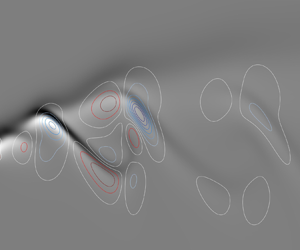
Figure 8(a) displays an example of the absolute growth rate along the $\boldsymbol {e}_z$ direction for the $S=0.111$ jet with each TTP model. Absolute regions start at the inlet and end where $\omega _i^*(z)=0$, which defines the absolute length $l_{ac}$. For configurations where the inlet profile is already absolutely unstable, previous nonlinear (Chomaz et al. Reference Chomaz, Huerre and Redekopp1988; Couairon & Chomaz Reference Couairon and Chomaz1999) and linear (Coenen & Sevilla Reference Coenen and Sevilla2012) analyses indicate that the occurrence of an unstable global mode depends on the streamwise extent of the absolute region. For the case plotted, the absolute lengths obtained with each TTP model are coherent with the DNS observations: the globally stable CPG-CP and LTE-h jets display shorter absolute regions than the globally unstable CPG-VP and LTE-T jets. Additionally, the perturbations at the inlet displayed in figure 8(b) are typical of the jet-column mode observed by Lesshafft & Huerre (Reference Lesshafft and Huerre2007) for this type of jet. An example of a BiGlobal analysis is then considered.

Figure 8. Results from the local linear analysis of the steady heated jets with $S=0.111$ and the CPG-CP ($\triangle$), CPG-VP ($\circ$), LTE-h ($\diamond$) and LTE-T ($\triangledown$) flow models: (a) absolute growth rate from the local analysis along the streamwise direction; (b) absolute value of the streamwise velocity (up) and pressure (down) perturbations corresponding to the absolute mode (——) at $z=5R$, BiGlobal mode perturbations (- - -) for the same case and position are added for comparison (CPG-VP only).

Figure 9(a) displays the BiGlobal spectra obtained with each TTP model for the same $S=0.111$ case. Similarly to previous BiGlobal analyses of low-density jets (Chakravarthy et al. Reference Chakravarthy, Lesshafft and Huerre2018; Qadri et al. Reference Qadri, Chandler and Juniper2018; Bharadwaj & Das Reference Bharadwaj and Das2019), the spectra include an isolated mode corresponding to the oscillations observed in simulations, and a continuous branch sensitive to the domain's length. In the present study no absorbing layer is added to the eigenvalue problem (EVP) (Lesshafft Reference Lesshafft2018), because the continuous branches remained stable. Similarly to the local analysis for the same $S$, BiGlobal results are coherent with the DNS observations: both the CPG-VP and LTE-T jets are linearly globally unstable, while the CPG-CP and LTE-h jets remain stable. This observation reveals both a strong influence of the inlet shapes and TTP modelling over the global stability features of viscous heated jets. The corresponding global mode shapes are given in figure 9(b) for each flow model. Perturbations of the stable global modes extend towards the end of the domain, while those of unstable modes have a more compact spatial structure for this case. For both the LTE-T and LTE-h jets, perturbations start closer to the inlet than for the CPG assumptions and are confined to a smaller radial extent. This is believed to be caused by the faster spreading of jets obtained with the LTE transport and thermodynamic properties. Global mode shapes are also compared against that of the local absolute mode with the CPG-VP model in figure 8(b), revealing that both methods yield similar features in the shear layer, but differ towards the centreline of the jet.

Figure 9. Results from the BiGlobal linear analysis of the heated jets with $S=0.111$: (a) spectra from the BiGlobal EVP with $m=0$ for the CPG-CP ($\triangle$), CPG-VP ($\circ$), LTE-h ($\diamond$) and LTE-T ($\triangledown$) flow models, isolated modes are indicated with filled symbols; (b) real part of BiGlobal isolated mode's temperature perturbations obtained with the different TTP models for the same case.

Results from the local and global analyses are then generalized to the complete range of temperature ratio $S$. Starting with the global analysis, the trend of the global growth rate as a function of $S$ are given in figure 10(a) for each of the TTP models. The growth rates obtained with each model are negative for the maximum value of $S$, and increase with decreasing $S$. In the case of the LTE-h jet, the growth rate remains negative for the whole range of $S$ and reaches a maximum for $S=0.1429$, and decreases for lower values of $S$. Despite the apparent mismatch with the simulations where the LTE-h jet does become globally unstable, the trends obtained are coherent with the restabilization observed. For the CPG-VP and LTE-T assumptions, the analysis over the steady state predicts a critical temperature ratio $S_{{H}}$ significantly lower than that observed in simulations. Similarly, the growth rate of the CPG-CP remains negative, although a bifurcation is observed around $S\approx 0.0909$ with this model. Consequently, all the viscous heated jets studied here are found to undergo a subcritical bifurcation, similarly to the low-density jet experiments of Zhu et al. (Reference Zhu, Gupta and Li2017).

Figure 10. Generalization of the linear analyses to the full range of $S$ studied with the CPG-CP ($\triangle$), CPG-VP ($\circ$), LTE-h ($\diamond$) and LTE-T ($\triangledown$) flow models: (a) BiGlobal growth rates; (b) length of the absolute region normalized with the inlet absolute wavelength from local analyses. As a remainder, the CPG-VP jet bifurcates for $S=0.2222$, the LTE jets at $S=0.2$ and the LTE-T jet restabilize at $S=0.1111$.

For the cases presented in figure 10(a), differences in the inlet mass flow $\dot {m}= 2\int _{0}^{1.1 R} 2{\rm \pi} \rho w r\,{\rm d} r$ due to the change of TTP models are likely to influence the global stability behaviour. However, no clear correlations between $\dot {m}$ and the growth rates were found, and it does not seem to be the dominant mechanism here.

In the local analyses, the absolute growth rates are found to decrease monotonically after the inlet in all cases, unlike in the study of Coenen & Sevilla (Reference Coenen and Sevilla2012) where different trends were observed depending on the inlet profiles’ shape. Figure 10(b) shows the lengths of the absolute regions as a function of $S$, normalized by the inlet absolute wavelength $\lambda _0 = 2{\rm \pi} {\rm Re}(\alpha )^{-1}$. The main difference between trends from the local and global analyses is observed with the LTE-T jets after $S\leq 0.1429$. While the global analysis correctly retrieves that this model remains unstable at low $S$, the local analysis suggests a restabilization similar to that of the LTE-h jets. A possible reason for this discrepancy is found by observing that the separation of scales between the development length of the flow $L_{flow}$ (Huerre & Monkewitz Reference Huerre and Monkewitz1990) and the typical wavelength of instabilities $\lambda _0^*$ is no longer respected for these cases, as seen in figure 11(a). The same is observed for both LTE models, which is probably due to the faster spreading observed for these two base states.

Figure 11. Characteristics of the local linear analysis for the CPG-CP ($\triangle$), CPG-VP ($\circ$), LTE-h ($\diamond$) and LTE-T ($\triangledown$) flow models: (a) criterion $\varepsilon$ for the separation of scales between the development length of the flow and typical perturbation's wavelengths with $S=0.0667$ (——) and $S=0.2$ (- - -); (b) local base state radial gradients at $z=1D$ for the $S=0.1$ case.

Absolute instabilities in low-density jets are known to arise from the baroclinic torque $\varGamma =(\boldsymbol {\nabla }\rho \times \boldsymbol {\nabla } p)/\rho ^{2}$ (Lesshafft & Huerre Reference Lesshafft and Huerre2007), therefore, the velocity and density gradients from the base state profiles one diameter downstream of the inlet are investigated in figure 11(b). To highlight the influence of the flow models, the case with $S=0.1$ is plotted. In that case, the CPG-CP flow yields a density gradient $\partial _r\bar {\rho }$ approximately half as strong as for the other models, damping the absolute instability. As expected, the LTE-h model's density gradient is shifted outward from the shear layer, thus damping the baroclinic torque. This observation is coherent with previous analyses of parallel flows with the same TTP models (Demange & Pinna Reference Demange and Pinna2020), but its effect is stronger in the case of spatially developing flows as they experience a faster spreading in LTE, thus damping $\varGamma$.

4.2. Influence of flow modelling on the global mode

As seen in the previous sections, the TTP models affect the stability features of heated jets. However, deriving local and BiGlobal stability equations while taking into account detailed TTP models leads to long expressions, prone to derivation mistakes if not done automatically (Pinna Reference Pinna2013). In the following, different TTP models are used for the base state computations and in the stability problem, in order to decouple the influence of (i) the primary flow quantities coming from the base flow and (ii) the reconstructed secondary flow quantities in the perturbation equations, on the stability features. The goal of this analysis is to estimate at which point more complex stability equations become critical to the analysis of heated jets.

Results from this approach are presented in figure 12, where the isolated mode's growth rate is plotted for each base state and stability assumption, as a function of the temperature ratio $S$. For most of the range of $S$ studied, and a large part of the range studied in the literature, trends of the growth rate are found to depend mainly on the choice of base state. More precisely, they depend on the influence of a given set of thermodynamic and transport properties on the development of the primary flow quantities (in our case $\boldsymbol {u},T,p$) through the Navier–Stokes’ equations. For example, the particular trend previously observed with the LTE-h jet is recovered with all stability models in figure 12(b).

Figure 12. Comparison of the BiGlobal growth rates as a function of the temperature ratio $S$ obtained while decoupling the TTP models from the base state and stability computations. Stability computations are performed assuming CPG-CP ($\triangle$), CPG-VP ($\circ$) and LTE ($\diamond$), while base states are computed assuming: (a) CPG-CP; (b) LTE-h; (c) CPG-VP; (d) LTE-T.

Nonetheless, some effects resulting from a change of TTP model in the stability problem and secondary flow quantities are also observed for the same base state. First, adding temperature-dependent transport properties to the CPG model is found to have a slight destabilizing effect on the global mode, similar in amplitude for all temperature ratios and base states. This is in agreement with the observation made by Coenen et al. (Reference Coenen, Lesshafft, Garnaud and Secilla2017), that the drop of temperature-dependent viscosity in the shear layer and outer flow should result in an increase of the local effective Reynolds number, and is shown in figure 13(a) for the $S = 0.1$ CPG-VP jet.

Figure 13. (a) Comparison of the local Reynolds number $Re = \rho w R/\mu$ obtained on the CPG-VP base state for $S = 0.1$ at $z = 1D$ when using the CPG-CV ($\triangle$) and CPG-VP ($\circ$) to rebuild secondary flow quantities (the non-zero Reynolds in the outer flow are due to the $1\,\%$ co-flow injected). (b) Comparison of the inlet mass-flow Reynolds numbers $Re_m = \dot {m}/({\rm \pi} R \mu _c)$ obtained when using the CPG-CP ($\triangle$), CPG-VP ($\circ$) and LTE ($\diamond$) models to rebuild secondary flow quantities on CPG-VP base states, corresponding to the growth rates of figure 12(c).

For temperature ratios above $S\geq 0.125$, the CPG-VP and LTE stability models are found to give almost identical results, even though the threshold of vibrational excitation ($T_{vib}\approx 800$ K, $S\approx 0.44$) is greatly exceeded. Therefore, no effects specific to the vibrational excitation and thus breakdown of the CPG assumption are observed on the linear stability, despite observations related to bifurcation parameters made from the DNS.

However, differences between the CPG and LTE assumptions gradually increase for $S<0.125$ in all cases, after which the LTE model becomes significantly more unstable than the others for a given base state. In order to identify the underlying causes for the departure of the LTE results, the Reynolds number defined from the inlet mass flow, $Re_m = \dot {m}/({\rm \pi} R \mu _c)$, is plotted in figure 13(b) for the CPG-VP base state corresponding to the growth rates of figure 12(c). We observe that the destabilisation obtained with the LTE model can be correlated to an increase of the mass-flow Reynolds number for this TTP model. Furthermore, the threshold value of $S=0.125$ is found to correspond quite accurately to the onset of the first dissociation reactions occurring in the equilibrium mixture as $S$ decreases (see figure 1). Therefore, it appears that the change in gas composition resulting from the gas chemistry, combined with the imposed $Re = \rho _c w_c R/\mu _c = 200$, results in a modification of the bulk flow conditions, destabilizing the LTE global mode.

This last result agrees with the outcome of local analyses in parallel flows (Demange & Pinna Reference Demange and Pinna2020), observing that the LTE assumption is destabilizing when added to the stability equations, but often stabilizing when included in the base state computation (with respect to the CPG assumption). This is particularly important because the LTE model is the most physically accurate assumption studied here for high temperatures ($T>T_{vib}$). These results show that the stability analysis requires accurate thermodynamic and transport models above the dissociation temperature, which corresponds to $T=2800$ K for air at $p_s=100$ mbar.

4.3. Frequency prediction

Figure 14 compares the real non-dimensional frequencies obtained from local (figure 14a) and global (figure 14b) linear analyses, against those obtained from the DNS. In agreement with well-known results (Lesshafft et al. Reference Lesshafft, Huerre and Sagaut2007; Coenen & Sevilla Reference Coenen and Sevilla2012), the local linear stability approach makes it possible to satisfactorily predict the global mode frequency from the DNS in the vicinity of the bifurcation. However, as $S$ decreases, the error in the frequency becomes as large as respectively $115\,\%$ and $41\,\%$ for the LTE-T and CPG-VP jets at $S=0.0667$. Interestingly, using the BiGlobal approach on steady states only marginally improves the frequency prediction. For the highest values of $S$, the linear global and local absolute frequencies are in excellent agreement, with relative discrepancies of the order of $1\,\%$. When decreasing $S$, the local and global approaches diverge from each other, in particular for the LTE-T jets where non-parallel effects were previously found to be stronger than for CPG jets. The present frequency observations confirm that the linear analyses performed on steady states are only relevant to describe instabilities around a fixed point, while nonlinear analyses are required to capture the behaviour around a limit cycle observed in the viscous unsteady simulations.

Figure 14. Frequency behaviour of the heated jets retrieved from linear analyses of the steady states (——) with the CPG-CP ($\triangle$), CPG-VP ($\circ$), LTE-h ($\diamond$) and LTE-T ($\triangledown$) flow models, compared against the frequencies from the FFT analysis (- - -): (a) absolute inlet frequency from the local analysis; (b) real frequency from the BiGlobal problem.

5.1. Mode shapes and baroclinic torque

Before addressing the topic of frequency estimation, we evaluate the ability of the present analysis to capture stability features observed in the unsteady simulations. First, the baroclinic torque $\varGamma =(\boldsymbol {\nabla }\rho \times \boldsymbol {\nabla } p)/\rho ^{2}$ from the DNS is computed for a snapshot of the instantaneous flow fields obtained during the simulations. Second, the BiGlobal mode perturbations $q'$ computed on the time-averaged state are used to obtain an alternative instantaneous flow field $q^*=\hat {q}+\nu q'$, where $\nu$ is a real factor chosen to reproduce the amplitude of the perturbations observed in the DNS. For convenience, $t=1$ is imposed in the complex phase function $\phi =-{\rm i}\omega t$ of $q'$. Third, the same procedure as for the instantaneous DNS fields is used to obtain the baroclinic torque associated with $q^*$.

Examples of the reconstructed baroclinic torque are given in figure 16 for three cases including that of figure 15. In order to complete the comparison, the same term obtained from the global mode on the steady states is added in a similar fashion. As a result, the quality of the comparisons between shapes of the baroclinic torque is found to depend on both the TTP model, and whether or not vortex coupling was observed in the corresponding simulations.

Figure 16. Comparison of the baroclinic torque $\varGamma =(\boldsymbol {\nabla }\rho \times \boldsymbol {\nabla } p) /\rho ^{2}$ obtained from the global mode over the steady state (up), the global mode over the time-average state (middle) and the instantaneous DNS fields (bottom), for (a) the CPG-VP jet with $S=0.2$; (b) the LTE-T jet with $S=0.1$ which exhibit vortex coupling; and (c) the LTE-T jet with $S=0.0667$ which produces pairs of closely travelling vortices. Figures present a zoomed-in portion of the numerical domains. For each case, the animations corresponding to the baroclinic torque from the DNS can be found in the supplementary materials (movie_3a, movie_3b and movie_3c).

In the absence of vortex coupling (see figure 16a), the linear analysis over time-averaged states reproduces the baroclinic torque observed in the DNS for the first diameters ($z\leq 5D$) after the inlet. In this region, both the shapes and spatial wavelength of the instabilities are well captured. However, the comparison degrades somewhat further downstream as the baroclinic torque from the DNS instantaneous fields vanishes before that of the BiGlobal mode along $z$. In the case of the global modes over the steady, but unstable, base flow, the baroclinic torque differs significantly from those observed in the DNS. This is because the oscillations in the DNS have a large amplitude and the flow cannot be well represented by a small perturbation developing on a steady base flow.

In LTE-T jets in which strong interactions are observed between vortical structures, the agreement between linear analyses over the time-averaged state and the DNS is limited to an even shorter region after the inlet. Further downstream, the vortex coupling events and proximity between structures strongly alters the shape of the DNS baroclinic torque, which is not captured by the linear analyses. These observation are done whether vortices undergo a coupling event (figure 16b), or travel in close pairs ($S=0.0667$ in figure 16c).

5.2. Frequency matching

The frequencies obtained from the linear analysis on the averaged states are compared against the FFT ones from the DNS in figure 17. Overall, the linear analyses on $\hat {q}$ are in significantly better agreement with the simulations than those on $\bar {q}$. For both the CPG-VP and LTE-h jets, the nonlinear frequency is retrieved with a $5\,\%$ discrepancy for the whole range of temperature ratios studied. In the LTE-T cases with strong vortex interactions ($S\leq 0.1$), the agreement between the frequency from stability analysis and the DNS deteriorates, with an error of the order of $15\,\%$ for $S=0.0667$. This disagreement is coherent with the analysis of the baroclinic torque shape for the same LTE-T cases. Despite coupling events, the frequency of the CPG-VP jet with $S=0.0667$ is well captured by the linear analysis on the averaged state, within $5\,\%$.

Figure 17. Comparison of the real non-dimensional frequencies obtained from the FFT analyses on unsteady simulations ($\cdots$) against that of the BiGlobal analyses on the time-averaged states (——) for the different flow models: CPG-CP ($\triangle$), CPG-VP ($\circ$), LTE-h ($\diamond$) and LTE-T ($\triangledown$).