


1. Introduction
Suspended microparticles undergoing motions inside a bulk liquid medium, namely the microparticle-laden fluid flows, are often encountered in a plethora of natural processes, which include the motion of dust particles in air, movement of cloud or molten lava, ocean waves near the seashore, propagation of smoke plumes, and the moving sand dunes in deserts (Shrimpton & Yule Reference Shrimpton and Yule1999; Albrecht et al. Reference Albrecht, Underhill, Mendelson and Bhatia2007; Delannay et al. Reference Delannay, Valance, Mangeney, Roche and Richard2017). The particle-laden fluid flows (PLFF) are also very common in the biological realm, for example, the flow of blood corpuscles with the serum in blood vessels (Ku Reference Ku1997) or movement of bacterial colonies (Beér & Ariel Reference Beér and Ariel2019). Further, many industrial processes are also found to host such flows, which include suspension polymerization (Yuan, Kalfas & Ray Reference Yuan, Kalfas and Ray1991), separations of nucleic acids (Lee et al. Reference Lee, Costumbrado, Hsu and Kim2012), or fluidized bed reactors (Hendrickson Reference Hendrickson2006), among others. Of late, state-of-the-art microfluidic applications encounter a variety of PLFF flows in flow cytometry (Adan et al. Reference Adan, Alizada, Kiraz, Baran and Nalbant2017), fluorescence-activated cell sorting (FACS) (Liao, Makris & Luo Reference Liao, Makris and Luo2016), zeta-potential analyser (Hunter Reference Hunter2013), separation of nanoparticles (Xu et al. Reference Xu, Ray, Gu, Ploehn, Gearheart, Raker and Scrivens2004), self-propelling objects (Nakata et al. Reference Nakata, Hata, Ikura, Heisler, Awazu, Kitahata and Nishimori2013) or emulsifiers (Dumazer et al. Reference Dumazer, Sandnes, Ayaz, Måløy and Flekkøy2016). Fundamentally, such flows are also very attractive because of the physics associated with (i) the interplay of friction and surface tension dominated flows under weak inertial and gravitational influences (Marath & Subramanian Reference Marath and Subramanian2018; Pierson & Magnaudet Reference Pierson and Magnaudet2018; Wong, Lindstrom & Bertozzi Reference Wong, Lindstrom and Bertozzi2019; Lippert & Woods Reference Lippert and Woods2020), (ii) the non-Newtonian nature of the flows embedded with particles (Mirzaeian & Alba Reference Mirzaeian and Alba2018; Jiang & Chen Reference Jiang and Chen2019; Zade et al. Reference Zade, Shamu, Lundell and Brandt2020), (iii) liquid–particle or particle–particle interactions (Kasbaoui, Koch & Desjardins Reference Kasbaoui, Koch and Desjardins2019; Dsouza & Nott Reference Dsouza and Nott2020; Kumaran Reference Kumaran2020; Zhang & Rival Reference Zhang and Rival2020) and (iv) diverse hydrodynamic, non-hydrodynamic and stochastic forces (Swan & Brady Reference Swan and Brady2007, Reference Swan and Brady2011).
Importantly, at the microscopic length scale, it is often desirable to apply external fields to effectively manoeuvre the particle motions inside a liquid (Liu et al. Reference Liu, Besseling, Hermes, Demirörs, Imhof and Van Blaaderen2014; Lu et al. Reference Lu, Soto, Li, Li, Liang and Wang2017; Cheng et al. Reference Cheng, Xia, Liu, Xu, Gao, Zhang and Tao2019). A set of prior seminal contributions initiated by Winslow (Winslow Reference Winslow1949; Bonnecaze & Brady Reference Bonnecaze and Brady1992; Davis Reference Davis1993; Yu-lan, Biao & Dian-fu Reference Yu-lan, Biao and Dian-fu2003) report the formation of smart electrorheological liquids when a suspension of solid microparticles in a liquid is exposed to an electric field. In such systems, the electric field helps in tuning the viscosity of the liquid in a non-invasive manner. Interestingly, such capacitive systems also find mention in the lecture series of Feynman, Leighton & Sands (Reference Feynman, Leighton and Sands1965). A few recent experimental studies have uncovered the mixing of liquids due to the rotational motion of a glass particle inside a microchannel under the influence of an externally applied electric field (Cartier, Drews & Bishop Reference Cartier, Drews and Bishop2014). In similar lines, a collection of pancreatic adenocarcinoma cells has also been concentrated between a pair of electrodes using an electric field in a microfluidic platform (Beer et al. Reference Beer2017).
Such electric field induced motions and subsequent assemblage of the microparticles inside the liquid media can largely be classified into electrostatic or Coulombic, electrophoretic (EP), dielectrophoretic (DEP) and electrohydrodynamic (EHD) types. The EP flows manifest when a charged microparticle is immersed in a weak electrolyte, leading to the formation of a charged electrical double layer (EDL) surrounding the same, which helps the particle to move under the influence of an externally applied field (Xu et al. Reference Xu, Ray, Gu, Ploehn, Gearheart, Raker and Scrivens2004; Lee et al. Reference Lee, Costumbrado, Hsu and Kim2012; Hunter Reference Hunter2013). On the other hand, DEP originates when a conducting or insulating particle in an electrolyte or insulating fluid is placed inside a non-uniform electric field, owing to the presence of a finite liquid–particle dielectric contrast and a spatial gradient of the applied field (Barrett et al. Reference Barrett, Skulan, Singh, Cummings and Fiechtner2005; Gangwal, Cayre & Velev Reference Gangwal, Cayre and Velev2008; Crassous & Demirörs Reference Crassous and Demirörs2017).
While the electric field motions of a single particle suspended in a liquid medium are fairly well explored, the physics behind the movements of a collection of microparticles in a liquid medium is rather complex. In particular, one of the very long-standing challenges has been to study the dynamics of the alignment of multiple microparticles between a pair of electrodes. Previous studies reveal that during EP interactions, the particles with the line of centres aligned in the perpendicular (parallel) direction of applied field mutually attract (repel) each other (Swaminathan & Hu Reference Swaminathan and Hu2004; Yariv Reference Yariv2004; Kang & Li Reference Kang and Li2006). In such a scenario, increase (reduction) in the local electric field between the particles increases (reduces) the Smoluchowski slip velocity on the particle surface to cause a reduction (increase) in the local hydrodynamic pressure, which can facilitate aggregation (segregation) of particles. Formation of a particle chain in a PLFF is a remarkable facet of dielectrophoretic particle–particle interactions, wherein the induced dipoles of closely spaced particles interact to eventually align the particles in the direction of the applied field (Jones & Jones Reference Jones and Jones2005; Velev & Bhatt Reference Velev and Bhatt2006; Suzuki et al. Reference Suzuki, Yasukawa, Shiku and Matsue2007; Gangwal et al. Reference Gangwal, Cayre and Velev2008; Velev, Gangwal & Petsev Reference Velev, Gangwal and Petsev2009; Zhang et al. Reference Zhang, Khoshmanesh, Mitchell and Kalantar-Zadeh2010). It is now established that the nature of such interactive force is attractive and similar particles always align parallel to the direction of the applied field (Kadaksham, Singh & Aubry Reference Kadaksham, Singh and Aubry2004; Ai & Qian Reference Ai and Qian2010; Hossan et al. Reference Hossan, Dillon, Roy and Dutta2013; Moncada-Hernandez, Nagler & Minerick Reference Moncada-Hernandez, Nagler and Minerick2014; Hossan et al. Reference Hossan, Gopmandal, Dillon and Dutta2016). Heterogeneous mixtures of particles with higher and lower polarizabilities than the suspending liquid, however, form chains in the direction perpendicular to the applied field (Velev et al. Reference Velev, Gangwal and Petsev2009; Kang Reference Kang2014).
Contact charging at the electrodes and subsequent oscillatory motions of suspended particles inside an insulating liquid medium under an AC or DC (alternating or direct current) field have recently been studied by many groups (Cho Reference Cho1964; Soria, Ramos & Pérez Reference Soria, Ramos and Pérez1997; Khayari & Perez Reference Khayari and Perez2002; Drews, Lee & Bishop Reference Drews, Lee and Bishop2013; Cartier et al. Reference Cartier, Drews and Bishop2014; Drews, Kowalik & Bishop Reference Drews, Kowalik and Bishop2014; Drews, Cartier & Bishop Reference Drews, Cartier and Bishop2015; Eslami, Esmaeilzadeh & Pérez Reference Eslami, Esmaeilzadeh and Pérez2016; Bishop et al. Reference Bishop, Drews, Cartier, Pandey and Dou2018). When a microparticle suspended in a non-conducting fluid is subjected to an electric field, the particle moves towards the nearest electrode where it acquires/loses charge, until the potential difference between the particle and the electrode equals the contact potential difference of the materials they are made of (Drews et al. Reference Drews, Kowalik and Bishop2014, Reference Drews, Cartier and Bishop2015; Bishop et al. Reference Bishop, Drews, Cartier, Pandey and Dou2018). The particle is then repelled by the electrode and moves towards the other electrode of opposite polarity, to maintain an oscillatory motion. These motions initiate beyond a critical applied field intensity, and the frequency of oscillation increases with the intensity of electric field (Im et al. Reference Im, Ahn, Yoo, Moon, Lee and Kang2012). It has been reported that a conductive particle in contact with a plane electrode acquires a free charge of  $Q_0=({2{\rm \pi} ^3}/{3})\varepsilon _fr_s^2E_0$ (Davis Reference Davis1964; Felici Reference Felici1966; Smythe Reference Smythe1988), where
  $Q_0$ is the total charge,
  $\varepsilon _f$,
  $r_s$ and
  $E_0$ are the liquid permittivity, particle radius and average applied electric field intensity, respectively. However, experiments with different materials report over- (Cho Reference Cho1964; Birlasekaran Reference Birlasekaran1991; Khayari & Perez Reference Khayari and Perez2002) and under-charging (Knutson et al. Reference Knutson, Edmond, Tuominen and Dinsmore2007; Drews et al. Reference Drews, Lee and Bishop2013, Reference Drews, Kowalik and Bishop2014). Further, as the particle with some free charge on the surface approaches either of the electrodes, the local electrode–particle field intensity increases by many folds owing to the narrowing of the gap (Drews et al. Reference Drews, Cartier and Bishop2015). Thus, a dielectric breakdown of the intermediate liquid is a possibility before the actual mechanical contact between the particle and the electrode, which may lead to a microdischarge near the contact point. The conductive pathway thus created facilitates the movement of charges to/from the particle (Birlasekaran Reference Birlasekaran1991; Tobazéon Reference Tobazéon1996; Knutson et al. Reference Knutson, Edmond, Tuominen and Dinsmore2007). Such charging and discharging cycles are also found to cause meltdown and subsequent creation of pits on the electrodes (Elton, Rosenberg & Ristenpart Reference Elton, Rosenberg and Ristenpart2017).
Although the charging and discharging mechanisms and the subsequent oscillatory movements of a single particle in a fluid have been studied extensively in the past, the mechanisms associated with the dynamics of multiple particles in a PLFF is relatively less explored and understood (Mersch & Vandewalle Reference Mersch and Vandewalle2011; Bishop et al. Reference Bishop, Drews, Cartier, Pandey and Dou2018). Recently, Bishop et al. (Reference Bishop, Drews, Cartier, Pandey and Dou2018) have reported a preliminary experiment with equal-sized particles undergoing oscillations inside a mineral oil. In their experiments, it has been observed that the particles undergo elastic collision at low  $Re$ (Reynolds number). The charges on the particles redistribute during the collisions to conserve the total charge, while they move apart when they become equipotential. The results reported by Bishop et al. (Reference Bishop, Drews, Cartier, Pandey and Dou2018) are qualitative and the report does not reveal the nature of interactions between unequal particles, non-conductive particles and dissimilar particles. In view of this background, using the set-up shown in figure 1(a), we attempt to unravel different regimes of motions of different types of charged particles in a PLFF, under the influence of a DC electric field in a non-conducting liquid medium. The microparticles in the proposed PLFF experiments are chosen from (i) rigid and dielectric glass particles, (ii) soft-elastic and dielectric amberlite resin, (iii) silver- (Ag) or nickel- (Ni) coated amberlite with an electrically conducting surface or (iv) an iron-oxide coated amberlite resin with an electrically non-conducting surface. Experiments are conducted with a pair of particles to study the finer aspects of the host of phenomena that occur during the oscillations of mixtures of particles. Further, the roles of the viscosity and dielectric permittivity of the surrounding liquid medium on the kinetics of the assemblage and separation of the particles of the PLFF have also been explored in detail. In a way, analysing the physics behind such occurrences can help in the improvement of understanding of the aggregation and segregation of cells or micro/nanoparticles of a suspension, which eventually lead to the manifestation of on-demand electrorheological properties inside a PLFF under electric field.

Figure 1. (a) Schematic diagram of the experimental set-up. Two solid particles are suspended inside a non-conductive high-viscosity liquid contained in a  $5\,\textrm {mm}\times 5\,\textrm {mm}\times 10\,\textrm {mm}$ (
 $l \times b \times h$) pool carved in a PDMS (polydimethyl siloxane) block. Two aluminium plate electrodes are embedded on two opposite sides of the block. One of the plates is connected to the positive terminal of a high-voltage source, while the other plate is grounded. (b) Schematic diagram of the axisymmetric computational domain. Here, l, b and h refer to the length, breadth and height of the experimental pool, respectively. The notations,
  $\boldsymbol{v}$,
  $\psi$, and
  $q_s$ denote the fluid velocity, electric potential and surface charge density, respectively.
In order to explain the underlying physics of the aforementioned phenomena, computational fluid dynamics (CFD) simulations of the proposed PLFF are also performed employing, employing the geometry shown in the figure 1(b). A robust and accurate Galerkin finite element method (Feng & Hays Reference Feng and Hays1998; Feng Reference Feng2000; Feng & Hays Reference Feng and Hays2003; Bichoutskaia et al. Reference Bichoutskaia, Boatwright, Khachatourian and Stace2010) has been utilized to capture the essential features of the particle–particle, liquid–particle and electrode–particle electrostatic interactions alongside resolving the necessary hydrodynamic interactions to uncover the spatiotemporal dynamics of oscillation, collision, migration and charging/discharging of the particles between the electrodes resembling the experiments. Concisely, the experimental and theoretical results reported can be a significant step forward in the understanding of the electric-field-driven multi-particle dynamics of a PLFF inside a microfluidic device.
The paper is organized as follows. Section 2 contains a description of the experimental methodology, then in § 3 the problem formulation is shown along with boundary conditions and numerical methodology. Section 4 covers the experimental and theoretical results and discussions. Section 5 contains the conclusions from the analysis.
2. Experimental methodology
Figure 1(a) shows the experimental set-up where a cavity of  $5\,\textrm {mm} \times 5\,\textrm {mm} \times 10\,\textrm {mm}$ (
 $l\times b\times h$) was replica-moulded inside a PDMS block (Dutta et al. Reference Dutta, Ghosh, Pattader and Bandyopadhyay2019) using a silicone elastomer (SLYGARD 184 silicone elastomer, Dow Corning). In order to prepare this set-up, initially, a template of the size of the required pool was attached to a clean glass sheet and the aluminium (Al) electrodes were carefully attached to the sides of the template, before the entire set-up was surrounded by double-sided tapes to prepare a rectangular well with solid boundaries. The well was then filled with liquid PDMS mixed with a cross-linker in a 10:1 ratio and cured inside a vacuum oven at 80
  $^{\circ }$C for 3 h. Following this, the template was carefully pulled out before the well was washed repeatedly with de-ionized (DI) water and ethanol to remove any extraneous matter.
The pair of Al electrodes embedded on the opposite walls of the block were used to generate the electric field. Thus, one of the plates was connected to the positive terminal of a high-voltage source (SES Instruments Pvt. Ltd, EHT-II), while the other was grounded. The solid particles used in the experiments were glass particles ( $\sim$100
  $\mathrm {\mu }$m diameter, Merck) and amberlite resin particles (IR-120, Merck) coated with various metal films. The protocols of metal deposition and comprehensive characterization of the experimental particles are given in § 1.3 of the supplementary material available at https://doi.org/10.1017/jfm.2021.22. Silicone oil (Merck, density,
  $\rho _f\approx 960$ kg m
 $^{-3}$, viscosity at 25
  $^\circ$C,
  $\mu _f\approx 317$ cP, electrical conductivity,
  $\sigma _f\approx 10^{-13}$ S m
 $^{-1}$ (Zhang, Edirisinghe & Jayasinghe Reference Zhang, Edirisinghe and Jayasinghe2006), and dielectric constant
  $\varepsilon _{rf}\approx 2.5$ (Ren, Wang & Huang Reference Ren, Wang and Huang2016)) was used to suspend the particles in the pool. The experiments were conducted under a microscope (Leica) and recorded using a high-speed camera (Photron, Fastcam Mini UX-100).
3. Theoretical formulation
3.1. Governing equations
The liquid used in the experiment is considered incompressible and Newtonian. Thus, the flow field is defined by the continuity and momentum equations as
 \begin{gather} \boldsymbol{\nabla}\boldsymbol{\cdot}\boldsymbol{v}_f=0, \end{gather}
 \begin{gather}\rho_f\left({\frac{\partial \boldsymbol{v}_f}{\partial t}} + \boldsymbol{v}_f\boldsymbol{\cdot}\boldsymbol{\nabla}\boldsymbol{v}_f\right)={-}\boldsymbol{\nabla}p +\boldsymbol{\nabla}\boldsymbol{\cdot}[\mu_f(\boldsymbol{\nabla}\boldsymbol{v}_f + \boldsymbol{\nabla}{\boldsymbol{v}_f}^{\textrm{T}})], \end{gather}
where  $\rho _f$,
  $\boldsymbol {v}_f$,
  $p$ and
  $\mu _f$ denote the density, velocity, pressure and viscosity of the liquid, respectively. The motions of the solid particles are governed by following Newton's second law,
 \begin{equation} \rho_s\frac{{\partial^2}\boldsymbol{u}}{\partial t^2}=\boldsymbol{\nabla}\boldsymbol{\cdot}\boldsymbol{\sigma}+\boldsymbol{f}_e. \end{equation}
Here,  $\rho _s$ is the density of the particle,
  $\boldsymbol {u}$ is the solid displacement vector,
  $\boldsymbol {\sigma }$ is the Cauchy stress tensor and
  $\boldsymbol {f}_e$ is the electrical force per unit volume acting on the particles. The particles used in the experiments were
  $\gg$10
  $\mathrm {\mu }$m in size, hence the adhesive force between the particles and the electrodes is not considered (Khayari & Perez Reference Khayari and Perez2002). The gravitational force acting on a particle is of the order of
  $\sim ({(4{\rm \pi} {r_s}^3g(\rho _s-\rho _f))}/{3}\approx 10^{-6}\,\mathrm {N})$, while the electrical force is
  $\sim ({(2{\rm \pi}^3\varepsilon _f{r_s}^2{E_0}^2)}/{3}\approx 10^{-4}\,\mathrm {N})$. Here, rs and g denote the radius of the particle and acceleration due to gravity, respectively. As shown in figure 1(a), the electrical field was applied in the horizontal direction and the experiments were carefully conducted each time the particle was suspended in the fluid. Thus, the time scale of the electrical force acting on the particle to cause the horizontal oscillations was lower compared with the gravitational force tending to settle it to the bottom of the well. Hence, the gravitational force acting on the particles is not considered in the simulations. The strain–displacement relation for the solid is given by
 \begin{equation} \boldsymbol{\epsilon}_s=\tfrac{1}{2}[(\boldsymbol{\nabla u})^{\mathop{{\rm T}}}+(\boldsymbol{\nabla u})+{(\boldsymbol{\nabla u})^{\mathop{{\rm T}}}}(\boldsymbol{\nabla u})]. \end{equation}
Here,  $\boldsymbol {\epsilon }_s$ is the strain tensor. The stress–strain relationship of the solid is considered as (Malvern Reference Malvern1969)
 \begin{equation} \boldsymbol{\sigma}=C\boldsymbol{\epsilon}_s, \end{equation}
where  $C$ is the stiffness matrix. The total electrical force acting on the particles is expressed as
 \begin{equation} \boldsymbol{F}_E=\int \left(\boldsymbol{\tau}\cdot\boldsymbol{n}\right) \mathrm{d}S=\int \left[\left(\varepsilon\boldsymbol{EE}-\frac{1}{2}\varepsilon\boldsymbol{E\cdot E}{\boldsymbol{\mathsf{I}}}\right)\cdot\boldsymbol{n}\right] \mathrm{d}S. \end{equation}
Here,  $\varepsilon$ refers to the permittivity. By multipole expansion of the particle field,
  $\boldsymbol{F}_E$ can be alternatively written as
 \begin{equation} \boldsymbol{F}_E=q\boldsymbol{E}+\left(\boldsymbol{p\cdot\nabla}\right)\boldsymbol{E}. \end{equation}
Here,  $\boldsymbol {\tau }$ is the Maxwell stress tensor,
  $q$ is the net charge on the particle,
  $\boldsymbol {E}$ is the electric field intensity and
  $\boldsymbol {p}$ is the dipole moment. The first term of (3.7) is the Coulomb force exerted by the external field on the particle net charge and the second one denotes the force exerted by the external field on the induced bound charge. Considering the particles to be nearly spherical, the polarization force can be expressed as (Pohl Reference Pohl1958),
 \begin{equation} \boldsymbol{F}_p=2{\rm \pi} {r_s}^3\varepsilon_f K{\boldsymbol{\nabla}}|\boldsymbol{E}|^2, \end{equation}
where  $K$ is the Clausius–Mossotti factor expressed as
  $K={(\varepsilon _s-\varepsilon _f)}/{(\varepsilon _s+2\varepsilon _f)}$, where
  $\varepsilon _s$ and
  $\varepsilon _f$ denote the permittivity of the particles and the liquid, respectively. The liquid is considered to be dielectric with no net free charge density. Thus, the electric field inside the liquid and the solid are governed by the Laplace's equations as
 \begin{gather} \boldsymbol{\nabla \cdot D}_f=0, \end{gather}
 \begin{gather}\boldsymbol{\nabla \cdot D}_s=0, \end{gather}
where the electric displacement is given by  $\boldsymbol {D}=\varepsilon \boldsymbol {E}$. The electric field is governed by Gauss’ law as
 \begin{equation} \boldsymbol{E}={-}\boldsymbol{\nabla}\psi. \end{equation}
Here,  $\psi$ is the electrical potential. It is assumed that the charge contained in the particle resides on its surface such that
 \begin{equation} q_s=\boldsymbol{n}\boldsymbol{\cdot}\left(\boldsymbol{D}_f-\boldsymbol{D}_s\right). \end{equation}
Here,  $q_s$ is the surface charge density of the particles and
  $\boldsymbol {n}$ is the outward unit normal vector.
3.2. Boundary conditions and solution methodology
The oscillations of the particles between the parallel electrodes in the horizontal direction, as shown in figure 1(a), were found to be reasonably axisymmetric. Hence, to reduce the computational load, instead of a three-dimensional domain, an axisymmetric geometry mimicking the dimensions of the experiments was used for the numerical simulations. The axisymmetric boundary conditions were enforced for all the variables at the axis of symmetry (boundary 1) shown in figure 1(b). No-slip  $(\boldsymbol {v}_f=0)$ and wetted wall boundary conditions were enforced at the boundaries 2, 3 and 4 for the solution of the flow field. The solid particles were modelled as linear elastic material. The motions of the solid particles were tracked using an arbitrary Lagrangian Eulerian (ALE) method. This combines the Eulerian description of the flow field using a spatial frame and the solid mechanics equations formulated using Lagrangian description with a material frame. The dynamics of the moving solid particles were handled using the moving mesh technique wherein, based on the movement of the solid boundary, new mesh coordinates are created to solve the momentum equations for the modified flow field. At the boundary of the solid particle(s), a no-slip boundary condition of the form,
  $\boldsymbol {v}_f=\boldsymbol {v}_s$, was enforced, where
  $\boldsymbol {v}_s(={\partial \boldsymbol {u}}/{\partial t})$ is the solid velocity. The liquid load on the boundary of the solid was defined by
  $\boldsymbol {f}_s=-\boldsymbol {n} \boldsymbol {\cdot }[-p\boldsymbol {I}+\lbrace \mu_f (\boldsymbol {\nabla }\boldsymbol {v}_f+{\boldsymbol {\nabla }\boldsymbol {v}_f}^{\mathrm {T}})\rbrace ]$, where
  $\boldsymbol {n}$ is the normal vector to the boundary. For the electric field equations ((3.6)–(3.12)), Dirichlet boundary conditions of
  $\psi =0$ and
  $\psi =\psi _0$ were maintained at boundaries 2 and 4, respectively. Here,
  $\psi_0$ refers to the applied electric potential. Insulating wall
  $\left (\boldsymbol {n \cdot D=0}\right )$ boundary condition was enforced at boundary 3.
The governing equations for the flow and electric fields along with the associated boundary conditions were solved using the Galerkin finite element method with the aid of commercial software package COMSOL MultiphysicsTM. A quadratic discretization method was used for the flow field in the liquid, displacement field of the particles and the electric field variables. First-order elements were used for the pressure calculations in the liquid. The momentum equation was stabilized using the streamline and cross-wind stabilization schemes. Further, moving mesh boundary conditions were enforced at the boundaries 2, 3 and 4 along with zero normal mesh displacement boundary condition enforced at the line of symmetry. The mesh in the liquid domain was allowed to deform with a hyper-elastic smoothing technique. The time-dependent equations were solved in a segregated manner with backward difference formula for the time stepping and backward Euler for consistent initialization. Free time steps were taken by the solver with relative tolerance of  $10^{-5}$. The domain was re-meshed every time the mesh quality degraded beyond 0.8. The validation of the numerical method and the grid convergence study are given in §§ 1.1 and 1.2 of the supplementary material, respectively. It must be noted that in the numerical simulations a gap of 10
  $\mathrm {\mu }$m was maintained between the particles during contact to avoid numerical singularities.
4. Results and discussion
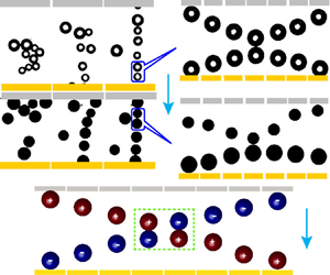
Figure 2(a) and supplementary movie 1 show the assemblage of a collection of non-conducting glass particles of different sizes in silicone oil under the influence of a DC field, in the set-up shown in figure 1(a). The experiment shows that, initially, the segregated particles tend to form a chain-like assembly between the electrodes under the influence of the electric field (Bonnecaze & Brady Reference Bonnecaze and Brady1992). Over a period of time, relatively stable and static chains are formed when adequate amounts of glass particles are accumulated between the electrodes. The particle assemblies within each chain undergo incessant to and fro oscillatory motions (refer to supplementary movie 1). Figure 2(b) and supplementary movie 1 show another interesting case wherein an assemblage of smaller glass particles and larger Ag-coated amberlite particles in silicone oil is investigated. The experiment shows that some of the larger Ag-coated amberlite particles migrate faster towards the electrodes to acquire charge at the initial stages of evolution. Subsequently, they help in assembling the glass and other Ag-coated amberlite particles after having repeated collisions between them. In fact, the progressive integration of the larger Ag-coated amberlite particles in the chain helps in increasing the packing density of the glass particles between the Ag-coated amberlite particles and the electrodes. Finally, a heterogeneous assembly composed of the bigger Ag-coated amberlite particles ‘chained’ by a collection of smaller glass particles of high packing density is formed.

Figure 2. Experimental time sequence micrographs depicting alignment of (a) a collection of glass particles, (b) a mixture of glass particles and Ag-coated amberlite particles, (c) Ag-coated amberlite particles and (d) uncoated amberlite particles under application of 6, 5, 5 and 6 kV cm $^{-1}$ average electric fields, respectively. The glass particles were
  $\sim$100
  $\mathrm {\mu }$m in diameter. The times indicated have units of seconds (s). The experiments were visualized under a microscope at 2.5
 $\times$ magnification. The images correspond to the top view of the particles.
The figures 2(c) and 2(d) and supplementary movie set 1 show that the phenomenon remains qualitatively similar when Ag-coated amberlite with a conducting surface and non-conductive amberlite (conductivity  ${\approx }10^{-10}$ S m
 $^{-1}$) particles are employed. In these motions, initially, the randomly placed microparticles move towards the nearest electrode where they undergo charge acquisition or reversal. Subsequently, the charged particles are attracted by the electrode of opposite polarity during which they start colliding with the other charged or uncharged particles. A few particles do not contact any other particle during the motions and thus continue their usual oscillation between the electrodes. During the formative stage of the chain, the Coulombic interaction of a charged particle with the bounding pair of charged particles of opposing polarity generates a motion of relatively higher frequency, as it is previously observed for a single particle oscillation between a pair of electrodes (Drews et al. Reference Drews, Cartier and Bishop2015). In fact, a small chain of charged particles also oscillates between the bounding pair of charged particles (or charged chains) of opposing polarity, in the similar manner, as the particles do.
Concisely, figure 2 uncovers a host of interesting phenomena displayed by multiple charged particles inside a microparticle-laden fluid flow.
4.1. Single particle phenomena
The results shown in figure 2 have multiple layers of scientific information, which are rather difficult to comprehend at one go. Thus, in order to elucidate the origin of such migrations of the charged particles inside a microparticle-laden fluid flow, a series of experiments have been performed involving either a single particle or a pair of particles. We initiate the discussions with the motions of single particles under an electric field with conducting and non-conducting surfaces. The experimental time sequence snapshots of a silver coated (Ag-coated) and an uncoated amberlite resin particle of  $\sim$500
  $\mathrm {\mu }$m radius each, under application of a 9 kV cm
 $^{-1}$ average electric field, are demonstrated in figures 3(a) and 3(b), respectively. The oscillatory motion of the conductive Ag-coated particle is expected and studied in earlier literature (Drews et al. Reference Drews, Kowalik and Bishop2014, Reference Drews, Cartier and Bishop2015). However, the uncoated amberlite particle also shows similar oscillatory behaviour, as shown by figures 3(b) and 3(e). This observation is particularly interesting, given the fact that the conductivity of the uncoated amberlite particle is rather limited (
 ${\sim } 10^{-10}$ S m
 $^{-1}$). Figure 3(c) demonstrates the simulated time sequence snapshots of a 500
  $\mathrm {\mu }$m radius conductive particle under application of a 9 kV cm
 $^{-1}$ average electric field.

Figure 3. Time sequence snapshots of (a) a Ag-coated and (b) an uncoated, amberlite resin particle of  $\sim$500
  $\mathrm {\mu }$m radius each under application of a 9 kV cm
 $^{-1}$ average electric field. (c) Simulated time sequence snapshots of a 500
  $\mathrm {\mu }$m particle under application of a 9 kV cm
 $^{-1}$ average electric field. The time indicated above each micrograph has unit of seconds (s). The plot (d) shows the variations of the charging time (
 $t_{ch}$) of a
  $\sim$500
  $\mathrm {\mu }$m radius amberlite resin particle coated with different materials with the average applied electric field. The error bars represent the maximum standard deviations obtained from five sets of experiments. The plot (e) shows the variations of the positions of the centres (
 $h$) of the particles from the bottom electrode at
  $z=0$, with time (
 $t$) corresponding to (a), (b) and (c). The broken (solid) lines correspond to the experimental (simulated) values, respectively. The experiments were visualized under a microscope at 2.5
 $\times$ magnification. The image panels shown in (a) and (b) correspond to the top view of the particles.
This experiment raises an important question on the mechanism which causes the reversal of the direction of the particles immediately after contact. In this regard, a collisional rebound may be thought of as one of the possibilities. However, the Stokes number (ratio of particle inertia to viscous forces),  $St(=\frac {1}{9}({{\rho _s}/{\rho _f}})Re_s)$ (where
  $Re_s={\rho _s D_s U_i}/{\mu _f}$ and
  $D_s$ and
  $U_i$ denote particle diameter and impact velocity, respectively), for the experiments reported here, is found to be
  $O(10^{-3})$. Prior-art (Joseph et al. Reference Joseph, Zenit, Hunt and Rosenwinkel2001; Birwa et al. Reference Birwa, Rajalakshmi, Govindarajan and Menon2018; Ruiz-Angulo, Roshankhah & Hunt Reference Ruiz-Angulo, Roshankhah and Hunt2019) suggests that below a critical value of
  $St\hspace {1mm}(\sim 10)$ the particles may not rebound after collision. Hence, any possibility of rebound due to an electrode–particle elastic collision can be safely ignored. The more probable reason can be that the non-conductive amberlite particles too undergo some charge transfer during contact with the electrodes, in a fashion similar to the Ag-coated conductive particles.
Figure 3(d) demonstrates the experimentally evaluated values of average charging time ( $t_{ch}$) of an amberlite particle (
 $r_s$,
  $\sim$500
  $\mathrm {\mu }$m) during contact with the electrodes. The results are reported for the particles coated with different materials and at different electric fields (
 $E_0$). Two additional types of particles, a conductive Ni-coated (nickel-coated) and a non-conductive Fe-coated (iron-coated) particle, were experimented with to get an approximate knowledge of the oscillatory trends shown by different materials. The Fe-coated particles were kept for two days at room temperature to reduce their conductivity due to oxidation. Figure 3(d) shows that both the conductive Ag-coated and Ni-coated particles show shorter charging times (
 $t_{ch}$) at the electrodes compared with the non-conductive Fe-coated and uncoated particles. In these experiments,
  $t_{ch}$ was evaluated by noting the difference in the time of zero approach velocity and the same for a marginal rebound velocity. The experiments suggest that the electrical conductivity of the particle at the surface has a significant influence on the charging time of the particles at the electrodes. Figure 3(e) shows the experimental trajectories of the Ag-coated and uncoated particles corresponding to figures 3(a) and 3(b), respectively.
Figure 3(e) also shows the numerically simulated trajectories in the geometry shown in figure 1(b), which is very similar to the experimental set-up shown in figure 1(a). It may be noted that in the simulations the particles were modelled as conductive. The dimensions shown in the schematic diagram of the computational domain in figure 1(b) were used for all the simulations, unless otherwise stated. The surrounding liquid and the particles were assigned physical properties similar to those mentioned for the experiments in § 2, unless otherwise stated. The particles were assigned the simulated theoretical values of charge given in figure 4(a), which depicts the charge acquired by a conductive particle in contact with the electrode, unless otherwise stated.

Figure 4. (a) The variation of the net charge ( $q$) acquired by amberlite particles of
  $\sim$500
  $\mathrm {\mu }$m radius, coated with a variety of materials, with the average applied electric field. The solid (hollow) symbols denote the experimental (numerical) values, respectively. The error bar represents the the maximum standard deviations obtained from five sets of experiments. (b) The variation of the simulated values of dimensionless drag coefficient (
 $\lambda _d$) with the dimensionless position (
 $h/r_s$) of a particle (
 $r_s=500$
  $\mathrm {\mu }$m) moving between two electrodes 5 mm apart. Here,
  $h$ is the position of the centre of the particle measured from the lower electrode at
  $z=0$.
It can be inferred from figure 3(e) that the motion of the uncoated particle is slightly sluggish compared with the Ag-coated particle. The numerically simulated trajectory again predicts higher particle speeds than both the uncoated and Ag-coated particles. The reason behind this trend can be better understood from figure 4(a), which depicts the average charge ( $q$) acquired by the particles at different values of average applied electric field (
 $E_0$). The method to calculate charge from the experiments is given in § 1.4 of the supplementary material. The drag force on the particles was experimentally estimated using the numerically simulated values of drag coefficient across the channel as depicted in figure 4(b). The hollow symbols in 4(a) correspond to the numerically simulated values of charge, which are approximately equal to the theoretical charge
  $Q_0$ described above. The Ag-coated and the Ni-coated particles are found to acquire
  $\sim$73 % while the Fe-coated and uncoated particles are found to contain
  $\sim$48 % of the theoretical value of charge
  $Q_0$. As the uncoated particle acquires less charge compared with the Ag-coated particles, and both the particles acquire significantly less charge compared to the theoretical values, they are acted upon by less electric force compared with the simulated particle. Hence, the experimental trajectories show sluggish behaviour compared with the numerical one.
4.2. Two-particle phenomena
Figures 5(a) and 5(b) demonstrate the experimental time sequence snapshots of Ag-coated amberlite resin particle pairs moving inside a liquid medium under application of a 9 kV cm $^{-1}$ average electric field. The videos of these motions have been summarized in supplementary movie 2. The image panel in (a) shows a pair of equal-sized particles of
  $\sim$550
  $\mathrm {\mu }$m radius each, while the smaller particle in (b) is
  $\sim$400
  $\mathrm {\mu }$m. The trajectories in the image panel (a) suggest that the particles, after reversal of charge at the respective electrodes after contact, move towards the electrodes of opposite polarity. During the motion, they appear to undergo an ‘elastic’ collision with each other before reversing their directions of motion. The behaviour is found to be very similar for the set-up with particles having different sizes in the image panel (b), with differences in the location of the point of contact and the path length of oscillations of the individual particles. In such a scenario, the prior-art suggests the possibility of the presence of a thin fluid layer between the particles (Birlasekaran Reference Birlasekaran1991; Joseph et al. Reference Joseph, Zenit, Hunt and Rosenwinkel2001; Khayari & Perez Reference Khayari and Perez2002; Drews et al. Reference Drews, Kowalik and Bishop2014, Reference Drews, Cartier and Bishop2015; Birwa et al. Reference Birwa, Rajalakshmi, Govindarajan and Menon2018; Ruiz-Angulo et al. Reference Ruiz-Angulo, Roshankhah and Hunt2019).

Figure 5. Experimental time sequence snapshots of two Ag-coated particles of (a) equal sizes of  $\sim$550
  $\mathrm {\mu }$m radius each (b) unequal sizes with radii of the smaller and bigger particles being
  $\sim$400 and
  $\sim$550
  $\mathrm {\mu }$m, respectively, under application of 9 kV cm
 $^{-1}$ average electric field. The time indicated above each micrograph has units of milliseconds (ms). Variations of the positions of the centres (
 $h$) of the particles measured from the lower electrode at
  $z=0$, with time (
 $t$) for the image panels shown in (a) and (b). Experimental time sequence snapshots of two uncoated particles of (d) equal sizes of
  $\sim$550
  $\mathrm {\mu }$m radius each (e) unequal sizes with radii of the smaller and bigger particles being
  $\sim$400 and
  $\sim$550
  $\mathrm {\mu }$m, respectively, under application of 9 kV cm
 $^{-1}$ electric field. (
 $f$) Variations of the positions of the centres (
 $h$) of the particles with time (
 $t$) for the image panels shown in (d) and (e). The evenly broken (unevenly broken) lines correspond to the case of equal (unequal) sized particles, respectively. The suffix S (B) correspond to the smaller (bigger) particles, respectively. The experiments were visualized under a microscope at 2.5
 $\times$ magnification. The image panels shown in (a), (b), (d) and (e) correspond to the top view of the particles.
Figure 5(c) demonstrates the trajectories shown by the particle pairs in (a) and (b). The trajectories are reported in terms of positions of the centres ( $h$) of the particles measured from the lower electrode at
  $z=0$, as a function of time (
 $t$). Figures 5(a) and 5(c) clearly indicate that the equal-sized particle pairs show a rather synchronized oscillatory behaviour. They approach each other with nearly similar speeds until the middle of the channel. After collision, they maintain reasonably the same speed of separation during their reverse motions. Figures 5(b) and 5(c) show that for the unequal-sized particles, the smaller particle accelerates after contact whereas the bigger particle moves rather sluggishly. Interestingly, the motions of the uncoated particles, shown in figures 5(d)–5(f) and supplementary movie 2, are found to be very similar to the Ag-coated particles, as shown in figures 5(a)–5(c).
Further interesting behaviours are observed when particles of two different types are used. For example, the oscillation characteristics of a Ag-coated amberlite particle and an uncoated particle under a 9 kV cm $^{-1}$ electric field are shown in figure 6(a–d). Again, as observed in figure 5, the smaller amberlite particle hastens its speed of return towards the electrode after collision, while the bigger Ag-coated particle moves rather slowly after contact, as shown in figure 6(a) and supplementary movie 3. This behaviour is more clearly indicated in the position versus time plots depicted in figure 6(d). In comparison, in the case of a bigger uncoated particle and a slightly smaller Ag-coated particle, the trajectories of the motion of the particles are found to be rather symmetric, as shown in figures 6(b) (and supplementary movie 3) and 6(d). For the combination of a Ag-coated particle and an uncoated amberlite particle of equal size figures 6(c) and 6(d) depict very marginal acceleration of the amberlite particle and deceleration of the Ag-coated particle after contact.

Figure 6. Experimental time sequence snapshots of a Ag-coated and an uncoated particle of (a) unequal sizes with radii of the smaller uncoated and bigger Ag-coated particles being  $\sim$400 and
  $\sim$550
  $\mathrm {\mu }$m, respectively, (b) unequal sizes with radii of the smaller Ag-coated and bigger uncoated particles being
  $\sim$450 and
  $\sim$550
  $\mathrm {\mu }$m, respectively, and (c) almost equal sizes of
  $\sim$550
  $\mathrm {\mu }$m radius each, under application of a 9 kV cm
 $^{-1}$ average electric field. The time indicated above each micrograph has units of milliseconds (ms). (d) Variations of the positions of the centres (
 $h$) of the particles measured from the lower electrode at
  $z=0$, with time (
 $t$), for the image panels shown in (a–c). Superscripts A, B and C in the legend indicate the particles shown in (a), (b) and (c), respectively, and Am corresponds to the uncoated particle and Ag corresponds to the Ag-coated particle. The black (yellow) rectangle represents the positive electrode (grounded electrode). The experiments were visualized under a microscope at 2.5
 $\times$ magnification. The image panels shown in (a), (b) and (c) correspond to the top view of the particles.
The experiments with equal-sized Ag-coated particles shown in figure 5(a) are qualitatively similar to that reported in previous studies (Mersch & Vandewalle Reference Mersch and Vandewalle2011; Bishop et al. Reference Bishop, Drews, Cartier, Pandey and Dou2018). Bishop et al. (Reference Bishop, Drews, Cartier, Pandey and Dou2018) observed that two equal conductive particles undergo electric-field-driven elastic collisions with redistribution of charge on their surfaces, keeping the total charge conserved. In addition to this, the results presented above reveal that (i) even non-conductive and dissimilar (a conductive and a non-conductive) particles and (ii) unequal-sized similar or dissimilar particles also undergo such field-driven collisions with charge reversals. To gain more insight into the nature of such field-driven collisions, quantitative estimations of charge contained by the particles before and after collisions are necessary. Figure 7(a–d) shows the variations of the average velocities ( $v_s$) and the fraction of the initial charge retained by the particles after collisions (
 $q^{*}$) as functions of the average electric field intensity (
 $E_0$) for different combinations of particles. Figures 7(a) and 7(b) refer to two equal-sized Ag-coated and uncoated particles, each with a radius of
  $\sim$550
  $\mathrm {\mu }$m each. Both the figures suggest that the velocities of approach and separation in the case of equal-sized particles remain reasonably similar as the particles retain approximately the initial amount of charge of opposite polarity after collision. Thus, the equal-sized particles undergo elastic collisions irrespective of the particle type. Figures 7(c) and 7(d) show the variations of unequal-sized Ag-coated and uncoated particles, respectively. As discussed in figures 5 and 6, figures 7(c) and 7(d) show that the velocities of the smaller particles increase and that of the bigger particles decrease after collision. The bigger particle retains almost 30–40 % of its initial charge, while the smaller particle retains approximately 120–150 %. The dotted (dashed) line refers to the separation velocity of the bigger (smaller) particle, predicted by elastic collision theory. It can be seen that
  $v_s$ of the smaller particle resembles the elastic collision velocities, but
  $v_s$ of the bigger particle is substantially less compared with the elastic collisions. Thus, it can be inferred that (i) equal-sized particles of similar type undergo ‘elastic’ electric-field-driven collisions and (ii) the collisions between unequal-sized particles are essentially ‘inelastic’.

Figure 7. Variation of the average velocity ( $v_s$) of the particles and the fraction of the initial amount of charge retained after collision (
 $q^{*}$) with average electric field (
 $E_0$) for (a) equal-sized Ag-coated particles with radius
  $\sim$550
  $\mathrm {\mu }$m each, (b) equal-sized uncoated particles with radius
  $\sim$550
  $\mathrm {\mu }$m each, (c) unequal-sized Ag-coated particles with the radius of the smaller being
  $\sim$400
  $\mathrm {\mu }$m and that of the bigger being
  $\sim$550
  $\mathrm {\mu }$m, and (d) unequal-sized uncoated particles with the radius of the smaller being
  $\sim$400
  $\mathrm {\mu }$m and that of the bigger being
  $\sim$550
  $\mathrm {\mu }$m. In panels (c and d), the notations specify the following:
  $P_{B{\_}b}$ (
 $P_{S{\_}b}$), velocities of bigger (smaller) particle before collision;
  $P_{B{\_}a}$ (
 $P_{S{\_}a}$), velocities of bigger (smaller) particle after collision;
  $q_{B{\_}a}$ (
 $q_{S{\_}a}$), fraction of the initial charge retained by the bigger (smaller) particle after collision;
  $E_{B{\_}a}$ (;
 $E_{S{\_}a}$), velocity of the bigger (smaller) particle after elastic collision between them.
We further explore some of the other interesting characteristics of the charge reversal for a set of two-particle systems. For this purpose, we report the magnified time sequence experimental snapshots during the charge reversals of two particles, under application of 5 kV cm $^{-1}$ average electric field, in figure 8(a–c). The image panel in figure 8(a) denotes two equal-sized Ag-coated particles of
  $\sim$550
  $\mathrm {\mu }$m radius each, while figure 8(b) corresponds to two equal-sized uncoated amberlite particles of the same size, as mentioned above. Figure 8(c) captures the dynamics of a Ag-coated (darker shade) and an uncoated amberlite (lighter shade) particle of
  $\sim$550
  $\mathrm {\mu }$m radius each. It can be inferred from figure 8(a–c) and supplementary movie 4, that both the particles in each panel show synchronized motions before and after collisions in all cases. The positively charged upper particle (returning from the positive upper electrode) first shows apparent contact with the negatively charged bottom particle (returning from the grounded electrode), after which both the particles reverse their trajectory, as demonstrated in figures 5 and 6. The time periods for charge reversals of the particles last for
  $10^{-2}-10^{-1}$ s. However, it may be noted here that such time measurements reported are not exact due to experimental artefacts, such as optical aberrations, while capturing the videos.

Figure 8. Experimental time sequence snapshots show the contact dynamics of (a) two Ag-coated, (b) two uncoated and (c) a Ag-coated and an uncoated particle of  $\sim$550
  $\mathrm {\mu }$m radius each under application of a 5 kV cm
 $^{-1}$ average electric field. The time indicated below each micrograph has units of milliseconds (ms). (d) Variations of the time periods for charge reversals (
 $t_c$) for the particle pairs shown in panels (a–c) with the average applied electric field. The experiments were visualized under a microscope at 10
 $\times$ magnification. The image panels shown in (a), (b) and (c) correspond to the top view of the particles. The dashed lines in the image panels of (a–c) indicate the initial positions of the particles during their close approach with each other.
Figure 8(d) shows the variations of the time period for charge reversals ( $t_c$) for the particle pairs shown in 8(a–c). The plot suggests that for all the three cases shown in 8(a–c),
  $t_c$ decreases with increasing field intensity, suggesting that the charge reversal kinetics during collision is directly proportional to the applied electric field. A higher value of electric field thus provides a greater driving force for rapid charge transfer between the particles. Experiments suggest that, at high electric fields, the local enhancement of electric field between the particles becomes progressively higher as they approach each other. This provides a relatively higher driving force for charge transfer, leading to shorter
  $t_c$, as illustrated in the computational study by Flittner & Přibyl (Reference Flittner and Přibyl2017) for the case of an oscillating droplet. Further, figure 8(d) suggests that the uncoated particles show slightly higher contact times than the Ag-coated particles. The Ag-coated particles with greater amounts of surface charge compared with the uncoated particles are expected to be subjected to greater local field enhancements during their collision. This may be a possible reason for the smaller
  $t_c$ than the corresponding uncoated particles.
The image panels in figure 9(a–d) and corresponding supplementary movie 5 depict the flight of two unequal-sized particles inside a liquid medium under a 5 kV cm $^{-1}$ electric field. The time sequence experimental snapshots in panel (a) correspond to Ag-coated particles of which the radius of the bigger particle is
  $\sim$550
  $\mathrm {\mu }$m and the smaller particle is
  $\sim$450
  $\mathrm {\mu }$m. Panel (b) shows the response for uncoated particles of approximately the same size as those in (a). Panels (c) and (d) depict bigger (smaller) Ag-coated (uncoated) particles. It is interesting to note that the contact dynamics shown by the unequal-sized particles is remarkably different from that observed in the case of equal-sized particles discussed above in figure 8. Figure 9 depicts that, even after the contact, the bigger particle carrying a larger amount of charge continues its motion while in contact with the smaller particle for a brief period before reversing its direction towards the oppositely charged electrode. The smaller particle, however, reverses its direction of motion almost immediately after the charge reversal.

Figure 9. Experimental time sequence snapshots of (a) two unequal-sized Ag-coated, (b) two unequal-sized uncoated, (c) a bigger Ag-coated and smaller uncoated and (d) a smaller Ag-coated and a bigger uncoated amberlite resin particles under application of a 5 kV cm $^{-1}$ average electric field. The time indicated below each micrograph has units of milliseconds (ms). The radii of the big and small particles are
  $\sim$550 and
  $\sim$450
  $\mathrm {\mu }$m, respectively. The experiments were visualized under a microscope at 10
 $\times$ magnification. The images correspond to the top view of the particles. The dashed lines in the image panels of (a–d) indicate the initial positions of the bigger particles during their close approach with the smaller ones.
In view of these observations, the ‘inelastic’ collision characteristics of significantly different sized particles can be summarized as (a) the bigger particle, after its engagement with the smaller particle approaching from the opposite direction, briefly continues its motion in the original direction along with the smaller particle, at a much reduced speed (images (ii)–(iv) of each panel); (b) the smaller particle then detaches itself from the union and reverses its direction of motion at a slightly higher speed than that of its approach (images (iv)–(vii); (c) after its disengagement from the smaller particle, the bigger particle still continues its flight towards the smaller particle for a very brief period of time (images (vi) and (vii)) before finally reversing its direction towards the opposite electrode; and (d) the bigger particle exhibits a much smaller speed after colliding with the smaller one. The experiments shown so far suggest that the charge reversal mechanisms between a pair of equal- or unequal-sized particles are very different. While it is observed that the equal-sized particles temporarily freeze for a very brief period of time, during the anticipated charge reversal (figure 8a–c), the unequal-sized particles form a union and move briefly along the direction of the bigger particle, during which the charge reversal is expected to take place.
In fact, the multi-particle PLFF systems shown in figure 2 also show such pair-wise repeated ‘elastic’ and ‘inelastic’ collisions inside the liquid medium, for equal- and unequal-sized particles. With the progress in time, a combination of these types of pair-wise motions and charge reversals during the collision lead to the large-scale assemblage of the particles inside a liquid medium. The charged particles keep showing this pair-wise oscillatory behaviour with repeated reversal of motions after charge reversals until there are some void spaces available during the chain formation.
4.3. Numerical investigations
The experiments on the pairs of equal- and unequal-sized particles, shown in figures 5–9, uncover the following key details: (a) the equal-sized particles acquire charge of nearly equal quantity of opposite sign; (b) there is a disparity of charge acquired by unevenly sized particles with the smaller particle getting overcharged and the bigger particle getting undercharged after a collision. In order to obtain a physical explanation of such observations on the charge reversal and subsequent motions of the particle pairs, a set of numerical simulations were carried out using parameters that largely emulate the experimental conditions. The model employed a system of two particles suspended in a liquid medium to qualitatively uncover the salient features of the oscillatory motions between a pair of electrodes under electric field. The results shown here help in identifying the underlying mechanism of the formation of particle chains, as shown previously in figure 2.
In the first simulation, a pair of uniformly sized particles oscillating between two parallel electrodes is considered, as schematically shown in the figure 1(b). The simulated time sequence snapshots shown in figures 10(a) and 10(b), along with supplementary movie 6, demonstrate the response of two equal-sized particles 1 (negatively charged) and 2 (positively charged) of 500  $\mathrm {\mu }$m radius each, under a 9 kV cm
 $^{-1}$ electric field for
  $q_{2t}=1$ and
  $q_{2t}=0.5$, respectively. Here,
  $q_{2t}$ is defined as the ratio of surface charge density of the particle 2 to its theoretical value. Figure 10(a) shows the variation of the positions of the centres (
 $h$) of particles 1 and 2, measured from the electrode at
  $z=0$, with time, under a 9 kV cm
 $^{-1}$ electric field for different values of
  $q_{2t}$. It can be inferred from the plot (a) that for
  $q_{2t}=1$, when the particles contain equal and opposite charge, the displacements of the particles from their initial positions are similar. The negatively charged particle moves towards the positively charged anode, while the positively charged particle migrates towards the cathode.

Figure 10. Time sequence snapshots of two equal-sized particles 1 and 2 of 500  $\mathrm {\mu }$m radius each, under application of a 9 kV cm
 $^{-1}$ average electric field for (a)
  $q_{2t}=1$ and (b)
  $q_{2t}=0.5$. Here,
  $q_{2t}$ represents the ratio of charge (
 $q$) contained by particle 2 to the theoretical value of charge. Particle 1 contains the theoretical value of charge of opposite sign. The time indicated above each micrograph has units of milliseconds (ms). The solid lines in the image panels of (a) and (b) indicate the initial positions of the particles during their close approach with each other. (c) The positions of the centres of two particles (
 $h$) measured from the bottom electrode at
  $z=0$, with time for different values of
  $q_{2t}$. The upper (black) graphs correspond to particle 1 and the lower (red) graphs correspond to particle 2. The inset plot represents the variation of
  $h$ of particle 2 during the initial time. The simulations were carried out employing an axisymmetric domain.
This synchronized motion of equal-sized particles is qualitatively confirmed from the experimental trajectory plots depicted in figures 5–8. For  $q_{2t}=0.5$, wherein particle 2 contains half the amount of charge contained by particle 1, figures 10(b) and 10(c) demonstrate that the trajectories are not similar. Particle 1, containing higher charge, shows expected motion towards the oppositely charged electrode. In contrast, particle 2, containing less charge, follows particle 1 for a brief period of time before migrating towards the oppositely charged lower electrode. Thus, the results in the simulated image set (b) is found to be very similar to the experimental results involving the unevenly sized particles in figures 5, 6 and 9. This observation leads to a reasonable confirmation that, during the process of dynamic charge reversals of the particles of unequal sizes, the charge distribution is rather unequal. The bigger particle shows a relatively slower motion after the ‘inelastic’ collision because it gains relatively less charge of opposite polarity.
Figure 11(a,b) demonstrates the simulated time sequence snapshots of a bigger particle 1 (negatively charged) and a smaller particle 2 (positively charged) of radii 500 and 400  $\mathrm {\mu }$m, respectively, under a 9 kV cm
 $^{-1}$ electric field for
  $q_{1t}=1$ and
  $q_{1t}=0.2$, respectively. Here,
  $q_{1t}$ represents the ratio of charge contained by particle 1 to the theoretical value of charge. Particle 2 contains the theoretical amount of charge in all the cases. In the first case, wherein the smaller particle 2 contains a lower magnitude of charge compared with particle 1, similar results are obtained as previously shown in figure 10(b). The negatively charged particle 1 rapidly moves towards the positively charged upper electrode, while the positively charged particle 2 follows particle 1 for a very brief period of time, before migrating towards the grounded electrode. However, experiments contradict this observation, thus suggesting that the bigger particle contains a smaller amount of charge after the collision. This result is further validated by the observations shown in figure 11(b) along with supplementary movie 7, where the bigger particle contains 20 % of the theoretical value of charge. In this case, in line with the experimental observations shown in figure 9, the bigger particle follows the smaller one for a brief period of time before reversing its direction.

Figure 11. Simulated time sequence snapshots of two unequal-sized particles 1 and 2 of radii 500 and 400  $\mathrm {\mu }$m, respectively, under application of a 9 kV cm
 $^{-1}$ average electric field for (a)
  $q_{1t}=1$ and (b)
  $q_{1t}=0.2$. Here,
  $q_{1t}$ represents the ratio of charge (
 $q$) contained by particle 1 to the theoretical value of charge. Particle 2 contains the theoretical amount of charge of opposite sign. The time indicated above each snapshot has units of milliseconds (ms). The solid lines in the image panels of (a) and (b) indicate the initial positions of the particles during their close approach with each other. (c) The positions of the centres of the two particles (
 $h$) measured from the bottom electrode at
  $z=0$, with time for different values of
  $q_{1t}$. The upper (black) graphs correspond to particle 1 and the lower (blue) graphs correspond to particle 2. The inset plot represents the variation of
  $h$ of particle 1 during the initial time. The simulations were carried out employing an axisymmetric domain.
Figure 11(c) demonstrates the variations of the positions of the centres of the two particles ( $h$) measured from the electrode at
  $z=0$, with time for different values of
  $q_{1t}$. The inset plot shows that particle 1 shows motion towards particle 2 only if the net charge on particle 1 is less than that of 2. The plots suggest that the larger the difference between the charges on the particles, the greater is the distance traversed by particle 1 in the direction of particle 2. Another key observation is that as the charge on 1 decreases, the speed of particle 2 increases, although the magnitude of charge on particle 2 remains constant. This observation is qualitatively similar to the experimental observations shown in figures 5 and 6 where the smaller particles show slight increment in speed compared with their original after charge reversal.
Figure 12 compares the simulated velocities of Ag-coated particles with the experimental ones shown in figure 7. Figure 12(a) shows that in the case of the equal-sized particles, the simulated velocities predict the experimental ones with reasonable accuracy. It may be noted here that charge assigned to each particle was  $Q_0$. In the case of the unequal-sized particles, based on the observations made in figure 7(c,d), the simulated particles were assigned
  $Q_0$ charge before collision, and after collision the charge assigned to the bigger particle was
  $0.35Q_0$ and that to the smaller particle was
  $1.35Q_0$. With these assigned values of charges, figure 12(b) shows that the simulated values of
  $v_s$ mimic the experimental values very well. The slight differences between the experimental and simulated values may be attributed to factors such as (i) the effect of low but finite liquid conductivity is not included in the simulations in which the liquid is assumed to be non-conductive, (ii) the effect of gravity is ignored in the simulations, (iii) the particles in the experiments are not perfect conductors as assumed in the simulations and (iv) there are inaccuracies associated with assignment of values of parameters such as liquid viscosity, particle charge and liquid permittivity in the simulations.

Figure 12. Variation of the average velocity ( $v_s$) of the particles with average electric field (
 $E_0$) for (a) equal-sized Ag-coated particles with radius 550
  $\mathrm {\mu }$m each and (b) unequal-sized Ag-coated particles with the radius of the smaller being 400
  $\mathrm {\mu }$m and that of the bigger being 550
  $\mathrm {\mu }$m. In panel (a), the dotted lines refer to simulated velocities. In panel (b), the notations specify the following:
  $P_{B{\_}b}$ (
 $P_{S{\_}b}$), velocities of bigger (smaller) particle before collision;
  $P_{B{\_}a}$ (
 $P_{S{\_}a}$), velocities of bigger (smaller) particle after collision;
  $P_{B{\_}sim{\_}b}$ (
  $P_{S{\_}sim{\_}b}$), simulated velocities of bigger (smaller) particle before collision;
  $P_{B{\_}sim{\_}a}$ (
 $P_{S{\_}sim{\_}a}$), simulated velocities of bigger (smaller) particle after collision.
Figures 13(a) and 13(b) demonstrate the experimental time sequence snapshots of two Ag-coated particles under 8 and 5 kV cm $^{-1}$ electric fields, respectively. The diameters of the big and small particles are
  $\sim$550 and
  $\sim$450
  $\mathrm {\mu }$m, respectively. The image panels (a) and (b) show that the average displacement of the bigger particle towards the smaller particle under two different electric fields is rather similar. However, in the case of the lower electric field, as shown in (b), the contact time between the particles as well as the time of retraction of the bigger particle is much higher compared with the higher electric field situation demonstrated in (a). This behaviour is intuitive for lower field values as charge reversal kinetics is expected to be slow, leading to an ‘inelastic’ collision with a higher contact time. The sluggish return of the bigger particle can be attributed directly to the lower value of electric force acting on it at lower field intensity. These observations are qualitatively confirmed by the simulated values of the variations of the positions of the centres of a negatively charged (400
  $\mathrm {\mu }$m) particle 1 and a positively charged (500
  $\mathrm {\mu }$m) particle 2 (
 $q_{2t}=0.5$) with time at different applied electric field intensities, as demonstrated in figure 13(c). The inset plot in (c) clearly demonstrates that, while the bigger particle 2 undergoes similar displacement towards the smaller particle 1 at all studied field strengths, the time of flight of particle 2 increases with decreasing field.

Figure 13. Experimental time sequence snapshots of Ag-coated amberlite resin particles under application of (a) 8 kV cm $^{-1}$ and (b) 5 kV cm
 $^{-1}$ average electric fields. The time indicated below each micrograph has units of milliseconds (ms). The diameters of the big and small particles are
  $\sim$550 and
  $\sim$450
  $\mathrm {\mu }$m, respectively. The experiments were visualized under a microscope at 10
 $\times$ magnification. The images correspond to the top view of the particles. The dashed lines in the image panels of (a and b) indicate the initial position of the bigger particle during its close approach with the smaller one. (c) Simulated values of the variations of the positions of the centres (
 $h$) measured from the lower electrode at
  $z=0$ of a 400
  $\mathrm {\mu }$m particle 1 and a 500
  $\mathrm {\mu }$m particle 2 with time (
 $t$), at different applied electric field intensities. The upper (blue) graphs correspond to particle 1 and the lower (red) plots correspond to a particle 2. The inset plot represents the magnified view of the positions of particle 2 during the initial time period. The simulations were carried out employing an axisymmetric domain.
Having discussed the origins of the oscillatory behaviours of the particles alongside their charge reversal dynamics under electric field, we now shift our focus to explore some of the important factors that drive the proposed phenomena. Figures 14(a) and 14(b) demonstrate the simulated distribution of the  $z$-component of the Maxwell stress tensor (
 $\boldsymbol {\tau }_z$) over two equal-sized particles 1 (negatively charged) and 2 (positively charged) of 500
  $\mathrm {\mu }$m radius each, under application of a 9 kV cm
 $^{-1}$ average electric field. Here, particle 1 is assigned the theoretical amount of charge. Figure 14(c) demonstrates that the magnitude of the Coulomb force (
 $F_C$) acting on the particles is very large compared to the dielectrophoretic force (
 $F_D$), and thus the former almost entirely contributes to the electrical forces acting on the particles. Figure 14(a) correspond to
  $q_{2t}=1$, wherein both the particles contain equal charge of opposite polarity. The images suggest that the negatively charged particle 1 experiences an attractive force towards the anode, while the positively charged particle 2 experiences a pull towards the cathode. This eventually leads to the separation of the particles from each other.

Figure 14. Simulated time sequence snapshots of the distribution of the  $z$-component of the Maxwell stress tensor (
 $\boldsymbol {\tau }_z$) over two equal-sized particles 1 and 2 of 500
  $\mathrm {\mu }$m diameter under application of a 9 kV cm
 $^{-1}$ average electric field for (a)
  $q_{2t}=1$ and (b)
  $q_{2t}=0.5$. Here,
  $q_{2t}$ represents the ratio of charge contained by particle 2 to its theoretical value of charge. Particle 1 contains the theoretical values of charge. The time indicated above each snapshot has units of milliseconds (ms). (c) Variations of the Coulomb force (
 $F_{C}$) and the dielectrophoretic force (
 $F_{D}$) acting at points
  $1^{t}$ and
  $2^{b}$ with time. The simulations were carried out employing an axisymmetric domain.
In order to obtain more in-depth information regarding the distribution of electric force on the particles, we consider points  $1^{t}(2^{t})$ at the topmost point of particle 1 (particle 2) and
  $1^{b}(2^{b})$ at the bottom-most point of particle 1 (particle 2), respectively. It may be noted here that the usage of the words ‘top’ and ‘bottom’ is only directed towards describing the results because the gravitational influence has been neglected in the formulation. Figure 15(a), corresponding to the case shown in figure 14(a), depicts the variation of
  $\boldsymbol {\tau }_z$ with time at the topmost and bottom-most points of the two particles. It can be seen from the plot that the top pole of particle 1 experiences a strong attractive force towards the anode, while the bottommost point experiences a weak attractive force towards particle 2. This facilitates the net movement of the particle towards the anode. On the other hand the bottom pole of particle 2 experiences a strong attractive force towards the cathode, while the topmost point experiences a weak attractive force towards particle 1. This facilitates the net movement of the particle towards the cathode. In a nutshell, when the particles carrying opposing charges of equal magnitude move in close proximity under an electric field, they experience a mutual attraction as well as an attractive force towards the electrodes of opposite polarity. While the brief association during the charge reversal is caused by the particle–particle attractive force, they move apart towards the electrodes owing to the larger particle-electrode attractive force.

Figure 15. Variations of the  $z$-component of the Maxwell stress tensor (
 $\boldsymbol {\tau }_z$) at the topmost and bottom-most points of two equal-sized particles 1 and 2 of 500
  $\mathrm {\mu }$m diameter under a 9 kV cm
 $^{-1}$ electric field for (a)
  $q_{2t}=1$ and (b)
  $q_{2t}=0.5$. Here,
  $q_{2t}$ represents the ratio of charge contained by particle 2 to its theoretical value of charge. Particle 1 contains the theoretical values of charge. The subscripts
  $t$ and
  $b$ in the legends denote the topmost and bottom-most points of particles 1 and 2 corresponding to figure 14. (c) Surface plot showing the variations of the magnitude of the electric field intensity (
 $E$) and (d) variations of
  $E$ along a cut line passing through the centres of particles 1 and 2 (axis of symmetry shown in figure 1b) at an average applied field intensity of 9 kV cm
 $^{-1}$, corresponding to the case shown in figure 14(a). (e) Surface plot showing the variations of
  $E$. (
 $f$) Variations of
  $E$ along a cut line passing through the centres of particles 1 and 2 (axis of symmetry shown in figure 1b) at an average applied field intensity of 9 kV cm
 $^{-1}$, corresponding to the case shown in figure 14(b). The colour scale in panels (c and e) from blue to red indicates increasing magnitude of
  $E$. The simulations were carried out employing an axisymmetric domain.
Figure 15(c) depicts the distribution of electric field magnitude ( $E$) along a cut line passing through the centres of the particles (axis of symmetry shown in figure 1b). The plots show that the electric field magnitude is highest at the topmost part of particle 1 and the bottom-most part of particle 2, which increases as the particles approach the respective electrodes. Thus, points
  $1^{t}$ and
  $2^{b}$ experience larger attractive forces from the electrodes, which progressively increase as the particles move towards them. The electric field in the gap between the particles gradually decrease as the particles move apart, indicating reduction in the mutual attraction between the particles.
Figure 14(b) demonstrates the simulated distribution of the  $z$-component of the Maxwell stress tensor (
 $\boldsymbol {\tau }_z$) over particles 1 and 2 for
  $q_{2t}=0.5$, wherein particle 2 contains half of the charge contained by particle 1 of opposite polarity. In this situation, the negatively charged particle 1 experiences a pull towards the positive electrode, while the positively charged particle 2 containing less charge briefly experiences a pull towards particle 1 and moves along its direction. The distributions of the stress due to electric field on the topmost and bottom-most points of particles 1 and 2, depicted in figure 15(b), reveal that the positive upward force acting on point
  $2^{t}$ is significantly larger than the downward force acting on point
  $2^{b}$ during the initial time period when the particles arrive at near proximity, and eventually decrease with increase in the separation distance. Thus, particle 2 briefly moves towards particle 1, before reversing its motion towards the oppositely charged electrode. The variation of the magnitude of electric field corresponding to this situation is depicted in figure 15(e, f), which suggests a significant increment of electric field between the particles during their close proximity. The electric field in the gap decreases as the particles move apart, leading to the decrease in the upward force experienced by
  $2^{t}$ compared with the downward force experienced by
  $2^{b}$ thus causing it to move away from the other particle. In this case, contrary to the case for
  $q_{2t}=1$,
  $1^{b}$ experiences a significantly larger downward force compared with the upward force experienced by
  $1^{t}$, during their close proximity, for a very brief period of time. However, particle 1 still experiences a larger net positive force, which causes it to move towards the upper electrode.
The simulated results shown in figures 14(b) and 15(b) can be summarized as follows: when two particles carrying unequal amounts of charge of the opposite polarity, are placed in close proximity under the influence of an externally applied electric field, the particles experience mutual attraction towards each other and towards the respective electrodes of opposite polarity. When their separation distance is small, the attraction experienced by the particle of less charge towards the particle of higher charge is larger than its attraction towards the electrode of opposite polarity. Thus, the particle of lower charge follows the particle of higher charge briefly, until the separation between them increases to the extent that it experiences more attractive force towards the electrode of opposite polarity, after which the particle starts moving towards the electrode. The net force on the particle of greater charge always acts towards the electrode of opposite polarity and it moves towards the electrode.
To summarize the above discussed cases, we present two model simulations shown in supplementary movies 8 and 9. Movie 8 depicts the motion of particle 1 (initially positively charged) and particle 2 (initially negatively charged) under a 9 kV cm $^{-1}$ electric field. On contact with each other they undergo charge transfer, which is modelled using an arbitrary rate constant to mimic the experimental time scales. Post charge transfer, they retain equal charge of opposite polarity and, under the influence of the externally applied field, they move apart in a synchronized manner. This simulation is qualitatively similar to the experimental motions of equal particles shown in supplementary movie 2. Movie 9 depicts the motion of a smaller particle 1 (initially positively charged) and a bigger particle 2 (initially negatively charged) under the application of a 9 kV cm
 $^{-1}$ average electric field. In this case post contact and charge transfer, while particle 1 retains the initial charge magnitude of opposite polarity, particle 2 retains only 20 % of initial charge of opposite polarity. Thus, it can be seen travelling in the direction of 1 for a brief period of time, before reversing its direction. This simulation emulates the experimental motions of unequal particles shown in supplementary movies 2 and 3.
4.3.1. Flow patterns and role of fluid properties
Thus far, the major focus of the discussion has been to elucidate the motions of the particles inside the liquid medium under an electric field. In this direction, the surrounding liquid medium is found to play a key role. For example, the dielectric contrast at the liquid–particle interface decides the capacity of the particles to retain charges, which is a crucial factor in determining the extent of Coulombic force experienced by them. Further, formation of interesting flow patterns can also be envisaged during their periodic approach and reversal of the spherical particles between the electrodes. Such flow patterns may not only be important in deciding the speeds of particle migration, however; they may also help in deciding the directions of the particle motion. In such a scenario, the viscosity of the liquid is expected to play a crucial role especially when the particles sizes are different.
Figures 16 and 17 show the velocity and streamline fields in the surrounding liquid medium at the various stages of migration of a pair of equal- and unequal-sized particles under electric field, respectively. The plots suggest that, as the spherical particles move in the confined space between the electrodes, they entrain the liquid surrounding them. Subsequently, high fluid velocities are observed near the front and rear ends of the particles, as shown in the first three frames of the image sets (a) and (c) of figures 16 and 17. The liquid velocity between the particles increases as the particles approach each other with the increase in their speed. In the process, the liquid between drains out and during the collision the ejection of the liquid happens at a relatively higher velocity. Following this, once the particles separate and move towards the electrodes, they again entrain liquid with them until they collide with the electrodes, as shown by the frames after collision of the image sets (a) and (c) of figures 16 and 17.

Figure 16. Simulated time sequence snapshots of (a) fluid velocity and (b) streamline fields for viscosity of the fluid  $\mu _{rf}=0.01$ Pa.s. (c) Fluid velocity and (d) streamline fields for viscosity of the fluid
  $\mu _{rf}=0.1$ Pa.s. The particles considered are of equal size with radius of 500
  $\mathrm {\mu }$m each. The other parameters used for the simulations are
  $E_0=9$ kV cm
 $^{-1}$ and
  $\varepsilon _{rf}=3$. The time indicated above the snapshots has units of milliseconds. The velocities indicated by the colour scales have units of ms
 $^{-1}$.

Figure 17. Simulated time sequence snapshots of (a) fluid velocity and (b) streamline fields for viscosity of the fluid  $\mu _{rf}=0.01$ Pa.s. (c) Fluid velocity and (d) streamline fields for viscosity of the fluid
  $\mu _{rf}=0.1$ Pa.s. The particles considered are of unequal sizes with the radius of the bigger particle being 550
  $\mathrm {\mu }$m and the smaller being 400
  $\mathrm {\mu }$m. The other parameters used for the simulations are
  $E_0=9$ kV cm
 $^{-1}$ and
  $\varepsilon _{rf}=3$. The time indicated above the snapshots has units of milliseconds. The velocities indicated by the colour scales have units of ms
 $^{-1}$.
Once the particles attain the steady to and fro oscillatory motion between the electrodes, a pair of counter-rotating circulation loops are found to appear across the particles near their equatorial regions. The arrows on the streamline plots denote the directions of the liquid flows in the zones of recirculations. In such a situation, the local stagnation points appear at the centres of the loops, where the liquid velocities nearly vanish, as shown in the image sets (b) and (d) of figures 16 and 17. As the particles move towards or away from each other, a stagnation point develops at the axial region between the particles, with the liquid around it moving in opposite directions. Examining the streamline plots for  $\mu _{rf}=0.01$ Pa.s and
  $\mu _{rf}=0.1$ in figures 16 and 17, it can be seen that the circulation loops are centred much closer to the particles in the case of
  $\mu _{rf}=0.01$ Pa.s compared with
  $\mu _{rf}=0.1$ Pa.s. Interestingly, the recirculation zones are of similar size, for a very synchronized motion of the particles with an ‘elastic’ collision in the middle. However, if an ‘inelastic’ collision takes between unequal-sized particles, the sizes and shapes of the recirculation zones in the surrounding liquid medium are asymmetric, as shown in figure 17(b,d). Further, a comparison between the images of figure 17(b,d) suggests that the recirculations near the electrodes are also suppressed for the high-viscosity case, and the velocity of liquid ejection between the particle and electrode is smaller (figure 17b,d). The results also suggest that the multi-particle assemblages shown in figure 2 are expected to have an array of such flow patterns around the particles while undergoing incessant to and fro motion between the electrodes.
Apart from the flow structures in the surrounding liquid, the viscosity of the fluid also influences the kinetics of the particle migration. For example, figures 16 and 17 show that the velocities of particle oscillations decrease with increase in the liquid viscosity, due to an increase in the hydrodynamic drag force. Interestingly, the point of collision can also be modulated by tuning the viscosity of the liquid. Figure 20(a) shows the variations of the positions ( $h$) of two unequal particles with time for two different liquid viscosities. The figure suggests that as the liquid viscosity increases, the point of collision shifts upwards. With the increase in viscosity of the liquid medium, the drag force experienced by each of the particles increases, with the electrical force acting on them remains constant. In the case of the smaller particle, for
  $\mu _{rf}=0.1$ Pa.s, due to an increase in the viscous drag, the net force acting downwards decreases more compared with the net upward force experienced by the bigger particle. Hence, the smaller particle travels a shorter distance downwards before its collision with the bigger particle. This, in turn, shifts the point of collision slightly upwards for
  $\mu _{rf}=0.1$ Pa.s. compared with
  $\mu _{rf}=0.01$ Pa.s.
Vorticity ( $\boldsymbol {\omega }=\boldsymbol {\nabla }\times \boldsymbol {v}_f$) fields show the local fluid rotation or spinning near a point. Figure 18 shows the azimuthal vorticity (
 $\omega _\theta ={\partial v_{fr}}/{\partial z}-{\partial v_{fz}}/{\partial r}$) fields, for equal-sized particles, where
  $v_{fr}$ and
  $v_{fz}$ denote the
  $r$ and
  $z$ directional fluid velocities, respectively. Figure 19 denotes the vorticity fields for unequal-sized particles. At the surface of the solid, the fluid velocity goes to zero (no-slip condition), which results in very high velocity gradients in the regions surrounding the particles, leading to the generation of vorticity in the fluid. Figures 18 and 19 show that regions of strong positive and negative vorticity develop in the liquid in the immediate vicinity of the particles. Interestingly, the first three frames of the image sets shown in figures 18 and 19 show a common-flow-up configuration (CFUp) of twin vortices accompanying the bottom particle during its motion towards the top particle (Lu & Zhai Reference Lu and Zhai2019). Again in the same set of images, the vortices surrounding the top particle show a common-flow-down arrangement (CFDn) during its motion towards the bottom one. This can be more explicitly understood by the arrows on the first three frames of image sets (b) and (d) of figures 16 and 17. Importantly, the 2nd, 3rd and 4th frames of the image sets (a) and (b) of figures 18 and 19 (and the corresponding images on figures 16 and 17) suggest that after the collision there is a reversal of the direction of the rotations in the vortices. In such a situation, the top particle moving towards the top electrode is accompanied by a pair of CFUp vortices, whereas the bottom one is surrounded by a pair of CFDn vortices until it arrives the bottom electrode. In the case of the unequal-sized particles, after the collision, the smaller particles travels faster towards the top electrode and, for a brief period of time, both the particles travel downwards. Thus, the last images of the image sets shown in figure 19 depict negative vorticity fields around both the particles. It can be seen from both figures 18 and 19 that the magnitudes of vorticity are higher for
  $\mu _{rf}=0.01$ Pa.s compared with
  $\mu _{rf}=0.1$ Pa.s. This is because the velocity gradient in the lower viscosity fluid near the solid is greater than the higher viscosity fluid.

Figure 18. Simulated time sequence snapshots of azimuthal vorticity ( $\omega _\theta$) fields for (a) viscosity of the fluid
  $\mu _{rf}=0.01$ Pa.s. and (b) viscosity of the fluid
  $\mu _{rf}=0.1$ Pa.s. The particles considered are of equal size with radius of 500
  $\mathrm {\mu }$m each. The other parameters used for the simulations are
  $E_0=9$ kV cm
 $^{-1}$ and
  $\varepsilon _{rf}=3$. The time indicated above the snapshots has units of milliseconds. The
  $\omega _\theta$ values indicated by the colour scales are normalized with the maximum values. For
  $\mu _{rf}=0.01$ Pa.s, the values are normalized by
  $\omega _\theta =6\times 10^{4}$ s
 $^{-1}$, and, for
  $\mu _{rf}=0.1$ Pa.s, the values are normalized by
  $\omega _\theta =3000$ s
 $^{-1}$.

Figure 19. Simulated time sequence snapshots of azimuthal vorticity ( $\omega _\theta$) fields for (a) viscosity of the fluid
  $\mu _{rf}=0.01$ Pa.s. and (b) viscosity of the fluid
  $\mu _{rf}=0.1$ Pa.s. The particles considered are of unequal sizes with the radius of the bigger particle being 550
  $\mathrm {\mu }$m and the smaller being 400
  $\mathrm {\mu }$m. The other parameters used for the simulations are
  $E_0=9$ kV cm
 $^{-1}$ and
  $\varepsilon _{rf}=3$. The time indicated above the snapshots has units of milliseconds. The
  $\omega _\theta$ values indicated by the colour scales are normalized with the maximum values. For
  $\mu _{rf}=0.01$ Pa.s, the values are normalized by
  $\omega _\theta =8\times 10^{4}$ s
 $^{-1}$, and, for
  $\mu _{rf}=0.1$ Pa.s, the values are normalized by
  $\omega _\theta =5000$ s
 $^{-1}$.
Another point of difference in the  $\omega _\theta$ fields is that they are much diffused in the case of
  $\mu _{rf}=0.1$ Pa.s compared with
  $\mu _{rf}=0.01$ Pa.s. The vorticity transport equation can be written as
  ${\partial \boldsymbol {\omega }}/{\partial t}+(\boldsymbol {v}_{f}\boldsymbol {\cdot }\boldsymbol {\nabla })\boldsymbol {\omega }= (\boldsymbol {\omega }\boldsymbol {\cdot }\boldsymbol {\nabla })\boldsymbol {v}_{f}+\nu \nabla ^2 \boldsymbol {\omega }$, where
  $\nu$ refers to the kinematic viscosity of the fluid. The second term on the left-hand side of the equation denotes the convection of vorticity, while the second term of the right-hand side of the equation refers to the diffusion of vorticity with diffusivity,
  $\nu$. Since the fluid velocities are much less, the convection of vorticity can be ignored. Thus, the vorticity is transported from the regions near the surface of the solid mainly by diffusion. The length scale of the diffusion can be defined as
  $\sim \sqrt {\nu t}$. Thus, for
  $\mu _{rf}=0.1$ Pa.s,
  $\nu$ is greater compared to
  $\mu _{rf}=0.01$ Pa.s. Also, the time for diffusion is greater due to lower velocity in the case of
  $\mu _{rf}=0.1$ Pa.s. Thus, the vorticity is transported to a larger distance compared with
  $\mu _{rf}=0.01$ Pa.s, and the
  $\omega _\theta$ fields in the case of
  $\mu _{rf}=0.1$ are more diffused compared with
  $\mu _{rf}=0.01$ Pa.s.
Finally, the relative permittivity ( $\varepsilon _{rf}$) of the fluid is another important parameter affecting the oscillation characteristics of the particles. Generally, relative permittivity in conjunction with the fluid conductivity are more important in determining the particle dynamics. But in the present study the fluid medium is considered as non-conductive. Hence, the variation of fluid conductivity is not considered. Figures 20(b) and 20(c) show the positions (
 $h$) of the particles with time for varying values of
  $\varepsilon _{rf}$. Figure 20(b) denotes the case of equal-sized particles, and figure 20(c) refers to unequal-sized particles with the smaller particle being at the top. Both the figures indicate that the velocities of the particles increase with increasing fluid permittivity. As
  $\varepsilon _{rf}$ increases, the electric field around the particle increases due to increasing bound charge density, leading to a greater Coulombic force acting on the particle. Thus, the particle speed is expected to increase in such circumstances.

Figure 20. Simulated variations of the positions of the centres of the particles ( $h$) from the lower electrode at
  $z=0$ with time (
 $t$) for (a) two unequal-sized particles with the radius of the bigger particle being 550
  $\mathrm {\mu }$m and the smaller being 400
  $\mathrm {\mu }$m for different values of
  $\mu _{rf}$, (b) two equal-sized particles with radius of 500
  $\mathrm {\mu }$m each and (c) two unequal-sized particles with the radius of the bigger particle being 550
  $\mathrm {\mu }$m and the smaller being 400
  $\mathrm {\mu }$m for different values of
  $\varepsilon _{rf}$. The other parameters used for (a) are
  $E_0=9$ kV cm
 $^{-1}$ and
  $\varepsilon _{rf}=3$. The other parameters used for (b) and (c) are
  $E_0=9$ kV cm
 $^{-1}$ and
  $\mu _{rf}=0.25$ Pa.s.
5. Applications
The experiments shown here can also be extended to a number of futuristic microfluidic applications. For example, the particle chains in a PLFF (e.g. figure 2) can also be formed inside a microchannel with the help of an externally applied electric field to cause an on-demand restriction or opening of the flow. Such motions of a chain of glass microparticles inside a microfluidic set-up are shown in figure 21 and supplementary movie 10. The details related to the fabrication of the channels can be found elsewhere (Dutta et al. Reference Dutta, Ghosh, Pattader and Bandyopadhyay2019). In these experiments, silicone oil suspended with glass particles was flown through the channel. The experiments uncover various stages of chain formation, which initiate with the collision and charging of a few glass particles with electrodes. Subsequently, the particles undergo oscillations between the electrodes and also between other particles. Some particles do not collide with the electrodes or other particles and escape to the downstream with the flow. Each collision between a pair of charged particles or between a pair of charged chains or between a charged particle and a chain lead to charge reversal of the colliding components, which sustains the to and fro motions of the particles or chains in the void space available within the chains. Over a period of time, such motions of the charged particles increase their packing density between the electrodes to form a ‘garland’ of glass particles between the electrodes (shown by arrows in figure 21b).

Figure 21. (a) Experimental time sequence snapshots of chaining of glass particles ( $\sim$10
  $\mathrm {\mu }$m radius) under application of a 12 kV cm
 $^{-1}$ average electric field, inside a 400
  $\mathrm {\mu }$m diameter microfluidic channel. (b) Experimental micrograph depicting the rotation of the chain of glass microparticles under application of a 12 kV cm
 $^{-1}$ average electric field, inside a 400
  $\mathrm {\mu }$m diameter microfluidic channel. The experiments were visualized under a microscope at 10
 $\times$ magnification. The images correspond to the top view of the particles. The arrow in panel (a) indicates the direction of the flow.
Remarkably, at a very high field intensity, the garland-like morphology is also found to show an anticlockwise unsteady stick-slip motion in which the Coulombic force active between the electrodes enables one half of the chained particles in the garland to move in the opposite direction of the other half. In fact, each of the two halves of the garland have opposite charge, which is reflected from their occasional joining due to the Coulombic attraction. In a way, the large collection of particles between the electrodes develop a pathway to electric field discharge. The discharge is less when the particles or the chains move, while the same is significant when the movements of the particles are sluggish or stationary. Most of the particle movements in the multi-particle experiments in figures 2 and 21 largely follow the various combinations of the two-particle motions described in the study. On the other hand, from the electrorheological point of view, the assemblage shown in figures 2 and 21 also hint towards the on-demand generation of localized power-law behaviours inside microfluidic systems under the guidance of an electric field.
6. Conclusions
We explore the pathways to the self-organization of a collection of microparticles inside a dielectric fluid under the influence of an external electric field. The electric is applied in such a manner that the electrodes are in direct contact with the fluid of significantly low electrical conductivity, which leads to the flow of a very weak leakage current through the fluid upon application of a high intensity field. In such a PLFF, embedding the particles of different size or surface conductivity effectively helps in improving the net capacitance of the fluid of low dielectric permittivity. Subsequently, the particles self-organize in the direction of the applied field, creating optimal channels for electric field discharge between the electrodes. The particles move when there is a build-up of potential difference, but they become stationary when the electric field discharges through them. A combined experimental and computational study provides an insight to the dynamics of such systems by considering a two-particle system undergoing oscillatory motions upon application of an electric field. The major observations are:
(i) Unlike the single-particle motion between a pair of electrodes, in the multi-particle system, the particles also gather charge during the collisions between themselves. Importantly, for such a system, the oscillatory to and fro motions of the particles are observed between a pair of particles, a pair of chains, a particle and a chain, an electrode and a particle, and between the electrodes. Charge transfer followed by charge reversal between the particles near contact are found to be the necessary driving forces for the reversal of the directions of motion.
(ii) The finer features of the multi-particle assemblage are explored by employing a model two-particle system. The experiments together with the numerical simulations for such systems uncover that the time of contact and charge reversal increase with reduction in the applied field intensity or the surface conductivity of the particles. The equal-sized particles exhibit a synchronized oscillatory pattern. Their speeds of approach prior to contact and the speeds of separation, subsequent to contact and charge reversal, are reasonably identical. Unequal-sized particles, on the other hand, show asymmetric trajectories, in such a manner that the speed of the smaller particle increases marginally after contact, while the bigger particle demonstrates a rather sluggish behaviour after contact. Experiments with unequal-sized particles also reveal that, after contact between the particles, the union of the particles moves in the direction of the bigger particle briefly before the charge reversal and separation of the particles take place. In these processes, the equal-sized particles undergo electric-field-driven ‘elastic’ collisions, while the collisions between unequal particles are rather ‘inelastic’.
(iii) Numerical simulations corroborate the experimental observations (a) when equal-sized particles contain equal and opposite amount of charges and (b) when, for unequal-sized particles, the bigger (smaller) particle contains a smaller (larger) amount of opposite charge, after collision. The distributions of the simulated electric force on the particles reveal that, in a pair of equal and oppositely charged particles, each particle experiences attraction towards the electrode of opposite polarity, which overcomes the mutual attraction between the particles. Thus, the particles move apart from each other, as also observed in the experiments. On the contrary, in the case of particles carrying unequal quantities of charge of opposite polarity, when the gap between the particles is small, the particle with less charge experiences more attractive force towards the particle of higher charge than the electrode of opposite polarity. This causes the particle to follow the particle of higher charge, until the attractive force between it and the electrode of opposite polarity overcomes its attraction towards the particle of higher charge. Periodic to and fro movements of the spherical particles facilitate the formation of the recirculation zones around each particle. An array of such flow patterns around each particle can be envisaged for a multi-particle system while they undergo incessant to and fro motion between the electrodes. The non-slipping particle–liquid interface ensures the generation of a very high velocity gradient in the liquid medium present near a moving particle, which eventually leads to the formation of the vortices in the liquid. In a way, the electrical energy supplied to the particles facilitates their mechanical motion which in turn dissipates through the formation of vortices in the surrounding liquid medium. The size and strength of the vortices around each particle, viscosity of the liquid medium, and the dielectric contrast across the liquid–particle interface play key roles in determining the particle speed, point of collision and trajectory of motion in a PLFF under electric field. The location and the number of vortices around a particle can be modulated by changing the particle size and viscosity of the surrounding liquid.
(iv) Experiments with the multi-particle system exhibit different kinds of assemblies, hinting at the onset of on-demand power-law electrorheological behaviour under the guidance of an electric field. Further, translating a similar system into a microfluidic channel with a unidirectional flow bias reveals the trapping of the microparticles between the electrodes.
Concisely, the study qualitatively uncovers various finer features of the oscillatory motions of particles in a liquid medium under an electric field. The results suggest that an in-depth analysis of the mechanisms of charge transfer, charge reversal between the particles, and the role of the flow patterns in the liquid medium on such phenomena can be potent areas of future research. The phenomena can also be harnessed for a number of futuristic applications, such as microfluidic vortex generators or flow control valves, on-demand catalyst beds for reaction engineering, extraction of solid from liquid and microrheology.
Supplementary material and movies
Supplementary material and movies are available at http://dx.doi.org/10.1017/jfm.2021.22.
Acknowledgements
We also thank the support from the computer centre for the supercomputing PARAM Ishan facilities at IIT Guwahati. Discussions with Dr D. Roy are also gratefully acknowledged.
Funding
We thank DST SERB, grant no. EMR/2016/001824 and MeitY-grant no. 5(9)/2012-NANO, Government of India, for financial aids.
Declaration of interests
The authors report no conflict of interest.


