


1. Introduction
Atmospheric winds and storms inject energy to large-scale oceanic geostrophic flows and near-inertial waves. It has long been known that wave–wave interactions can transfer energy from large scales to small scales (McComas & Bretherton Reference McComas and Bretherton1977) where waves break causing diapycnal mixing (Sun & Kunze Reference Sun and Kunze1999; Polzin & Lvov Reference Polzin and Lvov2017). Moreover, Lelong & Riley (Reference Lelong and Riley1991) have shown that geostrophic modes can act as a catalyst in moving energy amongst inertia–gravity waves of the same frequency, transferring wave energy from large scales to small. The catalysing effect in transferring energy of waves with the same frequency was also found in the rotating shallow-water system by Ward & Dewar (Reference Ward and Dewar2010), but, in this two-dimensional space, the frequency constraint prevents redistribution of energy among waves of different length scales. Similarly, Savva & Vanneste (Reference Savva and Vanneste2018) found that a random barotropic quasi-geostrophic flow can redistribute energy amongst internal tides of the same vertical structure and frequency. Understanding the formation of small-scale waves through nonlinear wave–wave interaction or wave–vortex interactions is not only of fundamental interest, but also provides a means by which to estimate the turbulence production rate (or mixing efficiency), since inertia–gravity wave breaking is a major source of diapycnal mixing in the ocean (MacKinnon et al. Reference MacKinnon, Zhao, Whalen, Waterhouse, Trossman, Sun, St. Laurent, Simmons, Polzin and Pinkel2017).
McComas & Bretherton (Reference McComas and Bretherton1977) coined the term ‘induced diffusion’ to describe the scattering of small-scale fast waves by larger-scale slow waves, and pointed out that ‘induced diffusion’ also occurs in the Wentzel–Kramers–Brillouin (WKB) setting with a random background flow. McComas & Bretherton (Reference McComas and Bretherton1977) outlined the derivation in the WKB setting in their appendix, though the derivation is not well justified. Kafiabad, Savva & Vanneste (Reference Kafiabad, Savva and Vanneste2019, hereafter Reference Kafiabad, Savva and VannesteKSV2019) gave a rigorous derivation of the diffusivity in the WKB setting by assuming that the large-scale velocity is weaker than the intrinsic group velocity of waves and employing a multi-scale analysis. The analysis in Reference Kafiabad, Savva and VannesteKSV2019 also applies to other wave systems; Bôas & Young (Reference Bôas and Young2020, hereafter Reference Bôas and YoungBY2020) adapted the analysis to deep-water surface waves. Each paper emphasizes that diffusion in wavenumber space occurs only transverse to the group velocity direction, meaning that wave action is scattered amongst wavenumbers on surfaces of constant frequency. This is consistent with the earlier studies on the scattering effect of inertia–gravity waves by geostrophic modes mentioned above. By contrast, both Barkan, Winters & McWilliams (Reference Barkan, Winters and McWilliams2017) and Thomas & Arun (Reference Thomas and Arun2020) have recently demonstrated frequency spreading and a forward cascade of wave energy in numerical studies of the interaction between geostrophic turbulence and near-inertial waves. Although the present paper only tiptoes into these waters, these numerical observations serve as partial motivation for the present study.
Reference Kafiabad, Savva and VannesteKSV2019 and Reference Bôas and YoungBY2020 both consider the evolution of a random spatially slowly varying background flow that is frozen in time, and proceed to analyse the WKB transport equation for wave action density ((2.1) below). The WKB approximation, however, is also consistent with a time-dependent flow, so long as the temporal variation is slow compared to that of the waves’ frequencies. In this paper, we generalize the multi-scale analysis of Reference Kafiabad, Savva and VannesteKSV2019 to unsteady large-scale flows, and show that this extra freedom turns out to allow scattering of waves across frequencies, or along the group velocity direction in spectral space, a process we term ‘frequency diffusion’. To connect this new finding to the results in Reference Kafiabad, Savva and VannesteKSV2019 and Reference Bôas and YoungBY2020, we introduce a similarity scaling of the velocity field, using the time scale of the velocity variation as a control parameter on the diffusivity. We find that diffusion in the group velocity direction is negligible if the unsteady large-scale flow evolves either too slowly (consistent with previous results) or too quickly, but has a peak for time scales comparable to the time needed for waves to travel across the dominant eddy scale.
We investigate this theoretical prediction by solving the ray-tracing equations for inertia–gravity waves in the rotating shallow-water system, with a time-varying synthetic mean flow. The mean flow is constructed by assuming that each wavenumber mode obeys an Ornstein–Uhlenbeck (OU) process, and demanding an energy spectrum that obeys a power law with slope  $-3$. By explicitly varying the decorrelation time scale, we show that, as predicted, wave action diffuses across surfaces of constant frequency, with a tendency to spread towards higher frequency. Notably, as wave action is conserved in the ray-tracing equations (Bretherton & Garrett Reference Bretherton and Garrett1968), this spread to higher (intrinsic) frequency implies a concomitant net increase of wave energy. This new wave energy is drawn from the mean flow.
2. Diffusion of wave action by unsteady velocity fields
We use the standard ray-tracing approximations for the linear evolution of waves on a slowly varying background flow  $\boldsymbol {U}$, i.e.
  $|\partial \boldsymbol {U}/\partial t| \ll |\boldsymbol {U}|\omega _r$ and
  $|\boldsymbol {\nabla }_{\!\boldsymbol {x}\,}\boldsymbol {U}| \ll |\boldsymbol {U}| |\boldsymbol {k}|$, where
  $\boldsymbol {k}$ is the wavevector and
  $\omega _r$ is the intrinsic frequency. Without wave–wave interactions the phase-space wave action density
  $a(\boldsymbol {x},\boldsymbol {k},t)$ then solves the linear transport equation
 \begin{equation} a_t + \boldsymbol{\nabla}_{\!\boldsymbol{k}\,} \omega \boldsymbol{\cdot} \boldsymbol{\nabla}_{\!\boldsymbol{x}\,} a - \boldsymbol{\nabla}_{\!\boldsymbol{x}\,} \omega \boldsymbol{\cdot} \boldsymbol{\nabla}_{\!\boldsymbol{k}\,} a=0, \end{equation}
where  $\omega = \omega _r + \boldsymbol {U}(\boldsymbol {x},t) \boldsymbol {\cdot } \boldsymbol {k}$ is the absolute frequency. The intrinsic frequency
  $\omega _r(\boldsymbol {k})$ is assumed to be independent of
  $\boldsymbol {x}$ and
  $t$. As is usual in ray tracing, the space–time coordinates
  $(\boldsymbol {x},t)$ are tuned to the wave envelope scales, so they are slow compared to the wavelength and frequency, and the background flow
  $\boldsymbol {U}(\boldsymbol {x},t)$ is allowed to vary on these envelope scales.
Following Reference Kafiabad, Savva and VannesteKSV2019 and Reference Bôas and YoungBY2020, we assume the weak current limit, i.e.  $|\boldsymbol {U}| \ll |\boldsymbol {c}|$, where
  $\boldsymbol {c}=\boldsymbol {\nabla }_{\!\boldsymbol {k}\,}\omega _r$ is the intrinsic group velocity. Specifically, we let the typical size of
  $|\boldsymbol {U}|/|\boldsymbol {c}|$ be
  $\varepsilon$, and define slow time and space variables
  $T = \varepsilon ^2 t$ and
  $\boldsymbol {X} = \varepsilon ^2 \boldsymbol {x}$, respectively. Unlike Reference Kafiabad, Savva and VannesteKSV2019 and Reference Bôas and YoungBY2020, however, we assume that the velocity field depends on the fast time and space variables, i.e.
  $\boldsymbol {U} = \boldsymbol {U}(\boldsymbol {x},t)$, instead of assuming that
  $\boldsymbol {U}$ is frozen on the fast time. We show in appendix A that, if
  $\boldsymbol {U}$ is a homogeneous and stationary random field, then (2.1) is approximated by
 \begin{equation} \partial_t a + \boldsymbol{c}(\boldsymbol{k}) \boldsymbol{\cdot} \boldsymbol{\nabla}_{\!\boldsymbol{x}\,} a = \boldsymbol{\nabla}_{\!\boldsymbol{k}\,} \boldsymbol{\cdot} ({\boldsymbol{\mathsf{D}}} \boldsymbol{\cdot}\boldsymbol{\nabla}_{\!\boldsymbol{k}\,}a). \end{equation}
Here we have reverted to the original  $(\boldsymbol {x},t)$ coordinates, and
  ${\boldsymbol{\mathsf{D}}}$ is a symmetric diffusion tensor with Cartesian components
 \begin{equation} {\mathsf{D}}_{ij} = {\mathsf{D}}_{ji} = - \tfrac{1}{2}k_nk_m \int_{-\infty}^{\infty} \partial_{x_i}\partial_{x_j} \, {\mathbb{E}} [ U_n(\boldsymbol{x},t)U_m(\boldsymbol{x}-\boldsymbol{c} s, t-s) ] \,\mathrm{d} s, \end{equation}
where summation over repeated indices is implied, and ensemble averaging is denoted by  ${\mathbb {E}}[\cdot ]$. This is equivalent to (2.4) of Reference Kafiabad, Savva and VannesteKSV2019, except for the retained fast time dependence in the velocity autocorrelation function
 \begin{equation} V_{nm}(\boldsymbol{r},\tau) = {\mathbb{E}} [U_n(\boldsymbol{x}+\boldsymbol{r},t+\tau)U_m(\boldsymbol{x},t)]. \end{equation}
As indicated, for homogeneous and stationary velocity fields, the function  $V_{nm}$ depends only on the space–time separations. The Fourier transform in
  $d$-dimensional space and time of a function
  $f(\boldsymbol {r},\tau )$ is
 \begin{equation} \hat{f}(\boldsymbol{q},\sigma) = \int_{\mathbb{R}}\int_{\mathbb{R}^d} \,f(\boldsymbol{r},\tau) \exp({-\textrm{i}(\boldsymbol{q} \boldsymbol{\cdot} \boldsymbol{r} + \sigma \tau)}) \,\mathrm{d}\boldsymbol{r} \,\mathrm{d} \tau. \end{equation}
 Throughout the paper, we will use  $\boldsymbol {k}$ for the wavenumber of the waves, and
  $\boldsymbol {q}$ for the wavenumber associated with mean flow quantities, with magnitudes
  $k=|\boldsymbol {k}|$ and
  $q=|\boldsymbol {q}|$, respectively. Using the inverse Fourier transform and the identity
  $\int _{-\infty }^\infty \textrm {e}^{\textrm {i} \sigma s} \,\textrm {d} s = 2{\rm \pi} \delta (\sigma )$, the diffusivity components can be formulated as
 \begin{equation} {\mathsf{D}}_{ij} = \frac{k_n k_m}{2(2{\rm \pi})^d} \int_{\mathbb{R}^d} q_i q_j \hat{V}_{nm}(\boldsymbol{q},-\boldsymbol{q} \boldsymbol{\cdot} \boldsymbol{c}(\boldsymbol{k}) ) \,\mathrm{d}\boldsymbol{q}. \end{equation}
For steady flows,  ${\mathsf{D}}_{ij}$ reduces to (A 7) of Reference Kafiabad, Savva and VannesteKSV2019 and (2.6) of Reference Bôas and YoungBY2020. However, for unsteady flows, there may be diffusion along the group velocity direction in spectral space, i.e.
  ${\boldsymbol{\mathsf{D}}}\boldsymbol {\cdot }\boldsymbol {c} \neq \boldsymbol {0}$. By the definition of
  $\boldsymbol {c}=\boldsymbol {\nabla }_{\!\boldsymbol {k}\,}\omega _r$, this implies diffusion of frequency values, as will be demonstrated below.
3. Diffusion by two-dimensional isotropic non-divergent velocity fields
We show here that frequency diffusion is non-zero for unsteady, non-divergent, isotropic random velocity fields. For a general time-dependent flow, the divergent part of the velocity field presumably also contributes to frequency diffusion, but a purely non-divergent flow is chosen here because of its simplicity and our interest in the effects of geostrophic modes on inertia–gravity waves. We also assume the domain is two-dimensional, and consider an isotropic dispersion relationship  $\omega _r = \omega _r(k)$, with
  $k = \sqrt {k_1^2+k_2^2}$, which holds for both inertia–gravity waves in the rotating shallow-water system and for deep-water waves. We introduce a random streamfunction
  $\psi$ such that
  $(U_1,U_2) = (-\partial _{x_2}\psi , \partial _{x_1}\psi )$. Letting
 \begin{equation} C(\boldsymbol{r},\tau) = {\mathbb{E}}[\psi(\boldsymbol{x} +\boldsymbol{r},t+\tau)\psi(\boldsymbol{x},t)], \end{equation}
we have the following relations:
 \begin{equation} \hat{V}_{11} = q_2^2\hat{C}, \quad \hat{V}_{22} = q_1^2\hat{C} \quad\mbox{and}\quad \hat{V}_{12} = \hat{V}_{21}= -q_1q_2\hat{C}. \end{equation}
Substituting these relations into (2.6), one finds
 \begin{equation} {\mathsf{D}}_{ij}(\boldsymbol{k}) = \frac{1}{2(2{\rm \pi})^2}\int q_i q_j [k^2q^2 - (\boldsymbol{k} \boldsymbol{\cdot} \boldsymbol{q})^2] \, \hat{C}(\boldsymbol{q}, -\boldsymbol{q} \boldsymbol{\cdot} \boldsymbol{c}(k)) \,\mathrm{d}\boldsymbol{q}. \end{equation}
 Hereafter, we assume that the spectrum of the correlation function  $C$ is isotropic, i.e.
  $\hat {C}(\boldsymbol {q},\sigma ) = \hat {C}(q,\sigma )$, where
  $q = |\boldsymbol {q}|$. It is then convenient to use two sets of polar wavenumber coordinates,
  $\boldsymbol {k} = k(\cos \theta ,\sin \theta )$ and
  $\boldsymbol {q} = q(\cos \eta ,\sin \eta )$, which yields
 \begin{gather} {\mathsf{D}}_{11} = \frac{1}{2(2{\rm \pi})^2} \int_0^{2{\rm \pi}}\!\int_0^\infty q^5 k^2 \cos^2(\eta + \theta)\sin^2\eta \,\hat{C}(q, -qc(k)\cos\eta) \,\mathrm{d} q \,\mathrm{d}\eta, \end{gather}
 \begin{gather}{\mathsf{D}}_{22} = \frac{1}{2(2{\rm \pi})^2} \int_0^{2{\rm \pi}}\!\int_0^\infty q^5 k^2 \sin^2(\eta + \theta)\sin^2\eta \,\hat{C}(q, -qc(k)\cos\eta) \,\mathrm{d} q \,\mathrm{d}\eta, \end{gather}
 \begin{gather}{\mathsf{D}}_{12} = \frac{1}{2(2{\rm \pi})^2} \int_0^{2{\rm \pi}}\!\int_0^\infty q^5 k^2 \sin(\eta + \theta)\cos(\eta + \theta)\sin^2\eta \,\hat{C}(q, -qc(k)\cos\eta) \,\mathrm{d} q \,\mathrm{d}\eta. \end{gather}
Here  $c(k)=|\boldsymbol {c}(k)|$. In polar coordinates the diffusivity matrix is diagonal and the radial diffusivity
 \begin{equation} {\mathsf{D}}^{\,p}_{11}(k) = \frac{\boldsymbol{k}\boldsymbol{\cdot}{\boldsymbol{\mathsf{D}}}\boldsymbol{\cdot}\boldsymbol{k}}{k^2} = \frac{k^2}{2(2{\rm \pi})^2}\int_0^{2{\rm \pi}} \!\int_0^\infty q^5 \hat{C}(q,-qc(k)\cos\eta) \sin^2\eta \cos^2\eta \,\mathrm{d} q \,\mathrm{d}\eta. \end{equation}
Similarly, the azimuthal diffusivity
 \begin{equation} {\mathsf{D}}^{\,p}_{22}(k) = \frac{k^2}{2(2{\rm \pi})^2} \int_0^{2{\rm \pi}} \! \int_0^\infty q^5 \hat{C}(q,-qc(k)\cos\eta) \sin^4\eta \,\mathrm{d} q \,\mathrm{d}\eta \quad\mbox{and}\quad {\mathsf{D}}^{\,p}_{12}=0. \end{equation}
In general,  $\hat {C}$ is real and non-negative because it is the Fourier transform of a covariance function. Hence for smooth
  $\hat {C}$ the diffusivity
  ${\boldsymbol{\mathsf{D}}}$ has two strictly positive eigenvalues. However, in the limiting case of a steady mean flow,
  $\hat {C}$ has a delta function in its second argument and then
  ${\mathsf{D}}^{\,p}_{11}=0$ but
  ${\mathsf{D}}^{\,p}_{22}>0$. This was the singular diffusion case considered by Reference Bôas and YoungBY2020.
The wave action equation (2.2) in polar wavenumber coordinates becomes
 \begin{equation} \partial_t a + \boldsymbol{c}(k) \boldsymbol{\cdot} \boldsymbol{\nabla}_{\!\boldsymbol{x}\,} a = \frac{1}{k} \partial_k (k{\mathsf{D}}^{\,p}_{11}\partial_k a ) + \frac{1}{k^2}{\mathsf{D}}^{\,p}_{22} \partial^2_\theta a. \end{equation}
This leads to an evolution equation for wave energy density  $e = \omega _r a$. In the case of non-dispersive waves, with
  $\omega _r = c_0k$ and
  $c_0$ being a constant, (3.5) implies
  ${\mathsf{D}}_{11}^{\,p} = bk^2$, where
  $b$ is some positive constant. Integrating
  $c_0k$ times (3.7) over phase space yields the total wave energy evolution equation
 \begin{equation} \frac{\textrm{d}}{\textrm{d} t} \int e k \,\mathrm{d} k \,\mathrm{d} \theta \,\mathrm{d}\kern0.7pt\boldsymbol{x} = b \int k\partial_k\left(k^3\partial_k \frac{e}{k}\right) \,\mathrm{d} k \,\mathrm{d} \theta \,\mathrm{d}\kern0.7pt\boldsymbol{x} = 3b\int e k \,\mathrm{d} k \,\mathrm{d}\theta \,\mathrm{d}\kern0.7pt\boldsymbol{x}, \end{equation}
after two integrations by parts. The total wave energy therefore increases exponentially with time at the  $k$-independent rate
  $3{\mathsf{D}}_{11}^{\,p}/k^2$.
We also note that, in this non-dispersive case, a source term  $Sk_f^{-1}\delta (k-k_f)$ on the right-hand side of (3.7) gives a steady-state wave energy spectrum
  $\int ek \,\mathrm {d}\theta \,\mathrm {d}\kern0.7pt\boldsymbol {x}$ proportional to
  $k^2$ for
  $k<k_f$, and constant for
  $k>k_f$.
3.1. Dependence of radial diffusivity on time scale of the velocity field
We exhibit the generic dependence of the radial diffusivity on the time scale of the velocity field by using a similarity solution for streamfunction. In particular, we let
 \begin{equation} \psi(\boldsymbol{x},t) \mapsto \psi(\boldsymbol{x},\alpha t), \end{equation}
where  $1/\alpha >0$ indicates how fast or slow the flow evolves. Then
 \begin{equation} C(\boldsymbol{r},\tau) \mapsto C(\boldsymbol{r},\alpha \tau) \quad\mbox{and}\quad \hat{C}(q,\sigma) \mapsto \frac{1}{\alpha} \hat{C}\left(q,\frac{\sigma}{\alpha} \right). \end{equation}
Correspondingly, the radial diffusivity becomes
 \begin{align} {\mathsf{D}}^{\,p}_{11} &= \frac{k^2}{(2{\rm \pi})^2}\int_0^{\rm \pi}\int_0^\infty q^5 \frac{1}{\alpha}\hat{C}\left(q, \frac{-qc(k)\cos\eta}{\alpha}\right) \sin^2\eta \cos^2\eta \,\mathrm{d} q \,\mathrm{d}\eta \nonumber\\ &= \frac{k^2} {(2{\rm \pi})^2} \int_0^\infty \int_{-1/\alpha}^{1/\alpha} q^5\hat{C}(q, -qc(k)z) \alpha^2 z^2\sqrt{1 - \alpha^2z^2} \,\mathrm{d} z \,\mathrm{d} q, \end{align}
where  $z = \cos (\eta )/\alpha$ in the second line. The behaviour of the radial diffusivity for fast and slow background flows can be investigated by taking the limits
  $\alpha \rightarrow \infty$ and
  $\alpha \rightarrow 0$, respectively.
For fast flows the radial diffusivity is approximately
 \begin{equation} {\mathsf{D}}^{\,p}_{11} \sim \frac{1}{\alpha} \frac{k^2}{32{\rm \pi}} \int_0^\infty q^5\hat{C}(q,0) \,\mathrm{d} q,\quad \mbox{as}\ \alpha \rightarrow \infty. \end{equation}
Here we have assumed that the spectrum  $\hat {C}(q,\sigma )$ is sufficiently steep at large
  $q$ such that the integral above converges. For slow flows one finds
  ${\mathsf{D}}^{\,p}_{11} \rightarrow 0$ as
  $\alpha \rightarrow 0$ (however, the exact order of
  ${\mathsf{D}}^{\,p}_{11}$ in terms of a power of
  $\alpha$ depends on the detailed form of
  $\hat {C}$). Thus, if the velocity field evolves too slowly or too quickly, the radial diffusivity goes to zero. Below, we investigate numerically the diffusivity in the full range of velocity time scales.
4. Numerical simulations of ray-tracing equations
We test our theoretical findings using numerical solutions of the ray-tracing equations
 \begin{equation} \frac{\textrm{d}\kern0.7pt\boldsymbol{x}}{\textrm{d} t} = \boldsymbol{U} + \boldsymbol{c} \quad\mbox{and}\quad \frac{\textrm{d}\boldsymbol{k}}{\textrm{d} t} = -(\boldsymbol{\nabla}_{\!\boldsymbol{x}\,}\boldsymbol{U}) \boldsymbol{\cdot} \boldsymbol{k}. \end{equation}
Notably, in the relevant case  $\boldsymbol {c}(\boldsymbol {k})$, these equations have an exact scaling symmetry: if
  $\boldsymbol {U}(\boldsymbol {x},t)$ is replaced by
  $\boldsymbol {U}(a\boldsymbol {x},at)$ with some scaling factor
  $a>0$ then (4.1a,b) are invariant under the rescaling
  $\boldsymbol {X}=a\boldsymbol {x}$ and
  $T=at$. For steady flows this means that the ray-tracing dynamics is self-similar for all choices of
  $a>0$ in
  $\boldsymbol {U}(a\boldsymbol {x})$, i.e. the length scale of the mean flow does not matter. For unsteady flows the self-similarity holds if the length and time scales of the mean flow are kept in fixed proportion.
We now specialize to inertia–gravity waves in the rotating shallow-water system, for which
 \begin{equation} \omega_r(k) = f (1 + L_d^2k^2 )^{1/2} \quad\mbox{and}\quad c(k) = \sqrt{gH} [(k L_d)^{-2} + 1 ]^{-1/2} \end{equation}
are the intrinsic frequency and group velocity magnitude, respectively. Here  $f$ is the Coriolis parameter,
  $g$ is gravitational acceleration,
  $H$ is the layer depth and
  $L_d = \sqrt {gH}/f$ is the deformation scale. We characterize the background flow by its magnitude
  $U_0$ and its length scale
  $L_0$, and define the Froude number
  $\mathit {Fr} = U_0/\sqrt {gH}$ and the Rossby number
  $\mathit {Ro} = U_0/(\,f\kern0.05emL_0)$. Choosing the scale of the mean flow to be
  $L_0=L_d$ sets
  $\mathit {Fr} = \mathit {Ro}$.
4.1. A model of stationary and homogeneous velocity field
We use a doubly periodic square domain of size  $L$ such that the spatial Fourier coefficients of a function
  $f(\boldsymbol {x},t)$ are
 \begin{equation} \tilde{f}_{\boldsymbol{q}}(t) = \int_{[0,L]^2}f(\boldsymbol{x},t)\,\textrm{e}^{-\textrm{i} \boldsymbol{q}\boldsymbol{\cdot} \boldsymbol{x}} \,\mathrm{d}\kern0.7pt\boldsymbol{x} \quad \mbox{for}\ \boldsymbol{q}=\frac{2{\rm \pi}}{L}(n_1,n_2),\quad n_1,n_2 \in \mathbb{Z}. \end{equation}
The streamfunction is modelled as
 \begin{equation} \psi(\boldsymbol{x},t) = \frac{1}{L^2}\sum_{\boldsymbol{q}}\tilde{\psi}_{\boldsymbol{q}}(t)\,\textrm{e}^{\textrm{i} \boldsymbol{q}\boldsymbol{\cdot}\boldsymbol{x}} \quad \mbox{where}\ \tilde{\psi}_{\boldsymbol{q}}(t) = L\sqrt{\frac{P(q)}{2}} [A_{\boldsymbol{q}}(t)+\textrm{i}B_{\boldsymbol{q}}(t) ], \end{equation}
where  $\psi _{\boldsymbol {q}}$ satisfies the reality condition
  $\tilde {\psi }_{\boldsymbol {q}}(t) = \tilde {\psi }^*_{-\boldsymbol {q}}(t)$, so we need to consider only
  $q_1 \geq 0$, say. The function
  $P(q)$ determines the energy spectrum, and
  $A_{\boldsymbol {q}}(t)$ and
  $B_{\boldsymbol {q}}(t)$ are real independent unit-variance OU processes satisfying (see e.g. Gardiner Reference Gardiner1985)
 \begin{equation} \textrm{d} A_{\boldsymbol{q}} = -\alpha A_{\boldsymbol{q}} \,\mathrm{d} t + \sqrt{2\alpha} \,\mathrm{d} W \quad\mbox{and}\quad \textrm{d} B_{\boldsymbol{q}} = -\alpha B_{\boldsymbol{q}} \,\mathrm{d} t + \sqrt{2\alpha} \,\mathrm{d} W', \end{equation}
where  $W$ and
  $W'$ are independent Wiener processes. Note that the use of the same symbol
  $\alpha$ here and in (3.9) is intentional: while here
  $\alpha$ is dimensional, in both places it scales time for the mean flow.
Stationarity is ensured by choosing the initial values  $A_{\boldsymbol {q}}(0)$ and
  $B_{\boldsymbol {q}}(0)$ to follow independent standard normal distributions. The autocovariances of the OU parameters are
  ${\mathbb {E}}[A_{\boldsymbol {q}}(\tau +t)A_{\boldsymbol {q}}(t)] = {\mathbb {E}}[B_{\boldsymbol {q}}(\tau +t)B_{\boldsymbol {q}}(t)] = \textrm {e}^{-\alpha |\tau |}$, and so from (3.1)
 \begin{equation} C(\boldsymbol{r},\tau) = \frac{1}{L^2}\sum_{\boldsymbol{q}}P(q)\exp({\textrm{i}\boldsymbol{q} \boldsymbol{\cdot} \boldsymbol{r}-\alpha |\tau|}). \end{equation}
 Using (2.5), the Fourier transform of  $C$ is then
 \begin{equation} \hat{C}(\boldsymbol{q},\sigma) = \int_{-\infty}^{\infty}\int_{[0,L]^2} C(\boldsymbol{r},\tau)\exp({-\textrm{i}\boldsymbol{q}\boldsymbol{\cdot}\boldsymbol{r}-\textrm{i}\sigma \tau}) \,\mathrm{d}\boldsymbol{r} \,\mathrm{d} \tau = P(q)\frac{2\alpha}{\sigma^2 + \alpha^2}. \end{equation}
The spectrum is set to a band-limited power spectrum of the form
 \begin{equation} P(q) = \left(\frac{2 U_0^2L^2}{\sum_{Q_1<q<Q_2} q^{2-n}}\right) q^{-n} \mathbbm{1}_{Q_1<q<Q_2}, \end{equation}
where  $\mathbbm {1}_{Q_1<q<Q_2}$ is the indicator function, being 1 within the specified range of
  $q$ and 0 outside. Using (3.2a–c), the prefactor in (4.8) ensures that the mean flow energy is
 \begin{equation} {\mathbb{E}} \left[\frac{|\boldsymbol{U}|^2}{2}\right] = \frac{1}{2L^2}\sum_{\boldsymbol{q}} q^2P(q) = U_0^2. \end{equation}
 Finally, using the expression for  $\hat {C}$ above and taking the continuum limit
  $L\rightarrow \infty$, the radial diffusivity (3.5) is
 \begin{equation} {\mathsf{D}}^{\,p}_{11} = \frac{4U_0^2 k^2} {\int_{\mathbb{R}^2}q^{2-n}\mathbbm{1}_{Q_1<q<Q_2} \,\mathrm{d}\boldsymbol{q}} \int_0^{\rm \pi}\!\int_{Q_1}^{Q_2} \frac{q^{5-n}\alpha}{q^2c(k)^2\cos^2\eta + \alpha^2} \sin^2\eta\cos^2\eta \,\mathrm{d} q \,\mathrm{d}\eta. \end{equation}
When  $\alpha \rightarrow 0$,
 \begin{equation} {\mathsf{D}}^{\,p}_{11} \sim \alpha k^2 \frac{U_0^2}{c^2}. \end{equation}
4.2. Radial spreading of energy
In this section, we present numerical results demonstrating frequency diffusion in spectral space. We integrate (4.1a,b) using a second-order Runge–Kutta time-stepping method. The spectral slope of the autocorrelation is set to  $n = 6$, which gives a one-dimensional energy spectrum with slope
  $-3$, and the limiting wavenumbers are
  $Q_1 = L_d^{-1}$ and
  $Q_2 = 50 L_d^{-1}$. The domain scale is
  $L = 8{\rm \pi} L_d$ and the model uses
  $512^2$ grid points to resolve the maximum and minimum wavenumbers, with the minimum wavenumber increment set to be as small as possible. The Rossby and Froude numbers are set to
  $\mathit {Ro} = \mathit {Fr} = 0.1$. The WKB approximation requires
  $|\boldsymbol {U}|^{-1}|\partial \boldsymbol {U}/\partial t| \sim \alpha \ll \omega _r$ and
  $|\boldsymbol {U}|^{-1}|\boldsymbol {\nabla }_{\!\boldsymbol {x}\,}\boldsymbol {U}| \sim L_d^{-1} \ll k$. From the dispersion relationship in (4.2a,b), the latter requires
  $kL_d\gg 1$ so that the first requirement is
  $\alpha \ll \omega _r \sim k\sqrt {gH}$.
Since the spectrum of the streamfunction is sufficiently steep and dominated by  $Q_1$, the typical length scale is approximately
  $1/Q_1 =L_d$ (this is also approximately the decorrelation length scale). The fast time scale is the time it takes for waves, moving at the group velocity, to traverse the dominant size of the eddies, or
  $L_d/c \approx L_d/\sqrt {gH}=1/f$. Thus, the slow time scale is approximately
  $1/(\,f\,\mathit {Fr}^2)$. For convenience, we define a non-dimensional time
  $t^* = ft$ and correlation
  $\alpha ^* = \alpha /f$. We compute the trajectories of 100 rays in physical and spectral space, up to time
  $t^* = 1/\mathit {Fr}^2$. For each run, all the rays are initially located uniformly in
  $[0,L]\times [0,L]$, with the same wavevector amplitude
  $k$ and initial intrinsic frequency
  $\omega _r$, but random angle
  $\theta$. We vary
  $\alpha ^*$ from
  $0$ to
  $100$, despite the fact that the larger values violate the WKB assumption.
Figure 1(a) shows a snapshot of a realization of the streamfunction  $\psi$. As mentioned earlier, the wavenumber spectrum of the streamfunction decreases sufficiently fast so that
  $\psi$ is dominated by large-scale features. Figure 1(b) shows trajectories of all the rays in physical space for a simulation with
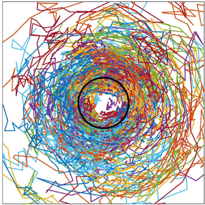
  $\alpha ^* = 1$, where the black box shows the size of the periodic domain for realizing the velocity field. Rays have travelled far away from their initial locations at the end of the simulation. Figure 2(c) shows the trajectories of rays in spectral space for this simulation. The rays not only spread outside of the initial ring (which shows the initial locations of rays in spectral space), but also spread inside of the ring, just like diffusion of a passive tracer.

Figure 1. (a) A snapshot of a realization of the streamfunction. (b) Trajectories of rays in physical space for  $\alpha ^*=1$ and
  $\omega _r(0) \approx 10f$, where the black square has length
  $L/L_d$.

Figure 2. Ray trajectories in spectral space for  $\alpha ^* = 0$, 0.1, 1 and 10 with
  $\omega _r(0) \approx 10f$.
The four panels of figure 2 show the ray trajectories in wavenumber space for simulations with  $\alpha ^*$ ranging from
  $0$ to
  $10$. For these runs, the initial
  $k$ is large enough so that the intrinsic group velocity is well approximated by
  $\sqrt {gH}$. Figure 2(a), with
  $\alpha ^*=0$, shows that, when the velocity field is steady, radial diffusion is very limited and rays are confined to a narrow annulus about the initial wavenumber. This is expected, since
  $\textrm {d}\omega /\textrm {d} t = 0$ for steady flows and
  $\omega \approx \omega _r$ under the weak current approximation, so deviations of the intrinsic frequency from its initial value are uniformly bounded in time by the Froude number. When
  $\alpha ^*$ increases from 0 to 1, rays spread faster and further away from their initial locations, indicating stronger radial diffusion. When
  $\alpha ^*$ increases further to 10, spreading in spectral space slows down, and radial diffusion becomes weaker compared to the case with
  $\alpha ^*=1$. Thus, figure 2 qualitatively verifies the theoretical predictions that frequency diffusion is very weak when the time scale of the velocity field is too large or too small. In addition, the simulations show that frequency diffusion achieves a maximum if
  $\alpha ^*= O(1)$.
Figure 3(a) shows the evolution of the intrinsic frequency averaged over all the rays for a short time window. The averaged intrinsic frequency,  $\bar {\omega }_r$, is proportional to the integration of intrinsic frequency over the spectral and physical domain if we assume that the action density on each ray is the same. As discussed in § 3,
  $\bar {\omega }_r$ increases with time approximately exponentially for large
  $k$ or in the high-frequency limit, which holds initially for all the rays and continues to hold for those rays not diffused to small
  $k$. For
  $\alpha ^* \neq 0$, the quantity
  $\ln [\bar {\omega }_r(t^*)/\bar {\omega }_r(0)]$ grows approximately linearly. We use the least-squares method to find the rate
  $\ln [\bar {\omega }_r(t^*)/\omega _r(0)]$ increases, denote the value by
  $\textrm {d}\ln [\bar {\omega }_r(t^*)/\omega _r(0)]/\textrm {d} t^*$, and use it as a measure of radial diffusivity for different
  $\alpha ^*$. Figure 3(b) shows that, among the simulations performed, radial diffusivity is largest for
  $\alpha ^*=1$. As predicted by the theory and demonstrated by figure 2, radial diffusivity is small when
  $\alpha ^*$ is too large or small. Of course, in reality the time scale of the background flow is determined by the flow itself. If we match
  $\alpha$ to the eddy turnover rate
  $\sqrt {{\mathbb {E}} (V_x-U_y)^2}$ in our simulations, then frequency diffusion occurs at approximately 50 % of its maximal value, as shown by the black dashed line in figure 3(b). Still, even at this weaker strength, the frequency diffusion is irreversible and leads to exponentially growing wave energy at long times. Interestingly, if
  $\alpha$ is matched to the eddy turnover rate, then at constant Froude number the spatial and temporal mean flow scales are in fixed proportion. In light of the comment below (4.1a,b), this means that the ray-tracing dynamics is then self-similar, so after a suitable rescaling of time the choice of
  $L_0$ does not matter.

Figure 3. (a) Evolution of  $\ln [\bar {\omega }_r(t^*)/\bar {\omega }_r(0)]$ for initial intrinsic frequency
  $\omega _r(0) \approx 10f$. (b) Dependence of
  $\textrm {d}\ln [\bar {\omega }_r(t^*)/\bar {\omega }_r(0)]/\textrm {d} t^*$ on
  $\alpha ^*$ for
  $\omega _r(0) \approx 10f$. (c) Evolution of
  $\ln [\bar {\omega }_r(t^*)/ \bar {\omega }_r(0)]$ for different
  $\omega _r(0)$. The black dashed line in (b) denotes the value of
  $\sqrt {{\mathbb {E}}\zeta ^2}/f$, where
  $\zeta =V_x-U_y$ is the vorticity of the background velocity field.
Asymptotically, if we use  $U_0/L_d$ as an estimation of
  $\alpha$ since the velocity field is dominated by a length scale
  $L_d$, we find
  $\alpha ^* = O(U_0/\sqrt {gH})=O(\mathit {Fr})$ (J. Vanneste, private communication). Furthermore, for sufficiently small
  $\mathit {Fr}$ flows such that approximation (4.11) applies,
  $k^2/{\mathsf{D}}^{\,p}_{11} = 1/(\,f\,\mathit {Fr}^3)$ is the frequency diffusion time scale. Note that this time scale is even longer than the slow time scale
  $1/(\,f\,\mathit {Fr}^2)$, which may explain why frequency diffusion was not observed in previous studies. For instance, Wagner, Ferrando & Young (Reference Wagner, Ferrando and Young2017) found azimuthal diffusion of internal tides propagating through a barotropic quasi-geostrophic flow in the
  $\mathit {Fr} = \mathit {Ro}$ regime, but they did not find noticeable frequency diffusion. They ran their simulations barely up to
  $t = O(1/(\,f\,\mathit {Fr}^3))$ and hence frequency diffusion is expected to be weak.
Figure 3(c) shows the dependence of  $\ln [\bar {\omega }_r(t^*)/\omega _r(0)]$ on initial intrinsic frequency. Overall,
  $\bar {\omega }_r$ increases faster for higher initial wave frequency. For the three runs, the WKB requirement of length scale separation and large-
 $k$ limit hold well for
  $\omega _r(0) \approx 10f$, but barely hold for
  $\omega _r(0) \approx 3.3f$. The result for near-inertial waves with
  $\omega _r(0) \approx 1.1f$ is also presented here. Although near-inertial waves modulated by geostrophic flows do not satisfy the WKB approximation due to its large horizontal scale, Kunze (Reference Kunze1985) and Young & Jelloul (Reference Young and Jelloul1997) found that wavevectors of near-inertial waves do obey a ray-tracing formula that contains the refraction term by the background flow in (4.1a,b). For
  $\omega _r(0) \approx 1.1f$,
  $\bar {\omega }_r$ also increases with time, despite the questionable validity of the large-
 $k$ limit and the weak current approximation. In fact, initially
  $\sqrt {{\mathbb {E}}|\boldsymbol {U}|^2} = 0.34|\boldsymbol {c}|$ and
  $\omega \approx \omega _r$ does not hold. In this case, conservation of absolute frequency does not prevent intrinsic frequency from shifting to higher frequency even for steady mean flow. Therefore, there is no reason to expect
  $\bar {\omega }_r$ not to change.
5. Conclusions
We have considered wave action diffusion in spectral space induced by a time-dependent mean flow under the WKB approximation, with the assumption that the background mean flow is weak compared to the intrinsic group velocity of the waves. In addition to the previously found wave action diffusion along constant-frequency surfaces in wavenumber space, we find that for time-dependent flows diffusion also occurs across such surfaces, which is the main finding of this paper. This implies wave action can be diffused from low frequency to high frequency, with a concomitant increase in wave energy.
In the case of inertia–gravity waves in the shallow-water system, the total energy of the waves is predicted to increase exponentially in the short-wave limit, drawing their energy from the background flow. For a velocity field dominated at the deformation scale, frequency diffusion and wave energy increase occur on the long time scale  $1/(\,f\,\mathit {Fr}^3)$. We suspect that this is one of the reasons why frequency diffusion is often not observed and hence has been neglected in previous studies, and hope to investigate this in direct numerical simulations in the future. Presumably, the exponential increase of wave energy must break down when wave amplitudes become large enough so that nonlinear wave interactions or nonlinear mean flow changes cannot be neglected any more.
Our theoretical results can be applied when the background flow is either near-inertial waves or geostrophic modes and the small-scale waves are high-frequency waves. Since the evolution of the near-inertial wavevector affected by geostrophic flows can also be formulated as a ray-tracing problem with additional refraction terms (Kunze Reference Kunze1985; Young & Jelloul Reference Young and Jelloul1997), our results are also potentially relevant to frequency spreading of near-inertial waves.
Acknowledgements
We thank J. Vanneste for sharing his notes on time-dependent flows with us. Financial support for O.B. and W.D. under grant DMS-1813891 of the United States National Science Foundation and grant N00014-19-1-2407 of the United States Office of Naval Research is gratefully acknowledged. K.S.S. and W.D. also gratefully acknowledge support from the New York University Abu Dhabi Institute.
Declaration of interests
The authors report no conflict of interest.
Appendix A. Derivation of the advective diffusive equation
In this appendix, we follow the steps in Reference Kafiabad, Savva and VannesteKSV2019 and Reference Bôas and YoungBY2020 to derive an approximation to (2.1). Let  $\boldsymbol {U} \mapsto \varepsilon \boldsymbol {U}$ and
  $a = a_0(\boldsymbol {X}, T,\boldsymbol {k}) + \varepsilon a_1(\boldsymbol {x},t,\boldsymbol {X},T,\boldsymbol {k}) + \varepsilon ^2 a_2(\boldsymbol {x},t,\boldsymbol {X},T,\boldsymbol {k}) + O(\epsilon ^3)$. By substituting the expansion of
  $a$ and
  $\omega = \omega _r + \varepsilon \boldsymbol {U}$ into (2.1), we find that the equation at
  $O(1)$ is trivial. At
  $O(\varepsilon )$, we have
 \begin{equation} \partial_t a_1 + \boldsymbol{c}(\boldsymbol{k}) \boldsymbol{\cdot} \boldsymbol{\nabla}_{\!\boldsymbol{x}\,}a_1 = k_m(\partial_{x_j}U_m)\partial_{k_j}a_0. \end{equation}
The solution of the above equation is simply
 \begin{align} a_1(\boldsymbol{x}, t, \boldsymbol{X}, T, \boldsymbol{k}) &= a_1(\boldsymbol{x} - \boldsymbol{c}(\boldsymbol{k}) t, 0, \varepsilon^2(\boldsymbol{x} - \boldsymbol{c}(\boldsymbol{k}) t), 0, \boldsymbol{k}) \nonumber\\ &\quad + \int_{0}^{t} k_m \partial_{x_j}U_m(\boldsymbol{x} - \boldsymbol{c}(\boldsymbol{k}) s, t-s) \,\mathrm{d} s\, \partial_{k_j}a_0(\boldsymbol{X}, T, \boldsymbol{k}). \end{align}
The equation at  $O(\varepsilon ^2)$ is
 \begin{align} \partial_T a_0 + \boldsymbol{c}(\boldsymbol{k}) \boldsymbol{\cdot} \boldsymbol{\nabla}_{\!\boldsymbol{X}\,} a_0 + \partial_t a_2 + \boldsymbol{c}(\boldsymbol{k}) \boldsymbol{\cdot} \boldsymbol{\nabla}_{\!\boldsymbol{x}\,} a_2 & = \boldsymbol{\nabla}_{\!\boldsymbol{x}\,} \omega \boldsymbol{\cdot} \boldsymbol{\nabla}_{\!\boldsymbol{k}\,} a_1 - \boldsymbol{U} \boldsymbol{\cdot} \boldsymbol{\nabla}_{\!\boldsymbol{x}\,} a_1 \nonumber\\ &= \partial_{k_i} (k_n \partial_{x_i}U_n a_1 ) - \partial_{x_i} (U_i a_1), \end{align}
where the velocity need not be incompressible for the second inequality to hold as Reference Bôas and YoungBY2020 found. We average over fast time and space variables to eliminate terms involving  $a_2$ and the term
  $\partial _{x_i} (U_i a_1)$. The result of this averaging operation (denoted by
  $\overline {\,\cdot \,}$) is
 \begin{equation} \partial_T a_0 + \boldsymbol{c}(\boldsymbol{k}) \boldsymbol{\cdot} \boldsymbol{\nabla}_{\!\boldsymbol{X}\,} a_0 = \partial_{k_i} (k_n \overline{\partial_{x_i}U_n a_1} ). \end{equation}
Substituting (A 2) into  $\overline {\partial _{x_i}U_n a_1}$, we have
 \begin{align} \overline{\partial_{x_i}U_n a_1} &= \overline{a_1(\boldsymbol{x} - \boldsymbol{c}(\boldsymbol{k}) t,0,\varepsilon^2(\boldsymbol{x} - \boldsymbol{c}(\boldsymbol{k}) t),0,\boldsymbol{k}) \partial_{x_i}U_n(\boldsymbol{x},t)} \nonumber\\ &\quad +k_m \overline{ \int_0^{t} \partial_{x_i}U_n(\boldsymbol{x},t) \partial_{x_j}U_m(\boldsymbol{x} - \boldsymbol{c}(\boldsymbol{k}) s, t-s) \,\mathrm{d} s}\, \partial_{k_j}a_0(\boldsymbol{X}, T, \boldsymbol{k}). \end{align}
Assume the averages in (A 5) can be approximated by ensemble averages (denoted by  ${\mathbb {E}}[\cdot ]$); then the first term becomes zero due to homogeneity of the velocity field. As we consider the dynamics at
  $\boldsymbol {X} \sim O(1)$, we take the upper limit of the integral to infinity, so that
 \begin{equation} \overline{\partial_{x_i}U_n a_1} = k_m\int_0^\infty {\mathbb{E}}[\partial_{x_i}U_n(\boldsymbol{x},t)\partial_{x_j}U_m(\boldsymbol{x} - \boldsymbol{c}(\boldsymbol{k}) s,t-s)] \,\mathrm{d} s \, \partial_{k_j}a_0(\boldsymbol{X},T,\boldsymbol{k}). \end{equation}
Substituting (A 6) into (A 3), one ends up with
 \begin{equation} \partial_T a_0 + \boldsymbol{c}(\boldsymbol{k}) \boldsymbol{\cdot} \boldsymbol{\nabla}_{\!\boldsymbol{X}\,} a_0 = \partial_{k_i}({\mathsf{D}}_{ij}\partial_{k_j} a_0), \end{equation}
where
 \begin{equation} {\mathsf{D}}_{ij} = k_nk_m \int_0^\infty {\mathbb{E}}[\partial_{x_i}U_n(\boldsymbol{x},t)\partial_{x_j}U_m(\boldsymbol{x} - \boldsymbol{c}(\boldsymbol{k}) s,t-s)] \,\mathrm{d} s. \end{equation}
Using spatial homogeneity and exchanging  $n$ with
  $m$, one obtains (2.3).


