


1. Background
Swimming of living organisms is a ubiquitous phenomenon in our world. Inspired by the pioneering work of G.I. Taylor, swimming in Newtonian fluids is well understood (Lauga & Powers Reference Lauga and Powers2009). However, most organisms swim in complex fluids that contain polymers or proteins, which exhibit strong viscoelasticity. Prime examples include, swimming of sperms in cervical mucus for fertilization (Suarez & Pacey Reference Suarez and Pacey2006). Therefore, much attention has recently been devoted to understanding of the mechanisms of locomotion in non-Newtonian polymeric fluids. In particular, primary consideration has been given to two important non-Newtonian features including shear thinning (e.g. Li & Ardekani Reference Li and Ardekani2015; Gómez et al. Reference Gómez, Godínez, Lauga and Zenit2017) and/or elasticity (e.g. Lauga Reference Lauga2007; Fu, Wolgemuth & Powers Reference Fu, Wolgemuth and Powers2007; Teran, Fauci & Shelley Reference Teran, Fauci and Shelley2010; Liu, Powers & Breuer Reference Liu, Powers and Breuer2011; Dasgupta et al. Reference Dasgupta, Liu, Fu, Berhanu and Breuer2013; Gomez et al. Reference Gomez, Godínez, Lauga and Zenit2017).
Unlike shear thinning, which is known to enhance the swimming speed in viscous fluids (Gómez et al. Reference Gómez, Godínez, Lauga and Zenit2017; Li & Ardekani Reference Li and Ardekani2015), the impacts of elasticity on swimming dynamics in viscoelastic fluids is a complex problem that depends on several parameters (see details below). Pioneering theoretical studies on an infinite sheet with small amplitude waves in two-dimensional (2-D) (Lauga Reference Lauga2007) and three-dimensional (3-D) filaments (Fu et al. Reference Fu, Wolgemuth and Powers2007) have demonstrated that elasticity hinders the swimming speed. Lauga suggested the following analytical solution for the normalized swimming speed:  ${U}/{U_{N}} = ({1+\beta De^{2}})/({1+De^{2}})$, where
  $U$,
$U$,  $U_{N}$ and
  $\beta$ denote the swimming speed in the viscoelastic fluid, swimming speed in the Newtonian fluid and the viscosity ratio defined as the ratio of solvent viscosity to zero-shear-rate viscosity of the viscoelastic fluid, respectively. The Deborah number is defined as
  $De = \lambda \varOmega$, where
  $\lambda$ and
  $\varOmega$ are longest relaxation time of the polymer and the beating frequency of the swimmer, respectively. For an undulatory swimmer with a large wave amplitude, the 2-D numerical simulations of Teran et al. (Reference Teran, Fauci and Shelley2010) showed that elasticity can enhance the swimming speed. A recent simulation study of Escherichia coli motion in a polymer solution revealed that polymer molecules might migrate away from the bacteria surface leading to an apparent slip that may in turn cause an enhancement in the swimming speed (Zottl & Yeomans Reference Zottl and Yeomans2019).
In addition to theoretical studies, the effects of elasticity on swimming dynamics have been investigated in experiments. Shen & Arratia (Reference Shen and Arratia2011) studied swimming of a model worm (Caenorhabditis elegans) in a viscoelastic fluid based on carboxymethylcellulose (CMC) in water, and showed that elasticity suppresses the swimming speed of C-elegans ( $U/U_{N}<1$), consistent with the asymptotic analysis of Lauga (Reference Lauga2007). Dasgupta et al. (Reference Dasgupta, Liu, Fu, Berhanu and Breuer2013) noted swimming enhancement for a rotational Taylor-sheet in a Boger fluid based on polyacrylamide (PAA) in corn syrup/water. Moreover, Liu et al. (Reference Liu, Powers and Breuer2011) showed that elasticity enhances the swimming speed (
 $U/U_{N}>1$) of a rigid helical (corkscrew) swimmer in a Boger fluid. Subsequently, other researchers performed experiments on three swimmers: (i) a corkscrew rigid swimmer; (ii) a 3-D flexible swimmer; and (iii) a 2-D flexible swimmer actuated by an external magnetic field in a Boger fluid based on PAA in corn syrup and water (Godínez et al. Reference Godínez, Koens, Montenegro-Johnson, Zenit and Lauga2015; Espinosa-Garcia, Lauga & Zenit Reference Espinosa-Garcia, Lauga and Zenit2013). These authors showed that while elasticity does not affect the swimming speed of the rigid helical swimmer, it decreases the swimming speed of the 3-D flexible swimmer, but, increases the swimming speed of the planar (i.e. 2-D) swimmer. Patteson et al. (Reference Patteson, Gopinath, Goulian and Arratia2015) reported swimming speed enhancement for an E. coli in viscoelastic polymeric solutions based on CMC. Additionally, these authors showed that E. coli follows a straighter trajectory in polymeric fluids compared with the Newtonian medium. More recently, Qu & Breuer (Reference Qu and Breuer2020) observed swimming speed enhancement for an E. coli in viscoelastic fluids and argued that swimming speed enhancement is predominantly caused by shear thinning, and normal stresses do not significantly impact the swimming speed.
More recent theoretical studies have suggested that locomotion dynamics in viscoelastic fluids is a complex problem that not only depends on rheological properties of the medium, but also the swimmer shape and its actuation mode (Spagnolie, Liu & Powers Reference Spagnolie, Liu and Powers2013; Riley & Lauga Reference Riley and Lauga2014; Thomases & Guy Reference Thomases and Guy2014; Qu & Breuer Reference Qu and Breuer2020). In particular Spagnolie et al. (Reference Spagnolie, Liu and Powers2013) investigated swimming dynamics of an infinitely long helical swimmer in an Oldroyd-B (OB) constitutive fluid model. Spagnolie et al. (Reference Spagnolie, Liu and Powers2013) demonstrated that elasticity increases the swimming speed of helical swimmers with sufficiently large pitch angle (e.g.  $\psi >{\rm \pi} /5$). Additionally, they showed that at a fixed pitch angle, increasing the tail thickness of the helical swimmer reduces the normalized swimming speed. For a more detailed analysis of the literature on swimming dynamics in viscoelastic fluids, readers are referred to recently published review papers (Li, Lauga & Ardekani Reference Li, Lauga and Ardekani2021; Patteson, Gopinath & Arratia Reference Patteson, Gopinath and Arratia2016).
While the above theoretical analysis of Spagnolie and coworkers have provided valuable insights on helical swimming dynamics in viscoelastic polymer solutions, these predictions have not been systematically verified in experiments. Additionally, pertaining experimental studies on helical swimming have mostly characterized the swimming speed and therefore, not much information about the structure of the flow around the swimmer is available. The detailed form of flow structure around the swimmer provides crucial information that may shed more light on the origin of swimming enhancement or retardation in viscoelastic fluids. Finally, the majority of theoretical studies of swimming in viscoelastic fluids including those of Spagnolie et al. (Reference Spagnolie, Liu and Powers2013) have used the OB fluid model. Although the OB model is very attractive for viscoelastic polymer solutions, it predicts that polymer chains can be extended indefinitely, which is aphysical and, therefore, may be expected to provide an inadequate description of the flow of polymeric chains around a swimmer. Flow around the swimmer is highly complex and non-viscometric with strong evidence for formation of extensional flows. For example, Shen & Arratia (Reference Shen and Arratia2011) reported formation of a hyperbolic point near swimming C-elegans. Additionally, 3-D simulations of a C-elegan in a Gisekus fluid model demonstrated that the extensional flow is strong near the tips of the swimmer (Binagia, Guido & Shaqfeh Reference Binagia, Guido and Shaqfeh2019). In fact, it has been recently shown that for a model squirmer with swirling motion at relatively weak viscoelasticity (i.e. small Weissenberg numbers,  $Wi <1$), the OB model produces a singularity in elastic stresses near the poles of the squirmer, where the extensional flow is dominant (Housiadas, Binagia & Shaqfeh Reference Housiadas, Binagia and Shaqfeh2021). This singularity was removed by use of more advanced constitutive models such as the finitely extensible nonlinear elastic model with Peterlin approximation (FENE-P) and Giesekus models (Housiadas et al. Reference Housiadas, Binagia and Shaqfeh2021). Our flow visualization experiments (see details below) in the viscoelastic fluid also revealed formation of strong extensional flows around a helical swimmer. Therefore, to provide a more accurate description of the flow of viscoelastic fluids in complex flows such as those found around a helical swimmer we will use the FENE-P model.
The main objective of this paper is to provide a systematic understanding of the effects of helical swimmer shape on swimming dynamics in viscoelastic fluids. In particular, we will assess how swimming dynamics and the form of flow structure around a 3D-printed swimmer are affected by variation of the helical pitch angle and the tail thickness in a model Boger fluid. We will employ a combination of particle tracking velocimetry (PTV) and particle image velocimetry (PIV) to measure the velocity of the swimmer and the detailed form of the flow structure around the swimmer. Finally, we will compare our experimental results with 3-D simulations of the FENE-P model.
2. Experimental and computational approaches
2.1. Experiments
Figure 1 shows the experimental device used for this study. Experiments are performed using a range of 3D-printed swimmers with helical tails and cylindrical heads. A small cylindrical magnet is embedded in swimmers’ head and actuated via a uniform rotating magnetic field imposed by the custom-made rotating Helmholtz coil, which is similar to the set-up used before (Godínez, Chávez & Zenit Reference Godínez, Chávez and Zenit2012). In these experiments the helical swimmer is placed in a chamber which is filled with the fluid. The chamber is positioned at the middle of the Helmholtz coil and a uniform magnetic field is generated in the  $y$ direction by passing a direct current through the wires that are wrapped around the two rotating circular features. Time-resolved PTV is performed to measure the swimming speed. More details about PTV analysis can be found in our previous publications (Wu & Mohammadigoushki Reference Wu and Mohammadigoushki2018, Reference Wu and Mohammadigoushki2019). Additionally, fluids are seeded by a small amount (40 ppm) of seeding particles (model 110PB provided by Potters Industries LLC) to enable PIV. This small amount of seeding particles does not change the rheology of the fluids used in this work. Flow visualization is performed in two different planes (
 $x$–
$x$– $y$ and
  $y$–
$y$– $x$; see figure 1b) via a high-speed camera (model Phantom Miro-310) equipped with different macro lenses (Nikon). For the PIV analysis, we used an open-source MATLAB code developed by Thielicke & Stamhuis (Reference Thielicke and Stamhuis2014).

Figure 1. (a) The custom-made rotating Helmholtz-coil used for this study. (b) A schematic of the fluid chamber and different laser arrangements used to obtain the detailed form of the flow structure around the swimmer. The swimmer is moving with a constant velocity in the  $x$ direction. The tail length
  $L_T$, head length
  $L_h$ and head diameter
  $D$ are held fixed as 3.7 cm, 2.3 cm and 4.5 mm, respectively. The tail pitch angle is varied as
  $\psi = 12.5^{\circ }\text {--}66.5 ^{\circ }$ and three tail thicknesses of
  $d =1.1$, 1.5 and 2.1 mm are considered.
Steady shear and the small amplitude oscillatory shear experiments are performed via a commercial MCR 302 Anton Paar rheometer. Additionally, the transient extensional rheological properties of the viscoelastic fluid are characterized using a custom-made capillary breakup extensional rheometer (CaBER). More details about this device can be found in our previous publication (Omidvar et al. Reference Omidvar, Dalili, Mir and Mohammadigoushki2018).
2.2. Governing equations
The conservation of mass and momentum are used to calculate for the transient flow response of the incompressible viscoelastic fluid,
 \begin{equation} \rho \left(\frac{\partial \boldsymbol{u}}{\partial t}+\boldsymbol{u}\boldsymbol{\cdot} \boldsymbol{\nabla}\boldsymbol{u}\right) ={-}\boldsymbol{\nabla }p + \boldsymbol{\nabla } \boldsymbol{\cdot} \boldsymbol{\tau},\quad \boldsymbol{\nabla}\boldsymbol{\cdot} \boldsymbol{u} = 0, \end{equation}
where  $\boldsymbol {u}$,
  $p$ and
  $\boldsymbol {\tau }$ are the velocity vector, pressure and effective stress tensor, respectively.
  $\boldsymbol {\tau }=\boldsymbol {\tau } _s+\boldsymbol {\tau } _e$ is the summation of solvent viscous stress and polymer stress. The solvent stress tensor is
  $\boldsymbol {\tau }_s=\mu _s(\boldsymbol {\nabla }\boldsymbol {u}+\boldsymbol {\nabla }\boldsymbol {u}^{\rm T})$, where
  $\mu _s$ is the solvent viscosity. The polymer stress,
  $\boldsymbol {\tau }_e$, is calculated via a FENE-P constitutive model (Bird, Dotson & Johnson Reference Bird, Dotson and Johnson1980; Purnode & Crochet Reference Purnode and Crochet1998) as
 \begin{equation} \boldsymbol{\tau} _e+\frac{\lambda}{f} \overset{\boldsymbol{\nabla}}{\boldsymbol{\tau} _e}+ \frac{{\rm D}}{{\rm D}t}\left(\frac{1}{f}\right) \left(\lambda \boldsymbol{\tau} _e+l\mu_p {\boldsymbol{I}}\right)=\frac{l\mu_p}{f}[\boldsymbol{\nabla}\boldsymbol{u}+(\boldsymbol{\nabla}\boldsymbol{u})^{\rm T}], \end{equation}
where  $\lambda$ is the polymer relaxation time,
  $\mu _p$ is the polymer viscosity,
  $D/Dt$ is the material derivative and
  $l=L^2/(L^2-3)$ where
  $L$ measures the extensibility of the polymer chains (
 $L^2=3R^2/R_0^2$ with
  $R$ being the maximum length of polymer chain and
  $R_0$ being the equilibrium length of the chain). The function
  $f$ is defined as
  $f=l+({\lambda }/{L^2\mu _p})\text {tr}(\boldsymbol {\tau } _e)$. Finally,
  $\overset {\boldsymbol {\nabla }}{\,}$ represents the upper-convected derivative given by
 \begin{equation} \overset{\tiny{\boldsymbol{\nabla}}}{\boldsymbol{\tau} _e}= \frac{{\rm D}\boldsymbol{\tau} _e}{{\rm D}t}-\boldsymbol{\tau} _e \boldsymbol{\cdot} \boldsymbol{\nabla} \boldsymbol{u}-\boldsymbol{\nabla} \boldsymbol{u}^T \boldsymbol{\cdot} \boldsymbol{\tau} _e. \end{equation}
The first-order positivity preserving method (Stewart et al. Reference Stewart, Lay, Sussman and Ohta2008) is used to solve (2.2) and (2.3). The simulations are performed using the hierarchy grids from dynamic adaptive mesh refinement technique (known as AMR) for computational efficiency (Sussman et al. Reference Sussman, Almgren, Bell, Colella, Howell and Welcome1999). In particular, the computational set-up consists of four levels of refinement covering a Cartesian domain of  $10L_h \times 3L_h \times 3L_h$, where
  $L_h$ is the length of the swimmer head. Further increase of the domain size has a negligible effect on the results (less than 1 %). The most refined grid is uniform with the resolution of
  $D/22$ placed around the body at
  $-D$ to
  $D+L_h+L_t$ in the streamwise direction and
  $-1.5D$ to
  $1.5D$ in the lateral directions from the centre of the upfront point of the swimmer's head. Here
  $L_t$ and
  $D$ refer to the tail length and the head cross-sectional diameter. A mesh refinement study is performed to ensure a sufficient grid resolution wherein it is found that the changes in hydrodynamic forces are less than 2 % with further refinement. The far-field boundary condition is used at all boundaries and a fixed time step of
  $\Delta t=0.001 \varOmega ^{-1}$ is employed for all simulations.
All simulations are performed at vanishingly small Reynolds numbers. The Reynolds number is defined as  $Re_{\varOmega }=\rho D^2 \varOmega /\mu _s$ and its value is kept fixed at
  $Re_{\varOmega }=0.000625$ in simulations, consistent with the experiments with a maximum Reynolds number (corresponding to the maximum rotation rate) of
  $Re_{\varOmega }= 0.0125$. The details of the numerical techniques used for solving the momentum and mass conservation equations are given in Vahab, Sussman & Shoele (Reference Vahab, Sussman and Shoele2021). The model validation for related problems are presented in Vahab et al. (Reference Vahab, Sussman and Shoele2021), Stewart et al. (Reference Stewart, Lay, Sussman and Ohta2008) and Ohta et al. (Reference Ohta, Furukawa, Yoshida and Sussman2019).
3. Results
3.1. Fluid characterization
Two model fluids have been characterized and used in this study: a Newtonian fluid based on corn syrup/water (95 wt%/5 wt%) and a viscoelastic fluid that contains 150 ppm PAA in corn syrup/water (95 wt%/5 wt%). As shown in figure 2(a), the viscoelastic fluid exhibits a constant viscosity over a broad range of applied shear rates, and a viscosity ratio (i.e. the ratio of the solvent viscosity to that of the total solution viscosity) of  $\beta$ = 0.9 is obtained. Additionally, the results of small amplitude oscillatory shear experiments (figure 2b) are fitted to a four-mode Maxwell model, which yields the longest relaxation time of
  $\lambda = 1.52$ s. Moreover, figure 2(c) shows the transient Trouton ratio as a function of Hencky (total accumulated) strain measured via CaBER for the viscoelastic fluid. The Trouton ratio is defined as
  $Tr = \eta _E/\eta _0$, where
  $\eta _E$ and
  $\eta _0$ denote the apparent extensional viscosity and the zero shear rate viscosity of the polymeric fluid. More details on how to obtain the transient extensional viscosity and the total accumulated strain can be found in our previous publications (Omidvar et al. Reference Omidvar, Dalili, Mir and Mohammadigoushki2018; Omidvar, Wu & Mohammadigoushki Reference Omidvar, Wu and Mohammadigoushki2019). Included in this figure is also the best fit to the FENE model, which yields a finite extensibility of
  $L^2 \approx 9$. The finite extensibility of the polymer chains is used for simulations of the swimming in the FENE-P fluid model.

Figure 2. (a) Steady state shear viscosity as a function of shear rate for different fluids. (b) Elastic ( $G'$, empty symbols) and loss moduli (
 $G''$, filled symbols) measured for the Boger fluid at room temperature. In panel (b), the solid lines denote the best fit to a four-mode Maxwell model, which yields a longest relaxation time of
  $\lambda = 1.52$ s. (c) Transient Trouton ratio as a function of total accumulated strain (Hencky strain) for experiments (symbols) along with the best fit to the FENE model (curve).
3.2. Swimming speed
Figure 3(a,b) shows the dimensionless swimming speed ( $U/R\varOmega$) as a function of pitch angle in the Newtonian and viscoelastic fluids for different tail thicknesses (
 $d = 1.1\ {\rm mm}$ in figure 3a and
  $d = 2.1\ {\rm mm}$ for figure 3b). For both fluids, we report a similar optimal pitch angle (
 $\psi \approx 35^{\circ }$) that generates the maximum swimming speed. In addition, for the smaller tail thickness (
 $d = 1.1$ mm) the swimming speed is smaller in the viscoelastic fluid than the Newtonian counterpart. At a larger tail thickness (
 $d = 2.1$ mm), the swimming speed in the viscoelastic fluid is similar to that of the Newtonian fluid for sufficiently small pitch angles (
 $\psi \leqslant 25.5 ^{\circ }$), and at larger pitch angles, the swimming speeds in the viscoelastic fluid are larger than those measured in the Newtonian fluid. Note, that multiple symbols at a given tail pitch angle in figure 3(a,b) correspond to different rotation rates (or equivalently different
  $De$ numbers for experiments in the viscoelastic fluid).

Figure 3. Dimensionless swimming speed ( $U/R\varOmega$) as a function of pitch angle (
 $\psi$) measured in the Newtonian and the viscoelastic fluid for tail thickness of
  $d = 1.1$ mm (a) and
  $d = 2.1$ mm (b). Normalized swimming speed (
 $U/U_N$) as a function of Deborah number for (c) various pitch angles at a fixed tail thickness (
 $d=2.1\ {\rm mm}$) and (d) various tail thickness and a fixed pitch angle (
 $\psi =47.5^\circ$). In panel (c) the experimental data for
  $\psi =12.5^\circ$ are compared with the analytical solution of Lauga (continuous line, Lauga Reference Lauga2007).
Figure 3(c) shows the normalized swimming velocity ( $U/U_N$) as a function of Deborah number
  $De$ for swimmers with a fixed tail thickness (
 $d = 2.1$ mm) and different tail pitch angles. For the lowest pitch angle (
 $\psi = 12.5^\circ$), the normalized swimming speed is around unity for
  $De \approx 0.1$, and as the elasticity (or
  $De$ number) increases, the normalized swimming speed remains below unity. Included in this figure is the prediction of the asymptotic model of Lauga for low amplitude swimmers, which agrees well with the experimental results. Note that the asymptotic model of Lauga has been developed for a low-amplitude 2-D swimmer with no head, while all of our 3D-printed swimmers have fixed cylindrical heads. Nevertheless, the agreement between our experiments and Lauga's model may imply that at low amplitudes, such geometrical differences may not produce significant differences in swimming speeds. As the pitch angle increases, the normalized swimming speed increases beyond unity. The latter result is consistent with the predictions of Spagnolie et al. (Reference Spagnolie, Liu and Powers2013) for a rigid helix with an infinite length in an OB fluid model. However, note that the extent of speed enhancement in these experiments is larger than what is typically predicted by Spagnolie et al. (
 $\approx$5 %) (Spagnolie et al. Reference Spagnolie, Liu and Powers2013). The difference in extent of swimming enhancement could presumably be due to geometrical differences between our finite-size 3D-printed swimmers and those used by Spagnolie and coworkers (a headless infinite helix). It is possible that at sufficiently large pitch angles, the presence of a cylindrical head and/or the finite size of the 3D-printed swimmers have contributed to additional swimming speed enhancement in experiments. This hypothesis will be tested in our future work. Note that in some experiments (including the results of figure 3c), we cannot access Deborah numbers beyond unity. If the rotation rate is high, the small magnet in the swimmer head can no longer synchronize with the magnetic field of the Helmholtz coil and step out. This step out frequency has been noted in previous studies by Zenit and coworkers (see e.g. figure 3 in Godínez et al. (Reference Godínez, Chávez and Zenit2012)).
Figure 3(d) illustrates the normalized swimming speed as a function of  $De$ for a fixed pitch angle and different tail thicknesses. Interestingly, at low tail thickness, the normalized swimming speed is below unity and as the tail thickness increases, the normalized swimming speed increases. These results are in apparent disagreement with the existing predictions of Spagnolie et al. (Reference Spagnolie, Liu and Powers2013), wherein, increasing the helix thickness was shown to hinder the swimming in an OB fluid model. As noted in the above, there are two geometrical differences between swimmers used in this study and those of Spagnolie and coworkers’ that may contribute to the above discrepancy: the presence of the head and the finite length of the 3D-printed swimmers. In the experiments of figure 3(d), the size of the head is fixed. Therefore, the observed swimming enhancement as a result of increasing the tail thickness may not be affected by the presence of the head. However, the finite size of the swimmers used in this study may lead to strong extensional flows around the swimmer. These flow features around the swimmer in experiments may have contributed to the different trends seen in experiments and simulations of Spagnolie and coworkers. In the biological environment, multiflagellated bacteria (e.g. Helicobacter pylori or E. coli) increase the thickness of their tail by forming tight bundles of synchronized flagella in viscous and viscoelastic fluids (Bansil et al. Reference Bansil, Celli, Hardcastle and Turner2013; Martínez et al. Reference Martínez, Hardcastle, Wang, Pincus, Tsang, Hoover, Bansil and Salama2016). Similarly, Breuer, Powers and coworkers showed that rotation of model flexible helices generates a flow that may cause flagella bundling in viscous fluids (Kim et al. Reference Kim, Bird, Van Parys, Breuer and Powers2003). In fact, it has been shown that bundling of more flagella in different strains of H. pylori, enhances bacterium swimming speed (Martínez et al. Reference Martínez, Hardcastle, Wang, Pincus, Tsang, Hoover, Bansil and Salama2016). The latter outcome is consistent with our results that increasing the tail thickness leads to swimming enhancement.
Zenit and coworkers have also studied swimming dynamics of a series of swimmers similar to our 3D-printed swimmers (with a helical tail and a cylindrical head) (Angeles et al. Reference Angeles, Godínez, Puente-Velazquez, Mendez-Rojano, Lauga and Zenit2021a; Godínez et al. Reference Godínez, Koens, Montenegro-Johnson, Zenit and Lauga2015). A direct comparison between our swimming speed results and those of Zenit and coworkers is not possible because not only the details of the swimmer geometry is different (head diameter, tail thickness, total length of the swimmer, proportion of the tail length to that of the head length) from our swimmers, but also the Boger fluids have a slightly different viscosity ratios ( $\approx 0.92$ and 1 (Angeles et al. Reference Angeles, Godínez, Puente-Velazquez, Mendez-Rojano, Lauga and Zenit2021a) or 0.95 (Godínez et al. Reference Godínez, Koens, Montenegro-Johnson, Zenit and Lauga2015)). Additionally, the tail of the swimmer in their experiments is made up of steel wire that may have a different Young modulus/bending stiffness than the polylactic acid that we used for our 3D-printed swimmers. Tail flexibility is known to significantly impact the swimming dynamics in viscoelastic fluid (Riley & Lauga Reference Riley and Lauga2014).
3.3. Flow structure around the swimmer
To better understand the nature of swimming speed hindrance or enhancement as a result of swimmer's tail thickness and/or pitch angle, we probe the detailed form of the flow field around the swimmer in the viscoelastic fluid and compare it with the Newtonian fluid.
First, we present the time-averaged flow fields measured for viscoelastic and Newtonian fluids in the plane orthogonal to the direction of motion. Figure 4 shows two representative time-averaged normalized rotational velocity fields ( $u_{\theta }/{R\varOmega }$) around the swimmer in a Newtonian fluid at the swimmer head (figure 4a) and at a location 1/3 of the tail length away from the tip of the tail (figure 4b). Figure 4(c) shows the averaged rotational velocity of the fluid around the swimmer for three different swimmers in the viscoelastic as well as the Newtonian fluid (curves). The rotational velocity profiles of figure 4(c) are obtained by averaging over the circumference of the swimmer except for the area that is dark behind the swimmer. Note the dark region is a shadow behind the swimmer, which is generated by the laser passing through the swimmer. Two observations are worth noting here. First, remarkably, the velocity fields around Newtonian and viscoelastic fluids are similar at both the head and the tail for various pitch angles and tail thicknesses. Therefore, the rotational flow around the swimmer is not affected by the rheology of the fluid and/or the swimmer properties. Second, the rotational flow extends farther away from the swimmer surface at the tail compared with the head.

Figure 4. Time-averaged velocity profiles in the plane orthogonal to the direction of swimming for a Newtonian fluid at the head (a) and at the tail (b) of a swimmer with  $\psi = 47.5^{\circ }$ and
  $d = 1.1\ {\rm mm}$. (c) The averaged normalized rotational velocity (
 $u_{\theta }/{R\varOmega }$) of the fluid around different swimmers as a function of radial distance
  $r/R$ in Newtonian and the viscoelastic fluids at
  $\varOmega = 0.7$ Hz. Here
  $r$ is defined as
  $r = \sqrt {Y^{2}+Z^{2}}$. Empty and filled symbols show the velocity profile at the tail and the head in the viscoelastic fluid, respectively. The dashed and continuous lines correspond to the flow around the Newtonian fluid at the head and the tail of the swimmer, respectively.
On the other hand, figure 5 shows the time-averaged flow field around a swimmer rotating at  $\varOmega = 0.1$ Hz in the longitudinal plane (
 $X$–
$X$– $Y$ plane) with a pitch angle
  $\psi = 47.5^{\circ }$ and the tail thickness
  $d = 1.1$ mm in the Newtonian and viscoelastic fluids. In figure 5,
  $u$ refers to the velocity magnitude of the fluid around the swimmer. The time-averaged velocity profiles are obtained over several rotation cycles. We recall that the normalized swimming speed for this swimmer is around unity. In general, the flow fields in the Newtonian and the viscoelastic fluids are very similar.

Figure 5. A 2-D velocity map of the fluid around a helical swimmer with  $\psi = 47.5^{\circ }$ and
  $d = 1.1$ mm rotating at
  $\varOmega = 0.1$ Hz in (a) Newtonian and (b) viscoelastic fluid. The colourbar indicates the fluid velocity normalized by the swimming speed of the swimmer.
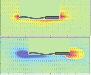
Building upon these results, the flow field around the swimmer at higher  $De$ numbers was resolved. Figure 6 shows a series of time-averaged velocity profiles for Newtonian (figure 6a,c,e) and viscoelastic (figure 6b,d, f) fluids at a fixed rotational frequency of
  $\varOmega = 0.7$ Hz (or equivalently
  $De = 1.05$ in the viscoelastic fluid) and various pitch angles and tail thicknesses. For the swimmer with
  $\psi = 47.5 ^{\circ }$ and
  $d = 2.1\ {\rm mm}$ in the Newtonian fluid (figure 6a), the front–back flow is similar to that of figure 5(a). However, interestingly, for the same conditions in the viscoelastic fluid, we observe a strong front–back flow asymmetry that is characterized by the formation of a negative wake downstream of the swimmer's body (figure 6b). To the best of our knowledge, this is the first report of its kind on the formation of a strong negative wake downstream of a helical swimmer in viscoelastic fluids.

Figure 6. Time-averaged velocity field around a swimmer in the Newtonian fluid (a,c,e) and the viscoelastic fluid (b,d, f). The swimmer pitch angle and tail thickness ( $\psi,{d}$) are (
 $47.5^{\circ }, 2.1\ {\rm mm}$) for (a,b), (
 $12.5^{\circ }, 2.1\ {\rm mm}$) for (c,d) and (
 $47.5^{\circ }, 1.1\ {\rm mm}$) in (e, f).
At a smaller pitch angle ( $\psi = 12.5^{\circ }$), for which
  $U/U_{N}<1$, the same front–back flow asymmetry is observed in the viscoelastic fluid (see figure 6d). Evidently, as the pitch angle decreases, the backward flow downstream of the swimmer's body becomes stronger in the viscoelastic fluid (compare figure 6b with figure 6d). Furthermore, at a smaller tail thickness
  $d = 1.1\ {\rm mm}$ (figure 6e, f), the Newtonian flow around the swimmer does not change appreciably compared with other Newtonian cases shown in figure 6(a,c). However, a direct comparison between flow fields in the viscoelastic fluid (cf. figure 6b, f) reveals that as the tail thickness decreases, the negative wake downstream of the swimmer's body becomes stronger. Sample representative movies used for the above PIV analysis are included as supplementary materials are available at https://doi.org/10.1017/jfm.2022.378.
In summary, our experiments indicate that the viscoelastic flow around the helical swimmer is accompanied by a striking front–back flow asymmetry at high Deborah numbers. This flow asymmetry is characterized by formation of a negative wake in the rear of the swimmer. The strength of the negative wake is inversely proportional to the normalized swimming speed. How can we understand the swimming dynamics and the intertwined effects of swimmer shape and viscoelasticity in the context of this flow asymmetry? To shed more light on the above experimental observations, we performed 3-D numerical simulations of helical swimming in a FENE-P fluid model for conditions that are matched to those of experiments.
3.4. Numerical results
Based on the experimental results of figure 6, the viscoelastic flow around the swimmer is very complex with a strong extensional flow in the wake of the swimmer. Therefore, for simulations we use a FENE-P fluid model, which is known to accurately describe the extensional rheology of viscoelastic fluids (Entov & Hinch Reference Entov and Hinch1997). The simulations are performed using the exact swimmer dimensions, a viscosity ratio  $\beta = 0.9$ and a finite extensibility
  $L^{2}\approx 9$.
Figure 7(a–c) shows averaged steady state flow velocity for three representative cases with different helix pitch angles and thicknesses in the Newtonian and the viscoelastic fluids that correspond to experimental conditions of figure 6. The most substantial changes are observed at the helix region. First, consistent with our experiments, a negative wake downstream of the swimmer's body is observed in simulations of the FENE-P model. Second, increasing the tail thickness at a fixed tail pitch angle, gives rise to a weaker negative wake in simulations (cf. figure 7a,b). Additionally, decreasing the pitch angle at a fixed tail thickness gives rise to a stronger negative wake behind the swimmer (cf. figure 7b,c). These trends are consistent with our experimental observations.

Figure 7. (a–c) The relative mean streamwise velocity of a swimmer in Newtonian and FENE-P viscoelastic fluids with  $\beta =\mu _s/(\mu _s+\mu _p)=0.9$,
  $De=1.05$ for (
 $47.5^{\circ },2.1\ {\rm mm}$) in (a) and (
 $12.5^{\circ },2.1\ {\rm mm}$) in (b) and (
 $47.5^{\circ },1.1\ {\rm mm}$) in (c). (d–f) The mean contribution of the viscoelastic stress tensor in the streamwise direction (
 $\overline {{\partial {\tau _e}_{i1}}/{\partial x_i}}=L_h({1-\beta }/{\beta De})\alpha _p$) of the corresponding (a–c) cases, respectively.
4. Discussion
To better understand the intertwined impacts of swimmer shape, viscoelasticity and front–back flow asymmetry in viscoelastic fluids, we discuss our results using the following approximate force balance. If the flow is approximated as linear Stokes problem, and the viscoelastic stress  $\boldsymbol {\tau }_e$ in (2.1a) is known as an a priori volumetric force from the direct numerical simulation, we can decompose the total axial (streamwise) force on the swimmer into two terms: the first term is the net axial Newtonian force caused by translational motion (with the velocity of
  $U$) and rotation of the helix (with the rotational velocity of
  $\varOmega$), which can be approximated as (Gray & Hancock Reference Gray and Hancock1955)
 \begin{equation} F_{s}= (A_{0}+A_{H}) U -B_{H} \varOmega. \end{equation}
Here  $A_0$ is a positive resistance coefficient and is a function of the size and shape of the swimmer body and the fluid viscosity. The coefficients
  $A_H$ and
  $B_H$ are related to the helix shape and can be approximated using resistive-force theory (Gray & Hancock Reference Gray and Hancock1955) as
 $$\begin{gather} A_{H}\approx (c_{\|} \cos^{2} \psi +c_{{\perp}} \sin^{2} \psi) L_{H}, \end{gather}$$
 $$\begin{gather}B_{H}\approx(c_{{\perp}}-c_{\|})\sin \psi \cos \psi R L_{H}, \end{gather}$$
with  $L_H$ being the length of helix and
  $c_{\perp }=2c_{\|}=4\mu _s {\rm \pi}/\ln (2/\epsilon )$, where
  $\epsilon \ll 1$ is the aspect ratio of the helix.
The second term in the net axial force is caused by the viscoelastic stress tensor in the streamwise direction, and can be written as the volume integral:  $F_e=-\int _V ({\partial {\tau _e}_{i1}}/{\partial x_i})\,{\rm d}V$. At low Reynolds numbers,
  $F_{s}$ and
  $F_{e}$ must balance and the force free-swimming transitional velocity can be expressed as
 \begin{equation} U=\frac{B_{H}}{A_{0}+A_{H}}\varOmega-\frac{1}{A_{0}+A_{H}} F_{e}. \end{equation}
The first term is approximately similar to the Newtonian swimming velocity  $U_N=({B_H}/{A_0+A_H})\varOmega$ (Lauga Reference Lauga2020) and thus, the normalized swimming speed can be written as:
 \begin{equation} \frac{U}{U_{N}}=1+\frac{1}{{B_{H} \varOmega}}\int_V \frac{\partial{\tau_{e}}_{i1}}{\partial x_{i}} {\rm d}V. \end{equation}
 Figure 7(d–f) shows the contour plot of the above volumetric integral for the viscoelastic cases corresponding to figure 7(a–c). While the viscoelastic effects are almost similar near the head and around the swimmer for different cases, there is a substantial difference in the interior of the helix. For the swimmer with  $d=2.1$ mm and
  $\psi =47.5^{\circ }$, the whole region inside the helix is encapsulated by viscoelastic forces that contribute to the thrust. This prediction leads to a swimming speed enhancement, which is consistent with the experimental observations. For other swimmers that correspond to figure 7(a,c), the viscoelastic stresses at the inner region of the helix are predicted to contribute to drag enhancement, which is again consistent with the experimental observations for such cases. Therefore, the above simple force balance argument can explain the swimming dynamics in our experiments based on the contribution of the viscoelastic forces in the region interior to the helix. While
  $De$, and not the helix geometrical characteristics, control the external flow and normal stresses in the outer domain, the helix geometry is the key that can translate those actions into useful forces along the swimming direction. The optimal helix shape is the one that allows the highest acceleration of fluid particles in the inner helix domain and the most constructive use of external hoop stress for improving the swimming speed.
The distribution of viscoelastic stresses around the swimmer's body can generate a pressure distribution on the swimmer's surface. The  $\alpha _p$ parameter noted above encapsulates the combined effects of the viscoelastic stresses and the modified pressure in a volumetric form. To gain a deeper insight into the nature of swimming enhancement or reduction as a result of the change in swimmer's geometry, we have plotted the individual contribution of viscoelastic and pressure forces on the surface of the swimmers. Figure 8 compares the forces from the pressure and viscoelastic stress tensors on the three swimmers noted in figure 7 and their corresponding Newtonian cases. For the swimmer with a small pitch angle (
 $\psi = 12.5^{\circ }$; the top subpanels in figure 8a–c), the viscoelastic stresses do not change the pressure distribution on the swimmer surface compared with the Newtonian fluid. Since the viscoelastic forces generate a net drag on the surface of the helix (evident by a negative
  $\alpha _p$ inside the helix of figure 7e), the swimming speed is expected to be smaller than the Newtonian fluid, which is consistent with the experimental results of figure 3(c).

Figure 8. (a) Viscoelastic stress contribution,  $f_{\tau _e}={\boldsymbol {e}_x^T\boldsymbol {\tau }_e\boldsymbol {n}}/{\rho \varOmega ^2 D^2}$, to the thrust (blue) and drag (red) over the surface of the swimmer in FENE-P fluids. (b) The pressure contribution,
  $f_p=-{\boldsymbol {e}_x^T p \boldsymbol {n}}/{\rho \varOmega ^2 D^2}$, to the thrust (blue) and drag (red) in FENE-P fluids and (c) the pressure contribution to the thrust (blue) and drag (red) in the Newtonian fluid. Here
  $\boldsymbol {e}_x$ is the unit vector in the direction of swimming and
  $\boldsymbol {n}$ is the surface normal. For FENE-P fluid,
  $\beta =\mu _s/(\mu _s+\mu _p)=0.9$ and
  $De=1.05$. Top subpanels are associated with (
 $12.5^{\circ },2.1$ mm), middle subpanels are for (
 $47.5^{\circ },2.1$ mm) and bottom subpanels are for (
 $47.5^{\circ },1.1$ mm).
On the other hand, for the other two swimmers with larger pitch angles shown in middle and bottom subpanels of figure 8(a–c), the reorganization of the viscoelastic stresses on swimmers’ surface significantly changes the pressure distribution compared with the Newtonian counterparts. For the swimmer with larger tail thickness and pitch angle ( $\psi = 47.5^{\circ }, d = 2.1$ mm), the viscoelastic stresses generate a pressure force on the swimmer that is in phase with viscoelastic stresses. Here, the locations where viscoelastic stresses generate thrust (
 $\,f_{\tau e}>0$; e.g. the arrow in figure 8a) coincide with the places where the pressure creates thrust (
 $\,f_p>0$; e.g. the arrow in figure 8b). Therefore, the pressure generated by the viscoelastic forces increases the net thrust of the swimmer's tail (evident with a positive
  $\alpha _p$ in figure 7d), and thereby, enhances the swimming speed beyond the Newtonian fluid. However, for a swimmer with a smaller tail thickness (
 $\psi = 47.5^{\circ }, d = 1.1$ mm), the viscoelastic stresses lead to a pressure distribution along the swimmer tail that is out of phase with the effects of viscoelastic stresses (cf. the dotted arrows in figure 8a,b). This means that produced pressure has a destructive effect on the viscoelastic thrust, and as a result, the overall combined contribution of these effects generates a smaller thrust by the helix (evident by a negative
  $\alpha _p$ parameter in the interior region of the helix in figure 7f).
The above analysis indicates that depending on the swimmer's geometry, the reorganization of the viscoelastic stresses on the swimmer's surface can shift the pressure distribution on the swimmer's body, leading to overall thrust enhancement or reduction. This is similar to previous observations for the viscoelastic flow over cylindrical and infinite helical structures (Phan-Thien & Dou Reference Phan-Thien and Dou1999; Spagnolie et al. Reference Spagnolie, Liu and Powers2013). A full exploration of this effect necessitates substantial computational work to cover all  $De$ and swimmer cases tested in the experiments. In fact, this is the current direction of our research, and it will be discussed in subsequent publications.
Our results suggest that the non-local effects of the viscoelastic stress tensor and the resulting shift in pressure distribution in the helix region play a key role in determining the dynamics of swimming in viscoelastic fluids. The strong rotational shear flow of viscoelastic fluid around the swimmer body gives rise to a hoop stress that develops due to stretching of the polymer molecules along the curved streamlines, and causes a strong extensional flow (or normal stress differences) in the interior region of the helix along the streamwise direction. The extensional flow in the interior of the helix extends to the back of the swimmer and manifests itself as a front–back flow asymmetry accompanied by a strong negative wake downstream of the swimmer's body. However, the results suggest that the front–back flow asymmetry (or the strong negative wake) by itself is not a discriminating metric to rationalize the effects of viscoelasticity on swimming speed. Instead, the progressive engagement of the core flow in the interior region of the helix is the key to better understanding of the impact of viscoelastic forces on swimming dynamics. This mechanism is principally related to local viscoelastic effects near the rotating helix and is inherently distinct from what has been shown theoretically for a ‘snowman swimmer’, a dumbbell composed of two spheres of different diameters (Angeles et al. Reference Angeles, Godínez, Puente-Velazquez, Mendez-Rojano, Lauga and Zenit2021b; Pak et al. Reference Pak, Zhu, Brandt and Lauga2012). In a recent paper, Angeles et al. (Reference Angeles, Godínez, Puente-Velazquez, Mendez-Rojano, Lauga and Zenit2021a) showed that the swimming dynamics of helical swimmers in viscoelastic fluids depend strongly on the front–back geometrical asymmetry; i.e. the difference between the head and the helix diameter. The effects of front–back geometrical asymmetry were explained in the context of snowman-like effects (i.e. effects due to asymmetry between the diameter of the head and the tail of the swimmer) (Angeles et al. Reference Angeles, Godínez, Puente-Velazquez, Mendez-Rojano, Lauga and Zenit2021a). In our paper, the diameters of the head and helix are the same, and therefore snowman-like effects should be minimal. Instead, we think that the contribution of the normal stresses inside the helix and the resulting pressure distributions are the key parameters in the enhancement or diminution of the swimming speed. These stresses are strongly controlled by the properties of the polymer solution and the finite extensibility of the polymer chains.
5. Conclusion
In summary, we have demonstrated that increasing the tail pitch angle and/or the tail thickness of a helical swimmer gives rise to a swimming speed enhancement in a viscoelastic fluid. More importantly, we presented the first evidence for formation of a front–back flow asymmetry around a swimmer, which is characterized by formation of a negative wake downstream of the helical swimmer in the viscoelastic fluid. Our simulations predict a similar front–back flow asymmetry observed in experiments. Furthermore, using a simple force balance argument, we showed that the contribution of the viscoelastic forces in the interior region of the helix are key in controlling the swimming dynamics. These streamwise viscoelastic forces are generated by the hoop stress and are at the origin of the front–back flow asymmetry (or the negative wake downstream of the swimmer's body) in experiments. Despite the negative wake being a signature of swimming in viscoelastic fluids, it is not directly correlated with the enhancement or reduction of swimming speed. Instead, the viscoelastic stresses and the resulting shift in pressure distribution around the swimmer surface are recognized as the key features that contribute to swimming dynamics in the viscoelastic fluid.
Finally, in the current study the helix is actuated via an external torque, while swimming of flagellated bacteria is torque-free and the bacteria body always rotates in the opposite direction to the rotating helix (Lauga Reference Lauga2020). Recent studies have started addressing this problem by devising torque-free robots that could mimic the microorganisms’ swimming strategies (Binagia & Shaqfeh Reference Binagia and Shaqfeh2021; Das et al. Reference Das, Styslinger, Harris and Zenit2021; Kroo et al. Reference Kroo, Binagia, Eckman, Prakash and Shaqfeh2021). Further research is required to address how the swimming performance is affected by these effects, namely the torque-free swimming and the counter rotations of the helix and the cell body in viscoelastic fluids.
Supplementary movies
Supplementary movies are available at https://doi.org/10.1017/jfm.2022.378.
Funding
The authors acknowledge the Florida State University Research Computing Center for the computational resources on which these simulations were carried out and Florida State University Council for Research and Creativity for partially supporting this work.
Declaration of interests
The authors report no conflict of interest.


