
1. Introduction
Despite the very large number of studies on flow-induced vibrations (FIV), none of them considered the case of horizontal wakes in a stratified fluid. This work aims to characterize the influence of a continuous stratification on wake-induced vibrations of a circular cylinder.
Many works have concerned simple geometries such as a circular cylinder that exhibit a large variety of regimes and wake structures. They were initially motivated by applications such as marine cables (Griffin Reference Griffin1985), or taut wires in air (Strouhal Reference Strouhal1878). In this civil engineering context, it is important to minimize or control any undesired vibrations that could damage the structure. For other applications, one could instead be interested in increasing the oscillations as they could be a source of energy when coupled to piezoelectric devices (Bernitsas et al. Reference Bernitsas, Raghavan, Ben-Simon and Garcia2008; Grouthier et al. Reference Grouthier, Michelin, Bourguet, Modarres-Sadeghi and De Langre2014; Song et al. Reference Song, Shan, Lv and Xie2015).
As now documented in textbooks (Tritton Reference Tritton2012) and review articles (Williamson Reference Williamson1996b), the wake of a cylinder is known to exhibit different regimes as the Reynolds number is varied. As the Reynolds number increases, one observes successively the breaking of the upstream/downstream symmetry, the appearance of a separation bubble (Coutanceau & Bouard Reference Coutanceau and Bouard1977), vortex shedding (Von Karman Reference Von Karman1911) and a series of three-dimensional transitions (Williamson Reference Williamson1996a). One of the most remarkable features is the persistence of the von Kármán vortex street for Reynolds numbers as large as  $10^7$ (Roshko Reference Roshko1961). These coherent structures induce coherent pressure fluctuations on the cylinder that are responsible for lift and drag fluctuations. When the cylinder is free to move, this induces transverse oscillations (Feng Reference Feng1968), so-called vortex-induced vibrations (VIV). Reviews can be found in Bearman (Reference Bearman1984), Williamson & Govardhan (Reference Williamson and Govardhan2004) and Sarpkaya (Reference Sarpkaya2004).
VIV have generally been studied experimentally by mounting a circular cylinder on springs in a water channel or a wind tunnel. The system then possesses two reference frequencies:
(i) The frequency
 $f_n$ associated with the transverse displacement of the structure given by the natural frequency of the springs
(1.1)where\begin{equation} 2 {\rm \pi}f_n=\sqrt{\frac{k}{(m+m_A)}} , \end{equation}$k$ is the spring constant, $m$ the cylinder mass and $m_A$ the potential added mass.
$f_n$ associated with the transverse displacement of the structure given by the natural frequency of the springs
(1.1)where\begin{equation} 2 {\rm \pi}f_n=\sqrt{\frac{k}{(m+m_A)}} , \end{equation}$k$ is the spring constant, $m$ the cylinder mass and $m_A$ the potential added mass.(ii) The frequency
$f_V$ associated with vortex shedding given for a fixed cylinder by an empirical formula
(1.2)where\begin{equation} f_V=St \frac{U}{D} , \end{equation}$St$ is the Strouhal number (Strouhal Reference Strouhal1878), $U$ the fluid velocity and $D$ the cylinder diameter. The value of $St$ is found experimentally to be close to $0.2$ in a large range of Reynolds numbers $200< Re <200\,000$ (Lienhard Reference Lienhard1966).


In the classical VIV theory (reviewed by Williamson & Govardhan (Reference Williamson and Govardhan2004), for instance) the vortex-shedding frequency is found to synchronize with  $f_n$ when
  $f_V$ reaches
  $f_n$ (Den Hartog Reference Den Hartog1954). Both the structure oscillations and vortex shedding then remain locked in at almost a constant frequency in a large interval of velocities. For large mass ratio
  $m^*$ (equal to the cylinder mass
  $m$ divided by the mass of an equivalent volume of fluid), this frequency is close to
  $f_n$, as observed in the experiments in air performed by Feng (Reference Feng1968) where
  $m^*=248$. For small
  $m^*$ below 20 (Khalak & Williamson Reference Khalak and Williamson1996, Reference Khalak and Williamson1997, Reference Khalak and Williamson1999), this mode of constant lock-in frequency is again observed, called the ‘lower branch mode’, but with higher amplitudes and a larger frequency compared to high mass ratio experiments. This lock-in frequency non-dimensionalized by
  $f_n$ has been determined empirically by Govardhan & Williamson (Reference Govardhan and Williamson2000) for a circular cylinder as
 \begin{equation} f^{*}_{{lower}}=\sqrt{\frac{m^*+C_A}{m^*-0.54}}, \end{equation}
where the added mass coefficient  $C_A$ is set to 1. Furthermore, in this low
  $m^*$ case, a second ‘upper branch mode’ is observed. It results in oscillations of even larger amplitude than the first mode. The oscillations start when
  $f_V$ reaches
  $f_n$, and have a frequency which grows with the velocity up to
  $f^{*}_{{lower}}$, where the system switch to the lower branch mode.
Another type of FIV can also come from the breaking of the axisymmetry of the object, it is called galloping. When the object is not circular, a small angle of incidence may induce a destabilizing lift force. This leads to high-amplitude low-frequency oscillations that have been studied for rectangular cylinders (Mannini, Marra & Bartoli Reference Mannini, Marra and Bartoli2014), and modified circular cylinder geometries (Nakamura, Hirata & Kashima Reference Nakamura, Hirata and Kashima1994; Chang, Kumar & Bernitsas Reference Chang, Kumar and Bernitsas2011). Some studies have also considered the interaction of galloping and vortex shedding (Parkinson & Wawzonek Reference Parkinson and Wawzonek1981; Mannini et al. Reference Mannini, Marra, Massai and Bartoli2016). Note finally that there exist other FIV phenomena such as buffeting (Blevins Reference Blevins1977), or resulting from the interaction of several objects (Assi, Bearman & Meneghini Reference Assi, Bearman and Meneghini2010).
Studies of transverse FIV have considered very complex systems but surprisingly have never tried to include stratification, while most fluids in the environment are stratified. A stably stratified fluid has a density that increases with depth. An important consequence of this is that vertical displacements of fluid parcels are inhibited in stratified flows. Indeed, each fluid parcel is at equilibrium at its initial vertical position and experiences a restoring force if displaced vertically. Following Tritton (Reference Tritton2012), let us consider a fluid particle of density  $\rho (0)$ that is vertically displaced of a distance
  $\Delta z$. If the adiabatic temperature gradient is negligible, the density of the new surrounding fluid is
 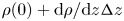 $\rho (0) + \textrm {d}\rho /\textrm {d}z {\rm \Delta} z$. Then, with the joint association of weight and buoyancy forces, the particle motion is governed by equation
 \begin{equation} \rho(0) \frac{\textrm{d}^2 \Delta z}{\textrm{d}t^2} = g \frac{\textrm{d} \rho}{\textrm{d}z} \Delta z, \end{equation}
where  $\boldsymbol {g}$ is the gravity along the vertical direction
  $\boldsymbol {z}$. In a stably stratified fluid, as considered here, the density gradient is negative. This equation then indicates that the particle oscillates around its initial position at the so-called Brünt–Väisälä frequency,
  $N$, defined by
 \begin{equation} N^2 ={-}\frac{g}{\rho(0)}\frac{\partial\rho}{\partial z} . \end{equation}
This new additional frequency in the system is expected to influence the VIV phenomena described above.
Stratification is already known to modify the wake of a fixed cylinder. As it inhibits vertical motion, it delays the appearance of vortex shedding and narrows the vertical extent of the wake (e.g. Lin & Pao Reference Lin and Pao1979; Honji Reference Honji1988). It can also be responsible for the appearance of a second vortex-shedding mode when the cylinder is tilted with respect to the horizontal plane (Meunier Reference Meunier2012).
The reference experimental study describing the wake of a horizontal circular cylinder has been carried out by Boyer et al. (Reference Boyer, Davies, Fernando and Zhang1989). They have observed 10 different types of regimes as the Reynolds number and the stratification strength are varied. Even more regimes have been found in Chashechkin & Voyekov (Reference Chashechkin and Voyekov1993). Further quantitative studies have been performed since then. Ohya, Uchida & Nagai (Reference Ohya, Uchida and Nagai2013) measured Strouhal numbers on various cylinder diameters in wind tunnel experiments with large Reynolds numbers (between 3500 and 12 000). They showed a drastic change of the wake pattern strongly influencing the Strouhal number at a Froude number close to  $Fr=U/ND=2$. Numerically, at low Reynolds numbers, Hwang & Lin (Reference Hwang and Lin1992) predicted the lift and drag coefficients.
In the present work, we start exploring experimentally the new field of ‘stratified wake-induced vibrations’ for the simple and most documented geometry of a circular cylinder in a large Reynolds number regime. The objective is to evidence some new phenomena, describe their characteristics and tentatively provide some physical explanations.
The paper is organized as follows. In § 2, the experimental set-up is first described. The main control parameters of the problem are identified. Reference data with a fixed cylinder are also obtained. In § 3, the FIV results are presented. Two oscillation modes are obtained which are successively discussed in §§ 4 and 5. In § 5, some numerical computations are also performed to identify the mechanism of instability. In § 6, the competition between the two modes is further studied, to propose a stability diagram for the system. A brief conclusion is made in § 7.
2. A stratified VIV experiment
2.1. Facility
The experimental set-up, sketched in figure 1, consists of a polymethyl methacrylate (PMMA) tank 4 m long, 1 m wide and 1 m deep, which is filled with salty water up to a height  $H$ between 70 and 85 cm. A trolley is mounted on rails and moved with a ball screw connected to a motor MAC800 D2 of JVL, allowing a horizontal translation of the system along the tank. The velocity of the trolley is kept constant during each run and varies in the range
  $1.3 \leqslant U \leqslant 23\ \textrm {cm}\ \textrm {s}^{-1}$.

Figure 1. Sketch of the experimental set-up with the main parameters: velocity  $U$, length of arms
  $L$, cylinder diameter
  $D$ and the Brünt–Väisälä frequency
  $N$ defined by (1.5).
Three different cylinders of diameter  $D$ (equal to 3.2, 4 and 6.2 cm) and length
  $L_y$ of 63.9 cm are considered. This leads to large ratios
  $L_y/D>10$ and
  $H/D>12$ which minimizes end effects in the transverse direction
  $y$ and at the top and bottom of the tank.
As illustrated in figure 1, the cylinder is mounted on flat blade-shaped arms, which are free to rotate around their junction point with the supports thanks to ball bearings. The length  $L$ of these arms is an important parameter chosen between 15 and 50 cm.
Using a similar set-up in a homogeneous fluid, De Wilde, Huijsmans & Triantafyllou (Reference De Wilde, Huijsmans and Triantafyllou2003) considered two spring blade lengths, with an equivalent ratio  $L/D$ of 12 and 24. They concluded that the in-line motion of the cylinder and its small rotation did not influence the VIV for oscillation amplitudes below 0.6
 $D$, which are the larger ‘VIV’ amplitudes we obtain in the present study (see § 4). Even though in our experiments the
  $L/D$ value can be as low as 2.42, the results did collapse whatever the aspect ratio, which indicates that these effects remain small.
The flat shape of the arms and of their junction with the cylinder, using two screws, limit tilting and minimize the arm-induced drag. Indeed, an estimation of this drag compared to the cylinder drag can be obtained in homogeneous water using the formula for a thin flat plate inclined of an angle  $\theta$ to the flow, given by Blevins (Reference Blevins1984). It shows that, for the angles obtained here (
 $14^{\circ }$ at most), and in the ‘worst’ configuration (i.e. with longer arms and smaller cylinder), both arms induce only approximately 4 % of the cylinder drag. This justifies that arm drag will be neglected in the following. All the parameters of every experiment performed are summarized in table 1.
Table 1. Parameters of the different experimental configurations. For each configuration, approximately 20 different values of the translation velocity are considered between  $1.3$ and
  $23\ \textrm {cm}\ \textrm {s}^{-1}$. The last column indicates the symbol used for each experiment in the figures.

The damping induced by ball bearings is measured in air using the pendulum model
 \begin{equation} \ddot{\theta}+\frac{c}{m}\dot{\theta}+\omega_0^2\theta = 0, \end{equation}
with  $\omega _0=\sqrt {g/L} \approx 4.43\ \textrm {rad}\ \textrm {s}^{-1}$ for arms of length
  $L=50$ cm. The damping coefficient
  $c$ is found by fitting the exponential decay of the cylinder position over 96 periods, and found to be
  $c=5.6 \pm 0.2 \times 10^{-3}\ \textrm {kg}\ \textrm {s}^{-1}$ (for a cylinder of mass
  $m=525 \pm 0.1\ \textrm {g}$ in this experiment). It corresponds to a damping ratio
  $\zeta =c/2m\omega _0=1.20 \pm 0.05 \times 10^{-3}$.
The mass  $m$ of the cylinder is adjusted within 1 % so that it is at equilibrium when the arms are roughly horizontal. This was done by adding (respectively removing) mass from inside the hollow cylinder, and by using steel (respectively plastic) screws. The uncertainties are such that, at rest, the cylinder is at
  $50 \pm 4\ \textrm {cm}$ from the bottom of the tank.
2.2. Stratification
The tank is filled with salty water with a salt concentration increasing linearly with depth. The fluid density can be written as  $\rho =\rho _0(1-zN^2/g)$, where
  $\rho _0$ is the density at the cylinder equilibrium position.
This stratification is obtained using a technique described in Bosco (Reference Bosco2015). It consists of dividing the tank into two parts, one with pure water and the other one with uniformly mixed strongly salty water, and letting the two fluids mix through holes of diameter 0.5 cm drilled in the separation slab. This technique is preferred to the usual ‘two tanks method’ because it requires only one tank, which is far more convenient considering the huge volume used here.
A plot of the density profile just after the stratification creation is shown in figure 2. One can notice that the profile is linear from  $z=20\ \textrm {cm}$ to the free surface at
  $z=85\ \textrm {cm}$, but a mixed layer is observed for
  $z< 20\ \textrm {cm}$. This is due to a stronger mixing occurring at the bottom when the salty and pure water blend through the slab holes. We have been able to limit this effect that could also happen at the free surface by closing some of the holes.

Figure 2. Plot of the density profile two days after the creation of the stratification. By taking  $\rho _0=\rho \ (z=50\ \textrm {cm})=1.046\ \textrm {g}\ \textrm {cm}^{-3}$ as density reference, one can find
  $N=1.06\ \textrm {rad}\ \textrm {s}^{-1}$.
Experiments are typically performed during a few months with the same water. During this period, the value of  $N$ decreases progressively owing to leaks and the mixing generated by the displacements of the cylinder. In order to minimize these effects, the tank is regularly filled with fresh water at the top and/or salty water at the bottom. Every experimental day, a density profile is measured to recompute
  $N$, but mixing still induces uncertainties on
  $N$ from 2 % up to 25 % for the runs with the largest cylinder diameter and the strongest oscillations.
2.3. Important non-dimensional parameters
From the geometrical parameters ( $D, L, H, L_y$), as defined in figure 1, the translation speed
  $U$ and the fluid properties (kinetic viscosity
  $\nu$, diffusion coefficient
  $\mathcal {D}$ and
  $N$), an important number of non-dimensional parameters can be defined:
(i) the Reynolds number
$Re = UD/\nu$;(ii) the Froude number
$Fr = U/ND$;(iii) the length ratio
$l = L/D$;(iv) the Schmidt number
$Sc = \nu /\mathcal {D}$;(v) the mass ratio
$m^* = m/(\rho _0 L_y {\rm \pi}D^2/4)$;(vi) the geometric ratios
$L_y/D$ and $H/D$.


The last two ratios are large. For this reason, end effects as well as boundary effects associated with the free surface, side and bottom walls are assumed to be negligible. They are not considered in the present study. The Schmidt number is close to  $Sc\approx 625$ obtained for
  $\nu = 10^{-6}\ \textrm {m}^2\ \textrm {s}^{-1}$ and
  $\mathcal {D} =1.64\times 10^{-9}\ \textrm {m}^2\ \textrm {s}^{-1}$. The mass ratio
  $m^*$, is here always equal to 1, which is considered as a very low mass ratio in usual VIV experiments (Khalak & Williamson Reference Khalak and Williamson1997, Reference Khalak and Williamson1999).
In the present study, the three important parameters are then  $Re$,
$Re$,  $Fr$ and
  $l$. They will be varied in the following ranges:
  $500 < Re < 15\,000$;
  $0.5 < Fr < 19$;
  $2 < l < 16$. Of interest is also the ratio
  $Re /Fr$ that remains constant for each experiment number indicated in table 1. Except for the non-stratified case (experiment number 7), this ratio is large, indicating the dominance of buoyancy over viscous effects.
2.4. Measurements with fixed cylinder: the Strouhal number
The Strouhal number, defined in (1.2), corresponds to the non-dimensional frequency associated with vortex shedding for a fixed cylinder. There are only a few data for the Strouhal number law in a stratified fluid. For this reason, experiments with a fixed cylinder are first performed in order to find the Strouhal number dependence in the set-up.
Three different cylinders of diameter  $D=2.1$, 3.1 and 4.1 cm are considered. The measurements were made by analysing the wake patterns in the last two metres of the cylinder course with a shadowgraph method using a camera Sony
  $\alpha 7s$ taking 25 frames per second, and lens FE 2.8/50 MACRO. This visualization technique reveals regions of the flow where the second derivative of the density field with respect to the isopycnal's normal is positive or negative.
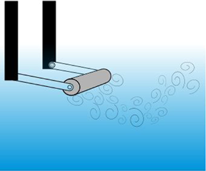
Observed patterns are qualitatively described in Boyer et al. (Reference Boyer, Davies, Fernando and Zhang1989), who compiled 10 different regimes in the  $Fr\text {--}Re$ plane. Figure 3 shows a comparison between their results and the present study. A wave regime is present at low Froude numbers, as the stratification is strong (denoted as single and multiple centreline structures by Boyer et al. Reference Boyer, Davies, Fernando and Zhang1989). Lee waves develop behind the cylinder, due to the oscillatory motion of fluid parcels initially forced to move in the vertical direction by the cylinder passing. The existence of a blocking region ahead of the cylinder can also be observed. It is typical of strongly stratified fluids: see for example Graebel (Reference Graebel1969) for the theory, Browand & Winant (Reference Browand and Winant1972) for the first experiments, the book of Tritton (Reference Tritton2012) or the review of Lin & Pao (Reference Lin and Pao1979) for a comprehensive description of the phenomenon. With increasing
  $Fr$, the flow starts to separate behind the cylinder and eddies develop. The quite remarkable regime of isolated mixed regions is characterized by a first wake narrowing after the recirculation zone, followed by a localized expansion around a closed mixed region. It is also interesting to note that Boyer et al. (Reference Boyer, Davies, Fernando and Zhang1989) showed that this mixed region is dynamic: its streamwise location as well as its thickness depend on time, and oscillate. The last wake pattern presented here looks like a usual turbulent vortex-shedding state. In this so-called turbulent vortical structure regime, the stratification is too weak to prevent the formation of vortices, but it tends to delay their formation and reduce the wake expansion (especially visible on Boyer's picture).

Figure 3. Wake patterns observed by shadowgraph compared to those presented by Boyer et al. (Reference Boyer, Davies, Fernando and Zhang1989). For more precision about the regimes and their relative position in the  $Fr\text {--}Re$ plane, see Boyer et al. (Reference Boyer, Davies, Fernando and Zhang1989).
The frequency was measured and dimensionalized to obtain the Strouhal number. Results are plotted in figure 4 as a function of the Froude number, which offers the best collapse.

Figure 4. Strouhal number as a function of the Froude number.  $D=2.1\ \textrm {cm}$ (green),
  $D=3.1\ \textrm {cm}$ (blue) and
  $D=4.1\ \textrm {cm}$ (red). Black symbols stand for experimental (stars) and numerical (dots) results of Meunier (Reference Meunier2012) (
 $Re \in [40,200]$).
The Reynolds number is equal to  $Re = 410 \, Fr$ for
  $D=2.1$ cm, to
  $Re = 894\,Fr$ for
  $D=3.1$ cm, to
  $Re =1563\,Fr$ for
  $D=4.1$ cm. The Reynolds number ranges from 400 to 8000 in these experiments. On this plot is also displayed the experimental and numerical results obtained by Meunier (Reference Meunier2012) for lower Reynolds numbers (
 $40 < Re < 200$). This figure clearly shows that the usual value
  $St\approx 0.2$ of the homogeneous case remains valid here as soon as
  $Fr >1.5$.
For lower  $Fr$, a sudden increase of the vortex-shedding frequency is observed, in agreement with the numerical and experimental results of Meunier (Reference Meunier2012) and Ohya et al. (Reference Ohya, Uchida and Nagai2013). We can also see that this increase becomes larger when the diameter of the cylinder is increased for a fixed
  $Fr$. This means a growth of the Strouhal number with the Reynolds number for small fixed
  $Fr$. This tendency is in agreement with the results obtained by Chashechkin & Voyekov (Reference Chashechkin and Voyekov1993) who observe a linear increase of
  $St$ with
  $Re$ for small Froude numbers.
2.5. Measurements with oscillating cylinder and sources of uncertainty
As for the fixed cylinder, FIV measurements were performed in the last two metres of the cylinder course with the same apparatus. This means that, when entering the record area, the cylinder was already towed on approximately two metres. Oscillations then started to settle (this can be seen in figure 5 for example).

Figure 5. Vertical position of the cylinder in a homogeneous flow (green) and in a weakly stratified flow with  $N=0.37\pm 0.02\ \textrm {rad}\ \textrm {s}^{-1}$,
  $Fr=6.16$ (red). Measurements are for experiment numbers 7 and 4 of table 1, at
  $Re=4158$.
The software Tracker, a video analysis tool, is capable of following the positions of the ball bearing and of the cylinder. To do so, the user needs to manually target the interesting point on the first image and define a surrounding zone. The software compares the surrounding zone pixel pattern with reduced areas of the next image, to find the best correlation. This method is accurate up to a few pixels (video quality is the main limitation). It induces an error of the order of a millimetre, negligible in this study. The oscillations of the cylinder are then deduced from the calculated angle  $\theta$ made by the cylinder–ball bearing line with respect to the horizontal. Amplitude
  $A$ and frequency
  $f$ are obtained from a least squares fit of the time variation of the angle.
Sources of uncertainties coming from the visualization method or the stratification measurement for instance, are numerous. A few of them can be quantified.
Uncertainties on the Froude number  $Fr$ come from the variation of
  $N$ due to mixing. As already mentioned (§ 2.2), they are mostly lower than
  $7\,\%$ although they can reach
  $20\,\%$ to
  $25\,\%$, like in experiments 1 and 8 (see table 1).
Uncertainties on the Reynolds number  $Re$ of approximately
  $10\,\%$ are mainly due to temperature variation, which modifies the value of the kinematic viscosity.
Uncertainties on the oscillation frequency and amplitude measurement are of order  $10$ and
  $15\,\%$ for the higher-frequency mode (see § 4), mainly due to the limited number of observed oscillations. For the low-frequency mode, they are of order
  $5\,\%$ (up to
  $10\,\%$ for frequency and to
  $15\,\%$ for amplitude measurements in low-amplitude experiments).
The overall uncertainty present in the measurements is well represented by the scatter in the figures. Although this scatter is important, it is much smaller than the variation of the amplitude and of the frequencies by a factor of approximately 10 in the range considered in this paper. These quantitative data are thus sufficient to draw convincing conclusions.
3. Effects of stratification
3.1. Comparison to homogeneous fluid
Videos of the cylinder moving through the tank were analysed to deduce the evolution of vertical position  $z$ of the cylinder as a function of time. A plot of these raw data, in a homogeneous and a stratified fluid, for fixed
  $l$ and
  $Re$, is shown in figure 5. Note that the initial time
  $t=0s$, corresponds to the time at which the cylinder enters the camera's field of view. For this reason, the cylinder is not necessarily at the reference position
  $z=0$ at
  $t=0$.
Figure 5 shows clearly that the cylinder exhibits strong oscillations in a stratified fluid whereas the oscillations are almost undetectable in a homogeneous fluid. This is a first indication that stratification strongly affects the flow-induced vibrations of a cylinder.
Measurements of the amplitude and frequency of the cylinder oscillations are reported in figure 6 as a function of the Reynolds number for the homogeneous and stratified cases. It confirms that, although oscillations are observed in both cases, their amplitudes in stratified water are more than one decade higher than in a homogeneous fluid. Their frequencies non-dimensionalized by  $U/D$ are approximatively constant but they are larger in the homogeneous case.

Figure 6. Amplitude (a) and frequency (b) of the cylinder oscillations as a function of the Reynolds number in a stratified (red) and homogeneous (green) fluid for experiment numbers 7 and 4. In the stratified case,  $N=0.37\pm 0.02\ \textrm {rad}\ \textrm {s}^{-1}$ and
  $Fr$ varies from 1.8 for the smaller Reynolds number, to 12.6 for the larger one.
3.2. The existence of two vibration modes
The stratified experiments were repeated with different speeds  $U$, cylinder diameters
  $D$ and arm lengths
  $L$ to explore the space of the parameters
  $Fr$,
$Fr$,  $Re$ and
  $l$.
$l$.
Data of measured amplitudes  $A$ and frequencies
  $f$ obtained for a fixed value of
  $l$ are shown in figure 7. The uncertainty in the measurements is here mainly due to
  $N$. Note that the error bars are smaller than the scatter in the data. They will not be shown in the following figures since the scatter is sufficient to represent this uncertainty.

Figure 7. Amplitude (a) and frequency (b) of the cylinder oscillations with error bars as a function of the Froude number for one set of cylinder diameter and length of arms (Experiment number 12,  $N=1.07\pm 0.15\ \textrm {rad}\ \textrm {s}^{-1}$, for further information see table 1).
Figure 7 shows that, as  $Fr$ increases, the cylinder firstly exhibits large-amplitude vibrations at low frequency (with an amplitude peak around
  $Fr=1.5$). Then, the oscillations almost disappear before increasing again, to a lesser extent, while their frequency jumps to a value about six times their initial one. This indicates the existence of two distinct vibration modes.
These two modes are also clearly visible in figure 8, where we plot the measured frequencies and amplitudes for all studied  $l$ as a function of
  $Fr$.
$Fr$.

Figure 8. Amplitude (a) and frequency (b) of the cylinder oscillations as a function of the Froude number for all  $l$ considered. Black, red and blue symbols stand for the larger, intermediate and smallest cylinder diameters, respectively (see table 1). Only experiments with amplitude oscillations larger than
  $0.03D$ are plotted.
For visibility reasons, only measurements for which the oscillation amplitude was larger than  $0.03D$ are kept in the frequency graph. This amplitude threshold has also been applied to all the following frequency plots, except the final ones of § 6.
The large amount of data extending from low  $Fr$, less than one, up to
  $Fr \sim 16$ enables us to better identify the two frequency modes already spotted on figure 7. The first mode has a low frequency of order
  $0.25N/2{\rm \pi}$. It is obtained for small Froude numbers between 1 and 3 and is favoured by large
  $l$. The second mode has a higher frequency that increases with
  $U$.
$U$.
Concerning the amplitudes of the modes, the first one has an amplitude as large as  $2D$. It corresponds to the peak observed for low Froude numbers in figure 8(a). The second mode exhibits non-negligible amplitudes up to
  $0.6D$ for larger Froude numbers. The amplitude graph shows a strong scatter in the data, especially at intermediate Froude numbers between 2 and 6, where the system seems to switch from one mode to the other.
In the next two sections, a focus is made on each frequency branch to detail the observations and provide some physical interpretations.
4. The VIV analogous mode
The high-frequency mode is firstly considered. The objective is to show that it can be understood thanks to the models developed in classical VIV theory. For this purpose, a simple mathematical model is derived to estimate the natural frequency  $f_n$ of the mechanical system.
The model is based on the application of the momentum equation to the cylinder assuming that the forces acting on the rod can be neglected (small mass, negligible drag). For a cylinder of density  $\rho _{s}$, volume
  $V_s$, diameter
  $D$ and length
  $L_y$, supported by a rigid rod of length
  $L$ which makes an angle
  $\theta$ with respect to the horizontal plane (see figure 9), the following forces acting on the cylinder can be listed:
(i) Rod's tightness
$\boldsymbol {F}_{\boldsymbol {T}}$.(ii) Weight
$\boldsymbol {F}_{\boldsymbol {w}}=\rho _{\boldsymbol {s}}V_{s}\boldsymbol {g}$.(iii) Buoyancy force
$\boldsymbol {F}_{\boldsymbol {b}}=-\rho (\theta )V_{s}\boldsymbol {g}$.(iv) Drag force
$\boldsymbol {F}_{\boldsymbol {D}}=-\frac {1}{2}\rho (\theta )DL_yC_{D}U_{abs} \boldsymbol {U}_{\boldsymbol {abs}}$.(v) Lift force
$\boldsymbol {F}_{\boldsymbol {L}}=-\frac {1}{2} \rho (\theta )DL_yC_{L}U_{abs}(\boldsymbol {e}_{\boldsymbol {y}} \wedge \boldsymbol {U}_{\boldsymbol {abs}})$.(vi) Added mass force
$\boldsymbol {F}_{\boldsymbol {a}}=-C_A\rho (\theta )V_{s}L(\ddot {\theta }\boldsymbol {e}_{\boldsymbol {\theta }}- \dot {\theta }^2\boldsymbol {e}_{\boldsymbol {r}})$.(vii) Ball bearing damping
$\boldsymbol {F}_{\boldsymbol {d}}=-cL\dot {\theta }\boldsymbol {e}_{{\boldsymbol {\theta }}}$.


Figure 9. Schematic of the problem. Opposite or perpendicular forces are coloured by pair to ease comprehension.
Here,  $C_D$ and
  $C_L$ denote the drag and lift coefficients, respectively,
  $C_A$ the added mass coefficient for a circular cylinder and
 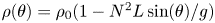 $\rho (\theta ) = \rho _0(1-N^2L\sin (\theta )/g)$ the density of the ambient fluid at the cylinder position. Assuming the cylinder at rest when
  $\theta =0$, one has
  $\rho _s=\rho _0$. Figure 9 shows these forces and their orientations. The absolute velocity
  $\boldsymbol {U}_{\boldsymbol {abs}}$ is the effective velocity of the cylinder due to the combined action of its translation by the trolley and its rotation around the ball bearing caused by oscillations, so that
 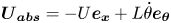 $\boldsymbol {U}_{\boldsymbol {abs}}=-U\boldsymbol {e}_{{\boldsymbol {x}}}+L \dot {\theta }\boldsymbol {e}_{{\boldsymbol {\theta }}}$. By definition, the drag force is oriented in the direction of
  $-\boldsymbol {U}_{\boldsymbol {abs}}$ while the lift force is perpendicular to it.
The drag coefficient  $C_D$ is considered constant and equal to 1, which is the value for a static cylinder and for Reynolds numbers between
  $10^3$ and
  $10^4$ (von Wieselsberger Reference von Wieselsberger1921; Blevins Reference Blevins1984). The drag coefficient varies when the cylinder oscillates (Khalak & Williamson Reference Khalak and Williamson1996, Reference Khalak and Williamson1999) but its mean value is found to remain not far from 1, as observed experimentally (Bishop & Hassan Reference Bishop and Hassan1964; Yamamoto & Nath Reference Yamamoto and Nath1976; Bearman et al. Reference Bearman, Downie, Graham and Obasaju1985), and numerically for low Reynolds numbers (Guilmineau & Queutey Reference Guilmineau and Queutey2002; Zheng & Zhang Reference Zheng and Zhang2008; Placzek, Sigrist & Hamdouni Reference Placzek, Sigrist and Hamdouni2009). Sarpkaya (Reference Sarpkaya1978) proposed the law
 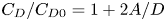 $C_D/C_{D0}=1+2A/D$ where
  $C_{D0}$ denotes the drag value for a fixed cylinder. This formula seems to be confirmed by Khalak & Williamson (Reference Khalak and Williamson1999), especially for low mass ratios. The present VIV-like mode amplitudes mainly lie between 0.1D and 0.6
 $D$, so this effect may double the value of
  $C_D$ for the largest amplitudes. As will be shown, this induces a change lower than 40 % of the predicted frequency, which is smaller than the uncertainties and the scatter in the data. For this reason, we have neglected this effect and chosen a fixed and constant value
  $C_D=1$ for the present study.
Applying the operation  $\boldsymbol {e}_{\boldsymbol {r}} \times$ to the momentum equation leads to the angular momentum equation
 \begin{align} V_{s}(\rho_0+\rho C_A)L\ddot{\theta}+cL\dot{\theta} = \frac{F_D}{U_{abs}}[U\sin(\theta)+L\dot{\theta}]-\frac{F_L}{U_{abs}} U\cos(\theta)+(\rho_0-\rho)V_{s}g\cos(\theta). \end{align}
 By assuming  $\theta \ll 1$ (in light of experimental observations),
  $C_A=1$, keeping only the first-order terms, and switching from
  $\theta$ to
  $z=L\theta$, the following equation is obtained:
 \begin{equation} \ddot{z}+\left(\frac{c}{2\rho_0V_{s}}+\frac{C_D U}{{\rm \pi} D}\right)\dot{z}+\left(\frac{N^2}{2}+\frac{C_D U^2}{{\rm \pi} LD}\right)z = \frac{C_LU^2}{{\rm \pi} D}. \end{equation}
This is the classical equation of a forced damped oscillator, that is forced by the fluctuating lift and damped by ball bearings and drag force.
Equation (4.2) shows that the restoring forces due to drag and stratification combine to create an oscillator of natural frequency
 \begin{equation} f_{n} = \frac{1}{2 {\rm \pi}}\sqrt{\frac{N^2}{2}+\frac{C_DU^2}{{\rm \pi} LD}} . \end{equation}
This formula applies to both homogeneous and stratified cases.
In the absence of stratification, the natural frequency is
 \begin{equation} f_{n0}=(U/2 {\rm \pi}D) \sqrt{C_D/{\rm \pi} l}. \end{equation}
The non-dimensional velocity
 \begin{equation} U^* = \frac{U}{f_nD} \end{equation}
that is commonly used in VIV studies (Williamson & Govardhan Reference Williamson and Govardhan2004), is thus constant and equal to
 \begin{equation} U_0^*=2{\rm \pi}^{3/2}\sqrt{l/C_D}. \end{equation}
 In experiment number 7 (table 1), one can calculate  $U_0^* \approx 21.5$. This value is very large compared to the value
  $1/St = 5$ where high-amplitude VIV oscillations are expected in the classical theory (see § 1). In other words, the natural mechanical frequency and the vortex-shedding frequency are both proportional to the velocity, which implies that they never match for any velocity. It follows that no resonance is possible and no significant oscillations are thus expected in the homogeneous system, which is in agreement with what has been observed in figure 6.
Coming back to the stratified case, the full natural frequency given by (4.3) is analogous to the usual VIV one 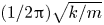 $(1/2 {\rm \pi}) \sqrt {k/m}$ for spring mounted cylinders, but with the constant stiffness
  $k$ replaced by a more complex coefficient, depending on
  $U$ and combining stratification and geometric effects. This frequency can also be written as
 \begin{equation} f_{n} = \frac{U}{2 {\rm \pi}D}\sqrt{\frac{1}{2 Fr^2}+\frac{C_D}{{\rm \pi} l}} . \end{equation}
 The restoring force is due to the combined action of drag and stratification. The natural frequency of the system is thus no longer proportional to  $U$ as for the non-stratified case. Furthermore, for strong stratification
  $f_n$ becomes constant
  $f_n\sim N/(2\sqrt {2}{\rm \pi} )$.
In the general case, the expression of  $U^*$ is
 \begin{equation} U^*= \frac{2 {\rm \pi}}{\sqrt{\dfrac{1}{2 Fr^2}+\dfrac{C_D}{{\rm \pi} l}}} . \end{equation}
 This value is bounded by  $U_0^*$ that is reached for large Froude number. In table 1, the value of
  $U_0^*$ has been indicated for each experimental configuration.
Equation (4.2) provides the natural frequency  $f_n$ but also the oscillator damping rate
  $\sigma _D$ as
 \begin{equation} \sigma_D=\frac{1}{2}\left( \frac{c}{2\rho_0V_{s}}+ \frac{C_D U}{{\rm \pi} D} \right) . \end{equation}
 Measures in still air demonstrate that the damping rate caused by the structure ( $c/(2\rho _0V_{s}) \approx 5\times 10^{-3}\ \textrm {s}^{-1}$) is at least 20 times smaller than the drag-induced hydrodynamic damping term (
 $C_DU/({\rm \pi} D) \geqslant 0.1\ \textrm {s}^{-1}$). The value of
  $\sigma _D$ thus reduces to the second term in (4.9). The damping ratio
  $\zeta = \sigma _D/(2{\rm \pi} f_n)$ is thus close to
  $U^*/4{\rm \pi} ^2$, and therefore always smaller than
  $U_0^*/4{\rm \pi} ^2$ which is at most equal to 1.
In figure 10(a),  $f/f_n$ is plotted vs
  $Fr$. One can see that the upper branch mode now exhibits a constant frequency around
  $2\,f_{n}$, which confirms the link between the observed frequency and the natural frequency of the oscillator.

Figure 10. Frequency of VIV mode as a function of Froude number (a) and  $U^*$ (b). Purple line stands for the Strouhal frequency (
 $St=0.2$). Purple dotted line stands for
  $f^{*}_{{lower}}$ as defined in (1.3). In (b) the lower-frequency mode was removed for clarity.
This result is also in good agreement with the formula (1.3) for the lock-in frequency of the lower branch VIV mode which predicts  $f^*_{{lower}} \approx 2.1$ in the case of low mass ratio. This is clearly visible in figure 10(b), where this value of the theoretical frequency
  $f^*_{{lower}}$ has been indicated with the dashed line. In this figure, where
  $f/f_n$ is plotted vs
  $U^*$, the vortex shedding frequency is also shown by the solid line. A synchronization on the right side of this line is observed, as expected, but for larger values of
  $U^*$ than in classical VIV theory. The large extent of the synchronization range (until
  $U^* \approx 35$) is classical for low-mass-ratio experiments, e.g. Govardhan & Williamson (Reference Govardhan and Williamson2000) predict a lock-out in homogeneous fluids at
  $U^* \approx 19$ in the case
  $m^*=1$. Note that the observed ‘late-
 $U^*$’ synchronization can be explained by the presence of the second oscillation mode (discussed in next § 5) present at small
  $U^*$. It is also not in contradiction to the value of the damping ratio
  $\zeta$ which remains smaller than 1 for all the regimes where oscillations are observed.
In figure 11, the amplitude of the most unstable configurations is plotted as a function of  $U^*$. These configurations correspond to the smallest values of
  $l$, for which the maximal value
  $U_0^*$ of
  $U^*$ is also the smallest. These limits are indicated as vertical dashed lines in the figure. The value of the peak amplitude decreases as
  $U^*$ increases, as expected. But very low amplitudes are also observed for small
  $U^*$ that cannot be explained by the classical VIV theory. It is suspected that, in this regime, for which the Froude number is small, the stratification modifies the flow and the drag and lift forces it exerts on the cylinder.

Figure 11. Amplitude of VIV mode as a function of  $U^*$, for experiments with smaller
  $l$.
$l$.
5. The galloping mode
5.1. Description and interpretation
Below the VIV-like frequency branch, figure 8 shows the existence of a second vibration mode of the system with a constant frequency around  $0.25N/2{\rm \pi}$. This mode occurs at rather low Froude numbers (
 $Fr \in [1;3]$), i.e. when the buoyancy forces are no longer negligible with respect to the inertial forces. Furthermore, it is not observed for small arms, but only when the ratio
  $l$ is larger than a critical value (approximately 7), as will be further discussed in the next section. This indicates that the predominance of buoyancy forces over restoring drag forces is also probably important to observe this mode.
The amplitude of this mode is plotted in figure 12. Despite a strong scatter, the amplitude peak reaches values between one and two cylinder diameters. This is between two and four times the maximal value obtained for VIV modes (see figure 7 and compare figures 11 and 12).

Figure 12. Amplitude of cylinder oscillation in galloping mode as a function of Froude number.
The characteristics of this mode (low-frequency and high-amplitude oscillations) is representative of galloping mode, which occurs in a homogeneous fluid when the axisymmetry of the object is broken. As shown, for example, by Bokaian & Geoola (Reference Bokaian and Geoola1984) in the case of a square cylinder, the galloping mode results from an instability: due to symmetry breaking, a tilt of the cylinder induces a lift in the same direction as the motion, and therefore increases the displacement. This instability leads to very large-amplitude oscillations because they are only limited by the structure itself. Owing to its axisymmetry, no galloping instability appears for a circular cylinder in a homogeneous fluid. However, in the presence of stratification, as the axisymmetry is automatically broken, a destabilizing lift could a priori be generated, even for a circular cylinder. Numerical simulations are presented in the next section to test this possibility.
5.2. Numerical simulations
Numerical simulations are performed using the commercial software COMSOL©. The following configuration is simulated: in a fluid with a linear stratification  $\bar {\rho }$, a cylinder is moved at a constant speed
  $\boldsymbol {U}$, in a direction that makes an angle
  $\alpha$ with respect to the horizontal plane. The total density is written as
  $\rho =\rho _0+\bar {\rho }(z)+\rho '(x,y,z,t)$ where
  $\rho _0 +\bar {\rho }(z)$ is the background fluid density and
  $\rho '$ the density induced by the cylinder displacement. Distances are non-dimensionalized by
  $D$, velocities by
  $U$, pressure by
  $\rho _0 U^2$ and density by
  $\rho _0 D N^2/g$. In the cylinder frame of reference, the Navier–Stokes equations under the Boussinesq approximation and the density transport equation can then be written as
 \begin{gather} \frac{\mathrm{D} \boldsymbol{u}}{\mathrm{D}t} ={-}\boldsymbol{\nabla}p+\frac{1}{Re} \Delta \boldsymbol{u} - \frac{\rho'}{Fr^2}\boldsymbol{e}_{\boldsymbol{z}}, \end{gather}
 \begin{gather}\frac{\mathrm{D} \rho'}{\mathrm{D}t} - (u_z+\sin{\alpha}) = \frac{1}{Re Sc} \Delta \rho' . \end{gather}
 In (5.1b), the  $u_z$ term comes from the density transport due to the linear gradient, and the
  $\sin {\alpha }$ term is associated with the change of frame.
The problem is solved in a  $(x,z)$ domain defined by
  $-5\leqslant x\leqslant 20$ and
  $-5\leqslant z\leqslant 5$ with the cylinder centred at the origin. The angled velocity is imposed at the top (
 $z=5$), the bottom (
 $z=-5$) and the entrance (
 $x=-5$) of the domain. Outlet boundary conditions are imposed at
  $x=20$. Smooth sponge layers of thickness 1 have been added at the top and bottom in order to damp internal waves: the viscosity is multiplied by a factor 1000 in these layers. A small Froude number
  $Fr=1.5$ and an intermediate Reynolds number (
 $Re =300$) are considered such that there is no vortex shedding (Boyer et al. Reference Boyer, Davies, Fernando and Zhang1989). We are interested in the stationary solution to (5.1a,b).
The density and pressure fields of this stationary solution are plotted in figure 13. The resulting vertical force (sum of drag and lift components on  $\boldsymbol {e}_{\boldsymbol {z}}$), shown in figure 14, is calculated by integrating the viscous force and pressure force on the cylinder.

Figure 13. Properties of the stationary perturbation induced by an inclined displacement of the cylinder.  $\alpha = 5^{\circ }$,
  $Fr=1.5$,
  $Re=300$,
  $Sc=1$. (a) Density field (colour map) and streamlines. (b) Pressure field (colour map) and streamlines.

Figure 14. Evolution of the vertical force component  $F_z$ as a function of the imposed tilt angle
  $\alpha$;
  $Fr=1.5$ and
  $Re =300$.
Figure 13(a) shows that the density gradient is asymmetrically perturbed by the cylinder. A strong negative lobe of density is created under and behind the cylinder. This density correction is probably related to the combined action of the lee waves and of the recirculation zone. This negative density lobe induces an asymmetric pressure behind the cylinder since its  $z$ derivative is equal to the density in the absence of motion. Indeed, although the usual positive pressure lobe causing drag is observed in front of the cylinder, figure 13(b) also demonstrates the presence of a negative pressure on the lower right of the cylinder. This induces a downward lift
  $F_z < 0$. Since the cylinder is already going down, this lift reinforces the initial motion, thus an instability develops.
The fact that  $F_z$ should be negative for small positive
  $\alpha$ corresponds in our case to the classical Den Hartog criterion for galloping instability (Den Hartog Reference Den Hartog1932)
 \begin{equation} \frac{\partial C_L}{\partial \alpha}+C_D<0, \end{equation}
requiring in fact that  $\partial F_z/\partial \alpha$ should be negative at small angles. It can be recovered by developing
  $F_z$ around small
  $\alpha$ angles (see Blevins (Reference Blevins1977), for further details).
Figure 14 shows that this destabilization process occurs for angles in the range  $[-40^{\circ },40^{\circ }]$. For larger angles, the drag force is stronger than the lift and the destabilizing mechanism described above is no longer present.
To conclude this section, it was shown by analysing the properties of the perturbation induced by the cylinder motion, that the lift can become destabilizing in the presence of stratification when the displacement is no longer horizontal. The mechanism is therefore very similar to the galloping instability.
The next section focuses on the influence of the non-dimensional parameters defined in § 2.3 on the development of the galloping and VIV analogous modes.
6. Competition between the two regimes
As already mentioned, there are three main non-dimensional parameters characterizing the system: the length ratio  $l$ which specifies the geometry, the Froude number
  $Fr$ which compares buoyancy and inertial forces and the Reynolds number
  $Re$ which characterizes viscous effects. In this section, the influence of these different parameters on the observed mode is evaluated.
All data are plotted as a function of  $Fr$ and
  $l$ in figure 15(a). Each solid circle corresponds to an experiment where a distinct mode has been observed. The colour of the circle is related to the frequency of the mode: red circles correspond to low-frequency galloping modes, while blue circles to high-frequency VIV-like modes. This stability map clearly shows that the galloping mode is limited to the square domain of high-
 $l$ and low-
 $Fr$:
$Fr$:  $l$ must be larger than
  $7$ and
  $Fr$ below
  $3$ for the galloping mode to appear. However, these data cover a large range of Reynolds numbers.

Figure 15. Experimental identification of galloping (in red) and VIV (in blue) modes based on the frequency measurement. Dots stand for performed experiments from which no frequency nor amplitude could be determined. (a) Map in ( $Fr,l$) plane of all data. (b) Map in (
 $Fr,Re$) plane of a reduced set of data (
 $l \in [8,12.5]$).
To evaluate the influence of the Reynolds number, the data are plotted as a function of  $Fr$ and
  $Re$ in figure 15(b) for a reduced range of
  $l$ (
$l$ ( $l\in [8,12.5]$) where both modes are observed. The Reynolds number is found to have a weak impact on the transition between galloping and VIV analogous mode compared to the two other non-dimensional numbers. The transition Froude number between the two modes seems to decrease as the Reynolds number increases. However, it is difficult to quantify precisely the
  $Re$ dependence due the lack of data. Indeed, at transition, amplitudes are very weak and frequencies difficult to measure, so many experiments were not conclusive, causing a gap in the available data.
Nevertheless, from figure 15, it can be inferred that the two main control parameters of the system are the Froude number and the geometric parameter  $l$. This is in agreement with the model that have been developed. It has indeed been shown that stratification is essential for the appearance of the galloping mode, while the parameter
  $l$ affects the drag force that is responsible for the development of the VIV-like mode. Viscosity is not expected to play an important role, especially in the regimes of large
  $Re/Fr$ that have been considered.
7. Conclusion
The classical experiment of a spring-mounted cylinder has been adapted to the case of a stratified fluid: the flowing water channel has been replaced by a towing tank of stratified fluid, and the cylinder has not been mounted on springs but on flat blade-shaped arms free to rotate around their end. With this set-up, drag and buoyancy forces induce a vertical restoring force that mimics the action of a spring.
This pioneered experimental study of FIV in a stratified fluid has brought out the existence of two different oscillating modes for a circular cylinder.
The first one has a moderate amplitude (less than  $0.6D$) and a frequency that can be understood by a classical VIV approach. Indeed, it is proportional to the natural frequency
  $f_n$ of the mechanical system. The lock-in frequency ratio
  $f/f_n$ has been shown to be reasonably well predicted by the classical VIV theory for low mass ratio (Williamson & Govardhan Reference Williamson and Govardhan2004). The natural frequency
  $f_n$ is shown to be not constant. It varies from
  $f_n \sim N/(2\sqrt {2}{\rm \pi} )$ for small Froude numbers to
  $f_n \sim U/2 {\rm \pi}D \sqrt {C_D/{\rm \pi} l}$ for large Froude numbers. In a spring-mounted experiment, this natural frequency would be expected to switch from
  $f_n \sim N/(2\sqrt {2}{\rm \pi} )$ to
  $\sqrt {k/(m^*+C_A)}$ as the spring constant
  $k$ increases.
The second mode is a galloping mode, characterized by a large amplitude (up to  $2D$) and a low frequency close to
  $0.25N/2{\rm \pi}$. It has been linked to the breaking of the axisymmetry due to the stratification. In particular, it has been associated with the presence of a destabilizing lift force, as for the galloping modes of non-cylindrical objects. This mode has been observed for low Froude numbers (
 $Fr \leqslant 3$), and long arms (
 $l \geqslant 7$).
Galloping and VIV modes were also observed in classical VIV systems in a homogeneous fluid when the object is no longer axisymmetric, but the scenario of appearance is different. In general, as  $U^*$ increases, VIV mode appears first, then it is replaced by the galloping mode, that never disappears (Nemes et al. Reference Nemes, Zhao, Lo Jacono and Sheridan2012; Mannini et al. Reference Mannini, Marra and Bartoli2014). Here, the scenario is opposite. We have first observed the galloping mode for small
  $U^*$ and then the VIV-like mode. This can be understood because small values of
  $U^*$ also correspond to small Froude numbers, which are necessary for the existence of the galloping mode. As
  $U^*$ increases,
  $Fr$ also increases, so the buoyancy restoring force responsible for the instability of the galloping mode reduces, and is finally not sufficient to sustain the mode when
  $Fr$ is too large.
The effect of the Reynolds number on the transition from one mode to the other has been analysed for  $Re$ between 500 and 15 000, but no significant dependence has been noticed.
Oceans, which are stratified, are full of cables (transatlantic communications, oil platforms…) subject to complex streams, and then, potentially, the FIV phenomenon. As this study shows a strong influence of stratification on fluid–structure interactions that has never been addressed before, it would be of interest to consider these specific applications. In oceans and seas, the Brünt–Väisälä frequency  $N$ ranges from
  $10^{-3}$ in the deep ocean (Munk Reference Munk1966) to
  $1.5\times 10^{-2}\ \textrm {rad}\ \textrm {s}^{-1}$ in the thermocline of the black sea, for example (Capet et al. Reference Capet, Stanev, Beckers, Murray and Grégoire2016). With the latter value, considering a current of
  $U=0.1\ \textrm {m}\ \textrm {s}^{-1}$, cables of diameter
  $D$ larger than 67 cm have
  $Fr<10$. For such a value of the Froude number, a VIV-like mode leading to non-negligible oscillations of the structure has been observed in this study. In the atmosphere, where
  $N$ is typically of order
  $2\times 10^{-2}\ \textrm {rad}\ \textrm {s}^{-1}$ (Bougeault & Sadourny Reference Bougeault and Sadourny2001), with a wind of velocity
  $U=1 \ \textrm {m}\ \textrm {s}^{-1}$, bridge structures of diameter larger than 5 m may undergo oscillations since the Froude number is below 10.
This study suggests numerous possible further research to fully understand the presented modes. Indeed, the VIV model presented here may be improved by considering the increase of the mean drag with the oscillation amplitude. The fluctuating component of the drag and the lift may also need further investigations to better understand the VIV analogous mode.
Exploring the low- $l$ and low-
 $Fr$ regimes would also be very interesting as these parameters could lead to a VIV-like mode modified by the important variations of the Strouhal number observed for low
  $Fr$.
$Fr$.
Changing parameters such as the inclination angle, the rigidity of the body and analysing the effect of a nonlinear stratification would be interesting in order to perform research closer to real-life systems. Another set-up with springs could also be useful for a better comparison with classical homogeneous VIV results, and to ease results interpretation by separating geometric and flow parameters. Finally, using numerical simulations to explore regimes difficult to reach experimentally, such as low Froude and Reynolds number regimes, could be another interesting research path.
Acknowledgements
The authors would like to thank T. Leweke for fruitful discussions.
Declaration of interests
The authors report no conflict of interest.