


1. Introduction
The collective locomotion of numerous animals is an eye-catching biological phenomenon in nature, such as swarming ants (Couzin Reference Couzin2009), a herd of zebra (Vicsek & Zafeiris Reference Vicsek and Zafeiris2012), fish schools and bird flocks (Herbert-Read Reference Herbert-Read2016). Of particular fascination is that a variety of orderly formations can be self-organized by fish schools and bird flocks without any external force (Lissaman & Shollenberger Reference Lissaman and Shollenberger1970; Ashraf et al. Reference Ashraf, Godoy-Diana, Halloy, Collignon and Thiria2016). Investigating such collective behaviour is important in many scientific fields, including evolutionary biology (Ballerini et al. Reference Ballerini2008), control theory (Cui & Gao Reference Cui and Gao2012), fluid dynamics and engineering (Whittlesey, Liska & Dabiri Reference Whittlesey, Liska and Dabiri2010). Consequently, fish schools and bird flocks have received considerable research attention for several decades (Lissaman & Shollenberger Reference Lissaman and Shollenberger1970; Ashraf et al. Reference Ashraf, Godoy-Diana, Halloy, Collignon and Thiria2016). Why do they travel in the regular aggregation? One of the primary viewpoints is that the collective behaviour is driven by some social traits, such as foraging and protection from predators (Larsson Reference Larsson2012). However, the role of hydrodynamics in such collective behaviour has not been paid enough attention for a long time (Krebs Reference Krebs1976), although fish and birds are living in the flow environment.
Recently, Liao et al. (Reference Liao, Beal, Lauder and Triantafyllou2003) experimentally indicated that a fish was able to save energy by adjusting its gait according to the surrounding flow. It seems to reveal that the flow-mediated interactions are crucial for fish schools and bird flocks. Hereafter, the hydrodynamic effect has been increasingly investigated to understand the collective behaviour of fish schools and bird flocks (Filella et al. Reference Filella, Nadal, Sire, Kanso and Eloy2018). The hydrodynamic advantage has been verified by several experiments with living fish schools and bird flocks (Weimerskirch et al. Reference Weimerskirch, Martin, Clerquin, Alexandre and Jiraskova2001; Portugal et al. Reference Portugal, Hubel, Fritz, Heese, Trobe, Voelkl, Hailes, Wilson and Usherwood2014; Ashraf et al. Reference Ashraf, Bradshaw, Ha, Halloy, Godoy-Diana and Thiria2017). However, the evidence against the hydrodynamic advantage also has been observed in some other experiments (Partridge & Pitcher Reference Partridge and Pitcher1979; Usherwood et al. Reference Usherwood, Stavrou, Lowe, Roskilly and Wilson2011). Consequently, the hydrodynamic function for fish schools and bird flocks is still so far controversial. One of the primary challenges is that the performance analysis of fish schools and bird flocks is hard to conduct, since the number of bodies is huge and the flow-mediated interactions are hard to measure.
In order to simplify the problem and consider the fact that most fish and birds are using flapping fins/wings to generate propulsive forces, fish schools and bird flocks are often simplified as two flapping foils in regular arrangements (Dewey et al. Reference Dewey, Quinn, Boschitsch and Smits2014). It has been indicated that the hydrodynamic benefit can be achieved by flapping foils in a variety of regular arrangements, including the tandem arrangement (Kurt & Moored Reference Kurt and Moored2018), the side-by-side arrangement (Dewey et al. Reference Dewey, Quinn, Boschitsch and Smits2014) and the staggered arrangement (Huera-Huarte Reference Huera-Huarte2018). In the tandem formation, the performance augmentation can be achieved by the upstream body when the separation distance is small (Boschitsch, Dewey & Smits Reference Boschitsch, Dewey and Smits2014). Meanwhile, the performance of downstream foil can be improved when it weaves between vortices that shed from the upstream foil (Muscutt, Weymouth & Ganapathisubramani Reference Muscutt, Weymouth and Ganapathisubramani2017). Moreover, the hydrodynamic benefit depends strongly on the streamwise distance and the phase difference between two foils (Lua et al. Reference Lua, Lu, Zhang, Lim and Yeo2016). In the side-by-side arrangement, the lateral interference can improve the thrust generation and propulsive efficiency of two foils (Dewey et al. Reference Dewey, Quinn, Boschitsch and Smits2014). However, the lateral interference is determined by the phase difference and the lateral distance between two foils (Dong & Lu Reference Dong and Lu2007). When the in-phase motion is used, two parallel foils can reduce the power consumption, as compared with that of a single foil (Dong & Lu Reference Dong and Lu2007). When the anti-phase motion is used, two foils can generate larger thrust than that of a single foil (Dewey et al. Reference Dewey, Quinn, Boschitsch and Smits2014). However, it should be pointed out that in these previous studies, the foils were fixed in the oncoming flow and their motions were prescribed. Namely, these simplified models do not account for the feedback of bodies to the surrounding flow.
Attempting to further understand the collective behaviour of fish schools and bird flocks, the self-propelled model consisting of several flapping foils has been proposed recently (Zhu, He & Zhang Reference Zhu, He and Zhang2014). It has been indicated that the orderly formations can be spontaneously formed via the flow-mediated interactions (Zhu et al. Reference Zhu, He and Zhang2014). For two tandem self-propelled foils, the stable formations can be achieved when the follower intercepts the vortices that shed from the leader (Zhu et al. Reference Zhu, He and Zhang2014; Ramananarivo et al. Reference Ramananarivo, Fang, Oza, Zhang and Ristroph2016). Moreover, the performance of the follower can be significantly improved in the stable formations, as compared with that of a single one (Zhu et al. Reference Zhu, He and Zhang2014). This is different from the observation in the previous studies, in which the fixed tandem foils were used (Muscutt et al. Reference Muscutt, Weymouth and Ganapathisubramani2017). Furthermore, it has been revealed that the emergence of orderly formation depends strongly on the phase difference and the initial distance between two foils (Newbolt, Zhang & Ristroph Reference Newbolt, Zhang and Ristroph2019; Lin et al. Reference Lin, Wu, Zhang and Yang2019b). When the phase difference and the initial distance are appropriate, a compact formation can be formed by the tandem foils, in which both speed and efficiency are increased as compared with those of a single foil (Lin et al. Reference Lin, Wu, Zhang and Yang2019b).
For two foils with an initial side-by-side arrangement, the emergence of an orderly formation is also determined by the phase difference and the initial spacing between two foils (Peng, Huang & Lu Reference Peng, Huang and Lu2018). The staggered-following formation and the alternate-leading formation can be observed in the in-phase scenario, whilst the moving abreast formation and the alternate-leading formation can be observed in the anti-phase scenario (Peng et al. Reference Peng, Huang and Lu2018). As compared with the isolated foil, the higher propulsive efficiency can be achieved by two foils in both staggered-following and moving abreast formations (Peng et al. Reference Peng, Huang and Lu2018). Moreover, for multiple self-propelled foils with different initial arrangements (such as tandem, triangular and diamond arrangements), the stable formations and the performance augmentation still can be achieved via the flow-mediated interactions (Dai et al. Reference Dai, He, Zhang and Zhang2018; Park & Sung Reference Park and Sung2018; Lin et al. Reference Lin, Wu, Zhang and Yang2020). However, it should be noted that the self-propelled model used in the previous studies was free only in the longitudinal direction, but constrained in the lateral direction. Namely, the lateral feedback of foils to the surrounding flow is neglected. As a consequence, when the lateral constraint is cancelled, whether the stable formation can be spontaneously achieved is still an open question.
In fact, individuals in fish schools and bird flocks are unconstrained in both longitudinal and lateral directions. To better understand the collective behaviour of fish schools and bird flocks, the self-propelled model in which foils can self-propel in both longitudinal and lateral directions is considered in this paper. As shown in figure 1, two foils are initially arranged in the side-by-side formation. The most obvious feature of the model used here is that, the self-organizations in both lateral and longitudinal directions are implemented. This is different from the model used in the previous work, in which the self-organization is only considered in the longitudinal direction or not (Dong & Lu Reference Dong and Lu2007; Dewey et al. Reference Dewey, Quinn, Boschitsch and Smits2014; Huera-Huarte Reference Huera-Huarte2018). The specific aim here is to demonstrate that the formation of lateral and longitudinal equilibrium distances can be spontaneously achieved by two flapping swimmers via the hydrodynamic interactions. The remainder of this paper is organized as follows. The problem description and methodology are presented in § 2. The simulation results are addressed in detail with discussion in § 3. Finally, some conclusions are drawn in § 4.

Figure 1. Sketch view of the simulation model. Here  $D_x$ is the longitudinal distance between two foils,
  $D_y$ is the lateral distance between two foils,
  $b$ is the thickness, and
  $c$ is the chord of each foil.
2. Problem description and methodology
As shown in figure 1, the rigid foil that has a semicircular leading edge with diameter  $b=0.1c$ is selected as the profile of the self-propelled flapping foil. Each foil is driven by the harmonic pitching motion in the lateral direction
 \begin{equation} \theta_{i} = \theta_{m}\sin \left( 2{\rm \pi} ft+(i-1)\varphi \right), \end{equation}
where  $\theta _{i}$ is the instantaneous pitching motion of
  $i$th foil (
 $i=1,2$),
  $\theta _{m}$ and
  $f$ are, respectively, the pitching amplitude and frequency,
  $\varphi$ is the phase difference between two foils,
  $t$ is the time. In this paper, the pivot location of each foil is fixed at
  $0.05c$, and its propulsion is controlled by Newton's second law, which can be described as follows (Lin, Wu & Zhang Reference Lin, Wu and Zhang2021):
 \begin{equation} m\frac{\textrm{d}^{2}{\boldsymbol{X}}_i}{\textrm{d}t^{2}} = {\boldsymbol{F}}_i, \end{equation}
where  ${\boldsymbol {X}}_i=(X_i,Y_i)$ is the position vector of the foil,
  ${\boldsymbol {F}}_i=(F_{ix},F_{iy})$ is the hydrodynamic force applied on the foil surface, which results from the hydrodynamic interactions,
  $m=\rho _s s$ is the mass of foil, where
  $\rho _s$ and
  $s$ are, respectively, the density and area of foil. The mass ratio is chosen as
  $\bar {m}=m / m_f=1.0$ in this study, where
  $m_f=\rho s$ is the flow mass with equivalent area and
  $\rho$ is the density of flow. In the current work, the thrust is defined as
  $F_{iT}=-F_{ix}$ and the lateral force is defined as
  $F_{iL}=F_{iy}$. The position and velocity of each foil are, respectively, calculated by using a trapezoidal rule and a forward differencing scheme (Akoz & Moored Reference Akoz and Moored2018), i.e.
 \begin{equation} {\boldsymbol{X}}_i^{t+ \Delta t}={\boldsymbol{X}}_i^{t}+\frac{1}{2}({\boldsymbol{U}}_i^{t+ \Delta t}+{\boldsymbol{U}}_i^{t}) \Delta t,\quad {\boldsymbol{U}}_i^{t+ \Delta t}={\boldsymbol{U}}_i^{t}+\frac{{\boldsymbol{F}}_i^{t}}{m} \Delta t, \end{equation}
where  ${\boldsymbol {U}}_i=(u_{ix}, u_{iy})$ is the velocity of each foil,
  $\Delta t$ is the time step, the superscripts ‘
 $t$’ and ‘
 $t+ \Delta t$’ represent the variables at time instants
  $t$ and
  $t+ \Delta t$. The cycle-averaged speed of each foil can be calculated as
 \begin{equation} \bar{u}_{ix} = \frac{1}{T} \int_0^{T} {u_{ix}}\,\textrm{d}t,\quad \bar{u}_{iy} = \frac{1}{T} \int_0^{T} {u_{iy}} \,\textrm{d}t, \end{equation}
where  $T$ is the flapping period. Meanwhile, the cycle-averaged power consumption of each foil is defined as
 \begin{equation} \bar{P}_i = \frac{1}{T} \int_0^{T} \left( M_i (\textrm{d}\theta_i/\textrm{d}t) \right) \textrm{d}t, \end{equation}
where  $M_i$ is the torque applied on each foil surface. The propulsive efficiency of the two-foil system is defined as the ratio of the kinetic energy obtained by the foils to the work done to the fluid by the foils in one flapping cycle (Park & Sung Reference Park and Sung2018; Peng et al. Reference Peng, Huang and Lu2018), which can be calculated as
 \begin{equation} \boldsymbol{\eta} = \frac{\sum_{i=1}^{2} \bar{E}_{ik}}{\sum_{i=1}^{2} \left(\bar{P}_i T \right)}, \end{equation}
where  $\bar {E}_{ik}=m(\bar {u}_{ix}^{2}+\bar {u}_{iy}^{2})/2$ is the cycle-averaged kinetic energy of each foil.
The surrounding flow of the flapping foils is considered to be incompressible and viscous, which is governed by the Navier–Stokes equations as follows:
 \begin{gather} \frac {\partial {\boldsymbol{u}}}{\partial t} + {\boldsymbol{u}} \boldsymbol{\cdot} \boldsymbol{\nabla} {\boldsymbol{u}} ={-}\frac {1}{\rho} \boldsymbol{\nabla} p + \nu \nabla^{2} {\boldsymbol{u}}, \end{gather}
 \begin{gather}\boldsymbol{\nabla} \boldsymbol{\cdot} {\boldsymbol{u}}=0, \end{gather}
where  ${\boldsymbol {u}}$ is the flow velocity vector,
  $p$ is the pressure,
  $\nu$ is the kinematic viscosity of flow. A simplified circular function-based gas kinetic method (Yang et al. Reference Yang, Shu, Yang, Wang and Wu2017) is used to solve the Navier–Stokes equations, and the implicit velocity correction-based immersed boundary (Wu & Shu Reference Wu and Shu2009) is used to resolve the interaction between the flapping foils and the surrounding flow. For more details about the numerical method adopted, please refer to our previous work (Wu & Shu Reference Wu and Shu2009; Yang et al. Reference Yang, Shu, Yang, Wang and Wu2017; Lin et al. Reference Lin, Guo, Wu and Nan2018; Lin, Wu & Zhang Reference Lin, Wu and Zhang2019a).
In order to validate the adopted numerical method and the corresponding code, the flapping foil problem used in previous work (Wang, Birch & Dickinson Reference Wang, Birch and Dickinson2004) is selected, in which the stationary flow condition is the same as that in the current work. The results obtained with the same controlled parameters as those in the study of Wang et al. (Reference Wang, Birch and Dickinson2004) are illustrated in figure 2(a,b), it is clear that the present results agree well with the experimental and numerical results in study of Wang et al. (Reference Wang, Birch and Dickinson2004). Consequently, the adopted method is suitable for the current study. Furthermore, a sensitivity test is conducted. The time histories of the separation distances between two foils are illustrated in figure 3. It can be seen that the result obtained from the mesh of  $\Delta x=0.01c$ is very close to that obtained from the mesh of
  $\Delta x=0.005c$. To strike a balance between computational expense and accuracy that is related to the mesh, a mesh of
  $\Delta x=0.01c$ is chosen for the current simulations. In this study, the length is non-dimensionalized with
  $c$, the time is scaled by
  $10^{-2} c^{2}/(2 \nu )$, the velocity is non-dimensionalized with
  $U=10^{2} \nu / (0.5c)$, the force is scaled by
  $10^{4}\rho \nu ^{2}/(0.5c)$ and the power is scaled by
  $10^{6} \rho \nu ^{3} /(0.25c^{2})$ (Lin et al. Reference Lin, Wu and Zhang2021). In addition, the Reynolds number is set to be
  $Re=Uc/\nu =200$ in this work.

Figure 2. Comparisons of (a) lift and (b) drag coefficients of a flapping foil with previous results.

Figure 3. Time histories of the separation distances in (a) the  $x$-direction and (b) the
  $y$-direction between two foils obtained from different mesh spacing. The flapping parameters are
  $f=1$,
  $\theta _{m}=15^{\circ }$,
  $\varphi =0$.
3. Results and discussion
In this paper, the self-organization of two flapping foils that can self-propel in both the  $x$- and
  $y$-directions is numerically investigated. The controlled parameters used in the current work are listed in table 1. It can be seen that five parameters are variables: the initial lateral distance (
 $D_{y0}$), the initial longitudinal distance (
 $D_{x0}$), the pitching frequency (
 $\,f$), the amplitude (
 $\theta _m$) and the phase difference (
 $\varphi$). Considering the phase difference observed in the real fish schools (Ashraf et al. Reference Ashraf, Godoy-Diana, Halloy, Collignon and Thiria2016), two typical scenarios are considered in this study, i.e. in-phase and anti-phase.
Table 1. Values of the controlled parameters used in the current simulations.

3.1. The in-phase scenario
3.1.1. Emergence of staggered formation
First, the performance of two in-phase flapping foils is studied ( $D_{x0}=0, d_{y0}=1.0, \varphi =0$). As shown in figure 4(a,b), it can be seen that the longitudinal distance (
 $D_x$) dramatically increases during the early stage, but the lateral distance (
 $D_y$) decreases sharply. This occurs because the flow-mediated interactions lead to different speeds of the two foils during the early stage. As shown in figure 4(c) for example, for the case of (
 $f=1.0, \theta _m=15^{\circ }$), the longitudinal speed of foil 1 is smaller than that of foil 2 when
  $t/T=18\text {--}28$, but it is larger than that of foil 2 when
  $t/T=28\text {--}32$. Moreover, the lateral speed of foil 1 is negative during the early stage, but that of foil 2 is positive. Namely, two foils move towards each other in the
  $y$-direction during the early stage. After some periods, the two foils achieve the same cycle-averaged longitudinal and lateral speeds, and then
  $D_x$ and
  $D_y$ vary periodically. It is surprising that the equilibrium separation distance in the lateral direction can be spontaneously achieved by two flapping swimmers, together with the longitudinal equilibrium distance. Moreover, it can be seen that both
  $D_x$ and
  $D_y$ are smaller than one chord length. Namely, the staggered formation has been spontaneously formed.

Figure 4. Time histories of the separation distances in (a) the  $x$-direction and (b) the
  $y$-direction between two foils. (c) The cycle-averaged speed and (d) trajectories of the pivot point of two foils in the case of
  $f=1$,
  $\theta _{m}=15^{\circ }$,
  $\varphi =0$.
In the staggered formation, the velocity enhancement can be achieved by two foils as compared with the isolated foil (as shown in figure 4c), and it will be discussed in detail in the following section. Moreover, there is lateral speed for each foil. Consequently, the propulsion trajectory of each foil is deflected. As shown in figure 4(d) for example, there is a deflected angle  $\phi$ between the trajectory of the two-foil system and the longitudinal axis. This is different from the propulsion of the isolated foil, in which no yaw motion happens (the yaw angle of a single foil is smaller than
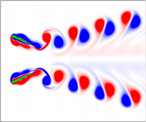
  $0.5^{\circ }$ for the parameters considered here). This occurs because there exist asymmetric hydrodynamic interactions between two staggered foils, as shown in figure 5, for example. The trailing edge vortex V1 shed from foil 2 in the prior period is captured by foil 1, as shown in figure 5(a). Then, it merges with the trailing edge vortex U1 of foil 1, as shown in figures 5(b) to 5(d). A similar vortex capture and merger also can be observed for the other trailing edge vortex of foil 2, such as V2 in figure 5. Consequently, there is only one reversed von Kármán vortex street behind the follower. In addition, it should be pointed out that the similar hydrodynamic interaction and yaw motion can be observed in the other cases, in which the staggered formation has been observed. For more details, please refer to supplementary movie 1 available at https://doi.org/10.1017/jfm.2020.1143.

Figure 5. Instantaneous vorticity contours of two freely self-propelled foils in the staggered formation at time  $t/T=$ (a) 68.1, (b) 68.25, (c) 68.5, (d) 68.75. The parameters are
  $f=1$,
  $\theta _{m}=15^{\circ }$,
  $\varphi =0$.
Furthermore, the stability of the staggered formation needs to be studied. As shown in figure 6, it is clear that the ultimate staggered formation can be achieved by two foils with different values of  $D_{y0}$ and
  $D_{x0}$. Namely, the ultimate staggered formation is independent of
  $D_{x0}$ and
  $D_{y0}$, when the perturbation is small (for example,
  $D_{x0} \leqslant 1.5$ and
  $D_{y0} \leqslant 2.0$). This is different from the result in the previous studies (Park & Sung Reference Park and Sung2018; Peng et al. Reference Peng, Huang and Lu2018), which pointed out that the ultimate formation is determined by
  $D_{y0}$. The reason may be that the self-organization in the lateral direction was not considered in the previous studies (Park & Sung Reference Park and Sung2018; Peng et al. Reference Peng, Huang and Lu2018). Similar to the longitudinal self-organization of two foils (Zhu et al. Reference Zhu, He and Zhang2014; Ramananarivo et al. Reference Ramananarivo, Fang, Oza, Zhang and Ristroph2016; Lin et al. Reference Lin, Wu, Zhang and Yang2019b), when the self-organization in the lateral direction is considered, the equilibrium separation distance in the lateral direction can be achieved by two foils via the hydrodynamic interactions. By the way, it should be noted that two foils would perform like a single foil when
  $D_{x0}$ and
  $D_{y0}$ become large enough.

Figure 6. Time histories of the separation distances between two foils with different values of (a,b) initial lateral distance and (c,d) initial longitudinal distance. The parameters are  $f=1$,
  $\theta _{m}=15^{\circ }$,
  $\varphi =0$.
However, the staggered formation depends strongly on the pitching frequency and amplitude. As shown in figure 7, the staggered formation is only observed in part of the region of the parameter space that considered here. When the pitching parameters are located in the grey region in figure 7, the two-foil system is unable to form a stable formation. For example, the collision between two foils can be observed in most of the grey region in figure 7, which results in the stopping of the simulation immediately. In this paper, only the stable formation will be discussed in detail.

Figure 7. Phase diagram for the staggered formation on the  $f-\theta _{m}$ plane, the red circular symbol represents the staggered formation, and the grey triangle symbol represents the case which is unable to form the stable formation.
3.1.2. Collective performance for staggered formation
The propulsive velocity, the power consumption and the propulsive efficiency are three key parameters quantifying the performance of the flapping swimmer. In this section, the ratios of the cycle-averaged propulsive speed, the cycle-averaged power consumption and the propulsive efficiency of the two-foil system to those of a single foil are examined. To make a comparison, the cycle-averaged power consumption of the two-foil system is calculated as the mean value of each foil, i.e.  $\bar {P}=(\bar {P}_1+\bar {P}_2)/2$. In the stable formation, two foils have the same cycle-averaged speed in both longitudinal and lateral directions, i.e.
  $\bar {u}_x=\bar {u}_{1x}=\bar {u}_{2x}$ and
  $\bar {u}_y=\bar {u}_{1y}=\bar {u}_{2y}$. Since the cycle-averaged lateral speed of a single foil is approximately zero, only the longitudinal speed of two staggered foils is selected for comparison.
As shown in figure 8(a), the longitudinal speed of each foil is significantly increased, as compared with that of the isolated foil. However, the power consumption of each foil is larger than that of a single foil, as shown in figure 8(b). As a result, both augmentation and reduction of efficiency can be observed for two foils in the staggered formation, as compared with that of the isolated foil. As shown in figure 8(c), which situation occurs depends on the flapping parameters. Here we define the flapping Reynolds number (Gazzola, Argentina & Mahadevan Reference Gazzola, Argentina and Mahadevan2014), i.e.  $Re_f=fAc/\nu$, where
  $A=1.9\sin (\theta _m)$ is the peak-to-peak amplitude of the pitching foil. As shown in figure 8(d), when the flapping Reynolds number is small (approximately
  $Re_f<65$, the orange region in figure 8d), the propulsive efficiency of the two-foil system is smaller than that of a single foil. Instead, the propulsive efficiency of the two-foil system is larger than that of a single foil as the flapping Reynolds number is increased (approximately
  $Re_f>65$, the purple region in figure 8d).

Figure 8. Ratios of cycle-averaged (a) longitudinal speed, (b) power consumption and (c) efficiency of the staggered foils to those of the isolated foil. The subscript ‘ $s$’ denotes the isolated foil, and the same below. (d) The relationship between the efficiency ratio and the flapping Reynolds number.
Moreover, we can define two Reynolds numbers, respectively, based on the longitudinal speed and the lateral speed of each foil, i.e.  $Re_{ux}=\bar {u}_xc/\nu$ and
  $Re_{uy}=\bar {u}_yc/\nu$. As shown in figure 9(a,b), it can be seen that both
  $Re_{ux}$ and
  $Re_{uy}$, respectively, can be couched as two simple scaling laws of
  $Re_{ux} \sim Re_f^{1.8}$ and
  $Re_{uy} \sim Re_f^{3.2}$. Similar to the scaling law of a single swimmer (Gazzola et al. Reference Gazzola, Argentina and Mahadevan2014; Lin et al. Reference Lin, Wu and Zhang2021), our results seem to indicate that the speed of multiple swimmers in the collective behaviour also can be couched as a simple scaling law. Moreover, it can be seen from figure 9(a) that, as compared with the performance of a single foil, the hydrodynamic benefit of the collective behaviour of two foils is enhanced as
  $Re_f$ increases. However, it should be pointed out that the universality of such scaling laws is still unknown, and it may not be valid if the flow condition (such as the Reynolds number) is significantly changed.

Figure 9. The propulsive Reynolds number in (a) the  $x$-direction and (b) the
  $y$-direction as a function of the flapping Reynolds number. The blue dash-dot-dot line in panel (a) represents the scaling law for the isolated foil, which is illustrated in the inset.
In order to further study the unsteady dynamics of two foils in the staggered formation, the case with pitching parameters of  $f=1.0$ and
  $\theta _m=15^{\circ }$ is selected as a typical example for analysis. The time histories of propulsive velocity of two foils in one pitching period are illustrated in figure 10. It can be seen from figure 10(a) that both
  $u_{1x}$ and
  $u_{2x}$ are larger than
  $u_{sx}$ during the whole period. On the other hand, it can be seen from figure 10(b) that the magnitude of the peak in
  $u_{1y}$ is smaller than that in
  $u_{sy}$. Meanwhile, the magnitude of the trough in
  $u_{2y}$ is larger than that in
  $u_{sy}$. The differences in the magnitude of peak and trough of both
  $u_{1y}$ and
  $u_{2y}$ are obvious, which leads to the lateral propulsion for each foil. In addition, it can be seen that the developments of
  $u_{1x}$ and
  $u_{1y}$ are, respectively, different from
  $u_{2x}$ and
  $u_{2y}$, even though they are driven by the same pitching motion. This occurs because there exist asymmetric hydrodynamic interactions between two foils, which induce the asynchronized hydrodynamic forces, as shown in figure 10(c,d). It can be described as follows.

Figure 10. Time histories of (a) longitudinal speed, (b) lateral speed, (c) thrust and (d) lateral force of two foils in the staggered formation in one period. The parameters are  $f=1$,
  $\theta _{m}=15^{\circ }$,
  $\varphi =0$.
Since the foil here is free in the lateral direction, there exists a passive oscillation for each foil in the lateral direction. The pivot point of each foil moves downwards when it is pitching upwards, and vice versa, as shown in figure 10(b). For instance at  $t/T=68.1$, when each foil is pitching upwards, its pivot point is moving downwards due to the hydrodynamics. Consequently, the former part of foil 1 and the latter part of foil 2 are close to each other, which induces a high positive pressure region between the two foils, as shown in figure 11(a). Such a region can generate an upward repulsion effect on foil 1, and a downward repulsion effect on foil 2, as denoted by the arrows in figure 11(a). Thus, the thrust and lateral force of foil 1 are increased, but those of foil 2 are decreased. As a result, the thrust and lateral force of foil 1 are larger than those of foil 2, as shown in figure 10(c,d).

Figure 11. Instantaneous pressure contours of two foils in the staggered formation at time  $t/T=$ (a) 68.1, (b) 68.25, (c) 68.5, (d) 68.75. The parameters are
  $f=1$,
  $\theta _{m}=15^{\circ }$,
  $\varphi =0$.
When two foils begin to pitch downwards from the peak position, for example at  $t/T=68.25$, the pivot point of each foil starts to move upwards. Thus, the former part of foil 1 and the latter part of foil 2 are going away from each other, which induces a high negative pressure region between the two foils, as shown in figure 11(b). Such a region can generate a downward suction effect on foil 1, but an upward suction effect on foil 2, as indicated by the arrows in figure 11(b). Consequently, the thrust and lateral force of foil 1 are decreased, but those of foil 2 are increased. So the thrust and lateral force of foil 2 are larger than those of foil 1, as shown in figure 10(c,d).
At  $t/T=68.5$, two foils are pitching downwards through the equilibrium position. Since the leading edge vortex of foil 1 is weakened as compared with that of foil 2, as shown in figure 5(c), then the negative pressure region at the head of foil 1 is weakened, as shown in figure 11(c). Therefore, the suction effect of the leading edge vortex of foil 1 is weakened as compared with that of foil 2. As a result, the thrust of foil 1 is smaller than that of foil 2, as shown in figure 10(c). Moreover, when two foils begin to pitch upwards from the lowest position, e.g. at
  $t/T=68.75$, the pivot point of each foil starts to move downwards. Consequently, the front part of foil 1 and the latter part of foil 2 are close to each other again, which induces a high positive pressure region between the two foils. Such a region is good for the lateral force generation of foil 1 and the thrust generation of foil 2, but it is bad for the thrust generation of foil 1 and the lateral force generation of foil 2, as shown by the arrows in figure 11(d). Therefore, the thrust of foil 1 is smaller than that of foil 2, but the lateral force of foil 1 is larger than that of foil 2, as shown in figure 10(c,d).
3.2. The anti-phase scenario
3.2.1. Emergence of side-by-side formation
Phase difference can be generally observed in fish schools and bird flocks (Portugal et al. Reference Portugal, Hubel, Fritz, Heese, Trobe, Voelkl, Hailes, Wilson and Usherwood2014; Ashraf et al. Reference Ashraf, Godoy-Diana, Halloy, Collignon and Thiria2016, Reference Ashraf, Bradshaw, Ha, Halloy, Godoy-Diana and Thiria2017), which means that the phase difference may be important for the collective behaviour. Ashraf et al. (Reference Ashraf, Godoy-Diana, Halloy, Collignon and Thiria2016) reported that the synchronization of two fish can be characterized by in-phase and anti-phase states, and the fish pair favours the anti-phase state. Therefore, the anti-phase scenario is studied here. As shown in figure 12(a),  $D_x$ in the anti-phase scenario is approximately zero throughout, but
  $D_y$ varies dramatically during the early stage. Meanwhile,
  $\bar {u}_{1x}$ and
  $\bar {u}_{2x}$ are synchronized from beginning to end, but
  $\bar {u}_{1y}$ and
  $\bar {u}_{2y}$ are fluctuating during the early stage, as shown in figure 12(b), for example. After several periods,
  $\bar {u}_{1x}$ and
  $\bar {u}_{2x}$ converge to a constant,
  $\bar {u}_{1y}$ and
  $\bar {u}_{2y}$ converge to zero. Therefore,
  $D_y$ varies periodically, i.e. the side-by-side formation is spontaneously formed. Moreover, two foils in the side-by-side formation can self-propel in a straight line, as shown in figure 12(c). This occurs because the side-by-side formation is a symmetric formation, which results in symmetric hydrodynamic interactions between two foils. As shown in figure 13, for example, two foils in the side-by-side formation behave as a jellyfish-like swimmer (Fang et al. Reference Fang, Ho, Ristroph and Shelley2017). The deflected reversed von Kármán vortex street can be observed behind each foil. More details about the propulsion of two foils in the side-by-side formation can be found in supplementary movie 2.

Figure 12. (a) Time histories of the separation distances between two foils. (b) The cycle-averaged speed and (c) trajectories of the pivot point of two foils in the case of  $f=2$,
  $\theta _{m}=25^{\circ }$,
  $\varphi ={\rm \pi}$. (d) Phase diagram for the side-by-side formation on the
  $f-\theta _{m}$ plane, the red diamond symbol represents the side-by-side formation, and the grey triangle symbol represents the case that is unable to form the stable formation.

Figure 13. Instantaneous vorticity contours of two freely self-propelled foils in the side-by-side formation at time  $t/T=$ (a) 90.25, (b) 90.50, (c) 90.75, (d) 91.00. The parameters are
  $f=2$,
  $\theta _{m}=25^{\circ }$,
  $\varphi ={\rm \pi}$.
Similar to the staggered formation, the side-by-side formation also strongly depends on the pitching parameters. As shown in figure 12(d), the side-by-side formation is only observed in a part of the region of the parameter space (the red diamond symbols). Once more, the stability of the ultimate formation is studied. As shown in figure 14, the same side-by-side formation still can be observed when different values of  $D_{x0}$ and
  $D_{y0}$ are selected. Consequently, the ultimate side-by-side formation is independent of
  $D_{x0}$ and
  $D_{y0}$, when the perturbation is small (for example,
  $D_{x0} \leqslant 0.75$ and
  $D_{y0} \leqslant 2.0$).

Figure 14. Time histories of the separation distances between two foils with different values of (a) initial longitudinal distance and (b) initial lateral distance. The parameters are  $f=2$,
  $\theta _{m}=25^{\circ }$,
  $\varphi ={\rm \pi}$.
3.2.2. Collective performance for side-by-side formation
In order to further study the propulsive performance of two foils in the side-by-side formation, the relative difference of performance between the two-foil system and a single foil is calculated, i.e.  $\varDelta \langle \bullet \rangle = ({ \langle \bullet \rangle - \langle \bullet \rangle _s})/{ \langle \bullet \rangle } \times 100\,\%$, where
  $\langle \bullet \rangle$ is the key parameter that quantifies the propulsive performance of the flapping swimmer (i.e. the cycle-averaged velocity, power consumption and efficiency), the subscript ‘
 $s$’ means the isolated foil. As shown in figure 15(a), it can be seen that in the side-by-side formation, the longitudinal speed of the two-foil system is larger than that of a single foil. Moreover, the propulsive efficiency of the two-foil system is higher than that of a single foil, although more power is consumed in some cases, as shown in figure 15(b,c). In addition, it can be seen from figure 15(d) that the propulsive speed of two foils in the side-by-side formation also can be couched as a simple scaling law of
  $Re_{ux} \sim Re_f^{1.56}$. Furthermore, as compared with the performance of the isolated foil, the hydrodynamic benefit of the collective behaviour of two foils in the side-by-side formation is reduced as
  $Re_f$ increases.

Figure 15. The relative difference of (a) propulsive speed, (b) power consumption, (c) propulsive efficiency between two foils in the side-by-side formation and a single foil. (d) The propulsive Reynolds number as a function of the flapping Reynolds number, the blue dash-dot-dot line represents the scaling law for the isolated foil.
To further quantitatively describe the unsteady dynamics of two foils in the side-by-side formation, the case with pitching parameters of  $f=2$ and
  $\theta _m=10^{\circ }$ is selected as a typical example. The time histories of longitudinal speed (
 $u_x$) and thrust (F T) of the two-foil system are, respectively, illustrated in figure 16(a,b), it is clear that both
  $u_x$ and
  $F_T$ of two foils are, respectively, synchronized. In addition,
  $u_x$ of the two-foil system is larger than that of a single foil primarily in the second half-duration of one period, as shown in figure 16(a). The possible reason is that the thrust of the two-foil system is increased in the first half-duration of one period (which can lead to more acceleration), as compared with that of a single foil, but it is decreased in the second half-duration of one period, as shown in figure 16(b).

Figure 16. Time histories of (a) longitudinal speed, and (b) thrust of two foils in the side-by-side formation in one period. The parameters are  $f=2$,
  $\theta _{m}=10^{\circ }$,
  $\varphi ={\rm \pi}$.
Moreover, the instantaneous pressure contours of two foils at the moments of  $t/T=90.25$ and
  $90.75$ are, respectively, illustrated in figure 17(a,b). It is clear that the pressure distribution here is different from that of the fixed foils (Raspa, Godoy-Diana & Thiria Reference Raspa, Godoy-Diana and Thiria2013) and the longitudinal self-propelled foils (Peng et al. Reference Peng, Huang and Lu2018). In previous studies, there exists a high positive pressure region between two foils when they move toward each other, but a high negative pressure region when they move away from each other (Raspa et al. Reference Raspa, Godoy-Diana and Thiria2013; Peng et al. Reference Peng, Huang and Lu2018). However, for the self-propelled foils here, when they move toward each other (e.g.
  $t/T=90.25$), there exists a positive high pressure region between the latter parts of two foils, but a high negative pressure region between the former parts of two foils, as shown in figure 17(a). When they move away from each other (e.g.
  $t/T=90.75$), there is a high positive pressure region between the former parts of two foils, but a negative high pressure region between the latter parts of two foils, as shown in figure 17(b). Such a pressure distribution is the result of the passive oscillation and the driven motion of each foil in the lateral direction.

Figure 17. Instantaneous pressure contours of two foils in the side-by-side formation at time  $t/T=$ (a) 90.25 and (b) 90.75. The parameters are
  $f=2$,
  $\theta _{m}=10^{\circ }$,
  $\varphi ={\rm \pi}$.
3.3. The mechanism behind the stable formations
As presented above, the staggered formation is only observed in the in-phase scenario, and the side-by-side formation is only observed in the anti-phase scenario. In this section, we will explain the mechanism behind the different stable formations.
For the staggered formation, as shown in figure 4(a,b), it can be seen that  $D_y$ is dramatically decreased and
  $D_x$ is significantly increased until the staggered formation is formed. The reason why
  $D_y$ reduces is that the effective angle of attack of each foil in the upstroke is different from that in the downstroke. The effective angle of attack of each foil can be calculated as
  $\alpha _i=a\tan (u_{iy}/u_{ix})-\theta _i$ (Kinsey & Dumas Reference Kinsey and Dumas2008). As shown in figure 18(a), it can be seen that the magnitude of the trough in
  $\alpha _1$ is larger than that in
  $\alpha _2$. Meanwhile, the magnitude of the peak in
  $\alpha _1$ is smaller than that in
  $\alpha _2$. Here the asymmetry in
  $\alpha _i$ is obvious. The cycle-averaged value of
  $\alpha _1$ is negative, and that of
  $\alpha _2$ is positive. For example, when
  $t/T=19\text {--}20$, as shown in figure 18(a),
  $\bar {\alpha }_1=-0.8^{\circ }$ and
  $\bar {\alpha }_2=0.9^{\circ }$, where
  $\bar {\alpha }_i=({1}/{T}) \int _0^{T} \alpha _i \,\textrm {d}t$. Consequently, foil 1 experiences a negative lateral force, but foil 2 experiences a positive lateral force, which results in a negative
  $\bar {u}_{1y}$ and a positive
  $\bar {u}_{2y}$, as shown in figure 4(c). As a result, two foils move toward each other, i.e.
  $D_y$ reduces, as shown in figure 4(b).

Figure 18. Time histories of (a) the effective angle of attack, (b) the thrust and (c) the longitudinal speed of two foils in one period in the case of  $f=1$,
  $\theta _{m}=15^{\circ }$,
  $\varphi =0$. (d) Time histories of the separation distances in both the
  $x$- and
  $y$-directions between two foils that are driven by
  $\theta =\theta _{m}\sin (2{\rm \pi} ft+{\rm \pi} )$.
The reason why  $D_x$ increases is that the effects of flow-mediated interactions on two foils are unsynchronized in the in-phase scenario. As shown in figure 18(b), the thrust of foil 2 is larger than that of foil 1 during the first half of the period. Thus, the speed of foil 2 is increased more sharply than that of foil 1, as shown in figure 18(c). Consequently, foil 2 can outstrip foil 1 during the first half of the period. In the second half of the period, the thrust of foil 1 is increased as compared with foil 2, and the speed of foil 1 is increased more sharply than that of foil 2. However, since foil 2 has been partially ahead of foil 1 in the first half of the period, the region in which two foils interacting each other in the second half of the period is smaller than that in the first half of the period. Thus, the interference interaction is weakened in the second half of the period, as compared with that in the first half of the period. Consequently, it is clear that the difference in the magnitude of
  $F_{1T}$ and
  $F_{2T}$ in the first half of the period is larger than that in the second half of the period, as shown in in figure 18(b). Therefore, the mean longitudinal speed of foil 2 is larger than that of foil 1, for example
  $\bar {u}_{1x}=0.15$ and
  $\bar {u}_{2x}=0.18$ in the duration of
  $t/T=19-20$. Consequently, foil 2 can always be ahead of foil 1, i.e.
  $D_x$ increases.
As discussed above, the foil that firstly gets benefit from the interference interaction between two foils can stay ahead of the other one. Considering the fact that foil 2 swims ahead of foil 1 in all the cases in which the staggered formation can be observed, we hypothesize that which foil becomes the leader in the staggered formation depends on the driven motion. For example, if two foils are driven by  $\theta = \theta _{m}\sin \left ( 2{\rm \pi} ft+ {\rm \pi}\right )$, foil 1 can firstly achieve the thrust enhancement, and then it can outstrip foil 2. Thus, the staggered formation in which foil 1 swims ahead of foil 2 can be observed. To validate the hypothesis, some cases are simulated, as shown in figure 18(d), the result agrees well with our hypothesis.
However, for the anti-phase scenario, since the driven motions of two foils are symmetric, the effects of flow-mediated interactions on two foils are synchronized. As shown in figures 12(b) and 16(a,b), the thrust and longitudinal speed of two foils are synchronized. Thus,  $D_x$ can remain zero from beginning to end in the anti-phase scenario, as shown in figure 12(a). This is the reason why the side-by-side formation, instead of the staggered formation, has been observed in the anti-phase scenario.
4. Conclusions
In summary, the self-organization of two parallel flapping foils, which can self-propel in both the longitudinal and the lateral directions, is numerically studied in this paper. The results indicate that the equilibrium positions in both lateral and longitudinal directions can be spontaneously achieved by two foils via hydrodynamic interactions. To our knowledge, it is the first numerical confirmation that two flapping swimmers can simultaneously converge to equilibrium distances in both the lateral and the longitudinal directions. In addition, two types of stable formations have been observed, and which type occurs depends on the phase difference. The staggered formation has been observed in the in-phase scenario, and the side-by-side formation has been observed in the anti-phase scenario. Moreover, the emergence of each stable formation is independent of the perturbation of initial distances when the perturbation is small, but strongly depends on the pitching frequency and amplitude.
In the staggered formation, considerable velocity enhancement can be achieved by the two-foil system, but at the cost of more power consumption, as compared with a single foil. Moreover, two foils in the staggered formation can generate a yawing motion, since the hydrodynamic interactions between them are asymmetric. In the side-by-side formation, both velocity and efficiency of the two-foil system are enhanced, as compared with those of a single foil. Moreover, each foil in the side-by-side formation can keep self-propelling in a straight line, i.e.  $\bar {u}_y \approx 0$. In addition, the locomotory dynamics of two foils in the stable formations are governed by some simple scaling laws. Namely,
  $Re_{ux} \sim Re_f^{1.8}$ and
  $Re_{uy} \sim Re_f^{3.2}$ for two foils in the staggered formation, and
  $Re_{ux} \sim Re_f^{1.56}$ for two foils in the side-by-side formation. The results obtained here can shed some light on the understanding of the collective behaviour of biological bodies, and may be useful for the optimization of the coordinated locomotion of multiple aerial/underwater microrobots.
Finally, it should be pointed out that the Reynolds number in this work is smaller than that of the real swimmer school (Huntley & Zhou Reference Huntley and Zhou2004; Fukuda et al. Reference Fukuda, Torisawa, Sawada and Takagi2010). The parameter space in which the stable formations can be observed and the scaling laws may be changed when the Reynolds number is increased. Moreover, except the in-phase and anti-phase scenarios considered here, the staggered formation and the side-by-side formation could be observed when the phase difference is set to be other appropriate values. However, the effects of the Reynolds number and the phase difference on the collective performance of two freely flapping swimmers are just neglected in the current work, and it is worthwhile to conduct a deeper study in the future.
Supplementary movies
Supplementary movies are available at https://doi.org/10.1017/jfm.2020.1143.
Funding
J.W. acknowledges the support of the National Natural Science Foundation of China (grant no. 12072158) and the Research Fund of State Key Laboratory of Mechanics and Control of Mechanical Structures (Nanjing University of Aeronautics and Astronautics) (grant no. MCMS-I-0120G02). X.L. acknowledges the support of the Funding for Outstanding Doctoral Dissertation in NUAA (grant no. BCXJ19-02) and Postgraduate Research & Practice Innovation Program of Jiangsu Province (grant no. KYCX19_0154). This work is also supported by the Priority Academic Program Development of Jiangsu Higher Education Institutions (PAPD).
Declaration of interests
The authors report no conflict of interest.


