


1. Introduction
Vortex shedding from the leading edges of foils, wings and rotor blades have been observed in nature – on swimming and flying animals and seeds (Ellington et al. Reference Ellington, van den Berg, Willmott and Thomas1996; Taylor, Nudds & Thomas Reference Taylor, Nudds and Thomas2003; Muijres et al. Reference Muijres, Johansson, Barfield, Wolf, Spedding and Hedenström2008; Lentink et al. Reference Lentink, Dickson, Van Leeuwen and Dickinson2009; Limacher & Rival Reference Limacher and Rival2015; Bottom II et al. Reference Bottom, Borazjani, Blevins and Lauder2016), and in engineering – on rotorcraft (Carr Reference Carr1988; Corke & Thomas Reference Corke and Thomas2015), wind turbines (Schreck & Robinson Reference Schreck and Robinson2005), swept and delta wings (Maltby Reference Maltby1968; Hitzel & Schmidt Reference Hitzel and Schmidt1984; Gursul, Gordnier & Visbal Reference Gursul, Gordnier and Visbal2005), micro-air vehicles (Ellington et al. Reference Ellington, van den Berg, Willmott and Thomas1996; Ellington Reference Ellington1999) and flapping-wing energy-harvesting devices (Young, Lai & Platzer Reference Young, Lai and Platzer2014). Many investigations of leading-edge-vortex (LEV) formation and shedding from airfoils in two-dimensional flow have revealed the connection between the onset of separation and/or vortex formation at the leading edge and its dependence on leading-edge radius and Reynolds number (McCullough & Gault Reference McCullough and Gault1951; Gault Reference Gault1957; Ham & Garelick Reference Ham and Garelick1968), and unsteady motion kinematics of the airfoil (Visbal & Shang Reference Visbal and Shang1989; Ghosh Choudhuri & Knight Reference Ghosh Choudhuri and Knight1996; Granlund, Ol & Bernal Reference Granlund, Ol and Bernal2013). Several computational and experimental studies have shown the effects of the LEV growth, position and detachment on the forces and moments experienced by the airfoil (Ghosh Choudhuri, Knight & Visbal Reference Ghosh Choudhuri, Knight and Visbal1994; Ghosh Choudhuri & Knight Reference Ghosh Choudhuri and Knight1996; Ol Reference Ol2009). The restriction to two-dimensional flow in airfoil studies enables the use of low-order discrete-vortex methods for modelling the airfoil LEV formation and its effects (Ansari, Żbikowski & Knowles Reference Ansari, Żbikowski and Knowles2006b,Reference Ansari, Żbikowski and Knowlesa; Ramesh et al. Reference Ramesh, Gopalarathnam, Granlund, Ol and Edwards2014). In contrast, LEV formation, shedding, growth and their effects on finite wings and blades are considerably more complicated due to the presence of spanwise velocities and pressure gradients, rotational effects, interaction with root and tip-vortex structures and the interplay between vorticity production and spanwise/chordwise advection (Maxworthy Reference Maxworthy1979; Dickinson & Götz Reference Dickinson and Götz1993; Maxworthy Reference Maxworthy2007; Harbig, Sheridan & Thompson Reference Harbig, Sheridan and Thompson2014; Wojcik & Buchholz Reference Wojcik and Buchholz2014; Wong & Rival Reference Wong and Rival2015; Limacher, Morton & Wood Reference Limacher, Morton and Wood2016). On some geometries, such as the highly swept leading edges of delta wings, vorticity production at the leading edges is balanced by spanwise vorticity transport, leading to body-relative stable or stationary vortex structures, which can be harnessed for lift enhancement at high angles of attack and extra manoeuvrability (Rao & Campbell Reference Rao and Campbell1987). The effects of these LEV flows are also amenable to simple and elegant theories such as the Polhamus leading-edge suction analogy (Polhamus Reference Polhamus1966, Reference Polhamus1971). In other configurations, such as unswept wings, the absence of mechanisms for spanwise transport of shed leading-edge vorticity appears to be the cause for non-uniform shedding and chordwise advection, leading to interesting and important flow structures like the omega-shaped (or horseshoe-shaped) vortical structures that have been observed in experiments and computations (Freymuth Reference Freymuth1988; Schreck & Helin Reference Schreck and Helin1994; Yilmaz & Rockwell Reference Yilmaz and Rockwell2012; Visbal, Yilmaz & Rockwell Reference Visbal, Yilmaz and Rockwell2013; Gordnier & Demasi Reference Gordnier and Demasi2013). Further complicating the three-dimensional situation are the rotational effects on these phenomena on rotor blades and flapping wings (Lentink et al. Reference Lentink, Dickson, Van Leeuwen and Dickinson2009; Lentink & Dickinson Reference Lentink and Dickinson2009; Venkata & Jones Reference Venkata and Jones2013; Limacher et al. Reference Limacher, Morton and Wood2016).
Although LEV formation on finite wings is riddled with complexities, it may be argued that the first step in unravelling the flow physics of finite-wing LEVs is to gain insight into the initiation of LEV formation: for any given wing and motion kinematic, at what time or pitch angle and where along the span does the LEV start forming? The current research was focused on answering this specific question. Building on an earlier work on initiation of LEV formation on rounded leading-edge airfoils (Ramesh et al. Reference Ramesh, Gopalarathnam, Granlund, Ol and Edwards2014), and using results from three-dimensional computational fluid dynamics (CFD) computations for a large number of finite wings, it is shown that criticality of leading-edge suction, which governs LEV formation on airfoils, can also be reliably used to predict the initiation of LEV formation on finite wings in low-Mach-number flows.
The remainder of the paper begins with a brief review in § 2 of the recently developed low-order prediction method for unsteady airfoils with LEV shedding (Ramesh et al. Reference Ramesh, Gopalarathnam, Granlund, Ol and Edwards2014), as the leading-edge suction parameter (LESP) concept introduced in that work provides the foundation for the current study. Section 3 presents the essential details of the unsteady vortex-lattice method (VLM; the low-order method), the Reynolds-averaged Navier–Stokes (RANS) computational method (the high-order method), the airfoil and finite-wing geometries used in this study and the approach used to determine the initiation of LEV formation. The results of the study in § 4 are followed by conclusions in § 5.
2. Background: prediction of LEV shedding on airfoils
Recent progress by Ramesh et al. (Reference Ramesh, Gopalarathnam, Granlund, Ol and Edwards2014) in the development of a criterion for LEV initiation on unsteady airfoils has provided the impetus for the current work. In that work, it was shown that, for unsteady airfoils undergoing high-rate motions, the initiation of LEV formation occurs when the instantaneous value of the LESP reaches a critical value, termed  $\textrm {LESP}_{crit}$. The instantaneous LESP, which is a non-dimensional parameter that can be calculated in unsteady thin-airfoil theory, provides a measure of the aerodynamic condition at the leading edge (i.e. flow velocity, suction peak and the adverse pressure gradient). It was shown that, so long as the motions considered do not result in significant trailing-edge reversed flow preceding the LEV formation,
  $\textrm {LESP}_{crit}$ depends only on airfoil shape and Reynolds number, and is largely independent of motion kinematics. Thus, if
  $\textrm {LESP}_{crit}$ is determined from two-dimensional experiment or CFD for one high-rate motion, it can be used for low-order prediction of LEV initiation for any other high-rate motion. Using this insight, a low-order prediction method, named the LESP-modulated discrete vortex method, or LDVM, was developed.
This section briefly describes (i) the unsteady thin-airfoil theory that is at the foundation of the LDVM code and (ii) the LESP criterion for initiation of LEV formation on airfoils. The interested reader may refer to Ramesh et al. (Reference Ramesh, Gopalarathnam, Granlund, Ol and Edwards2014) for further details.
2.1. Large-angle unsteady thin-airfoil theory
At the foundation of the LDVM is a large-angle unsteady thin-airfoil theory detailed in Ramesh et al. (Reference Ramesh, Gopalarathnam, Edwards, Ol and Granlund2013). This theory is based on the time-stepping formulation given by Katz & Plotkin (Reference Katz and Plotkin2001), but eliminates the traditional small-angle assumptions in thin-airfoil theory. At each time step, a discrete vortex is shed from the airfoil trailing edge. The vortex-sheet strength distribution,  $\gamma (x)$ or
  $\gamma (\theta )$, over the airfoil at any given time step is taken to be a Fourier series truncated to
  $N$ terms
 \begin{equation} \gamma(\theta)=2U_{\infty}\left[A_{0}\frac{1+\cos \theta}{\sin \theta} + \sum_{n=1}^{N}A_{n} \sin(n\theta)\right], \end{equation}
where the angular coordinate,  $\theta$, relates to the chordwise coordinate,
  $x$, as:
  $x=c(1-\cos \theta )/2$, with
  $x$ measured from the leading edge; that is,
  $0 \leqslant x \leqslant c$ and
  $0 \leqslant \theta \leqslant \pi$, where
  $c$ is the chord length of the airfoil,
  $A_{0}$,
  $A_{1},\ldots , A_{N}$ are the time-dependent Fourier coefficients and
  $U_{\infty }$ is the free-stream velocity. The Kutta condition (zero vortex-sheet strength at the trailing edge) is enforced implicitly through the form of the Fourier series. The Fourier coefficients are calculated by enforcing the boundary condition of zero normal flow through the airfoil camberline. Force and moments coefficients are calculated using unsteady Bernoulli's theorem (Ramesh et al. Reference Ramesh, Gopalarathnam, Edwards, Ol and Granlund2013).
2.2. Criticality of LESP and LEV shedding on airfoils
It has been known for several decades that the onset of separation at the leading edge is governed by criticality of flow parameters at the leading edge. Several researchers (Evans & Mort Reference Evans and Mort1959; Beddoes Reference Beddoes1978; Ekaterinaris & Platzer Reference Ekaterinaris and Platzer1998; Jones & Platzer Reference Jones, Platzer and Fransson1998; Morris & Rusak Reference Morris and Rusak2013) have correlated leading-edge flow criticality to onset of leading-edge separation and/or static/dynamic stall. The LESP idea of Ramesh et al. (Reference Ramesh, Gopalarathnam, Granlund, Ol and Edwards2014), inspired in part by these works, was the result of the search for an appropriate parameter that could be determined as a part of an unsteady airfoil theoretical calculation.
The LESP is a measure of the suction at the leading edge, which in turn is caused by the stagnation point moving away from the leading edge when the airfoil is at an angle of attack. Ramesh et al. observed that the determining factor for the leading-edge suction for an airfoil is the circulation at the leading edge,  $\gamma (0,t)$, which is represented by the first coefficient
  $A_{0}(t)$. The instantaneous LESP at any time instant is therefore taken as the value of
  $A_{0}(t)$ at that time as follows:
 \begin{equation} LESP(t) = A_{0}(t). \end{equation}
 As noted by Katz (Reference Katz1981), airfoils having rounded leading edges can support some suction even when the stagnation point is away from the airfoil leading edge. The amount of suction that can be supported is a characteristic of the airfoil shape and Reynolds number of operation. When these quantities are constant, it was shown in Ramesh et al. (Reference Ramesh, Gopalarathnam, Granlund, Ol and Edwards2014) that initiation of LEV formation always occurred at the same value of LESP regardless of motion kinematics and history, provided the LEV formation was not preceded by significant trailing-edge separation. This threshold value of LESP, which is a function of the airfoil shape and Reynolds number, is termed the critical LESP, or  $\textrm {LESP}_{crit}$. This value of
  $\textrm {LESP}_{crit}$, for any given airfoil and Reynolds number, can be obtained from CFD or experimental predictions for a single motion (Ramesh et al. Reference Ramesh, Gopalarathnam, Granlund, Ol and Edwards2014), and can then be used for any other motion to predict LEV formation. In Ramesh et al. (Reference Ramesh, Gopalarathnam, Granlund, Ol and Edwards2014), this idea was used not only to predict initiation of LEV formation but also to predict subsequent vortex shedding from the leading edge and termination of LEV shedding. The LDVM code handles these events by using discrete-vortex shedding from the leading edge modulated by the difference between the instantaneous value of the LESP at any given time and the critical value.
The idea of the criticality of LESP is extended in the current work to vortex shedding from finite wings, but the emphasis in this paper is only on the initiation of LEV formation.
3. Methodology
3.1. Unsteady vortex-lattice method
The unsteady vortex-lattice method (UVLM) is a low-order method that is frequently used for wing and aircraft aerodynamics and aeroelasticity (Murua, Palacios & Graham Reference Murua, Palacios and Graham2012). The current formulation largely follows the time-stepping approach presented by Katz & Plotkin (Reference Katz and Plotkin2001). This section provides a only brief overview of the method, focusing mainly on the modifications to the standard UVLM as needed for the current research. For further details, the reader is referred to Katz & Plotkin (Reference Katz and Plotkin2001).
In the UVLM, the wing mean-camber surface is discretized into lattices along the wing span and chord, as shown in figure 1. Vortex rings are distributed along this surface; the strengths of these rings, denoted by  $\varGamma$, are determined by satisfying the zero-normal-flow boundary conditions at control points located at the centres of the rings. As the wing moves in an unsteady motion, vortex rings are shed along the wake. The strengths of the most-recent shed wake rings are determined by satisfying the Kelvin and unsteady Kutta conditions. Once shed, the strengths of the vortex rings in the wake remain unchanged. Aerodynamic load distributions are calculated using the unsteady Bernoulli equation. In the current research, the standard UVLM (Katz & Plotkin Reference Katz and Plotkin2001) was modified by adding two capabilities: (i) implementation of wake roll-up and ‘separated-tip-flow’ models as optional features, and (ii) an additional procedure to calculate the spanwise variation of LESP at every time step. The remainder of this subsection discusses these two modifications.

Figure 1. Vortex-sheet representation and discretization on a wing mean-camber surface.
3.1.1. Wake roll-up and separated-tip-flow models
The wake roll-up and tip-flow models were added as two optional features to the standard UVLM formulation to assess the effects of wake and tip flows on the LESP prediction, especially for low-aspect-ratio (low-AR) wings. Figure 2 compares these models. The standard UVLM implementation with no wake roll up and attached-tip-flow model is shown in figure 2(a). With this option, the wake geometry stays unchanged and the vorticity at the wing tips is assumed to be concentrated along the tip edge over the entire tip chord. The option with attached tip flow and wake roll up is illustrated in figure 2(b). The procedure for this option is also described in Katz & Plotkin (Reference Katz and Plotkin2001). The wake roll up models a force-free wake in which each wake-vortex element is made to move with the local flow velocity. Although the current implementation of UVLM can handle wake roll up, no significant effect was observed in the loads or the spanwise LESP distributions due to use of the wake roll-up option. For this reason, and because wake roll-up calculations result in a significant increase in computational time, the wake roll-up option was not used in any of the studies in this effort.

Figure 2. Comparison of wake-vortex models in UVLM. (a) Attached-tip-flow model (ATFM). (b) Attached-tip-flow model with roll up. (c) Separated-tip-flow model (STFM).
The separated-tip-flow option was added to better approximate the behaviour of shed tip vortices on wings. It is known that vorticity shed from a sharp wing tip typically rolls up into a conical vortex structure that flows downstream along the upper surface of the wing tip and merges with the trailing-vortex sheet. An example of such a tip flow is shown later in figure 4. Figure 2(c) shows the separated-tip-flow option in the current UVLM code. In this option, vortex rings are released from the tip edges similar to how the wake vortex rings are released from the trailing edge in the standard UVLM. It is clear that, to correctly model the rolled-up tip-vortex structure, roll-up calculations need to be performed for the wake from the tip edges. Although the procedure for this tip-wake roll up is essentially the same as that used in the trailing-vortex-wake roll up, daunting complications arise from the numerical difficulties because the roll up of the tip-vortex wake occurs over the surface of the wing. As the tip-vortex wake rolls up in this model, it inevitably intersects with the wing surface, causing numerical problems. To bypass this difficulty, the separated-tip-flow model was developed with rigid tip wakes. Although this is not a correct representation of reality, this option was used solely to assess the effect of attached vs. separated tip flows on the prediction of LEV formation on the very low-AR wing case ( ${AR} = 2$). As shown later in § 4.5, for this low-AR wing (
 ${AR} = 2$), the comparison of standard UVLM prediction for LEV initiation with that from CFD was seen to have a noticeable discrepancy in contrast to the excellent correlation for all the other wings. This lack of agreement was traced to the strong effect of the separated tip flow by showing that the comparison with CFD improves when using the UVLM with the separated-tip-flow model. For all the other wings, no difference in the prediction was seen between the attached-tip-flow and separated-tip-flow models. This result can be understood by recalling that, from Prandtl's lifting-line theory, the induced downwash angle,
  $\alpha _i$, for an elliptically loaded wing operating at a given lift coefficient,
  $C_L$, is inversely proportional to the aspect ratio (AR) as:
  $\alpha _i = C_L/{\rm \pi} AR$ (see Anderson Reference Anderson2017, p. 444). For lower-AR wings, the tip vortices become stronger for a given lift coefficient, and they have a larger influence on the downwash over the wing. For this reason, the details of the modelled tip-vortex structure in the ULVM become more important at very low ARs and less important for higher ARs. Thus, except for the one exploratory study with the
  $AR=2$ wing, the standard UVLM (without the wake roll up or the separated-tip-flow model) was used in all the studies in this effort.
3.1.2. Calculation of spanwise variation of LESP
Because the current effort explores the use of LESP to determine the initiation of LEV formation on a finite wing, an approach is needed to determine the spanwise variation of LESP along the wing at every time step. In the earlier work on the use of the LESP concept for LEV shedding on an airfoil, the chordwise variation of airfoil bound vortex-sheet strength was expressed as a Fourier series (2.1). As described in § 2.1, the instantaneous value of LESP was taken to be equal to the instantaneous value of  $A_0$, because the
  $A_0$ term is the only one in (2.1) that accounts for the leading-edge suction. When the bound vorticity is modelled using a chordwise distribution of discrete-vortex rings, there is no
  $A_0$ term, and an alternate approach is needed to determine the LESP. In a vortex-lattice model, it is clear that the strength of the forward-most bound vortex leg is connected to the leading-edge vorticity in thin-airfoil theory and hence to the
  $A_0$ parameter. Direct use of the strength of this forward-most vortex leg, labelled as
  $\varGamma _1$ in this discussion and in figure 1, to calculate the LESP value is undesirable because the LESP value would then be dependent on the number of chordwise lattices used in the VLM discretization.
An approach for determining the value of LESP in a vortex-lattice method was developed by Aggarwal (Reference Aggarwal2013), which is used in this effort. In this approach, it is assumed that on a small chordwise region near the leading edge occupied by the forward-most vortex lattice, all the terms in the Fourier series representation (2.1), except for the  $A_0$ term, would be negligibly small since these coefficients anyway go to zero at the leading edge in thin-airfoil theory. With this assumption, the value of
  $\varGamma _1$ in the vortex-lattice representation can be connected to the
  $A_0$ value in thin-airfoil theory by equating the
  $\varGamma _1$ value to the integrated bound circulation strength due to the
  $A_0$ term over the chordwise extent of the forward-most lattice (from
  $x$ = 0 at the leading edge to the aft end of the forward-most lattice, denoted here by
  ${\rm \Delta} x_{1}$, shown in figure 1). The resulting equation is
 \begin{align} \varGamma_{1}(t) &= \int_{0}^{{\rm \Delta} x_{1}} \gamma(x,t) \,{\textrm{d} x} = \int_{0}^{\cos^{-1}\left(1-({2{\rm \Delta} x_{1}}/{c})\right)} \gamma(\theta,t) \frac{c}{2}\sin\theta \,\textrm{d}\theta \nonumber\\ &= \int_{0}^{\cos^{-1}\left(1-({2{\rm \Delta} x_{1}}/{c})\right)} \left\{ 2U_{\infty}A_{0}(t)\frac{1+\cos\theta}{\sin\theta} \right\} \frac{c}{2}\sin\theta \,\textrm{d}\theta \nonumber\\ &= cU_{\infty}A_{0}(t) \left[ \cos^{-1}\left(1-\frac{2{\rm \Delta} x_{1}}{c}\right) +\sin\left\{\cos^{-1}\left(1-\frac{2{\rm \Delta} x_{1}}{c}\right)\right\} \right] . \end{align}
 The resulting expression allows us to connect the  $A_0$ value in thin airfoil theory with the
  $\varGamma _1$ value in the VLM as follows:
 \begin{equation} A_{0}(t) = \frac{\varGamma_{1}(t)} {U_{\infty}c\left[ \cos^{-1}\left( 1-\dfrac{2{\rm \Delta} x_{1}}{c} \right) +\sin \left\{ \cos^{-1}\left( 1-\dfrac{2{\rm \Delta} x_{1}}{c} \right) \right\} \right]} . \end{equation}
 With this equivalence, the expression on the right side of (3.2) can be used to calculate the value of LESP in a VLM. This approach resulted in an LESP that was almost independent of the number of lattices along the chord – for a change from 10 to 200 lattices, the change in  $A_0(t)$ was less than 0.005. However, the value was found to be short of the
  $A_0$ calculation in Ramesh et al. (Reference Ramesh, Gopalarathnam, Granlund, Ol and Edwards2014) by approximately 13 %. To account for the differences between the two methods, (3.2) was modified by using a scaling factor of
  $1.13$ on the right side, resulting in (3.3). As shown by Aggarwal (Reference Aggarwal2013), this expression for
  $A_0$, calculated from a discrete-vortex-lattice approach, resulted in
  $A_0$ values that were invariant with the number of vortex lattices, and that consistently matched up with the
  $A_0$ values predicted by the method of Ramesh et al. (Reference Ramesh, Gopalarathnam, Granlund, Ol and Edwards2014) for a range of airfoil motions.
 \begin{equation} A_{0}(t) = \frac{1.13 \varGamma_{1}(t)} {U_{\infty}c\left[ \cos^{-1}\left( 1-\dfrac{2{\rm \Delta} x_{1}}{c} \right) +\sin\left\{ \cos^{-1}\left( 1-\dfrac{2{\rm \Delta} x_{1}}{c} \right) \right\} \right]}. \end{equation}
In the current implementation of the UVLM, the LESP $(y,t)$ for each strip on a wing, located at spanwise coordinate
  $y$, is calculated by equating it to the
  $A_{0}(t)$ from (3.3), calculated using the
  $\varGamma _1$ for that strip at that time step in the calculation.
Because the UVLM assumes attached flow over the entire airfoil chord, the results from these predictions are valid only so long as there is no significant trailing-edge reversed flow and only until the initiation of LEV formation. In the current work, the UVLM is used to determine the initiation of LEV formation with the expectation that the predictions are likely to be poor when there is significant trailing-edge reversed flow preceding the LEV formation. An approach to extend the UVLM to handle wings with LEV formation using a vortex-sheet representation of the LEV sheet is presented in Hirato et al. (Reference Hirato, Shen, Gopalarathnam and Edwards2019).
3.2. CFD
NCSU's REACTMB-INS solver is used for the CFD calculations performed in this study. This finite-volume solver formulates the time-dependent incompressible Navier–Stokes equations in an arbitrary Lagrangian/Eulerian (ALE) fashion. The ALE form enables moving-mesh flow simulations on the three-dimensional (3-D) body-fitted computational mesh. An incompressible version of Edwards’ low-diffusion flux splitting scheme (LDFSS) (Cassidy, Edwards & Tian Reference Cassidy, Edwards and Tian2009) is used for discretizing inviscid fluxes in space. Discretization of viscous terms is performed using a second-order central difference method. The LDFSS method is extended to higher order of accuracy in space using the piecewise-parabolic method (Colella & Woodward Reference Colella and Woodward1984). For time integration, second-order temporal accuracy is achieved by using an implicit artificial compressibility method (Cassidy et al. Reference Cassidy, Edwards and Tian2009) with subiterations at each physical time step for continuity-equation convergence. A version of the Spalart–Allmaras one-equation eddy-viscosity model, modified by Edwards & Chandra (Reference Edwards and Chandra1996), is used for turbulence closure.
Figure 3 shows the representative mesh distribution for a rectangular half-wing used for the finite-wing calculations in the current work. The O-type mesh has 164 cells chordwise, with finer resolution near the leading edge and trailing edge. The spanwise average spacing on the airfoil is chord/100, with finer resolution near the tip of the wing. The spanwise calculation domain extends two chord lengths beyond the tip of the wing, with an average spacing of chord/40 in this region. In the wall-normal direction, cell spacing starts  $5\times 10^{-6}$ chords next to the wall, and has a growth factor of 1.15 moving away from the surface until the spacing reaches chord/100. From there, cell spacing is kept nearly uniform at chord/100 up to 1.3 chord from the surface. Then coarser meshes with a growth factor of 1.15 extend to 12 chord lengths away from the wing surface. Only the rectangular wing with an AR of 6 is shown here, but the general guidelines above are applied to meshes of all other wing geometries considered in this study.

Figure 3. Representative mesh distribution for CFD analysis.
The CFD model is validated by comparing the flow solution with the particle image velocimetry (PIV) results from the experimental study of Yilmaz & Rockwell (Reference Yilmaz and Rockwell2012) for a rectangular flat plate with an AR of 2 undergoing a pitch-up motion, at a Reynolds number,  $Re$, of 10 000, from
  $0^{\circ }$ at
  $t^{*}=0$ to
  $45^{\circ }$ at
  $t^{*}=4$, with the pitch angle being held at
  $45^{\circ }$ thereafter until
  $t^{*}=6$. Figure 4 compares predicted iso-surfaces of the second invariant of the velocity gradient tensor (
 $Q=5$) with experimental images obtained from the PIV database. Side views of the 3-D streamline patterns at four instances in time are shown in figure 5. Compared with experimental data, the streamline patterns from CFD simulation show the same stage of development of the LEV at each time instant. Overall, the CFD results compare well with the PIV results, giving confidence in the utility of the CFD technique for the present work.

Figure 4. Volumes of iso- $Q$ for four time instants during a pitch-up-and-hold motion. (a–d) PIV (experiment) (Yilmaz & Rockwell Reference Yilmaz and Rockwell2012), reproduced with permission. (e–f) CFD results. (a,e)
  $t^{*}=2.4$,
  $\alpha = 27\ \textrm {deg}$. (b,f)
  $t^{*}=3.2$,
  $\alpha = 36\ \textrm {deg}$. (c,g)
  $t^{*}=4.0$,
  $\alpha = 45\ \textrm {deg}$. (d,h)
  $t^{*}=5.6$,
  $\alpha = 45\ \textrm {deg}$.

Figure 5. Side views of three-dimensional streamline patterns as a function of angle of attack. (a–d) PIV (experiment) images (Yilmaz & Rockwell Reference Yilmaz and Rockwell2012), reproduced with permission. (e–h) CFD results. (a,e)  $t^{*}=2.4$,
  $\alpha = 27\ \textrm {deg}$. (b,f)
  $t^{*}=3.2$,
  $\alpha = 36\ \textrm {deg}$. (c,g)
  $t^{*}=4.0$,
  $\alpha = 45\ \textrm {deg}$. (d,h)
  $t^{*}=5.6$,
  $\alpha = 45\ \textrm {deg}$.
3.3. Cases
A total of 12 finite-wing geometries and two airfoil sections are considered in this effort. The two airfoil sections are the SD7003 (see Selig, Donovan & Fraser Reference Selig, Donovan and Fraser1989) and a modified SD7003 with a sharpened leading edge having a 50 % reduction in the leading-edge radius compared to the original SD7003 airfoil. The two airfoil sections, referred to as the SD7003 and sharpened SD7003 in this article, are shown in figure 6.

Figure 6. Comparison of the SD7003 (solid line) and the sharpened SD7003 (dashed line) geometries, with inset showing close-up view of the leading edge.
The 12 finite-wing cases, labelled cases 1–12, have different taper ratios, tip-twist angles, sweep angles, ARs, non-dimensional pitch rates ( $K\equiv \dot {\alpha }c/2U_\infty$, where
  $\dot {\alpha }$ is the pitch rate) and pivot locations (
 $x_{p}$), with sections formed using one or both the airfoils, SD7003 and sharpened SD7003. Table 1 lists the details of the two airfoil and the 12 finite-wing cases used in this paper. Figure 7 shows the nine wing geometries that are used in the 12 cases. The origin for the spanwise coordinate,
  $y$, is at the plane of symmetry of each wing, so that the left wing tip is at
  $2y/b = -1$, the root is at
  $2y/b = 0$ and the right wing tip is at
  $2y/b = 1$, where
  $b$ is the wing span.
Table 1. Test cases. Values in bold font indicate parameter changed from baseline case (case 1).

 $^{a}$Inboard third of wing has a 4° larger incidence compared to the rest of the wing.
 $^{b}$Inboard third of wing has the sharpened SD7003 airfoil, with the SD7003 used on the rest of the wing.

Figure 7. Geometries of the nine wings used in the 12 cases. (a) Rectangular wing ( $AR = 2$) for case 7. (b) Rectangular wing (
 $AR = 4$) for case 8. (c) Rectangular wing (
 $AR = 6$) for cases 1, 2, 3, and 4. (d) Rectangular wing (
 $AR = 8$) for case 9. (e) Tapered wing for case 5. (f) Twisted wing for case 6. (g) Swept wing for case 10. (h) Rectangular wing with inboard third having larger incidence for case 11. (i) Rectangular wing with inboard third having sharpened leading edge for case 12.
All the studies in this work have been performed for a chord Reynolds number of 20 000. This value was chosen because our previous studies have shown that the LESP criterion successfully predicts initiation of LEV formation on airfoils (in two-dimensional flow) at Reynolds numbers between 10 000 and 40 000. In this range of Reynolds numbers, the RANS CFD analysis using the Spalart–Allmaras turbulence model, as implemented in the REACTMB-INS flow solver, has also been shown to agree well with experimental results for LEV initiation and formation on airfoils (Ramesh et al. Reference Ramesh, Gopalarathnam, Granlund, Ol and Edwards2014). The only case with a non-constant chord is case 5; for this case, the leading edge has zero sweep, and the average chord ( $c_{ave}$, at the
  $y = b/4$ location, where
  $b$ is the wing span) has been used as the length scale to set the Reynolds number and the non-dimensional pitch rate,
  $K$. For the tapered wing (case 5), the pivot location for the pitching motion is at 25 % of the root chord at the
  $y = 0$ location, while for the swept wing (case 10), the pivot is at the quarter-chord location of the root section (at
  $y = 0$). The swept-wing geometry in case 10 has been defined using the airfoil section parallel to the plane of symmetry. Cases 11 and 12 comprise wings that have abrupt changes in geometry demarcating the inboard third of the wing span from the outboard regions. Case 11 has a 4° higher incidence on the inboard third of the wing compared to the rest of the wing, and case 12 has the sharpened SD7003 airfoil over the inboard third of the wing and the original SD7003 section on the outboard portions.
3.4. Motion parameters
Although the LESP criterion has been verified for arbitrary pitching, plunging, surging and combination motions (Ramesh et al. Reference Ramesh, Gopalarathnam, Edwards, Ol and Granlund2013, Reference Ramesh, Gopalarathnam, Granlund, Ol and Edwards2014), the current work, owing to the large number of geometry cases, focuses on a pure pitching motion. Thus, for all wing geometries in this work, a 0–45° pitch-ramp motion is considered, with a non-dimensional pitch rate of  $K =0.3$ used in most cases, except for cases 3 and 4, which use
  $K = 0.2$ and 0.4, respectively. Figure 8 shows the time variations of the pitch angle,
  $\alpha$ (same as angle of attack in this work), for the three pitch rates. Non-dimensional time,
  $t^{*}$, is defined as
  $t^{*}\equiv U_{\infty }t/c_{ave}$. The equation for the pitch ramp motion is from Granlund et al. (Reference Granlund, Ol and Bernal2013).

Figure 8. Pitch-angle time histories for  $K = 0.2$,
  $0.3$ and
  $0.4$.
3.5. High-order prediction of LEV initiation from CFD
An important element of the current work is the quantitative determination of the time instant of LEV initiation from our RANS CFD results. Although LEV initiation can be qualitatively inferred from CFD flow-field images by marking the time instant at which the first sign of an LEV structure appears during a motion, such a process is subjective and results in noise when comparisons are made for a large number of cases. Further, it is desirable that the approach involve surface quantities and be straightforward to implement so that the data processing can be automated. In past research, experimental studies (Lorber, Carta & Covinno Reference Lorber, Carta and Covinno1992; Schreck & Robinson Reference Schreck and Robinson2005) have used the movement of the minimum-pressure location to track movement of the LEV, and the computational study of Ghosh Choudhuri et al. (Reference Ghosh Choudhuri, Knight and Visbal1994) brought to light the behaviour of critical points in the velocity field near an LEV. Guided by these results in the literature, in our earlier work on LEV initiation on airfoils (Ramesh et al. Reference Ramesh, Gopalarathnam, Granlund, Ol and Edwards2014), we showed that a skin-friction signature near the leading edge from CFD results could be consistently used to identify LEV initiation. In the current work, we adapt this skin-friction signature to identify LEV initiation on finite-wing flows. In the remainder of this subsection, we discuss this skin-friction signature, first for airfoil flows and next for finite-wing flows.
3.5.1. CFD prediction of LEV initiation on airfoils
In order to provide an overview of the events leading up to LEV formation, as predicted by our RANS CFD method, figures 9(a)–9(d) show a series of representative CFD snapshots of streamlines and plots of the upper-surface skin-friction coefficient,  $C_{f}$, for the SD7003 airfoil undergoing a pitch-up motion (case 2D1). The streamlines are drawn using flow velocity relative to the rotating frame of the body. As explained by Ghosh Choudhuri et al. (Reference Ghosh Choudhuri, Knight and Visbal1994), the streamlines plotted using this reference frame have the intuitive advantage for physical interpretation of ‘forward’ and ‘reverse’ flow relative to the airfoil. In this frame of reference, the flow velocity is zero at the airfoil surface and the flow immediately adjacent to a point on the surface is either instantaneously moving forward (towards the trailing edge) or reverse (towards the leading edge). Skin-friction coefficient,
  $C_f$, calculated numerically in the CFD code, is defined as
  $C_f = \tau /[(1/2) \rho U_{\infty }^{2}]$, where
  $\tau$ is the surface shear stress. At the start of the pitching motion, the airfoil has attached flow over most of the upper surface, with the upper-surface
  $C_f$ becoming negative past
  $x/c = 0.7$ indicating the presence of a small region of reversed flow over the aft 30 % of the chord in figure 9(a). At the higher pitch angle of
  $18.7^{\circ }$, as seen from figure 9(b), the trailing-edge reversed-flow region extends from
  $x/c = 0.5$. Of interest, however, is the tiny region near the leading edge over which
  $C_f$ is negative, indicating the beginning of flow reversal at the leading edge. At a higher pitch angle of
  $23.9^{\circ }$, the
  $C_f$ distribution in figure 9(c) shows a positive spike reaching up to
  $C_f = 0$ within the negative-
 $C_f$ region near the leading edge. In the approach developed in our earlier work (Ramesh et al. Reference Ramesh, Gopalarathnam, Granlund, Ol and Edwards2014), this first occurrence of positive
  $C_f$ within the negative-
 $C_f$ region near the leading edge is taken as the time instant corresponding to initiation of LEV formation. This
  $C_f$ signature works consistently well for LEV identification from 2-D CFD solutions for the range of Reynolds numbers used in this and earlier work (Ramesh et al. Reference Ramesh, Gopalarathnam, Granlund, Ol and Edwards2014). Further, the CFD-predicted time instants for LEV initiation for a large set of unsteady airfoil motions were also shown in Ramesh et al. (Reference Ramesh, Granlund, Ol, Gopalarathnam and Edwards2017) to qualitatively agree with experimental results from dye-flow visualization of the corresponding unsteady motions in water-tunnel experiments. This experimental confirmation was achieved by showing that, for each motion, there was a formation of a distinct LEV structure in the dye-flow visualization just after the time instant at which LEV initiation was observed from the surface-
 $C_f$ signature in the RANS CFD result.

Figure 9. Sequence of events associated with LEV initiation on an airfoil: streamlines and  $C_{f}$ from CFD at different angles of attack. (a) Attached flow at the leading edge (LE). (b) Onset of reversed flow at LE. (c) Initiation of LEV. (d) Shortly after LEV initiation.
The LEV becomes discernible in the streamline plot at the higher pitch angle of  $26.5^{\circ }$ in figure 9(d), and clearly visible at even higher pitch angles (not shown). As the LEV grows, multiple vortices near the primary vortex are formed, resulting in the occurrence of several positive spikes within the negative-
 $C_f$ region near the leading edge. In the current work, however, the focus is on the initiation of LEV formation rather than on the flow features that occur subsequent to LEV initiation. Although the overall observations presented here are somewhat specific to the RANS CFD method used in this work and earlier related efforts (Ramesh et al. Reference Ramesh, Gopalarathnam, Edwards, Ol and Granlund2013, Reference Ramesh, Gopalarathnam, Granlund, Ol and Edwards2014; Hirato et al. Reference Hirato, Shen, Gopalarathnam and Edwards2019), the structures observed in our CFD results are similar to those observed by Ghosh Choudhuri et al. (Reference Ghosh Choudhuri, Knight and Visbal1994), and the overall observations are in general agreement with the LEV-formation flow physics discussed by other researchers (Visbal & Shang Reference Visbal and Shang1989; Ghosh Choudhuri et al. Reference Ghosh Choudhuri, Knight and Visbal1994; Mulleners & Raffel Reference Mulleners and Raffel2012; Gupta & Ansell Reference Gupta and Ansell2019).
3.5.2. Critical LESP for the two-dimensional cases 2D1 and 2D2
The two airfoils used in the study, the original and the sharper leading-edge versions of the SD 7003, were studied for the pitching motions listed under cases 2D1 and 2D2 in table 1. For each case, results from two-dimensional CFD analysis were studied to determine the time instant and pitch angle for LEV initiation using the approach described in § 3.5.1. The time variation of LESP for each case was determined using the unsteady thin-airfoil theory of Ramesh et al. (Reference Ramesh, Gopalarathnam, Granlund, Ol and Edwards2014). From the results for case 2D1, the time instant, pitch angle and LESP at LEV initiation were found to be 1.70,  $23.9^{\circ }$ and 0.27, respectively. Similarly, the results for case 2D2 yield the time instant, pitch angle and LESP to be 1.61,
  $20.8^{\circ }$, and 0.24 at LEV initiation. Because case 2D2 uses the sharpened-leading-edge airfoil, the LEV initiation occurs at an earlier time in the motion. Thus, the
  $\textrm {LESP}_{crit}$ values for the SD7003 and the sharpened SD7003 airfoils, used in the remainder of this paper for low-order prediction of LEV initiation on finite wings, are 0.27 and 0.24.
3.5.3. High-order prediction for wing illustrated using baseline wing (case 1)
In extending the skin-friction signature for LEV initiation to finite-wing flows, we examine the CFD plots of the skin-friction lines on the upper surface at successive time instants. The objective is to find the time instant corresponding to the first occurrence of a region of positive skin friction within the negative skin-friction region near the leading edge. To illustrate the procedure, figures 10(a) and 10(b) show the upper-surface skin-friction lines on the baseline wing used in case 1 at two successive time instants from CFD output corresponding to just prior to LEV initiation and just after LEV initiation, respectively. These and all other skin-friction line plots are shown for the upper surface of the right side of the wing, i.e. for  $0 \leqslant y \leqslant b/2$. The spanwise coordinate (
 $y$ coordinate) and the root and tip locations, used in all the wings throughout the remainder of this article, are shown in figure 10(a). In these and subsequent upper-surface skin-friction plots, the regions of the upper surface having negative chordwise component of skin friction are shaded in grey. Figure 10(a) indicates that there are roughly four flow regions at
  $t^{*} = 1.70$: (i) a region of reversed flow, extending over approximately the first 15 % of the chord, with negative chordwise
  $C_f$, which is usually a precursor to LEV formation; (ii) a thin layer of reversed flow extending over the aft 60 % of the chord, indicating trailing-edge flow reversal; (iii) the triangle-shaped region at the right edge resulting from surface flow caused by the tip vortex; and (iv) the intermediate flow region with flow having a chordwise component that is from leading to trailing edge corresponding to positive chordwise
  $C_f$. It is noted that, for a section near the mid-span region (around
  $2y/b$ of 0), the chordwise
  $C_f$ distribution on the upper surface resembles that seen for the 2-D case just prior to LEV formation in figure 9(b). In both these cases, there is a reversed-flow region over the aft portion of the airfoil (due to trailing-edge flow separation) and a reversed-flow region near the leading edge (which is the precursor to LEV initiation). In between these two reversed-flow regions is a region of forward flow.

Figure 10. Upper-surface skin-friction lines from CFD for case 1. Right half of wing shown. In each snapshot, the leading edge is on the top and the trailing edge is on the bottom. Regions of the upper surface having negative chordwise component of skin friction are shaded in grey. (a) From CFD frame just prior to LEV initiation. (b) From CFD frame just after LEV initiation.
Figure 10(b) shows the surface streamlines for the very next time instant ( $t^{*} = 1.71$) from the CFD output for case 1. It is seen that there is a new region near the leading edge of the root area. This small region is the first occurrence of positive chordwise skin friction within the reversed-flow region near the leading edge. By analogy to the skin-friction signature in the airfoil case, it can be said that the
  $t^{*}$ corresponding to LEV initiation for the finite-wing case 1 is between 1.70 and 1.71. It is also seen that the LEV initiation occurs at the wing root for this wing, i.e. at
  $2y/b = 0$, with the LEV starting to form over a spanwise region extending approximately from
  $2y/b = -0.35$ to 0.35. Thus in this work, we consider the time instant of LEV initiation for the baseline wing (case 1) as 1.71 with an error of 0.01, and the pitch angle for LEV initiation as
  $24.4^{\circ }$ with an error of
  $0.5^{\circ }$.
3.6. Low-order prediction of LEV initiation from UVLM
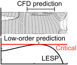
The main hypothesis in the current research is that the same critical value of LESP that governs LEV initiation on a 2-D airfoil also determines the time instant and spanwise location of LEV initiation on a finite wing. This hypothesis forms the basis of the low-order prediction of LEV initiation on a finite wing using UVLM. In this methodology, the spanwise variation of LESP along the wing, determined using UVLM, is calculated at each time instant during an unsteady motion. At the first time instant when the LESP value at any location on the span equals the critical LESP for the 2-D airfoil section (determined a priori using 2-D CFD or experiment), LEV initiation is assumed to occur on the wing. Additionally, the spanwise location corresponding to where the local LESP just equals the 2-D critical LESP is taken as the spanwise location of LEV initiation on the wing. Note that, the low-order prediction uses input only from 2-D CFD (or experiment), and does not use any information from the finite-wing CFD predictions. If the hypothesis is correct, the time instant, pitch angle and spanwise location of LEV initiation as predicted by the low-order UVLM method will agree closely with those predicted independently for the same wing and motion by the high-order (CFD) approach. In this subsection, the low-order prediction approach is illustrated for the baseline-wing case 1. Further, the hypothesis is tested by comparing the results from the low-order prediction for this case with those from the high-order results from § 3.5.3.
3.6.1. Low-order prediction illustrated using baseline-wing case 1
Figure 11 shows the spanwise distributions of LESP for three values of  $t^{*}$ for case 1. The LESP distribution is seen to grow with increasing
  $t^{*}$ because, for this range of
  $t^{*}$ values, the wing is undergoing a pitch-up motion. Also plotted in the figure is a red horizontal line which corresponds to the
  $\textrm {LESP}_{crit}$ of 0.27 for the SD7003 airfoil. A red error bar is included to denote the error in the
  $\textrm {LESP}_{crit}$ of 0.03, determined for this airfoil in § 3.5.2. It is seen that, at
  $t^{*}$ of 1.70, the maximum value of the UVLM-determined LESP distribution for the wing, which is at the wing root (at
  $y = 0$), just equals the 2-D
  $\textrm {LESP}_{crit}$ for the airfoil. Thus, using the hypothesis in § 3.6, the low-order prediction results in
  $t^{*}$ of 1.70 and
  $\alpha$ of
  $24.2^{\circ }$ for the LEV initiation for the baseline wing (case 1). These values compare excellently with the high-order predictions of
  $t^{*}$ of 1.71 and
  $\alpha$ of
  $24.4^{\circ }$ for this wing. Additionally, both methods predict that the spanwise location of LEV initiation corresponds to the wing root at
  $y = 0$. This excellent agreement shows that the low-order method is successful in predicting LEV initiation for the baseline-wing case 1, and verifies that the hypothesis of using 2-D
  $\textrm {LESP}_{crit}$ for low-order prediction of finite-wing LEV initiation has merit. In the following section, the hypothesis is further tested by comparing low-order and high-order predictions for all the remaining cases.

Figure 11. Spanwise variations of LESP from UVLM for three time instants for case 1, and  $\textrm {LESP}_{crit}$ from 2-D CFD for the SD7003 airfoil.
4. Results
The initiation of LEV formation for all the cases listed in table 1 were calculated using both the low-order and high-order prediction approaches. The major advantage of the low-order prediction approach is that it uses a fast analysis method (the UVLM) and a single value of  $\textrm {LESP}_{crit}$ obtained a priori from 2-D CFD or experiment (one for each airfoil used in the wing). Although we showed in § 3.6.1 that the low-order prediction of LEV initiation on the baseline wing (case 1) compared excellently with the high-order prediction, it is necessary to confirm if good agreement will also be seen for other wing geometries and motions.
The main objective of the study is to seek the answers to two key questions: (i) for each wing shape and motion, how well does the low-order prediction of time instant, pitch angle and spanwise location of LEV initiation agree with the high-order prediction? And (ii), how does LEV initiation vary with wing geometry and motion-kinematic parameters? With the aim of answering these questions, the results in this section are presented as eight case studies outlined in table 2. In each case study, case 1 is used as the baseline case for reference, and all the finite-wing results are compared with this case. For each case study, a single figure is used to compare the results from the high-order prediction with those from the low-order method. The high-order prediction for each wing will be presented as an upper-surface skin-friction plot at the instant of LEV initiation to show the  $t^{*}$,
  $\alpha$ and spanwise location of LEV initiation. Comparison of this plot with that for the baseline wing in figure 10(b) will enable the determination of how the LEV initiation differs from that for the baseline case. These comparisons for all the case studies will be used to answer the second of the two key questions. The low-order prediction will be presented as the spanwise distribution of LESP for the wing at the
  $t^{*}$ and
  $\alpha$ at which the LESP distribution first reaches the 2-D
  $\textrm {LESP}_{crit}$ value(s) for the airfoil(s) used in the wing. For comparison, this plot will also include the LESP distribution for the baseline case at LEV initiation, and horizontal lines to denote the 2-D
  $\textrm {LESP}_{crit}$ values for the airfoils. Comparison of the low-order predictions of
  $t^{*}$,
  $\alpha$ and spanwise location for LEV initiation with those predicted by the high-order method will enable assessment of the effectiveness of the low-order method, which will answer the first of the two key questions. Because the low-order method uses only the 2-D
  $\textrm {LESP}_{crit}$ for predicting the LEV initiation on the finite wing, good comparison between the low-order and high-order results for all the case studies will demonstrate that the same
  $\textrm {LESP}_{crit}$ value that governs LEV initiation on a 2-D airfoil also determines the time instant and spanwise location of LEV initiation on a finite wing.
Table 2. Case studies.

A summary of the results for all the cases is presented at the end of this section (in § 4.9) with two plots comparing low-order and high-order results for all the cases: the first plot comparing the pitch angle and the second plot comparing the spanwise location for LEV initiation. The discussion in § 4.9 also presents quantitative results to answer the two key questions posed earlier in this section. The numerical values for the  $t^{*}$,
  $\alpha$ and spanwise location of LEV initiation from the low-order and high-order predictions for all the wings are tabulated in the Appendix.
4.1. Case study A: effect of pivot location
In case study A, the initiation of the LEV for case 2 (pivot at  $x_{p}/c=0.75$) is compared with the baseline case (case 1, pivot at
  $x_{p}/c=0.25$) to study the effect of a change in pivot location. Figure 12 shows the comparison of results for the two pivot locations. The spanwise location for initiation of the LEV for case 2 (as deduced from the skin-friction plot in figure 12a) is similar to that for the baseline case 1 (figure 10b). The major difference from the baseline is that LEV initiation is delayed to a higher
  $t^{*}$ and
  $\alpha$ due to motion-induced ‘downwash’ at the leading edge. This trend of delayed LEV formation with aft movement of the pivot point is not new. The trend and the reasoning have been reported by several researchers including Ham & Garelick (Reference Ham and Garelick1968), Ericsson (Reference Ericsson1988), Visbal & Shang (Reference Visbal and Shang1989), Visbal & Gordnier (Reference Visbal and Gordnier1995), Ol (Reference Ol2009), Granlund, Ol & Bernal (Reference Granlund, Ol and Bernal2011) and Granlund et al. (Reference Granlund, Ol and Bernal2013).

Figure 12. Case study A: effect of pivot location. (a) CFD result for LEV initiation for case 2. (b) UVLM prediction for LEV initiation for case 2 compared with case 1.
In figure 12(b), the spanwise variation of LESP is shown to be nearly identical to that for the baseline. It is also seen that the low-order predictions for  $t^{*}$ and
  $\alpha$ for LEV initiation for case 2 agree well with the corresponding high-order predictions.
4.2. Case study B: effect of pitch rate
In case study B, the effect pitch rate on the initiation of the LEV is studied by comparing the results for cases 3 ( $K = 0.2$) and 4 (
 $K = 0.4$) with those for the baseline case (
 $K = 0.3$). The results for this case study are shown in figure 13. The upper-surface skin-friction lines, plotted in figure 13(a), show that the LEV initiation for these two cases starts at the wing root like for case 1. It is seen that, with increasing pitch rate, the chordwise extent of the trailing-edge reversed-flow region progressively reduces. There is a small increase in
  $\alpha$ for LEV initiation with increase in pitch rate. Increase in pitch rate increases the motion-induced downwash at the leading edge, causing the small delay in LEV initiation. This trend between the pitch rate and the time instant of LEV onset is consistent with the features and explanations in the literature: Ham & Garelick (Reference Ham and Garelick1968), Johnson & Ham (Reference Johnson and Ham1972), McCroskey, Carr & McAlister (Reference McCroskey, Carr and McAlister1976); McCroskey et al. (Reference McCroskey, McAlister, Carr, Pucci, Lambert and Indergrand1981), McCroskey & Pucci (Reference McCroskey and Pucci1982), Walker, Helin & Strickland (Reference Walker, Helin and Strickland1985), Carr (Reference Carr1988), Visbal & Shang (Reference Visbal and Shang1989), Acharya & Metwally (Reference Acharya and Metwally1992), Schreck & Helin (Reference Schreck and Helin1994), Ghosh Choudhuri & Knight (Reference Ghosh Choudhuri and Knight1996), Lian (Reference Lian2009) and Jantzen et al. (Reference Jantzen, Taira, Granlund and Ol2014).

Figure 13. Case study B: effect of pitch rate. (a) CFD results for LEV initiation for cases 3 and 4. (b) UVLM predictions for LEV initiation for cases 3 and 4 compared with case 1.
Figure 13(b) shows the low-order predictions for the spanwise LESP distributions at LEV initiation for cases 3 and 4, which reach the 2-D  $\textrm {LESP}_{crit}$ value at the wing root, indicating that the LEV initiation starts at the wing root. The low-order predictions for the
  $t^{*}$ and
  $\alpha$ for LEV initiation are in reasonable agreement (within
  $1.6^{\circ }$ for
  $\alpha$) with the corresponding high-order predictions.
4.3. Case study C: effect of taper ratio
In case study C, the initiation of the LEV for the tapered wing of case 5 (taper ratio of 0.5) is compared with that for the baseline case (taper ratio of 1). From figure 14(a), it is seen that the CFD-predicted LEV initiation for case 5 starts at approximately  $2y/b = 0.34$, which is similar to the observation of Spentzos et al. (Reference Spentzos, Barakos, Badcock, Richards, Coton and Galbraith2007) that LEV initiation on a tapered wing occurs between the wing root and tip (i.e. in the region
  $0 < 2y/b < 1$). Figure 14(b) compares the spanwise LESP distribution for case 5 with that for case 1. In contrast to the results for case 1, the spanwise LESP distribution for the tapered wing has a maximum near
  $2y/b = 0.32$, which agrees well with the CFD-predicted spanwise location for LEV initiation. The
  $t^{*}$ and
  $\alpha$ values for this low-order prediction also agree excellently with those from the high-order prediction.

Figure 14. Case study C: effect of taper ratio. (a) CFD result for LEV initiation for case 5. (b) UVLM prediction for LEV initiation for case 5 compared with case 1.
4.4. Case study D: effect of tip twist
In case study D, the initiation of the LEV for the twisted wing with 10° tip twist (case 6) is compared with the results for case 1 (no tip twist). The twisted wing in case 6 has a linearly increasing section incidence angle from root to tip. The upper portion of figure 15 shows that the LEV starts forming for this wing from  $2y/b$ of approximately 0.6. As seen from figure 15(b), the UVLM-predicted spanwise LESP distribution of case 6 has a clear maximum around the spanwise location of
  $2y/b$ of 0.6, which agrees excellently with the CFD prediction. The UVLM-predicted values for
  $t^{*}$ and
  $\alpha$ for LEV initiation also agree excellently with the CFD prediction. It is also seen that the
  $\alpha$ for LEV initiation for case 6 is approximately 5° less than that for case 1. This early initiation of the LEV formation is the result of higher incidence of the outboard sections due to tip twist.

Figure 15. Case study D: effect of tip twist. (a) CFD result for LEV initiation for case 6. (b) UVLM prediction for LEV initiation for case 6 compared with case 1.
4.5. Case study E: effect of AR
In case study E, the initiation of the LEV for the rectangular wing cases 7, 8 and 9 ( $AR=2$, 4, 8, respectively) are compared with that for the baseline case (case 1, rectangular wing of
  $AR=6$).
The AR effects on LEV initiation are presented in figure 16. Panel (a) shows the skin-friction plots for the rectangular wings with  $AR = 2$, 4 and 8, respectively. These three plots indicate that the onset location of LEV initiation is at the wing root for all these wings. Also seen is that, although the region near the wing tip for each wing where the skin-friction lines are influenced by the tip vortex are roughly of the same size for these three wings, the fraction of the wing occupied by this region is clearly the largest for the
  $AR = 2$ wing. Thus it can be expected that the lower-AR wings will be more influenced by the tip-vortex effects. Figure 16(b) shows the spanwise distributions of LESP for the four cases:
  $AR = 2$, 4, 6 and 8. Each of the four cases has the maximum in LESP at the root, which agrees with the CFD-predicted root location for the onset of LEV formation for each wing. While the
  $t^{*}$ and
  $\alpha$ values for LEV initiation for the
  $AR = 4$, 6 and 8 wings agree excellently with corresponding predictions from the high-order approach, the
  $AR = 2$ wing has CFD prediction for LEV initiation occurring at lower
  $t^{*}$ and
  $\alpha$ compared to the corresponding UVLM predictions. This discrepancy can be attributed to the increased effect of the ‘lifted-up’ tip-vortex structure on the downwash at the leading edge for the
  $AR = 2$ case due to the proximity of the tip vortex to the wing root. Because the UVLM does not take the lifting-up of the tip vortex into consideration, and instead assumes an attached tip vortex, the UVLM-predicted
  $\alpha$ for LEV initiation on the
  $AR = 2$ wing differs from the CFD prediction by almost
  $2.6^{\circ }$.

Figure 16. Case study E: effect of AR. (a) CFD results for LEV initiation for cases 7, 8 and 9. (b) UVLM prediction for LEV initiation for cases 7, 8 and 9 compared with case 1.
To investigate the influence of the tip-vortex structure on the UVLM predictions, the UVLM code was used to study the  $AR = 2$ (case 7) and
  $AR = 6$ (case 1) wings using the ‘attached-tip-flow model, or ATFM’ (figure 2a) and the ‘separated-tip-flow model, or STFM’ (figure 2c) options. Figure 17 presents the results from this study. It is seen that the
  $t^{*}$ and
  $\alpha$ results for
  $AR = 6$ wing are mostly independent of the tip-flow model used. On the other hand, for the
  $AR = 2$ wing, the
  $t^{*}$ and
  $\alpha$ predicted by the UVLM have better agreement with the CFD predictions when the separated-tip-flow model is used than when the attached-tip-flow model is used. This trend confirms the hypothesis that, for very low AR wings, it is important to capture the effects of the ‘lifted-off’ tip-vortex structure for improved predictions from the UVLM.

Figure 17. Comparison of UVLM predictions from attached-tip-flow model (ATFM) and separated-tip-flow model (STFM) for cases 1 and 7.
4.6. Case study F: effect of sweep angle
In case study F, the initiation of the LEV for the 30° swept-wing case 10 is compared with the baseline case (case 1, 0° sweep). It is to be noted that the pivot point for the swept wing is at the quarter-chord location of the root section. The top portion of figure 18 shows the CFD-predicted skin-friction lines on the upper surface at LEV initiation. In contrast to the results for all the other wings, this swept-wing case exhibits LEV initiation that starts close to the wing tip, and at a very small  $\alpha$ of
  $2.8^{\circ }$. The likely reason for this behaviour is that a pitch-up motion about the root quarter-chord location causes a significant motion-induced upwash towards the wing tips, causing the leading edge near the wing tip to become critical even at an early stage of the motion. The lower portion of figure 18 compares the spanwise distributions of LESP at LEV initiation for the swept wing and the unswept wing. It is seen that the LESP distribution for the swept wing is distinctly different from that for the unswept wing; it has a clear maximum near
  $2y/b =$ 0.9, which shows that, like the high-order approach, the low-order approach also predicts LEV initiation very close to the wing tip. It is seen that the low-order prediction for
  $\alpha$ is a small value of
  $1.5^{\circ }$, which is within
  $1.3^{\circ }$ of the CFD-predicted
  $\alpha$. This discrepancy in the predicted
  $\alpha$ for LEV initiation between the two methods is higher than that for the other cases. One possible reason for this discrepancy is that, like with the
  $AR = 2$ wing, the LEV occurs very close to the tip vortex. Because the UVLM models the tip vortex using an ‘attached-tip-flow’ model (figure 2a), there is error in the predicted value of LESP near the wing tips. Another reason could be that spanwise pressure gradient or spanwise flow, which have both been discussed by other researchers in the context of LEV initiation (Lorber, Covino & Carta Reference Lorber, Covino and Carta1991; Ellington et al. Reference Ellington, van den Berg, Willmott and Thomas1996; Jones & Babinsky Reference Jones and Babinsky2011), could be causing the discrepancy.

Figure 18. Case study F: effect of sweep angle. (a) CFD result for LEV initiation for case 10. (b) UVLM prediction for LEV initiation for case 10 compared with case 1.
4.7. Case study G: effect of abrupt change in incidence
In case study G, the initiation of the LEV for case 11, for which the wing geometry has a 4° higher incidence over the inboard third of the span, is compared with that for case 1. The top portion of figure 19 shows the upper-surface skin-friction lines for case 11. This plot shows the abrupt change in sectional skin-friction lines at  $2y/b = 0.33$, which is clearly related to the incidence change. It is seen that the LEV initiation for case 11 starts at the wing root, which is also to be expected owing to the increased incidence in that region. The lower portion of figure 19 shows the spanwise distributions of LESP for case 11 and the baseline case. It is seen that case 11 has a distinctly higher LESP over the inboard portion of the wing, resulting the low-order prediction for LEV initiation to occur at the wing root. It is also seen that the low-order and high-order predictions for
  $\alpha$ for LEV initiation on case 11 agree well with each other, and that case 11 has LEV initiation occurring approximately
  $4^{\circ }$ earlier than case 1.

Figure 19. Case study G: partially deflected wing. (a) CFD result for LEV initiation for case 11. (b) UVLM prediction for LEV initiation for case 11 compared with case 1.
4.8. Case study H: partially sharpened wing
In case study H, the initiation of the LEV for case 12, in which the wing has a sharpened leading edge over the inboard third of the wing span, is compared with the baseline case 1. The upper-surface skin-friction lines for case 12, in figure 20(a), shows that the LEV initiation starts at the wing root at  $\alpha$ of
  $21.3^{\circ }$. Figure 20(b) compares the spanwise variation of LESP and
  $\textrm {LESP}_{crit}$ for case 12 with the spanwise LESP for the baseline. Because of the abrupt change in airfoil between the inboard and the outboard portions of the wing, the 2-D
  $\textrm {LESP}_{crit}$ value also changes from the value of
  $\textrm {LESP}_{crit} = 0.27$ for the SD7003 airfoil in the outboard portions to the value of
  $\textrm {LESP}_{crit} = 0.24$ for the sharpened SD7003 airfoil in the inboard portion. For case 12, an excellent agreement is seen between the low-order and high-order predictions for the
  $t^{*}$ and
  $\alpha$ for LEV initiation. In contrast with case study G in which the abrupt change in section incidence caused a sudden change in the spanwise variation of LESP, the abrupt change in leading-edge radius in this case study causes an abrupt change in LESP
 $_{crit}$. Thus, while both cases 11 and 12 have a roughly 3–4° earlier LEV initiation compared to the baseline case, the earlier LEV initiation is achieved in different ways.

Figure 20. Case study H: partially sharpened wing. (a) CFD result for LEV initiation for case 12. (b) UVLM prediction for LEV initiation for case 12 compared with case 1.
4.9. Summary
Figure 21 presents a comparison of low-order (UVLM) predictions for all the 12 finite-wing cases with the respective high-order (CFD) predictions. In figure 21(a), the  $\alpha$ values for LEV initiation from UVLM are plotted against the CFD predictions as symbols for the 12 cases. The 45° line is co-plotted to denote perfect correlation, with the thickness of the line chosen to denote the CFD output resolution in
  $\alpha$ of
  ${\rm \Delta} \alpha = 0.5^{\circ }$, which is due to the difference in
  $t^{*}$ of 0.01 between two successive time instants at which the skin-friction data are written out by the CFD code, an example of which is shown in figure 10. It is seen that the
  $\alpha$ for LEV initiation has a spread of almost
  $40^{\circ }$ varying from
  $2.8^{\circ }$ for case 10 to
  $41.4^{\circ }$ for case 2. This large spread shows that criticality of
  $\alpha$ is not a good indicator for LEV initiation, as it varies significantly from case to case. In contrast, when the low-order prediction is made using the 2-D
  $\textrm {LESP}_{crit}$ value, the UVLM-to-CFD difference in
  $\alpha$ for LEV initiation is seen to be very good for all the cases as the symbols are all close to the 45° line. Among the cases considered, case 7 (the
  $AR = 2$ wing) has the maximum value of this UVLM-to-CFD difference in
  $\alpha$ of
  $2.6^{\circ }$, which is a result of the use of the attached-tip-flow model in the UVLM for a case in which tip-vortex effects are especially strong. Most of the other cases have much smaller UVLM-to-CFD differences; for all the other cases, the root-mean-square difference in
  $\alpha$ is
  $0.9^{\circ }$ and the maximum difference is
  $1.6^{\circ }$. Figure 21(b) shows a plot of the low-order prediction of the spanwise location of LEV initiation against the corresponding high-order prediction, using symbols to denote the 12 cases. In this figure too, the 45° line is plotted to show perfect correlation. The typical spanwise width over which LEV initiation was observed in the CFD for the 12 cases is shown as a horizontal error bar in the figure. It is seen that, although the spread for the spanwise locations ranges from the wing root (
 $2y/b = 0$) to almost the wing tip (
 $2y/b = 1$), the UVLM predictions for all cases agree remarkably well with the corresponding CFD observations. These excellent correlations in (i)
  $\alpha$ for LEV initiation, with a highest UVLM-to-CFD difference in
  $\alpha$ of
  $2.6^{\circ }$ for cases that are spread over a range of
  $41.4^{\circ }$, and (ii) spanwise location with a highest UVLM-to-CFD difference in
  $2y/b$ of approximately 0.02 for cases that are spread over a range of
  $-0.87 < 2y/b < 0.87$ demonstrate the power of the LESP concept in predicting the LEV initiation on a range of finite-wing geometries using just the 2-D
  $\textrm {LESP}_{crit}$ values for the sections used in the wings along with a low-order method like the UVLM.

Figure 21. Comparison of low-order (UVLM) predictions with high-order (CFD) results for all the finite-wing cases. (a) Pitch angle at LEV initiation. (b) Spanwise location of LEV initiation.
Although not presented here, the UVLM is capable of predicting forces and moments on the wing, which, as shown in Hirato (Reference Hirato2016), agree well with CFD predictions in attached-flow conditions. Soon after the formation of an LEV or the occurrence of significant trailing-edge separation, the force predictions from the UVLM start to deviate from the CFD results.
5. Conclusions
This paper presents a study of the initiation of LEV formation on finite wings undergoing pitch-up motion. An important objective was to explore if criticality of leading-edge suction, which was shown in earlier work to be closely connected with LEV initiation on airfoils, would also determine LEV initiation on finite wings. A large set of wing cases undergoing pitching motion were studied using RANS CFD computations to determine the high-order predictions for pitch angle and spanwise location of LEV initiation. The same cases were also analysed using an unsteady vortex lattice method to determine the spanwise variation of the leading-edge suction parameter at every time step of the motion. The low-order prediction for LEV initiation is assumed to occur at the first time instant when the UVLM-predicted LESP value at any location on the span equals the critical LESP for the 2-D airfoil section (determined a priori using 2-D CFD or experiment). It was seen that the pitch angle and spanwise location for LEV initiation from the low-order prediction for all the finite-wing cases matched excellently with those obtained from the high-order predictions. For the 12 wing cases used in the paper, the maximum UVLM-to-CFD difference in pitch angle was  $2.6^{\circ }$ for cases having a spread of
  $41.4^{\circ }$ in the pitch angle for LEV initiation. This result shows that it is possible to predict initiation of LEV formation on finite wings using a low-order method like a UVLM along with value(s) for the critical LESP for the airfoil(s) determined from two-dimensional CFD or experiments. Further, the low-order predictions for the spanwise locations for LEV initiation also agreed excellently with the CFD predictions in all cases.
While further refinement of the study is needed to better model the tip-vortex flow on low-AR wings in the UVLM formulation, the current results clearly show that the flow physics for initiation of LEV formation on finite wings is governed by a criticality of the LESP. During any motion, when the LESP on any spanwise portion of the wing reaches the critical value for that airfoil, LEV formation is initiated at that location. This criticality condition could be used to turn on and off LEV shedding in low-order prediction methods for finite wings with rounded leading edges. The insight from this research could also be used for LEV flow control to postpone or hasten LEV formation on various portions of a wing by controlling the LESP or critical LESP values.
Acknowledgements
The authors wish to gratefully acknowledge the support of the US Air Force Office of Scientific Research through grant FA 9550-13-1-0179 and program manager Dr D. Smith. The authors thank S. Aggarwal for his early contribution to this work. The authors also thank Professor Rockwell and Cambridge University Press for permission to reproduce the PIV images from Yilmaz & Rockwell (Reference Yilmaz and Rockwell2012). This article is a revised version of AIAA paper 2015-0546.
Declaration of interests
The authors report no conflict of interest.
Appendix. Summary of high-order and low-order predictions for all the cases
This appendix lists the numerical values for the  $t^{*}$,
  $\alpha$, and
  $2y/b$ predictions from the high-order and low-order methods for all the 12 finite-wing cases in table 3. These data were used in figures 21(a) and 21(b).
Table 3. Summary of LEV-initiation predictions for all the cases.


