2.1. Generation of fully developed TBL

Experiments are performed in a closed-circuit wind tunnel at the Harbin Institute of Technology Shenzhen in China. The test section of the wind tunnel is 5.6 m long with a cross-section of 0.8 m × 1.0 m. The flow in the tunnel is generated through an axial fan driven by an electric motor, with a maximum power of 75 kW. The free-stream velocity U _∞ in the test section can be varied between 1.5 and 50 m s⁻¹, with a longitudinal turbulence intensity of less than 0.4 % at U _∞ = 2.4 m s⁻¹ where most of experiments are performed. A smooth Perspex flat plate of 4.8 m length, 0.78 m width and 0.015 m thick, with its leading edge rounded into an elliptic profile, is mounted in the test section (figure 1). Two spanwise-aligned arrays of M4 screws, separated longitudinally by 0.015 m and placed at 0.1 m downstream of the leading edge, trip the boundary layer. A 0.2 m long end plate, inclined by 12 °, is attached to the trailing edge of the plate to avoid flow separation from the leading edge (Qiao, Zhou & Wu Reference Qiao, Zhou and Wu2017). The streamwise pressure gradient is carefully adjusted through slightly inclining the flat plate to 0.005 Pa m⁻¹. Most measurements are performed at 3.2 m downstream of the leading edge. The major parameters of the TBL are given in table 1, including the TBL thickness δ, momentum thickness θ, shape factor H ₁₂, friction velocity u_τ (${\equiv} \sqrt {\overline {{\tau _w}} /\rho } $, where τ_w is the local WSS, ρ is the density of air and the overbar denotes time averaging), viscous length scale δ_ν = ν/u_τ (ν is the kinetic viscosity of air), time scale $t_{\nu}$ = δ_ν/u_τ, Re_θ and Re_τ based on θ and u_τ, respectively. Unless otherwise stated, the superscripts ‘+’ and ‘*’ in this paper denote normalization by the inner scales and outer scales in the absence of control, respectively. The coordinate system (x, y, z) is defined in figure 1, with the origin at the mid-point of the trailing edge of the actuators. The instantaneous velocities along the x, y and z directions are denoted by $U = \bar{U} + u$, $V = \bar{V} + v$ and $W = \bar{W} + w$, respectively, where u, v and w are the fluctuating components.

Figure 1. Schematic of the experimental set-up for the generation of a TBL (not to scale; dimensions in millimetres).

Table 1. Characteristic parameters of the uncontrolled TBL.

2.2. Plasma actuators

In the present experiments, the plasma-generated near-wall spanwise flow may interact with oncoming flow to form streamwise vortices (Jukes & Choi Reference Jukes and Choi2012, Reference Jukes and Choi2013), aiming to merge the streaks and suppress the streak instability. Three plasma-actuator configurations (i.e. A, B and C) are investigated, each with different lateral spacings between the upper electrodes of the actuators, number of electrodes and plasma discharge direction along the z-axis (figure 2). Configurations A and B generate counter-rotating LSSVs, with distinct downstream developments, such as the strength and separation between the LSSVs. On the other hand, configuration C generates co-rotating LSSVs.

Figure 2. Schematic of three DBD plasma-actuator configurations (not to scale; dimensions in millimetres) and the photographs of the actuators and their discharges. (a,d) Configuration A, (b,e) configuration B, (c,f) configuration C. Control parameters of plasma actuators in (d–f): E = 5.75 kV_p–p, f = 11 kHz.

The schematic of each plasma actuator is shown in figure 2. Each DBD plasma actuator consists of upper and lower electrodes separated by a dielectric panel made up of one layer of Mylar tape and one layer of Kapton tape, giving an overall thickness of approximately 0.23 mm (≈ 1.5δ_ν). The lower electrode is connected to the ground. The influence of the actuators on the flow is examined via a comparison between the hot-wire-measured mean and root-mean-square (r.m.s.) velocity profiles with and without the actuators on the wall. In the presence of actuators on the wall, the mean and r.m.s. velocity profiles deviate from their counterparts without actuators by less than 1.0 %. This deviation is ascribed to the uncertainty (1.0 %) of the hot-wire measurements. A near-wall flow is generated from the upper to the lower electrode using a sinusoidal alternating current (AC) waveform applied with a voltage E = 3.50–6.75 kV_p–p (subscript p-p denotes peak-to-peak). Following Wang et al. (Reference Wang, Wong, Lu, Wu and Zhou2017) and Wong et al. (Reference Wong, Wang, Ma and Zhou2020), the frequency of E is fixed at 11 kHz, which is the optimum operating frequency of the power supply. The plasma discharge occurs at the long edge of the upper electrode and extends to the lower electrode in the z-direction depending on the magnitude of E. Figure 2(d–f) shows an example of discharge for the three configurations at E = 5.75 kV_p–p. The plasma discharge is captured with a digital camera placed in the wall-normal direction. The upper and lower electrodes are marked as grey and yellow rectangles, respectively. The total streamwise length of the actuator array is 240 mm (1600δ_ν), and its effective length (excluding a length of 20 mm or 133δ_ν at each end for wire connection) is 200 mm (1333δ_ν). The discharge, shown in purple colour, has a streamwise length of 200 mm (1333δ_ν).

For configuration A, each actuator consists of two upper and one lower electrodes (figure 2a). The separation between the two upper electrodes of an actuator is 100 wall units, the same as the mean spanwise separation between streaks. As such, six actuators cover the spanwise extent of the FE. The lower electrode in each actuator is positioned between two upper electrodes, thus generating plasma discharge in opposite directions. These actuators produce adjacent counter-rotating LSSVs, seen in the PIV data. Configuration B includes six actuators, each consisting of one upper and one lower electrode. The total number of the upper electrodes or the ‘total’ discharge length is halved compared with configuration A. The separation between the upper electrodes of two adjacent actuators or one pair of actuators, as illustrated in figure 2(b), is 60 mm or 400 wall units. The corresponding lower electrodes are positioned such that the two actuators generate plasma discharges in opposite directions, resulting in non-colliding counter-rotating LSSVs. Five actuators (figure 2c) are used in configuration C, and each consists of one upper and one lower electrode, producing plasma discharge in the same direction along the z-axis. The separation between the upper electrodes of two adjacent actuators is 267 wall units. Configuration C generates co-rotating LSSVs.

The total power consumption is estimated from voltage E and current I for each configuration. The value of I is measured across a non-inductive resistor (100 $\Omega$) connected in series between the lower electrode and the earth.

2.3. Hot-wire measurement

A single, constant temperature hot-wire of 5 μm (0.033δ_ν) in diameter and approximately 1.25 mm (8.3δ_ν) in length is mounted on a computer-controlled traversing system to measure the streamwise velocity across the TBL. The spatial resolution of the traversing system is 3.125 μm (0.021δ_ν) in the wall-normal direction. A total of 13 measurement points, with an increment of 50 μm (0.33δ_ν), are taken in the near-wall region to estimate the velocity gradient in the viscous sublayer. The longitudinal distance between the hot-wire and the trailing edge of the plasma actuators is 25 mm (167δ_ν) or more, well exceeding the critical separation (15 mm) suggested by Choi et al. (Reference Choi, Jukes and Whalley2011), to avoid destructive arcing (Choi et al. Reference Choi, Jukes and Whalley2011). Tests have been conducted to measure the hot-wire signals at x = 25 mm in the absence of incident flow, with and without plasma discharge. There is no appreciable difference in $\bar{U}$ observed between the two cases, suggesting a negligible effect of the plasma discharge on the hot-wire measurements. As the high-voltage power supply (CTP-2000 K) for generating the plasma produces an electronic noise of around 1.10 kHz, the sampling rate for the acquisition of the hot-wire data is chosen to be 3 kHz, with a cutoff frequency of 1 kHz. The sampling duration for each point is 40 s (28000 $t_{\nu}$), adequately long for the convergence, to within 1 % uncertainty, of the mean and r.m.s. values of the velocity. The hot-wire is calibrated with a Pitot tube connected to a micro-manometer (FCO510, with an accuracy of 0.25 % of the pressure reading and 0.001 Pa resolution). The same Pitot tube and the micro-manometer are used to measure the streamwise pressure gradient along the flat plate, as well as the pressure difference between the upper and lower sides of the floating element (FE) in the force balance measurements. Following Hutchins & Choi (Reference Hutchins and Choi2002), the first wall-normal position y ₀ of the hot-wire probe is obtained from linear fitting to $\bar{U}$ in the viscous sublayer. The fitting curve in the linear region can be written in the form of $\bar{U} = a{y_{ref}} + b$, where a and b are constants determined from fitting the equation to the measured data points, and y_ref is the wall-normal position away from the first hot-wire measurement point. Letting $\bar{U}\; = 0$ yields y_ref = −b/a or y ₀ = b/a.

2.4. PIV and smoke-wire flow visualization

A LaVision time-resolved PIV system is used to measure the flow structure, generated by plasma actuators, and the manipulated TBL in three orthogonal planes, i.e. the y–z, x–z and x–y planes. The flow is seeded with fog, with an average particle size of 1 μm, generated from peanut oil by a TSI 9307-6 particle generator. The flow is illuminated by 1.2 mm (8δ_ν) thick laser sheets shining through the side window, produced by a dual beam laser system (Litron LDY304-PIV, Nd: YLF, with a maximum energy output of 30 mJ per pulse) in conjunction with spherical and cylindrical lenses. For measurements in the y–z planes, one high-quality mirror of 80 mm × 150 mm is fixed on the plate at x = 0.51 m, 45 ° with respect to the y–z plane, downstream of the plasma actuator so that the images in the plane could be captured by a high-speed camera (Imager pro HS4M, 4-megapixel sensors, 2016 × 2016 pixels resolution) placed outside the working section. The image covers an area of 108 × 108 mm. For measurements in the x–z plane, the laser sheet shines through the plane of y ⁺ = 24. For measurements in the x–y planes, the laser sheet shines through the planes of z ⁺ = 0, 133 and 183. The image is captured by the same camera with a sampling frequency of 200 Hz. The total number of images captured is 1500 pairs for measurements in the y–z or x–z plane with a sampling frequency of 300 Hz. This number is increased to 2700 for measurements in the x–y plane to ensure the convergence of the dissipation and production of turbulent kinetic energy (TKE) to less than 1.5 %. In the image processing, the spatial cross-correlation, with an interrogation window of 32 × 32 pixels and a 50 % overlap along both directions of the image, determines the velocity vectors – a total of 15 876. The same number of vorticity data is obtained. The resulting spatial resolution is 0.9, 1.6 and 0.5 mm, or 6.0, 10.7, and 3.3 wall units for the y–z, x–z and x–y planes, respectively. The same PIV system is used for smoke-wire flow visualization experiments conducted in two x–z planes at y ⁺ = 20 and 50 with and without control. The value of U_∞ is set at 1.8 m s⁻¹ in order to ensure high quality flow visualization images. The smoke-wire is placed at y ⁺ = 17 or 47, and 150 mm (1000 wall units) downstream of the leading edge of the plasma actuators, parallel to the wall and normal to the free stream. The flow images are captured at 200 frames per second.

2.5. The μ-particle tracking velocimetry measurement

A μ-particle tracking velocimetry (μ-PTV) technique is deployed to measure the streamwise velocity near the wall, hence to measure the local WSS at U_∞ = 2.4–5.0 m s⁻¹, which will be used to calibrate the FE balance. The same camera as used in the PIV measurements is fitted with a long-distance microscope lens (Model K2) and two zoom lenses with a magnification factor of 2 so that the field of view is as small as 6.1 mm × 6.1 mm in the x–y plane (figure 4). As such, the spatial resolution reaches as high as 330 pixels mm⁻¹ – adequate for our need. Due to a large loss of the light intensity through the long-distance microscope lens, the μ-PTV measurement requires a much more powerful laser than the PIV measurement. A low-frequency laser source (Vlite-200), with a power of 200 mJ per pulse, is used to illuminate the flow field. The flow is seeded with particles of Di-Ethyl-Hexyl-Sebacat, with an average diameter of 1 μm, generated by a commercial particle generator (TSI 9307-6). The time interval between the two frames of an image pair is 40–75 μs (0.053–0.091 $t_{\nu}$), depending on U_∞. A total of 10 000 image pairs are captured, sampled at 15 Hz for each U_∞. The μ-PTV data are processed by an in-house developed algorithm. More details on this algorithm are given by Li et al. (Reference Li, Jessen, Roggenkamp, Klaas, Silex, Schiek and Schröder2015, Reference Li, Roggenkamp, Jessen, Klaas and Schröder2017). A spatial bypass filter is used to subtract the background of the images so that the centroid of each particle can be identified and tracked. As a result, the displacement of each particle and hence its velocity is easily computed. The captured flow field is divided into small strips parallel to the wall, with a height of 10 μm or 0.067–0.127 wall units depending on U_∞. The velocity vectors averaged within a strip to give the mean velocity. The local time-averaged WSS can then be calculated from the mean velocity gradient in the wall-normal direction in the viscous sublayer. Following Benedict & Gould (Reference Benedict and Gould1996) and Li et al. (Reference Li, Roggenkamp, Jessen, Klaas and Schröder2017), the variance of the mean streamwise velocity $\bar{U}$ may be written as $\textrm{var}(\bar{U}) = \overline {{u^2}} /N$, where N is the number of samples. Then, the theoretical sampling error of $\bar{U}$ with a 95 % confidence interval is given by $\Delta U = 1.96\sqrt {\textrm{var}(\bar{U})} $. This error is less than 0.8 % at U_∞ = 2.4–5 m s⁻¹ for the present μ-PTV measurements. Figure 3 presents the distributions of the mean streamwise velocity near the wall measured using both μ-PTV and hot-wire at U_∞ = 2.4 m s⁻¹ where the DR measurements are conducted. The inner-scale normalized streamwise velocity follows $\overline {{U^ + }} = {y^ + }$ at 2.5 < y ⁺ < 5, by both μ-PTV and hot-wire measurements. The departure of the hot-wire-measured WSS is less than 2 % of the μ-PTV data. This comparison provides a validation for the hot-wire measurements.

Figure 3. Comparison of the hot-wire- and μ-PTV-measured time-averaged streamwise velocities $\overline {{U^ + }} $.

Figure 4. Schematic of the FE balance and μ-PTV arrangement (not to scale; dimensions in mm). (1) Rectangular FE, (2) vertical beam, (3) horizontal steel rod, (4) counter-weight, (5) knife edge, (6) load cell.

2.6. Direct skin-friction measurement

It is a challenge to measure directly the skin-friction drag of a low Re_θ TBL, especially to resolve the variation of this force under control. The drag on the FE is presently of the order of 10⁻⁴ N, which is much smaller than that (10⁻²–10⁻¹ N) in Corke & Thomas (Reference Corke and Thomas2018) and Thomas et al. (Reference Thomas, Corke, Duong, Midya and Yates2019). A FE balance, schematically shown in figure 4, was built in house to measure this drag on a FE of area A = 0.1 × 0.2 m² whose leading edge is 15 mm (100 wall units) downstream of the trailing edge of the actuators (figure 1). The balance comprises of 6 main parts: (1) a rectangular FE of 0.2 m in spanwise width and 0.1 m in longitudinal length, (2) a vertical beam of length × width × thickness = 0.41 × 0.07 × 0.006 m, (3) a horizontal steel rod of 0.465 m in length and 0.012 m in diameter, (4) two counter-weights (12.5 and 25 g installed at the front and rear ends of the rod, respectively), (5) a knife edge, and (6) a force load cell (Honeywell M34, range ±50 g). The FE (1) is mounted on the vertical beam (2) which sits on the knife edge (5).

The FE balance follows the concept of Krogstad & Efros (Reference Krogstad and Efros2010), who managed to measure the WSS of the order of 10⁻¹ N in a rough-wall TBL. However, the present WSS on a smooth wall is much smaller, of the order of 10⁻⁴ N. As such, a series of improvements have been made to improve the resolution and minimize the measurement errors. Firstly, the balance works on the lever principle, and the horizontal drag force on the FE is amplified 45 times (nine times larger than that in Krogstad & Efros Reference Krogstad and Efros2010). The force amplification depends on the length of the vertical beam and the separation between the knife edge and the load cell. The vertical beam is made of aluminium alloy for high stiffness (90 N mm⁻²) with light weight (230 g). A relatively heavy and long horizontal steel rod (3) is used to damp out any FE vibration. The movement of the upper end of the beam is less than 1.5 μm, at U_∞ = 0–5.0 m s⁻¹; that is, the FE effectively does not rotate. Secondly, the amplified force pivoted about the knife edge is measured using a load cell, rather than a commercial weighing scale as used by Krogstad & Efros (Reference Krogstad and Efros2010), installed at 9 mm away from the knife-edged support perpendicular to the horizontal axis. The two counter-weights (4) act to preload the load cell to ensure its operation in the linear range. The load cell provides a more stable signal and captures the normal force only, with a resolution of 7.5 × 10⁻⁴ N. Amplified 45 times, the skin friction captured by the balance can be as small as 1.7 × 10⁻⁵ N. The force signal is offset, amplified and sampled at 1 kHz for the duration of 30 s using an National Instruments (NI) data acquisition system. Thirdly, as the flow outside the wind tunnel under the FE can greatly influence the force measurements (Baars et al. Reference Baars, Squire, Talluru, Abbassi, Hutchins and Marusic2016), the FE balance is housed in a sealed transparent Perspex box. The box is pressurized to that within the test section. Fourthly, the gap between the FE and the flat plate is only 0.5 mm. The FE-to-plate misalignment is measured using a high-resolution laser displacement sensor (OPTEX CD33) with a resolution of 7.5 μm. As shown in the inset of figure 4, this sensor, mounted on a three-dimensional traversing system with a spatial resolution of 3.125 μm, moves horizontally from the surrounding plate to the FE. The misalignment, determined from the distance between the two wall surfaces, is kept less than 7.5 μm by carefully adjusting the height of the adjustable feet (figure 4). Therefore, the gap-induced error is less than 1 % (Allen Reference Allen1977). Finally, the experimental set-up is carefully adjusted to ensure a streamwise pressure gradient of less than 0.005 Pa/m, and the FE is chosen to be 1 mm in thickness to minimize the difference between the static pressures on its leading and trailing edges. As a result, the error from the pressure gradient is reduced to less than 0.04 %. With these measures implemented, the balance is found to be able to capture reliably a skin-friction force of the order of 10⁻⁴ N.

The calibration of the present balance is another challenge. The conventional pulley system could not be used since the friction force between the wire and pulley is of the same order as the skin-friction drag. A novel and reliable calibration method is proposed. It has been confirmed that the μ-PTV-measured u_τ varies less than 1 % from the leading edge of the FE to the trailing edge. Furthermore, the flow is statistically two-dimensional in the absence of control. As such, the measured u_τ at the centre of the FE is taken as the mean value over the FE. This prompts us to determine the skin-friction force F on the FE over U_∞ = 0–5 m s⁻¹, which provides a calibration for the output voltage E_output. As shown in figure 5, the μ-PTV-measured mean streamwise velocity follows a linear variation near the wall, with an appreciable departure from the linearity only for y ⁺ > 5 for the U_∞ range examined. The local $\overline {{\tau _w}} $ is calculated from the velocity gradient in the viscous sublayer through

(2.1)\begin{equation}\overline {{\tau _w}} = \mu \frac{{\textrm{d}\bar{U}}}{{\textrm{d}y}}\quad \textrm{for}\;{y^ + } \le \textrm{ }5,\end{equation}

where μ (= ρν) is the dynamic viscosity of air. The uncertainty of $\overline {{\tau _w}} $ is analysed following Hutchins & Choi (Reference Hutchins and Choi2002). We calculate $\textrm{d}\bar{U}/\textrm{d}y$ by

(2.2)\begin{equation}\textrm{d}\bar{U}/\textrm{d}y = \frac{{\sum\limits_{i = 1}^n {({y_i} - {{\langle y\rangle }_n})(\overline {{U_i}} - {{\langle \bar{U}\rangle }_n})} }}{{\sum\limits_{i = 1}^n {{{({y_i} - {{\langle y\rangle }_n})}^2}} }},\end{equation}

where n is the number of points used to calculate $\textrm{d}\bar{U}/\textrm{d}y$, ranging from 15 to 32 depending on U_∞, and ${\langle \,\rangle _n}$ represents the average over n points. Then the standard error of $\overline {{\tau _w}} $, due to the least-squares fitting and velocity measurement uncertainty, is

(2.3)\begin{gather}\textrm{S}\textrm{.E}\textrm{.}(\overline {{\tau _w}} ) = \frac{{\mu {\sigma _u}}}{{{{\left[ {{{\sum\limits_{i = 1}^n {({y_i} - \bar{y})} }^2}} \right]}^{1/2}}}},\end{gather}

(2.4)\begin{gather}\sigma _u^2 = \frac{{\sum\limits_{i = 1}^n {{{(\overline {{U_i}} - {{\langle \bar{U}\rangle }_n})}^2}} - (\textrm{d}\bar{U}/\textrm{d}y)\sum\limits_{i = 1}^n {({y_i} - \bar{y})(\overline {{U_i}} - {{\langle \bar{U}\rangle }_n})} }}{{n - 2}}.\end{gather}

The uncertainty of $\overline {{\tau _w}} $ or $\textrm{S}\textrm{.E}\textrm{.}(\;\overline {{\tau _w}} )/\;\overline {{\tau _w}} $ is below 0.6 % over the range of U_∞ examined (figure 5). Then the skin-friction drag force F is approximated as

(2.5)\begin{equation}F = \overline {{\tau _w}} A = \rho u_\tau ^2A.\end{equation}

Figure 5. Wall-normal distributions of μ-PTV-measured mean streamwise velocity in the near-wall region normalized by (a) inner scales and (b) outer scales.

As shown in figure 6, E_output and F are linearly related. The maximum deviation between the data points and the fitting curve is 1.2 % for the entire calibration range.

Figure 6. Calibration curve of the FE-force balance, where $F = \rho u_\tau ^2A$ (u_τ is determined from the μ-PTV-measured streamwise velocity gradient measured at the centre of the FE) and E_output are the skin-friction drag on the FE and the output voltage of the balance, respectively. The error bars in red colour denote the standard deviation of the output voltage for 6-time repeated measurements.

The skin-friction coefficient c_f, defined as

(2.6)\begin{equation}{c_f} = \frac{{F/A}}{{0.5\rho U_\infty ^2}},\end{equation}

is presented in figure 7. The deviation of the present data from the Coles–Fernholz relation (c_f = 2/[1/0.384 × ln(Re_θ) + 4.127]⁻²) (Nagib, Chauhan & Monkewitz Reference Nagib, Chauhan and Monkewitz2007) is less than 3.5 %, which provides us with additional confidence in the present FE-force balance.

Figure 7. Comparison of the skin-friction coefficient c_f measured using the force balance with the Coles–Fernholz relation.

3.1. TBL in the absence of control

It is important to ensure the generation of a fully developed TBL at the leading edge of the plasma actuators. The Reynolds number based on the streamwise distance Re_x ( = U_∞x/ν) between the leading edges of the flat plate and plasma actuators is 4.6 × 10⁵ without tripping. Once tripped, the distribution of the mean streamwise velocity $\overline {{U^ + }} $ (figure 8a) across the boundary layer measured at the leading edge (x ⁺ = −1333, z ⁺ = 0) and also downstream of the actuators (x ⁺ = 167, z ⁺ = 0) collapses well with the law of wall (Pope Reference Pope2001). The r.m.s. value $u_{rms}^ +$ of the fluctuating streamwise velocity agrees well with Schlatter et al.'s (Reference Schlatter, Örlü, Li, Brethouwer, Fransson, Johansson, Alfredsson and Henningson2009) DNS and De Graaff & Eaton's (Reference De Graaff and Eaton2000) experiments. The results indicate that the TBL is indeed fully developed at these locations.

Figure 8. Profiles of (a) mean streamwise velocity $\overline {{U^ + }} $ at the leading edge (x ⁺ = −1333, z ⁺ = 0) of actuators and the test location (x ⁺ = 167, z ⁺ = 0) and (b) r.m.s. value $u_{rms}^ +$ of the fluctuating component u.

3.2. Plasma-induced flow structure

For configuration A, one pair of counter-rotating LSSVs is generated downstream of each actuator, as is evident in the PIV images (figure 9a) captured at the trailing edge of the actuators, i.e. x ⁺ = 0, covering $- 300 \le {z^ + } \le 300$. At E = 5.75 kV_p–p, the LSSVs collide with each other, forming strong upwash between the vortices generated by one actuator but downwash between adjacent actuators (figure 9a). The vortices within the same counter-rotating pair may be strengthened by their interactions (Lögdberg, Fransson & Alfredsson Reference Lögdberg, Fransson and Alfredsson2009) and progressively lifted away from the wall by mutual induction (Jukes & Choi Reference Jukes and Choi2012). Pauley & Eaton (Reference Pauley and Eaton1988) observed that counter-rotating streamwise vortices with common upflow lifted up while developing downstream. They proposed that the image vortices (Ersoy & Walker Reference Ersoy and Walker1985) in the wall caused the counter-rotating streamwise vortices to move towards each other and then move away from the wall. There are two consequences of this collision. First, the pair, as they come closer, become a strong vortex dipole and move away from the wall via mutual induction. Second, when pressed against each other, the two vortices undergo simultaneous weakening downstream because of the continual planar reconnection via cross-diffusion (Hussain & Duraisamy Reference Hussain and Duraisamy2011; Yao & Hussain Reference Yao and Hussain2020). Clearly, the actuators’ effect will thus decrease with increasing length due to mutual induction of adjacent LSSVs, discouraging the use of very long actuators. The optimum actuator length will depend on the spanwise spacing of the actuators, on the driving voltage which controls the strength of the wall jet and also on the local friction Reynolds number. These details are beyond the scope of the current paper and must await careful future studies. Note that due to the large separation between the two upper electrodes in configuration B, the counter-rotating LSSVs do not come close enough to each other and are not significantly altered by cross-diffusion (figure 9b). Furthermore, these LSSVs occur closer to the wall than in configuration A – this is to be expected because the two LSSVs of each pair are too far apart to be able to significantly move each when away from the wall via mutual interaction, and they are weakened much less as vorticity cross-diffusion is much lower. The inner-scale normalized circulation $ \varGamma^{+}$ of configuration B, calculated along the contour line of 10 % of the maximum vorticity, is 9.7, which is considerably smaller than that (15.8) for configuration A. This apparent contradiction can be reconciled by the fact that because the LSSVs remain closer to the wall in configuration B and thus undergo faster decay by higher viscous dissipation. Configuration C produces plasma discharge in the same direction along the z-axis, generating co-rotating LSSVs, as shown in figure 9(c). At E = 5.75 kV_p–p, the vortices are far away from the plasma discharge region of an actuator due to the unidirectional plasma-induced wall jet (Corke et al. Reference Corke, Enloe and Wilkinson2010), so that the LSSVs move along the same spanwise direction. The LSSVs are expected to decay slowly and to move laterally downstream (Jukes & Choi Reference Jukes and Choi2012) mainly by the mutual induction of the image vortices.

Figure 9. Time-averaged velocity vectors $(\overline {{V^ + }} ,\overline {{W^ + }} )$ and iso-contours of vorticity $\overline {\omega _x^ + } = \overline {\textrm{d}{V^ + }/\textrm{d}{z^ + }} - \overline {\textrm{d}{W^ + }/\textrm{d}{y^ + }} $ in the y–z plane at the trailing edge (x ⁺ = 0) of the plasma actuators. Configurations (a) A, (b) B and (c) C. The bold black contour denotes the level of 10 % of the maximum vorticity. The positive and negative electrodes are shown in black and red colours, respectively. Control parameter: E = 5.75 kV_p–p.

3.3. Dependence of DR on actuator configuration

Both FE-force balance and hot-wire are used to measure the DR downstream of the actuators, capturing the spatially averaged drag variation and the local drag variation along the spanwise and streamwise directions, respectively. The control performance is evaluated through the drag variation ΔF = (F_on − F_off)/F_off, where F_off and F_on are the skin friction on the FE without and with control, respectively. Note that the FE is mounted 15 mm downstream of the trailing edge of the actuators (figure 1). The ΔF depends on the E imposed as well as on the configuration, as shown in figure 10(a), where the error bars indicate the standard deviation of ΔF of six repeated measurements. Given the same E, the power consumption differs from each other between the configurations in figure 10(a) due to a difference in the number of electrodes and hence in the total ‘effective’ discharge length. In general, ΔF dips rapidly with increasing E for configurations A, B and C. Configuration B always corresponds to the smallest ΔF of all, and configuration A comes next in terms of the control performance. The LSSVs in configuration A may collide with each other as explained above, resulting in less DR than in B. Note that the larger separation between the LSSVs in B lengthens the wall jets, with corresponding weakening of their effectiveness (Yao et al. Reference Yao, Chen and Hussain2018). The maximum DR of both configurations A and B occurs at E = 5.75 kV_p–p, beyond which the drag recovers rapidly. The DR is connected to the plasma-generated vortices (figure 9). An increase in E increases the wall-jet velocity (Jukes et al. Reference Jukes, Choi, Johnson and Scott2006) and also the vortex strength, and hence a more pronounced drop in skin friction (Yao et al. Reference Yao, Chen and Hussain2018). However, beyond a certain level of E, say, at E > 5.75 kV_p–p, the vortices grow rapidly, causing an increase in vortex-induced shear stress or drag in the TBL (Schoppa & Hussain Reference Schoppa and Hussain1998; Iuso et al. Reference Iuso, Onorato, Spazzini and Di Cicca2002). A similar observation was made previously. Yao et al. (Reference Yao, Chen and Hussain2018) found from their DNS data that the skin-friction drag was reduced by the spanwise wall jet with the spanwise velocity low, but not high. They advocated that the spanwise wall jet suppresses the random turbulent shear stress associated with the QSVs in the TBL, while introducing additional coherent shear stress caused by the strong wall jets. With increasing E, the LSSVs are strengthened, shown later, and the coherent shear stress may exceed the reduction of the random shear stress, leading to a rise in drag. This is clear as with increasing wall-jet speed, the downwash also gets stronger, making the wall jet thinner and stronger and thus also increasing (dU/dy)_w (the subscript ‘w’ denotes the value on the wall) and hence the WSS (Jeong et al. Reference Jeong, Hussain, Schoppa and Kim1997).

Figure 10. (a) DR ΔF = (F_on − F_off)/F_off for configurations A, B and C, where F_on and F_off are the floating-element-balance-measured skin-friction drag with and without the plasma actuator operated, respectively. Here, E is the applied voltage. The error bars mark the standard deviation of the 6-time repeated results. (b) Variation of ΔF with the power input of three plasma-actuator configurations.

The DR of configuration C is always less than that of A or B. The maximum DR is only 10 % for configuration C, but approximately 20 % and 26 % for A and B, respectively. Unlike the opposed spanwise wall jets of configurations A and B, configuration C generates co-rotating LSSVs and the upwash induced by one vortex counters the downwash of the adjacent vortex. The counteraction could be avoided if the vortex spacing exceeds three times the vortex height (Jukes & Choi Reference Jukes and Choi2012). The spanwise spacing of the co-rotating LSSVs generated by plasma configuration C is 267 wall units, less than 3 times the vortex height (110 wall units). As a matter of fact, the interaction between two adjacent vortices is evident in the PIV-measured time-averaged velocity field (figure 9c), where the upwash of the right vortex counters the downwash of the left vortex. As a result, the strength of the vortices is the smallest among the three configurations. $ \varGamma^{+}$ in configuration C is only 7.9, which is appreciably smaller than in A and B. This interaction in the shear region may further lead to additional turbulence intensity (Pauley & Eaton Reference Pauley and Eaton1988). Consequently, the DR of configuration C is the smallest of the three. This is to be expected as the effective area of the intense wall jets is much less.

Figure 10(b) presents the relation between ΔF and the power consumption P_input where

(3.1)\begin{equation}{P_{input}} = \int_{{t_1}}^{{t_2}} {E(t)I(t)\,\textrm{d}t} .\end{equation}

In (3.1), E(t) and I(t) are the instantaneous voltage and current signals, and t ₁ and t ₂ are the starting and ending times of sampling, respectively. As P_input is correlated with the applied voltage, the DR variation with P_input is similar to that with E. Obviously, configurations A and B reach their maximum DR at the same voltage (E = 5.75 kV_p–p). However, the power consumption of configuration A is much larger than that of B, as the total discharge length of the former is two times more than that of the latter.

Figure 11 presents the control efficiency η = P_saved/P_input, where P_saved = (F_off − F_on) U _∞ is the time-averaged power saving due to plasma control, and P_input is the total energy input to manipulate the TBL. The power saved is several orders of magnitude smaller than the power consumed. Note that P_saved is calculated from the variation in drag on the FE and the actual power saving over the entire drag-reduced area will be much larger. Among the three configurations, the maximum η is achieved at E = 5.25 kV_p–p in B. The η of configuration B is in general largest of all (figure 11), outperforming other configurations in terms of the η as well as DR. As such, following discussion will focus on configuration B only.

Figure 11. Control efficiency $\eta = ({F_{off}} - {F_{on}}){U_\infty }/{P_{input}}$ for configurations A, B and C. Here, P_input is the power consumption, F_on and F_off are skin-friction drag acting on the FE with and without control, respectively.

3.4. Dependence of plasma-generated streamwise vorticity on applied voltage

For configuration B, the spatially averaged streamwise vorticity ${\langle \overline {{\omega _x}} \rangle _v}$ over the vortex enclosed by the contour of 10 % of the maximum vorticity is calculated from the PIV-measured time-averaged vorticity data in the y–z plane at the trailing edge (x ⁺ = 0) of the middle plasma-actuator pair. For E < 4.25 ${\rm kV}_{\rm p-p}$, ${\langle \overline {{\omega _x}} \rangle _v}$ scales linearly with E ^3.5 (figure 12) – similar to Wicks, Thomas & Corke's (Reference Wicks, Thomas, Corke, Patel and Cain2015) finding. However, when E > 4.25 kV_p–p, the rise in ${\langle \overline {{\omega _x}} \rangle _v}$ with E is slowed down and ${\langle \overline {{\omega _x}} \rangle _v} \propto {E^{1.6}}$. This variation with E exceeding a certain level is not unexpected. Thomas et al. (Reference Thomas, Corke, Iqbal, Kozlov and Schatzman2009) found that the plasma-generated body force was proportional to E ^3.5 at low voltages but to E ^2.3 at high voltages. With ${\langle \overline {{\omega _x}} \rangle _v}$ scaled with this body force (Wicks, Thomas & Corke Reference Wicks, Thomas, Corke, Patel and Cain2015), ${\langle \overline {{\omega _x}} \rangle _v}$ is expected to increase with E faster at low voltages but slower at high voltages. The difference between our and Thomas et al.'s (Reference Thomas, Corke, Iqbal, Kozlov and Schatzman2009) results may be due to a difference in the dielectric material or its thickness between the two studies. The dielectric panel is presently made of 0.073 mm thick Mylar tape and 0.055 mm thick Kapton tape but of a 6.35 mm thick Telfon sheet in Thomas et al. (Reference Thomas, Corke, Iqbal, Kozlov and Schatzman2009).

Figure 12. Spatial-averaged streamwise vorticity ${\langle \overline {{\omega _x}} \rangle _v}$ over the vortex enclosed by the contour of 10 % of the maximum vorticity. The value of ${\langle \overline {{\omega _x}} \rangle _v}$ is calculated from the PIV-measured time-averaged vorticity data in the y–z plane at the trailing edge (x ⁺ = 0) of the middle plasma-actuator pair. Here, E is the applied voltage (configuration B).

3.5. Relation between DR and maximum spanwise velocity

It is of interest to investigate the dependence of ΔF on wall-jet velocity. The maximum spanwise velocity $|\overline {{W_{max}}} {|^ + }$ in configuration B is calculated from the PIV-data in the y–z plane of x ⁺ = 0 (figure 13). The ΔF decreases with increasing $|\overline {{W_{max}}} {|^ + }$ until reaching its minimum at $|\overline {{W_{max}}} {|^ + } = 3.9$ and then increases. This is in good agreement with Yao et al.'s (Reference Yao, Chen, Thomas and Hussain2017, Reference Yao, Chen and Hussain2018) DNS data where the spanwise body force was introduced to generate the LSSVs in a channel flow, resulting in a DR of 19 %. Their best control performance was achieved when $|\overline {{W_{max}}} {|^ + }$ was approximately 4 times the friction velocity. They also proposed that the height of the maximum spanwise velocity $y_c^ +$ should be around 30 for the effective merger of numerous velocity streaks in the near-wall region, which is consistent with the present results at $y_c^ +{=} 24$ (figure 9b). They achieved a DR of only 1.4 % at a small $y_c^ +$ (= 5) since the wall jet was too thin to affect most parts of the streaks. So did they also at a large $y_c^ +$ (= 80). They explained that the smaller, secondary vortices between the primary vortices and the wall became strong at a large $y_c^ +$, leading to a stronger downwash which increases skin-friction drag.

Figure 13. Dependence of the FE-force-balance-measured drag change ΔF on the mean maximum spanwise velocity $|\overline {{W_{max}}} {|^ + }$ captured in the y–z plane (configuration B). The error bars denote the standard deviation of six repeats.

3.6. Local skin-friction drag variation

As the plasma actuators generate LSSVs (figure 9), the local friction variation cannot be expected to be uniform along the spanwise direction. The friction may further recover downstream. It is important to document how the local friction varies along the z- and x-directions, which is crucial for us to understand the flow physics behind DR.

The local DR is measured downstream of the plasma actuators for configuration B along the z- and x-directions, based on the hot-wire-measured gradient of the streamwise velocity in the sublayer. Since the actuators cannot withstand a high E for a long time, the hot-wire measurements are then performed at E = 4.25 kV_p–p and limited to only behind one half of the middle actuator pair, assuming a spanwise periodic variation in the DR. This assumption is reasonable because the two LSSVs generated by one pair of plasma actuators are statistically identical (figure 9). As such, the spanwise distribution of the local DR is expected to be symmetric about the centreline, i.e. z ⁺ = 0, between one pair of actuators and, for this reason, the data points are mirrored from the right to the left of z ⁺ = 0 (figure 14a), providing an overall view for the variation of DR. The local DR is measured at thirteen representative spanwise locations and ten streamwise positions, of which seven are over the FE and three are downstream of the FE. In figure 14, the local friction DR Δτ_w is given by $[{(\overline {{\tau _w}} )_{on}} - {(\overline {{\tau _w}} )_{off}}]/{(\overline {{\tau _w}} )_{off}}$, where ${(\overline {{\tau _w}} )_{on}}$ and ${(\overline {{\tau _w}} )_{off}}$ are the time-averaged WSS with and without plasma control, respectively, estimated from the streamwise velocity gradient in the sublayer.

Figure 14. (a) Spanwise distributions of the local DR Δτ_w at 10 streamwise locations. The solid symbols denote the hot-wire-measured points while the open symbols denote the symmetrized points to give a direct view of local DR distribution downstream from the middle actuator pair. (b) Streamwise distributions of Δτ_w at three representative locations, i.e. z ⁺ = 0, 133, 183. Configuration B: E = 4.25 kV_p–p. The red vertical dashed lines denote the locations of the PIV measurement Planes 4, 5 and 6 in figure 15.

Figure 14(a) shows that the spanwise distributions of Δτ_w are qualitatively the same for different streamwise locations and may be divided into three distinct regions – namely, the drag increase region (R1), the pronounced DR region (R2) and the drag recovery region (R3). In Region R2 (−160 < z ⁺ < −75 and 75 < z ⁺ < 160), the maximum DR is as high as 46 % at x ⁺ = 167, which corresponds spatially to the upwash of the LSSVs, as is evident in the PIV-measured time-averaged vorticity contours and velocity vectors in the y–z plane (Plane 4, figure 15). The low-speed fluid is lifted up from the wall, decreasing the streamwise velocity gradient near the wall, thus resulting in substantial DR. On the other hand, Region R1 occurs on the downwash side of the LSSVs, where the high-speed fluid is brought closer to the wall. The downwash of the high-speed fluid increases the streamwise velocity gradient near the wall and hence Δτ_w. Therefore, there is a significant drag increase, i.e. Δτ_w > 0, up to x ⁺ = 415 (figure 14b). These observations and inferences are consistent with those of Jeong et al. (Reference Jeong, Hussain, Schoppa and Kim1997) and Yao et al. (Reference Yao, Chen, Thomas and Hussain2017). Beyond x ⁺ = 415, the LSSVs become rather weak and shifted away from the wall (figure 15), and Δτ_w remains zero. Region R3 corresponds to an almost unchanged DR of approximately 23 % over −75 < z ⁺ < 75 at x ⁺ = 167. As will be seen later from flow visualization, the near-wall streaks in this region are stabilized as a result of the reduced meandering (Schoppa & Hussain Reference Schoppa and Hussain2002) which is modulated by the LSSVs. Similar spanwise distribution of local DR could also be found in the results of Iuso et al. (Reference Iuso, Onorato, Spazzini and Di Cicca2002) and Canton et al. (Reference Canton, Örlü, Chin, Hutchins, Monty and Schlatter2016a).

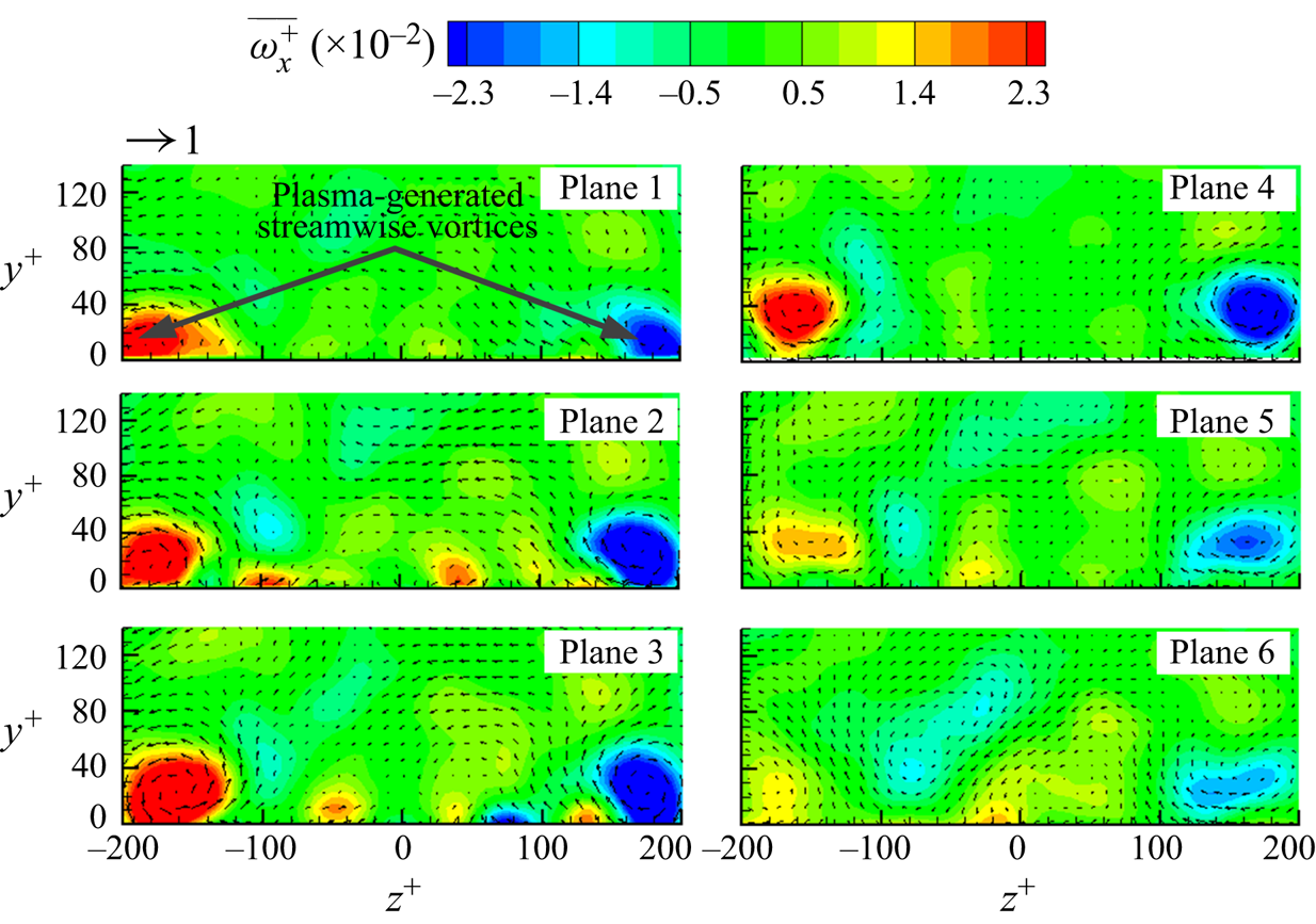
Figure 15. Time-averaged vorticity $\overline {\omega _x^ + } = \overline {\textrm{d}{V^ + }/\textrm{d}{z^ + }} - \overline {\textrm{d}{W^ + }/\textrm{d}{y^ + }} $ and velocity vectors $(\overline {{V^ + }} ,\overline {{W^ + }} )$ in the y–z planes at x ⁺ = −889, −444, 0, 167, 433, 767. Configuration B: E = 4.25 kV_p–p.

The streamwise recovery of Δτ_w is closely linked to the development of LSSVs, which (Plane 1 of figure 15) are generated right above the electrodes (figure 2b). These vortices grow in both strength and size when developing downstream from Plane 1 (x ⁺ = −889) to Plane 3 (x ⁺ = 0) due to the continually injected momentum by the plasma actuators, leading to a spatial evolution in the local DR over the actuators. This evolution, however, cannot be measured presently. Behind the actuators, the vortices grow very slowly in size but decay rapidly in strength, perhaps due to cross-diffusion as well as viscous dissipation. The observation is consistent with the streamwise recovery of Δτ_w. In figure 14(b), Δτ_w in Region R2 or R3 is initially pronouncedly negative and recovers gradually to the value of the natural state with increasing x ⁺, while Δτ_w measured in Region R1 drops from a level significantly positive to negative at x ⁺ = 415 and then maintains below zero before approaching the natural state. Note that Δτ_w does not overshoot, i.e. becoming positive, after reaching zero beyond x ⁺ = 2000. This is different from the drag recovery controlled by LSSVs in Iuso et al. (Reference Iuso, Onorato, Spazzini and Di Cicca2002), where additional mass was introduced into the flow.

The strength (quantified by the plasma-generated vorticity in the time-averaged PIV measurements) of LSSVs decays rapidly as shown in the Planes 3 to 6 of figure 15, while the drag recovers relatively slowly downstream to its natural state. At x ⁺ = 767, the maximum vorticity is negligibly small (Plane 6, figure 15), while the corresponding maximum local DR remains as high as 20 % at z ⁺ = 133. This indicates that the low-drag state may persist even after the LSSVs vanish, which is consistent with Schoppa & Hussain's (Reference Schoppa and Hussain1998) finding of the persistence of the low-drag state even upon sudden and complete termination of the spanwise control flow. Schoppa & Hussain (Reference Schoppa and Hussain1998) estimated the drag recovery distance of approximately 16 000 wall units by multiplying the relaxation time Δt ⁺ (in an order of 1000) of the controlled flow with the centreline flow velocity. If the same formula is used, the drag recovery distance would be $(U_\infty ^ + )(\mathrm{\Delta }{t^ + })\sim 23\,000$ wall units in our case, much larger than the presently observed 2000 wall units. Two factors may account for the difference. Firstly, the LSSVs induced are structurally different in wall-jet profiles between the two studies. The LSSVs in Schoppa & Hussain (Reference Schoppa and Hussain1998) collide with each other, with the maximum spanwise velocity at H/2 (H is the channel half-width), corresponding to approximately 80 wall units away from the wall. In contrast, the LSSVs generated by present configuration B do not collide and the maximum spanwise velocity occurs at y ⁺ = 24, implying a stronger interaction between the vortices and also with their image vortices (discussed earlier). Secondly, the real controlled flow may recover sooner than the estimation from $(U_\infty ^ + )(\mathrm{\Delta }{t^ + })$. Iuso et al. (Reference Iuso, Onorato, Spazzini and Di Cicca2002) experimentally introduced jet-induced LSSVs in a channel flow, and found a drag recovery distance of 9000 wall units, far less than that (~18 000 wall units) calculated from $(U_\infty ^ + )(\mathrm{\Delta }{t^ + })$, even with a large control jet velocity (100u_τ). The present spanwise velocity is less than u_τ, about 0.92 u_τ, at E = 4.25 kV_p–p (figure 13). Therefore, the difference may not be surprising.

The spanwise-averaged DR at each x ⁺ could be determined from spanwise integration of the hot-wire-measured local DR. The three pairs of plasma actuators in configuration B are identical (figure 16a). Note that the spanwise distribution of local Δτ_w downstream of the side actuator pair (z ⁺ = −800~−534 or 534–800) differs from that behind the middle (z ⁺ = 0–267). Obviously, the LSSVs behind the middle may interact on both sides with those generated by the adjacent actuator pairs. Those behind the left- or right-side actuator pair, however, interact only on one side with the LSSVs behind the middle pair. Indeed, as shown in figure 16(b), the distribution of Δτ_w behind the right-side actuator pair (z ⁺ = 534–800) exhibits a considerable difference from that behind the middle pair (z ⁺ = 0–267) at x ⁺ = 167 and 767, which correspond to the most upstream and most downstream locations of the hot-wire-measured Δτ_w data over the FE, respectively. The vertical pink dashed line denotes the spanwise position of the actuator edge at z ⁺ = 767. Evidently, Δτ_w is appreciably non-zero until z ⁺ ≈ 867 due to the stabilized streaks under the influence of the plasma-generated LSSVs. Nevertheless, the distribution of Δτ_w over z ⁺ = 533–716 (behind the right-side actuator pair) collapses completely with that over z ⁺ = 0–183 (behind the middle pair). That is, the distribution of Δτ_w in Area II is identical to that in Area I (figure 16a). Therefore, for $167 \le {x^ + } \le 767$, the distribution of Δτ_w downstream of the left- and right-side actuator pair over the FE area may be represented by that downstream of the middle actuator pair due to symmetry and periodicity. The spanwise-averaged drag change at a given streamwise location is then given by

(3.2)\begin{equation}{\langle \Delta {\tau _w}\rangle _z} = \frac{{\displaystyle\int_{z_1^ + }^{z_2^ + } {\Delta {\tau _w}\,\textrm{d}z} }}{{z_2^ +{-} z_1^ + }},\end{equation}

where ${\langle \,\rangle _z}$ denotes spanwise-averaging, $z_1^ +$ and $z_2^ +$ are −667 and 667, corresponding to the spanwise edges of the FE. Thus calculated ${\langle \Delta {\tau _w}\rangle _z}$ is presented in figure 17, along with $ - {|{\overline {{\omega_{xmax}}} } |^ + }$ and $-|\overline {{W_{max}}} {|^ + }$. The ${|{\overline {{\omega_{xmax}}} } |^ + }$ and $|\overline {{W_{max}}} {|^ + }$ values are the peaks of the streamwise vorticity and the spanwise velocity, respectively, in the time-averaged vorticity and velocity at x ⁺ = 0, 167, 433, 767 (Planes 3, 4, 5 and 6 in figure 15) out of 1500 PIV images. When appropriately scaled, the variations of ${|{\overline {{\omega_{xmax}}} } |^ + }$ and $|\overline {{W_{max}}} {|^ + }$ in x are quite similar to each other. Both $ - {|{\overline {{\omega_{xmax}}} } |^ + }$ and $ - |\overline {{W_{max}}} {|^ + }$ rise with increasing x ⁺ due to the decay of the LSSVs, which is closely correlated with the increasing ${\langle \Delta {\tau _w}\rangle _z}$. We estimate, based on this correlation (figure 17), ${\langle \Delta {\tau _w}\rangle _z}$ at x ⁺ = 0 (the trailing edge of the plasma actuators) to be −22 %, where the hot-wire measurement is not possible. The streamwise integration of ${\langle \Delta {\tau _w}\rangle _z}$ (figure 17) from x = 15 to 115 mm or x ⁺ = 100 to 767 yields the DR on the FE-force balance measurement area of 100 × 200 mm² or 667 × 1333 wall units, viz.

(3.3)\begin{equation}{\langle \Delta {\tau _w}\rangle _{xz}} = \frac{{\displaystyle\int_{x_1^ + }^{x_2^ + } {{{\langle \Delta {\tau _w}\rangle }_z}\,\textrm{d}x} }}{{x_2^ +{-} x_1^ + }},\end{equation}

where ${\langle \,\rangle _{xz}}$ denotes the spatial average along both z and x directions, and $x_1^ +$ and $x_2^ +$ are 100 and 767, respectively. The value of ${\langle \Delta {\tau _w}\rangle _{xz}}$ is found to be −12.0 % at E = 4.25 kV_p–p, whilst the FE-force balance-measured DR is −10.8 % (figure 10a). The difference in the DR between the hot-wire and force balance measurements may result from the experimental uncertainties of the two techniques. As shown in figure 10(a), the uncertainty of the force-balance-measured DR under f = 11 kHz, E = 4.25 kV_p–p is 1.6 %, which is larger than the difference (1.2 %) in the DR between the two measurements. Note that the spanwise-averaged DR drops along the streamwise direction, as shown figure 17, implying that the fully developed value of the DR at the trailing edge of the actuators, where the strength of the plasma-generated streamwise vortices is the maximum, would be larger than that measured by the FE-force balance.

Figure 16. (a) Schematic of hot-wire measurement locations over the FE area denoted by black and blue symbols. (b) Comparison between the spanwise distributions of hot-wire-measured local DR Δτ_w at x ⁺ = 167 and 767, behind the middle and side pairs of actuators. The vertical red and pink dashed lines at z ⁺ = 667 and 767 denote the spanwise edges of FE and the right-side actuator pair, respectively.

Figure 17. Variation of spanwise-averaged DR ${\langle \Delta {\tau _w}\rangle _z}$ (□), the negative maximum mean spanwise velocity $-|\overline {{W_{max}}} {|^ + }$ (Δ) and negative maximum mean streamwise vorticity $ - {|{\overline {{\omega_{xmax}}} } |^ + }$ (⋆) along the x ⁺ direction. Configuration B: E = 4.25 kV_p–p.

In order to estimate the ‘total’ DR downstream of the actuators, ${\langle \Delta {\tau _w}\rangle _z}$ is integrated from x ⁺ = 0 to 2000 (figure 17), yielding ${\langle \Delta {\tau _w}\rangle _{xz}} ={-} 7.12\%$. Note that the DR over the FE at E = 5.75 kV_p–p is 2.5 times that at E = 4.25 kV_p–p (figure 10a). For the same drag recovery rate, the DR area would be extended much larger than x ⁺ = 2000. Evidently, the DR area exceeds greatly that achieved by some other techniques. For instance, the drag recovers fully at x ⁺ = 160 for Bai et al.'s (Reference Bai, Zhou, Zhang, Xu, Wang and Antonia2014) wall-normal oscillation technique.

4.1. Mean and r.m.s. streamwise velocities

Mean streamwise velocity profiles normalized by both local inner and outer scales are presented in figure 18. In the absence of control, the $\overline {{U^ + }} $ profile collapses well with that reported by Ricco & Wu (Reference Ricco and Wu2004), showing a linear near-wall region for y ⁺ < 5 and a log region for 30 < y ⁺ < 170. Under control, the $\overline {{U^ + }} $ profile still follows $\overline {{U^ + }} = {y^ + }$ in the near-wall region, while the log region shifts upwards or downwards, depending on the local drag change. At z ⁺ = 133 (Region R2) and 0 (Region R3), where the local WSS is reduced, there is the expected upward shift of the log layer for increased DR (figure 18a,c). This is consistent with the results of Ricco & Wu (Reference Ricco and Wu2004), who experimentally investigated the spanwise wall oscillation in the TBL and achieved the maximum DR of 32 %. Note that the slope of the $\overline {{U^ + }}$ profile in the log-law region in Ricco & Wu (Reference Ricco and Wu2004) is identical to the uncontrolled flow, as the mean streamwise velocity is affected only for y ⁺ < 30 and the shift of the log region results directly from the reduced friction velocity used for normalization. A similar phenomenon is also observed in the present study at z ⁺ = 0. However, at z ⁺ = 133, corresponding to the maximum DR location, the slope of the $\overline {{U^ + }} $ profile increases compared with the uncontrolled flow due to the strong upwash of the LSSVs. On the other hand, at z ⁺ = 183 in Region R1, the local drag increases and the logarithmic region shows the expected downward shifts. The streamwise velocity profiles normalized by outer scales may give an intuitive view of the changes as the boundary layer thickness and the free-stream velocity are unchanged under control. There is a distinct deficit of $\bar{U}/{U_\infty }$ in the near-wall region at z ⁺ = 133 and 0 (the insets in figure 18d,f), which is consistent with the measured DR in these locations. In comparison, $\bar{U}/{U_\infty }$ at z ⁺ = 183 under control is larger than without control in the near-wall region. At z ⁺ = 133 where the largest DR is achieved, the strong upwash due to LSSVs may produce a change in $\bar{U}/{U_\infty }$ over y/δ = 0–0.29 (figure 18d). In other words, almost the entire log-law region is affected by the control, which accounts for the increased slope of the $\overline {{U^ + }} $ profile in the region (figure 18a). At the other two locations (z ⁺ = 0 and 183), the changes in the velocity profile are limited to y/δ < 0.04.

Figure 18. Mean streamwise velocity $\overline {{U^ + }} $ profiles in (a–c) inner and (d–f) outer scales (configuration B: E = 4.25 kV_p–p); (a,d) (x ⁺, z ⁺) = (167, 133), (b,e) (167, 183), (c,f) (167, 0). The insets in (d–f) are the zoom-in views of the near-wall region.

Figure 19 presents the u_rms profiles, normalized by both local inner and outer scales. At z ⁺ = 133 in Region R2, $u_{rms}^ +$ changes little for y ⁺ < 3 under control. However, $u_{rms}^ +$ increases rapidly, exceeding that of the uncontrolled flow, away from the wall until y ⁺ = 220, due to the perturbation by the LSSVs. Yao et al. (Reference Yao, Chen and Hussain2018) made a similar observation and attributed the increased $u_{rms}^ +$ to the advection of the externally introduced LSSVS, which could transport the near-wall turbulence and the QSVs to the outer flow. The movement of these structures is also reflected in the altered wall-normal location of $u_{rms}^ +$, which moves away from y ⁺ = 14 to 19. Tardu (Reference Tardu2001) proposed that DR be achievable by pushing the QSVs away from the wall or decreasing their intensity. The upward movement of the QSVs is consistent with the observed DR. Similar phenomenon is also found at z ⁺ = 0, albeit with smaller $u_{rms}^ +$. At z ⁺ = 183 in Region R1, $u_{rms}^ +$ is always smaller under control than without control for y ⁺ < 35, as noted by Canton et al. (Reference Canton, Örlü, Chin, Hutchins, Monty and Schlatter2016a) in their DNS data, where the spanwise body force was introduced to generate LSSVs in a turbulent channel. Note that at z ⁺ = 133 (figure 19a) the $u_{rms}^ +$ profile under control does not collapse with that in the natural flow for y ⁺ > 300, which is attributed to the normalization of y by the local wall variables (Bai et al. Reference Bai, Zhou, Zhang, Xu, Wang and Antonia2014), not to control. The y extent of control-affected region could be inferred in outer-scaled plot (figure 19d–f). At all three spanwise locations, u_rms/U_∞ with and without control collapse beyond 0.29δ. It is noteworthy that the variations of u_rms in outer scales are almost opposite to that in inner scales in the near-wall region. For example, although $u_{rms}^ +$ increases within 3 < y ⁺ < 12 at z ⁺ = 0 and 133 under control, u_rms is even lower than in the uncontrolled case (the insets in figure 19d,f) as a direct result of the lift up of the QSVs by the upwash effect of the LSSVs. Yet, the inner scales, i.e. u_τ and δ_ν, change considerably under control due to substantial local DR, causing an increase in $u_{rms}^ +$.

Figure 19. Profiles of the r.m.s. value of fluctuating velocity u normalized by their local (a–c) inner and (d–f) outer scales (configuration B: E = 4.25 kV_p–p); (a,d) (x ⁺, z ⁺) = (167, 133), (b,e) (167, 183), (c,f) (167, 0). The insets in (d–f) show the near-wall region.

4.2. Visualized flow structure

The flow structure modification under control is well captured by the smoke-wire flow visualization in two x-z planes at y ⁺ = 20 and 50, as shown in figures 20 and 21, respectively. Attempts were also made for y ⁺ < 20, though unsuccessful because the smoke-wire burned out easily due to the high voltage needed for plasma actuators. The value of U_∞ was chosen at 1.8 m s⁻¹ to capture the flow visualization images of good quality. At the height of y ⁺ = 20, smoke filaments originating from the smoke-wire, placed at y ⁺ = 17, rise and track the organized motions or QSVs, forming the low-speed streaks, and are illuminated by the x–z laser sheet at y ⁺ = 20. On the other hand, the high-speed fluid is swept by vortices, resulting in high-speed streaks, which contain no seeding particles to be illuminated by the laser sheet. In the absence of control, the low- and high-speed streaks take place side by side alternately, and they occur rather randomly in both space and time. The spanwise spacing between low-speed streaks is approximately 100δ_ν, which is consistent with the literature (e.g. Kline et al. Reference Kline, Reynolds, Schraub and Runstadler1967; Schoppa & Hussain Reference Schoppa and Hussain2002; Bai et al. Reference Bai, Zhou, Zhang, Xu, Wang and Antonia2014). Once the control is applied, the streaks change greatly, becoming more organized and stabilized due to the LSSVs, as shown in figure 20(b). The illuminated, white-coloured low-speed streaks are all pushed into the central region of each actuator pair by the wall jets. These streaks merge, forming a streak envelope. Meanwhile, the darker high-speed fluid lies between the low-speed streak envelopes due to the downwash of the LSSVs. A similar observation is made by Yao et al. (Reference Yao, Chen and Hussain2018) based on the DNS data in a channel flow, where many low-speed streaks merged under the influence of spanwise-opposed wall jets (Schoppa & Hussain Reference Schoppa and Hussain1998). The altered flow structures are in distinct contrast with those under the spanwise wall-oscillation control in Choi, Debisschop & Clayton (Reference Choi, Debisschop and Clayton1998) and Karniadakis & Choi (Reference Karniadakis and Choi2003). Under the spanwise wall oscillation, the natural streaky structures are tilted away from the mean flow direction at the leading edge of the oscillating plate. They proposed that the negative spanwise vorticity was generated during the spanwise wall oscillation and, as a result, the streamwise velocity in the near wall of the TBL was reduced, accounting for the friction DR.

Figure 20. Smoke-wire flow visualization of instantaneous flow structure in the x–z planes. (a) Uncontrolled; (b) under control (configuration B: E = 5.75 kV_p–p). The smoke-wire and the laser sheet are positioned at y ⁺ = 17 and 20, respectively. Flow at U _∞ = 1.8 m s⁻¹ is left to right. The red dashed lines indicate the centrelines of the actuator pairs. The horizontal blue-coloured bars and the vertical arrows represent the upper electrodes of the plasma actuators and the ionic wind direction, respectively.

Figure 21. Smoke-wire flow visualization of instantaneous flow structure in the x–z planes. (a) Uncontrolled; (b) under control. The smoke-wire and the laser sheet are positioned at y ⁺ = 47 and 50, respectively. Please refer to figure 20 for flow conditions and legends.

In the absence of control, the streaks in the plane of y ⁺ = 50 (figure 21) are more meandered and chaotic than those at y ⁺ = 20, due to the weak ejection and sweep motions in the lower part of the log region (Kline et al. Reference Kline, Reynolds, Schraub and Runstadler1967). Under control, the streaks are pushed toward the centreline of the actuator pairs, like the case at y ⁺ = 20, although exhibiting more meandering motions. The occurrence of the more meandering streaks results from upwash of QSVs by LSSVs, also producing increased $u_{rms}^ +$ in this region. From a different perspective, consider the turbulence regeneration cycle proposed by Kim (Reference Kim2011) and Schoppa & Hussain (Reference Schoppa and Hussain2002). The near-wall streaks are generated from the fluid lift-up by the QSVs (Jeong et al Reference Jeong, Hussain, Schoppa and Kim1997; Jimenez & Pinelli Reference Jimenez and Pinelli1999). These streaks are unstable to both the normal-mode instability (Hamilton, Kim & Waleffe Reference Hamilton, Kim and Waleffe1995) and particularly the non-normal-mode instability, namely, transient growth (Schoppa & Hussain Reference Schoppa and Hussain2002), resulting in the streamwise-dependent spanwise flow disturbances which are necessary to generate new QSVs. Using DNS, Schoppa & Hussain (Reference Schoppa and Hussain2002) demonstrated that the normal-mode streak instability could not cause significant vortex generation near the wall, due to a limited amplification (only twofold). They presented the streak transient growth mechanism, which is capable of producing much larger amplification (tenfold) of the x-dependent disturbances and accounts for the formation of a sheet of streamwise vorticity, which then leads to the generation of new QSVs via stretching by ∂u/∂x of the meandering streaks. In view of the stabilized streaks due to reduced streak flank angle under control, the generation of new QSVs is suppressed; therefore, the skin-friction drag is reduced significantly.

4.3. Suppressed wall-normal vorticity

A change in the streak transient growth is also reflected in the wall-normal vorticity ω_y because of the close association between this and ω_y (Schoppa & Hussain Reference Schoppa and Hussain2002; Kim Reference Kim2011). Figure 22 presents the probability density function (PDF) of ω_y/ω_yrms, calculated from the PIV data captured downstream of the plasma actuators in the x–z plane of y ⁺ = 24. The calculation area is the same as the area of the FE. Once plasma control is applied, the probability of large ω_y/ω_yrms drops appreciably compared to that in the uncontrolled flow, while that of small ω_y/ω_yrms is significantly increased, indicating a decreased ω_y over the FE area. A similar result was also obtained by Iuso et al. (Reference Iuso, Onorato, Spazzini and Di Cicca2002), who achieved a spanwise-averaged DR of 15 % in a turbulent channel flow using an array of inclined wall jets to induce LSSVs. The observed change in ω_y/ω_yrms implies stabilized streaks and the suppressed transient growth leading to fewer QSVs, hence the observed DR.

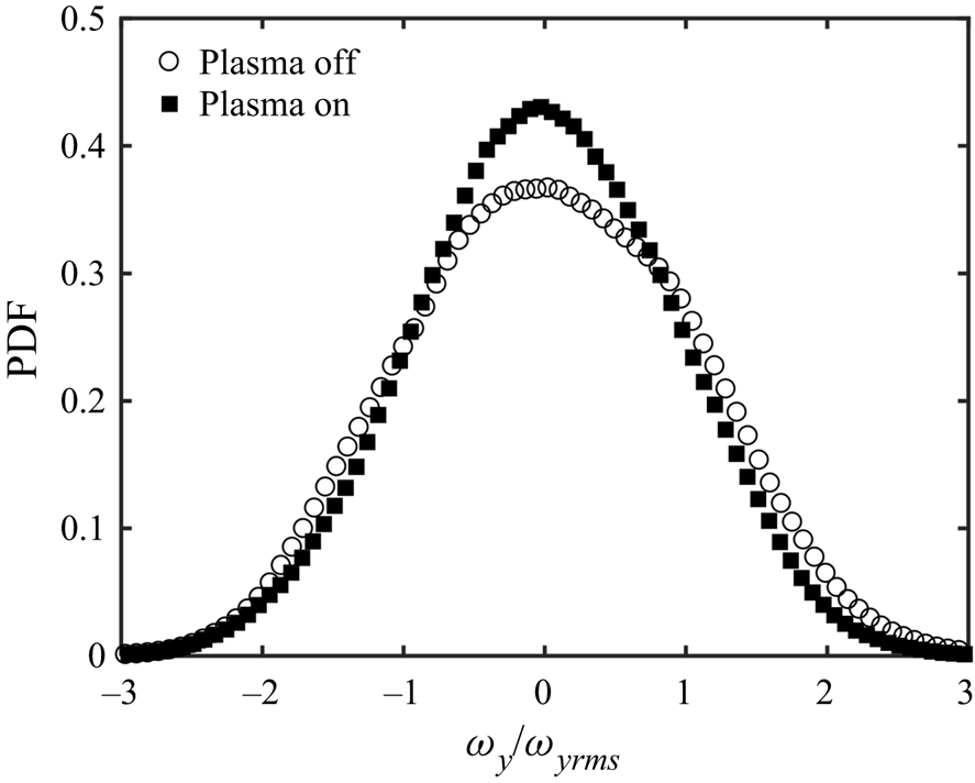
Figure 22. PDF of the normalized wall-normal vorticity ω_y/ω_yrms calculated from the PIV data obtained in the plane of y ⁺ = 24 with and without control (configuration B: E = 4.25 kV_p–p). The calculation area is the same as the area of the FE.

4.4. Weakened bursting events

The bursting events play an important role in the dynamics of the TBL and may be affected by DR. The events are detected from the hot-wire-measured fluctuating velocity signal by the variable-interval time-average (VITA) technique (Blackwelder & Kaplan Reference Blackwelder and Kaplan1976). Two important parameters, namely, the averaging duration T ⁺ and the threshold k, need to be carefully chosen to ensure the events to be correctly detected, where T ⁺ must be of the order of the time scale of the burst and k is such that the VITA value of the fluctuating velocity associated with a detected event is larger than $ku_{rms}^2$. Following Choi et al. (Reference Choi, Jukes and Whalley2011), k and T ⁺ are set at 1 and 10, respectively. Figure 23(a) presents a comparison of the ensemble-averaged u ⁺, i.e. ${\langle {u^ + }\rangle _t}$, between uncontrolled and controlled cases, where ${\langle \,\rangle _t}$ denotes the ensemble averaging based on the VITA detections. In the absence of control, ${\langle {u^ + }\rangle _t}$ agrees reasonably well with Choi et al.'s (Reference Choi, Jukes and Whalley2011) data, which provides a validation for the present VITA analysis. When the plasma control is applied, the strength of the burst, i.e. the difference between the maximum and the minimum ${\langle {u^ + }\rangle _t}$, contracts by 15 % (figure 23a) at z ⁺ = 133 (Region R2) compared to the uncontrolled case, indicating weakened bursting events. Similarly, the bursting event is also found to be impaired at z ⁺ = 0 (R3) – consistent with the suppressed u_rms/U_∞ at y ⁺ = 5 in Regions R2 and R3. On the other hand, there is a small increase (10 %) in the strength of the burst at z ⁺ = 183 (R1), where u_rms/U_∞ increases slightly at y ⁺ = 5 (figure 19e). The weakened burst event is an indication that the streaks are stabilized in the TBL (Bai et al. Reference Bai, Zhou, Zhang, Xu, Wang and Antonia2014), and thus the substantial DR. The slope $\textrm{d}{\langle {u^ + }\rangle _t}/\textrm{d}t$ of the controlled flow at z ⁺ = 0 and 133 is slightly lower than that of the uncontrolled flow (figure 23a). As a rapid increase in ${\langle {u^ + }\rangle _t}$ is directly linked to the sweep motion on the downwash side of the QSVs, the reduced $\textrm{d}{\langle {u^ + }\rangle _t}/\textrm{d}t$ indicates weakened QSVs. A similar observation was also made by Iuso et al. (Reference Iuso, Onorato, Spazzini and Di Cicca2002), who introduced LSSVs in the channel flow using inclined jets. Their VITA analysis suggested a reduced slope ${\langle {\tau _w}\rangle _t}/\textrm{d}t$ of the controlled flow, which was ascribed to the suppressed near-wall longitudinal vortex regeneration by the stabilized streaks. As τ_w is closely correlated with the near-wall streamwise velocity, the reduced $\textrm{d}{\langle {u^ + }\rangle _t}/\textrm{d}t$ is fully consistent with Iuso et al.'s (Reference Iuso, Onorato, Spazzini and Di Cicca2002) VITA analysis. The value of ${\langle {u^ + }\rangle _t}$ further indicates an enhanced ejection at z ⁺ = 183 (R1) compared to the uncontrolled flow, which seems to contradict the downwash of the plasma-induced LSSVs. As the VITA technique involves only the fluctuating velocity, the mean flow should not influence ${\langle {u^ + }\rangle _t}$. Note that the ${\langle {u^ + }\rangle _t}$ signal measured at (x ⁺, y ⁺, z ⁺) = (167, 5, 183) under control and that at (x ⁺, y ⁺, z ⁺) = (167, 15, 183) from the uncontrolled flow are quite similar to each other, as is evident in figure 23(b). As the ejection is closely related to the near-wall QSVs, its enhanced signature at y ⁺ = 5 results apparently from the motion of QSVs towards the wall under the downwash effect of LSSVs.

Figure 23. (a) Ensemble-averaged streamwise fluctuating velocity ${\langle {u^ + }\rangle _t}$ based on VITA detection from hot-wire results. The angle bracket with subscript t, i.e. ${\langle \,\rangle _t}$, denotes the ensemble averaging based on the VITA detections. Ensemble averaging parameter: k = 1, T ⁺ = 10. Measuring location: (x ⁺, y ⁺) = (167, 5). Control parameter: E = 4.25 kV_p–p (configuration B). (b) Comparison of ${\langle {u^ + }\rangle _t}$ between the uncontrolled flow at (x ⁺, y ⁺, z ⁺) = (167, 15, 183) and controlled flow at (x ⁺, y ⁺, z ⁺) = (167, 5, 183).

4.5. Dissipation and production of the TKE budget

The dissipation and production are the dominant terms in the TKE budget near the wall (Pope Reference Pope2001), and their changes may provide insight into the mechanism behind the DR. The dissipation ε is estimated through only one of its 12 components, i.e.$\;\overline {{{(\textrm{d}{u}/\textrm{d}{y})}^2}} $, which accounts for nearly 80 % of the total dissipation in the viscous sublayer and 41 %–72 % in the buffer layer (Antonia, Kim & Browne Reference Antonia, Kim and Browne1991; Qiao, Xu & Zhou Reference Qiao, Xu and Zhou2019). The standard uncertainty ${s_{\overline {{{(\textrm{d}u/\textrm{d}y)}^2}} }}$ of $\overline {{{(\textrm{d}{u}/\textrm{d}{y})}^2}} $, is calculated as

(4.1)\begin{equation}{s_{\overline {{{(\textrm{d}u/\textrm{d}y)}^2}} }} = \sqrt {{{(\overline {{{(\textrm{d}u/\textrm{d}y)}^2}} )}^2} + {{\left( {\sqrt 2 {\sigma_{{\gamma_{\textrm{d}u/\textrm{d}y}}}}\overline {{\gamma_{\textrm{d}u/\textrm{d}y}}} \sqrt {1 + \frac{{\sigma_{{\gamma_{\textrm{d}u/\textrm{d}y}}}^2}}{{2{{\overline {{\gamma_{\textrm{d}u/\textrm{d}y}}} }^2}}}} } \right)}^2}} \sqrt {\frac{2}{{{N_p}}}} ,\end{equation}

where N_p is the number of PIV image pairs, ${\gamma _{\textrm{d}u/\textrm{d}y}}$ is the measurement uncertainty of du/dy, $\overline {{\gamma _{\textrm{d}u/\textrm{d}y}}} $ and ${\sigma _{{\gamma _{\textrm{d}u/\textrm{d}y}}}}$ are the time-averaged value and the standard deviation of ${\gamma _{\textrm{d}u/\textrm{d}y}}$, respectively. The error bars in figure 24(a,b) are plotted as $1.96{s_{\overline {{{(\textrm{d}u/\textrm{d}y)}^2}} }}$, which corresponds to a 95 % confidence interval. In the absence of control, $\overline {{{(\textrm{d}u/\textrm{d}y)}^2}} $ agrees well with Qiao et al.'s (Reference Qiao, Xu and Zhou2019) measurement using a probe of two parallel hot-wires and reasonably well with Antonia et al.'s (Reference Antonia, Kim and Browne1991) DNS data. Under control, the near-wall $\overline {{{(\textrm{d}{u^ + }/\textrm{d}{y^ + })}^2}}$ at z ⁺ = 133 and 0 in Regions R2 and R3, respectively, becomes much larger than that of the uncontrolled case. The greatly increased dissipation is consistent with the substantial DR (Qiao, Wu & Zhou Reference Qiao, Wu and Zhou2018). The $\overline {{{(\textrm{d}{u^ + }/\textrm{d}{y^ + })}^2}} $ becomes smaller at z ⁺ = 183 in Region 1, where drag increases. However, $\overline {{{(\textrm{d}{u^\ast }/\textrm{d}{y^\ast })}^2}} $, normalized by the outer scales, with control deviates only slightly from that without control in all the three regions (figure 24b). Apparently, the variation in $\overline {{{(\textrm{d}{u^ + }/\textrm{d}{y^ + })}^2}} $ (figure 24a) with and without control is largely attributed to the difference in the scaling parameters, namely, local friction velocity and viscous length scale.

Figure 24. Profiles of $\overline {{{(\textrm{d}u/\textrm{d}y)}^2}} $ (a,b) of the mean turbulent energy dissipation and production $ - \overline {uv} (\textrm{d}\bar{U}/\textrm{d}y)$ (c,d) in inner scale (a,c) and outer scale (b,d), respectively. Control parameter: E = 4.25 kV_p–p (configuration B); x ⁺ = 167.

The measured turbulent energy production $ - \overline {{u^ + }{v^ + }} (\textrm{d}\overline {{U^ + }} /\textrm{d}{y^ + })$ in the absence of control (figure 24c) agrees reasonably well with Spalart's (Reference Spalart1988) DNS data, albeit with a small departure. This departure is probably due to the limited spatial resolution of the PIV measurements, as reported in Mizumoto et al. (Reference Mizumoto, Hosokawa, Suzuki and Tomiyama2012). The spatial resolution is 1 wall unit in the near-wall region for Spalart's (Reference Spalart1988) data but 3.75 wall units (0.56 mm) for our PIV data. The standard uncertainty s_P of the production term $ - \overline {uv} (\textrm{d}\bar{U}/\textrm{d}y)$ is calculated through ${s_P} = \sqrt {{{(\overline {uv} )}^2}s_{\textrm{d}\bar{U}/\textrm{d}y}^2 + {{(\textrm{d}\bar{U}/\textrm{d}y)}^2}s_{\overline{uv}}^{2}}$, where ${s_{\textrm{d}\bar{U}/\textrm{d}y}}$ and ${s_{\overline {uv} }}$ are the standard uncertainties of $\textrm{d}\bar{U}/\textrm{d}y$ and $\overline {uv} $, respectively (Sciacchitano & Wieneke Reference Sciacchitano and Wieneke2016). The error bars are plotted in figure 24(c,d) as 1.96 s_P, corresponding to a 95 % confidence interval. The maximum turbulent energy production is 0.25 at y ⁺ ≈ 14 without control. Like $\overline {{{(\textrm{d}{u^ + }/\textrm{d}{y^ + })}^2}} $, $ - \overline {{u^ + }{v^ + }} (\textrm{d}\overline {{U^ + }} /\textrm{d}{y^ + })$ goes up significantly at z ⁺ = 133 in Region R2 and z ⁺ = 0 in Region R3 but drops at z ⁺ = 183 in Region R1 (figure 24c). This is ascribed to the significantly changed local friction velocity and viscous length scale under control. For example, the friction velocity decreases from 0.105 m s⁻¹ in no control to 0.077 m s⁻¹ under control at z ⁺ = 133 in Region R2 and increases to 0.121 m s⁻¹ under control at z ⁺ = 183 in Region R1. However, when normalized by the outer scales (figure 24d), $ - \overline {{u^\ast }{v^\ast }} (\textrm{d}\overline {{U^\ast }} /\textrm{d}{y^\ast })$ is substantially reduced near the wall for the two DR regions, though a slight increase is observed at z ⁺ = 183 in Region R1. Compared with the uncontrolled case, the peak of $ - \overline {{u^\ast }{v^\ast }} (\textrm{d}\overline {{U^\ast }} /\textrm{d}{y^\ast })$ retreats by approximately 26 %, 16 % and 10 % at z ⁺ = 133, 183 and 0, respectively. This retreat is fully consistent with the stabilized streaks (figure 20). The following discussion on production and dissipation will focus on the results normalized by the outer scales (figure 24b,d). Note that the location of peak TKE production changes once the control is applied. For instance, the TKE production peak at z ⁺ = 133 moves away from the wall due to the upwash of the plasma-generated LSSVs but shifts toward the wall at z ⁺ = 183 because of the downwash of the vortices (figure 24d). As the QSVs are responsible for the production of TKE in the TBL (Wallace Reference Wallace2016), this shift in the production peak suggests the movement/alteration of the QSVs by the LSSVs. At z ⁺ = 133 and 0, the QSVs are lifted away from the wall due to the upwash of the plasma-generated vortices, which also accounts for the DR (Tardu Reference Tardu2001). However, the energy production at 0.028 < y/δ < 0.301 (16 < y ⁺ < 170) is increased compared to the uncontrolled case due to the lifted QSVs, which is also consistent with the increased u_rms/U_∞ in this region (figure 19d). At z ⁺ = 183, the downwash of the LSSVs pushes the QSVs towards the wall. Thus, the production is mostly confined to the near-wall region, accounting for an increased production for y/δ < 0.012 (y ⁺ < 7) but a reduced production further away for y/δ = 0.012–0.109 (y ⁺ = 7–60). A similar observation was also made from the DNS results of Mahfoze & Laizet (Reference Mahfoze and Laizet2017), who superimposed plasma-induced spanwise flow oscillation near the wall in a turbulent channel flow of relatively low Re_τ ( = 180). They achieved a DR of 24 % under the optimal control parameters. Accordingly, the TKE production peak was reduced by 19 %, with its location shifted away from the wall.

4.6. DR mechanism

A DR mechanism is proposed based on the distribution of the local DR and the various aspects of the flow captured with and without control. The key strategy of the present plasma control is to manipulate the near-wall coherent structures, which are accountable for the high skin friction in the TBL. It has been well established that the near-wall turbulence regeneration cycle plays a crucial role in the sustenance of the coherent structures (e.g. Kim Reference Kim2011). As such, interrupting this cycle may lead to substantially weakened near-wall coherent structures, resulting in a reduction in the skin friction. Several DR techniques for the TBL have been developed based on this concept, including spanwise wall oscillation (e.g. Choi et al. Reference Choi, Debisschop and Clayton1998; Agostini, Touber & Leschziner Reference Agostini, Touber and Leschziner2014) or a spanwise/transverse or streamwise-travelling wave (e.g. Du et al. Reference Du, Symeonidis and Karniadakis2002; Quadrio et al. Reference Quadrio, Ricco and Viotti2009; Bai et al. Reference Bai, Zhou, Zhang, Xu, Wang and Antonia2014; Qiao et al. Reference Qiao, Zhou and Wu2017).

In present study, the plasma actuators generate counter-rotating LSSVs (figure 15). These ‘externally’ introduced vortices and their associated spanwise wall jets act to merge the streaks. As a result, the streaks are broader and have reduced meandering (figure 20), which is also reflected by the reduced wall-normal vorticity ω_y (figure 22) – both explained by Schoppa & Hussain (Reference Schoppa and Hussain2002). The streaks are pushed into the central region of each actuator pair by the plasma-generated spanwise flow, and moved away from the wall by the upwash motion of these external vortices (figure 20). All the observations along with the comparison in the bursts between the controlled and uncontrolled flows (figure 23) point to the substantially stabilized streaks (Yao et al. Reference Yao, Chen and Hussain2018).

The instability of streaks, especially that due to the transient growth, is the essential element for the generation of QSVs (Schoppa & Hussain Reference Schoppa and Hussain2002; Kim Reference Kim2011) in the turbulence regeneration cycle. Naturally, the stabilized streaky structures will interrupt this cycle and subsequently suppress the generation of new QSVs, leading to weakened near-wall coherent structures, which is confirmed from the reduced turbulence intensity and TKE production in Regions R2 and R3 (figures 19 and 24d). The weakened QSVs and merged streaks under the control of externally generated LSSVs are also observed in Yao et al.'s (Reference Yao, Chen and Hussain2018) DNS and Iuso et al.'s (Reference Iuso, Onorato, Spazzini and Di Cicca2002) experiments. As a result, the skin friction is substantially reduced (figure 14). Interestingly, these LSSVs change little the turbulent energy dissipation (figure 24b), unlike some other techniques such as the piezo-ceramic-actuator-generated spanwise-travelling wave (Bai et al. Reference Bai, Zhou, Zhang, Xu, Wang and Antonia2014; Qiao et al. Reference Qiao, Zhou and Wu2017) where the enhancement of the dissipation in the near-wall region is one of the keys for DR.