


1. Introduction
It was recently discovered that when long-crested irregular waves propagate from deeper to shallower water, there can be a local maximum of skewness and kurtosis of the surface elevation just inside the shallower part (Trulsen et al. Reference Trulsen, Zeng and Gramstad2012). For the velocity field, only the skewness appears to display a similar local maximum in the shallower part, while the kurtosis does not (Trulsen et al. Reference Trulsen, Raustøl, Jorde and Rye2020). It was also discovered that behind a shoal, there can be a local negative minimum of skewness for both surface elevation and velocity fields, while only the velocity field shows an anomaly for the kurtosis, with a local maximum (Trulsen et al. Reference Trulsen, Raustøl, Jorde and Rye2020).
A large body of experimental and numerical work has reproduced the spatial anomalies of skewness and kurtosis of the surface elevation over depth transitions. The behaviour has been captured by Korteweg–de Vries models (Sergeeva et al. Reference Sergeeva, Pelinovsky and Talipova2011; Bolles et al. Reference Bolles, Speer and Moore2019; Majda et al. Reference Majda, Moore and Qi2019; Majda & Qi Reference Majda and Qi2020; Moore et al. Reference Moore, Bolles, Majda and Qi2020), Boussinesq models (Gramstad et al. Reference Gramstad, Zeng, Trulsen and Pedersen2013) and other higher-order potential models (e.g.Viotti & Dias Reference Viotti and Dias2014; Lawrence et al. Reference Lawrence, Trulsen and Gramstad2021; Zhang & Benoit Reference Zhang and Benoit2021).
Extending this to short-crested waves propagating over a two-dimensional shoal, it was reported by Ducrozet & Gouin (Reference Ducrozet and Gouin2017) that the enhancement of extreme waves is reduced compared to incoming long-crested waves. On the other hand, Lawrence et al. (Reference Lawrence, Trulsen and Gramstad2022) found an increase in the extreme statistics for unidirectional waves propagating over a circular or semicircular three-dimensional shoal, provoking short-crested waves after the shoal. These observations should be taken into account when interpreting field observations such as those of Bitner (Reference Bitner1980), Cherneva et al. (Reference Cherneva, Petrova, Andreeva and Guedes Soares2005) and Teutsch et al. (Reference Teutsch, Weisser, Moeller and Krueger2020).
Explanations for the occurrence of freak surface waves have been suggested by Li et al. (Reference Li, Draycott, Adcock and van den Bremer2021a ,Reference Li, Draycott, Zheng, Lin, Adcock and van den Bremer b ,Reference Li, Zheng, Lin, Adcock and van den Bremer c ), who discuss the generation of new free wavepackets. Zhang et al. (Reference Zhang, Benoit, Kimmoun, Chabchoub and Hsu2019) and Zheng et al. (Reference Zheng, Lin, Li, Adcock, Li and van den Bremer2020), however, point to the transition into a new equilibrium state when the waves propagate over a step.
The extreme statistics of the velocity field under irregular waves over a shoal, earlier observed experimentally by Trulsen et al. (Reference Trulsen, Raustøl, Jorde and Rye2020), were later reproduced numerically by Lawrence et al. (Reference Lawrence, Trulsen and Gramstad2021), Zhang & Benoit (Reference Zhang and Benoit2021) and Zhang et al. (Reference Zhang, Ma and Benoit2024). In addition to the investigation of the velocity, numerical simulation of the acceleration has been done by Zhang & Benoit (Reference Zhang and Benoit2021), Benoit et al. (Reference Benoit, Zhang and Ma2024)and Zhang et al. (Reference Zhang, Ma and Benoit2024), suggesting that the horizontal acceleration distribution is changing differently from the surface elevation and the horizontal velocity. We speculate whether the anomalies in velocity and acceleration statistics can have consequences for the statistical distribution of forces experienced by structures submerged on the lee side of a shoal.
On deep water, the wave forces experienced by submerged cylinders have been studied for several decades. For regular waves, Dean (Reference Dean1948) studied the reflection from the cylinder, and how the surface waves were modified when passing over the cylinder. His calculations were succeeded by several articles following the same line of discussion, calculating the forces on the cylinder as well (Ursell Reference Ursell1950a,b ; Ogilvie Reference Ogilvie1963; Davis & Hood Reference Davis and Hood1976; Mehlum Reference Mehlum1980; Grue & Palm Reference Grue and Palm1984; Chaplin Reference Chaplin1984; Vada Reference Vada1987; Arena Reference Arena1999). Extending this to irregular waves, Boccotti (Reference Boccotti1996), Arena (Reference Arena2002, Reference Arena2006) and Romolo et al. (Reference Romolo, Malara, Barbaro and Arena2009) studied the spectrum and the probability density function of the forces, and compared the forces to the Froude–Krylov force.
In the presence of a sloping bottom, the wave force on a horizontal cylinder located over a shoaling area was investigated by Sundar et al. (Reference Sundar, Roopsekhar, Schlurmann and Abbasi2004). They observed a Gaussian probability distribution for the vertical and horizontal forces. Recently, Li et al. (Reference Li, Tang, Li, Draycott, van den Bremer and Adcock2023) computed the statistics of drag forces on a vertical cylinder over an abrupt depth transition. They followed the approach suggested by Klahn et al. (Reference Klahn, Madsen and Fuhrman2021), using the drag term from the Morison equation (Morison et al. Reference Morison, Johnson and Schaaf1950) with the velocity computed by a numerical model of Engsig-Karup et al. (Reference Engsig-Karup, Bingham and Lindberg2009). This did not take into account any interaction with the cylinder. From this, Li et al. (Reference Li, Tang, Li, Draycott, van den Bremer and Adcock2023) reported an increase in extreme force statistics at the top of the up-slope, as could be anticipated from the extreme surface elevation statistics. There appears to be a lack of investigation of wave forces experienced over the down-slope and behind a shoal, at the location where the above-mentioned anomaly of kurtosis in the velocity field is experienced.
The goal of this paper is to study the statistics of extreme wave forces for a horizontal submerged cylinder over the down-slope of a shoal, at the location of an anomaly in the kurtosis of the velocity field. The wave regime applied is similar to the most dramatic runs of Trulsen et al. (Reference Trulsen, Raustøl, Jorde and Rye2020). We compare the force statistics with the corresponding statistics of the horizontal velocity field, horizontal acceleration and the surface elevation. We find that the extreme statistics of surface elevation, fluid velocity, fluid acceleration and resulting forces are all different from each other. Extreme statistics is here understood as high values of skewness and kurtosis.
2. Experiment
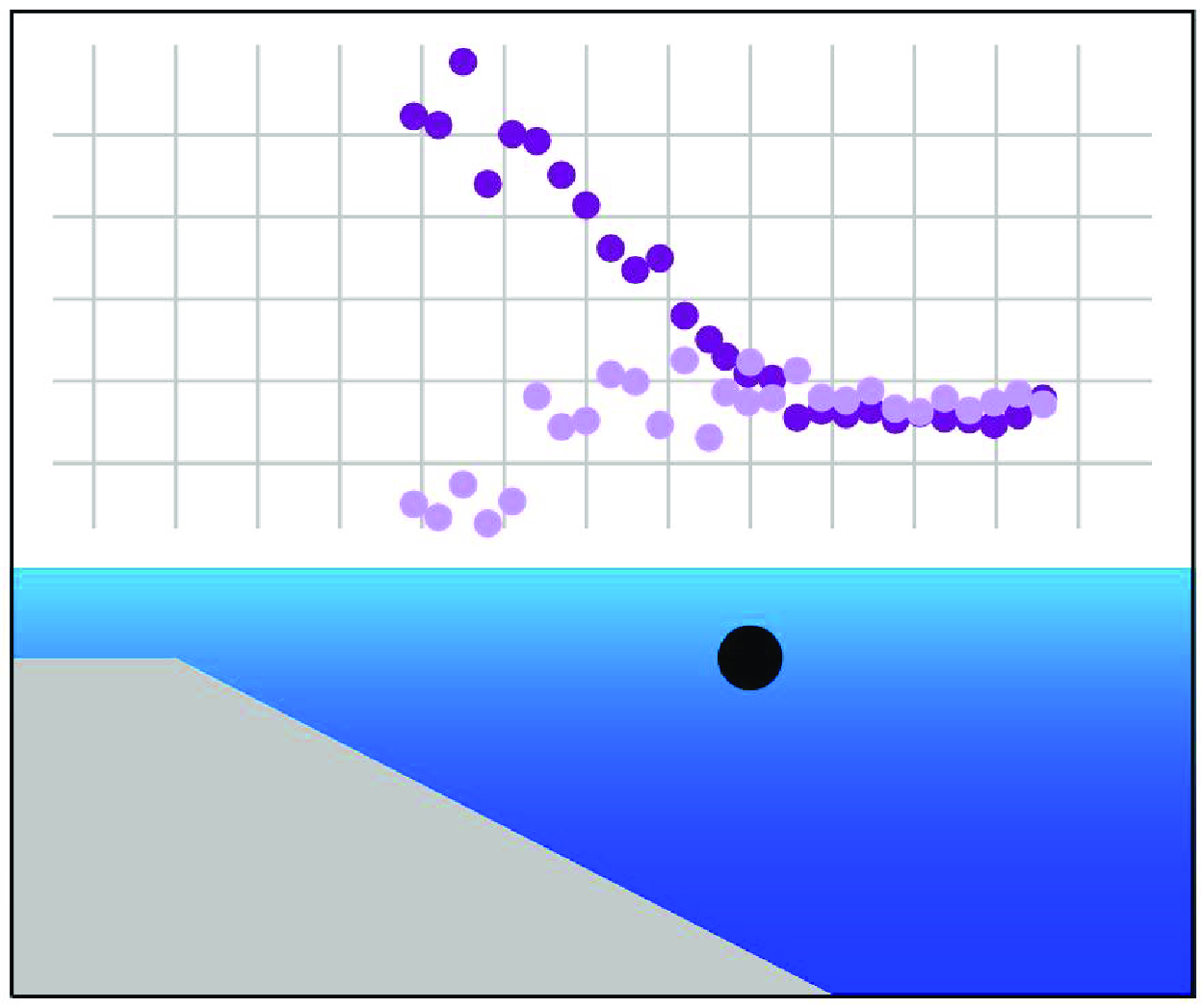
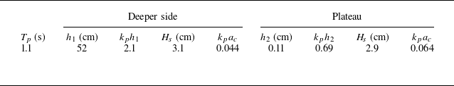
The experimental set-up is similar to that employed in Trulsen et al. (Reference Trulsen, Raustøl, Jorde and Rye2020), with the important difference that the shoal is now asymmetric, with a longer up-slope and a shorter down-slope, as shown in figure 1. The shoal is placed in a flume of length approximately
 $25\,\rm m$
and width
$25\,\rm m$
and width
 $0.5\,\rm m$
. The horizontal
$0.5\,\rm m$
. The horizontal
 $x$
-axis has its origin
$x$
-axis has its origin
 $x=0\,\rm m$
at the beginning of the plateau, which is
$x=0\,\rm m$
at the beginning of the plateau, which is
 $10.16\,\rm m$
from the wave paddle. Waves are damped at the end of the flume, with a 1 m beach of expanded metal ending at
$10.16\,\rm m$
from the wave paddle. Waves are damped at the end of the flume, with a 1 m beach of expanded metal ending at
 $x=12.46\,\rm m$
, with approximately
$x=12.46\,\rm m$
, with approximately
 $20^\circ$
slope. Behind the beach, further damping by expanded metal is applied, all this resulting in approximately
$20^\circ$
slope. Behind the beach, further damping by expanded metal is applied, all this resulting in approximately
 $4\,\%$
reflection of the waves (Støle-Hentschel et al. Reference Støle-Hentschel, Trulsen, Rye and Raustøl2018). The depth in the deeper parts is
$4\,\%$
reflection of the waves (Støle-Hentschel et al. Reference Støle-Hentschel, Trulsen, Rye and Raustøl2018). The depth in the deeper parts is
 $h_1=52\,\rm cm$
, while over the plateau, the depth is
$h_1=52\,\rm cm$
, while over the plateau, the depth is
 $h_2=11\,\rm cm$
. Reference measurements are also done without the shoal in the flume.
$h_2=11\,\rm cm$
. Reference measurements are also done without the shoal in the flume.
Four ultrasound probes measure the surface elevation along the centreline of the wave flume. One is always at
 $x=-2.9\,\rm m$
, while the others are moved. The distance between the second and third is
$x=-2.9\,\rm m$
, while the others are moved. The distance between the second and third is
 $75.5\,\rm cm$
, and the distance between the third and fourth is
$75.5\,\rm cm$
, and the distance between the third and fourth is
 $70.0\,\rm cm$
. The sample rate is set to 125 Hz, and the probes are 120 mm above the water level at equilibrium. In § 4, only results from the down-slope area will be reported.
$70.0\,\rm cm$
. The sample rate is set to 125 Hz, and the probes are 120 mm above the water level at equilibrium. In § 4, only results from the down-slope area will be reported.

Figure 1. Set-up of the measurement campaign. (a) Typical configuration of a single experimental run with water (blue), shoal (grey), four surface probes (hollow black circles) and submerged cylinder (filled black circle shown in actual size). (b) Indication of all measurement locations for surface probes during the ADV measurements (hollow red circles), surface probes during the force measurements (hollow black circles), ADV (red dots) and submerged cylinder (black dots, smaller than actual size of the cylinder). The wavemaker farther out to the left, and the damping beach farther out to the right, are not shown.
Within the water, measurements are made of either the velocity field in the absence of a cylinder, or forces on the cylinder.
For the velocity measurements, an acoustic Doppler velocimeter (ADV) is placed
 $5.5\,\rm cm$
below the surface at equilibrium, over the down-slope. The ADV is positioned horizontally and pointing towards the wave paddle, to get the most accurate measurements in the horizontal direction, and to avoid disturbing the wave-induced flow field. The mean is taken of the data from the two transducers that are pointing in the same horizontal direction on the ADV. The sample rate is set to 200 Hz, the nominal velocity range is
$5.5\,\rm cm$
below the surface at equilibrium, over the down-slope. The ADV is positioned horizontally and pointing towards the wave paddle, to get the most accurate measurements in the horizontal direction, and to avoid disturbing the wave-induced flow field. The mean is taken of the data from the two transducers that are pointing in the same horizontal direction on the ADV. The sample rate is set to 200 Hz, the nominal velocity range is
 $0.3\,\text{m}\,\text{s}^{-1}$
, the transmit length is 1.8 mm, and the sampling volume has length 7.0 mm. We use polyamid seeding particles with diameter 50
$0.3\,\text{m}\,\text{s}^{-1}$
, the transmit length is 1.8 mm, and the sampling volume has length 7.0 mm. We use polyamid seeding particles with diameter 50
 $\mu\rm m$
.
$\mu\rm m$
.
For the force measurements, a horizontal submerged cylinder parallel to the wave crests is installed over the down-slope, with centre
 $h_{cyl}=10.7\,\rm cm$
from the water surface at equilibrium. This distance is such that the cylinder will not get dry when the waves are propagating over it, and such that the waves do not break over it. The diameter of the cylinder is
$h_{cyl}=10.7\,\rm cm$
from the water surface at equilibrium. This distance is such that the cylinder will not get dry when the waves are propagating over it, and such that the waves do not break over it. The diameter of the cylinder is
 $d=7.5\,\rm cm$
. The force measurements are made only over the down-slope of the shoal. See figure 1 for a visual representation of the set-up. Two force transducers, each of length
$d=7.5\,\rm cm$
. The force measurements are made only over the down-slope of the shoal. See figure 1 for a visual representation of the set-up. Two force transducers, each of length
 $12.5\,\rm cm$
, are placed in the cylinder, and fastened on the flume walls. They are based on the Wheatstone Bridge, and measure both vertical and horizontal forces. The data from the two transducers are added to get the total force on the cylinder in each direction. The sample rate is set to 200 Hz. The product
$12.5\,\rm cm$
, are placed in the cylinder, and fastened on the flume walls. They are based on the Wheatstone Bridge, and measure both vertical and horizontal forces. The data from the two transducers are added to get the total force on the cylinder in each direction. The sample rate is set to 200 Hz. The product
 $k_pd$
between the peak wavenumber of the surface elevation
$k_pd$
between the peak wavenumber of the surface elevation
 $k_p$
and the diameter of the cylinder
$k_p$
and the diameter of the cylinder
 $d$
ranges between
$d$
ranges between
 $0.30$
and
$0.30$
and
 $0.35$
for the positions where forces were measured over the down-slope of the shoal. The product
$0.35$
for the positions where forces were measured over the down-slope of the shoal. The product
 $k_ph_{cyl}$
is between 0.50 and 0.43. The ratio
$k_ph_{cyl}$
is between 0.50 and 0.43. The ratio
 $e/d$
between the distance from cylinder bottom to the seabed
$e/d$
between the distance from cylinder bottom to the seabed
 $e$
, and the diameter of the cylinder
$e$
, and the diameter of the cylinder
 $d$
, ranges between 1.52 and 5.0. We measure experimentally that the natural frequency of the cylinder placed
$d$
, ranges between 1.52 and 5.0. We measure experimentally that the natural frequency of the cylinder placed
 $10.7\,\rm cm$
under the still surface in water of depth
$10.7\,\rm cm$
under the still surface in water of depth
 $52\,\rm cm$
is approximately
$52\,\rm cm$
is approximately
 $115\,\rm Hz$
in both horizontal and vertical directions. This means that the natural frequency is well above the frequency range in which we are interested.
$115\,\rm Hz$
in both horizontal and vertical directions. This means that the natural frequency is well above the frequency range in which we are interested.
The trigger for the measurements is synchronized between the ultrasound probes and the ADV or force transducers. One of the ultrasound probes is always directly above the measurement volume for the ADV or the centre of the cylinder. Hence this probe always measures the same wave phase as the ADV or the force transducers.
The long-crested irregular waves are generated according to the Pierson–Moskowitz spectrum (Pierson & Moskowitz Reference Pierson and Moskowitz1964), which is a special case of the JONSWAP spectrum, with the
 $\gamma$
-parameter set to 1 (Hasselmann et al. Reference Hasselmann, Barnett, Bouws, Carlson, Cartwright, Enke, Ewing, Gienapp, Hasselmann and Kruseman1973). This choice of spectrum is different from that of Trulsen et al. (Reference Trulsen, Raustøl, Jorde and Rye2020) and several others who used the JONSWAP spectrum with
$\gamma$
-parameter set to 1 (Hasselmann et al. Reference Hasselmann, Barnett, Bouws, Carlson, Cartwright, Enke, Ewing, Gienapp, Hasselmann and Kruseman1973). This choice of spectrum is different from that of Trulsen et al. (Reference Trulsen, Raustøl, Jorde and Rye2020) and several others who used the JONSWAP spectrum with
 $\gamma =3.3$
. The nominal peak period is
$\gamma =3.3$
. The nominal peak period is
 $T_p=1.1\,\rm s$
. The amplitude factor is set to achieve the steepest waves possible without causing them to break or spill. The frequency range is
$T_p=1.1\,\rm s$
. The amplitude factor is set to achieve the steepest waves possible without causing them to break or spill. The frequency range is
 $3.66\text { rad}\,{\rm s^-{^1}}\leqslant \omega \leqslant 16.56\text { rad}\,{\rm s^-{^1}}$
. For each run, measurements are done for 20 minutes, beginning after the wave front of the wave train has propagated past the probes, and ending before the tail reaches them. More details can be found in table 1. Here, the dimensionless depth
$3.66\text { rad}\,{\rm s^-{^1}}\leqslant \omega \leqslant 16.56\text { rad}\,{\rm s^-{^1}}$
. For each run, measurements are done for 20 minutes, beginning after the wave front of the wave train has propagated past the probes, and ending before the tail reaches them. More details can be found in table 1. Here, the dimensionless depth
 $k_ph$
, significant wave height
$k_ph$
, significant wave height
 $H_s$
and steepness
$H_s$
and steepness
 $k_pa_c$
are averages over all surface measurements done in front of the shoal or on the plateau of the shoal. The peak wavenumber is derived from the linear dispersion relation
$k_pa_c$
are averages over all surface measurements done in front of the shoal or on the plateau of the shoal. The peak wavenumber is derived from the linear dispersion relation
 $\omega _p^2 = g k_p \tanh (k_p h)$
at each location, where
$\omega _p^2 = g k_p \tanh (k_p h)$
at each location, where
 $\omega _p$
is the peak of the power spectrum of the surface elevation,
$\omega _p$
is the peak of the power spectrum of the surface elevation,
 $g$
is the acceleration of gravity, and
$g$
is the acceleration of gravity, and
 $h$
is the depth at each particular location. The characteristic amplitude of the surface elevation is
$h$
is the depth at each particular location. The characteristic amplitude of the surface elevation is
 $a_c = \sqrt {2}\sigma$
, and the significant wave height is
$a_c = \sqrt {2}\sigma$
, and the significant wave height is
 $H_s=4\sigma$
, where
$H_s=4\sigma$
, where
 $\sigma$
is the standard deviation of the surface elevation.
$\sigma$
is the standard deviation of the surface elevation.
Table 1. Key parameters for the surface elevation in the experiments. Nominal peak period
 $T_p$
is from the input time series. Dimensionless depth
$T_p$
is from the input time series. Dimensionless depth
 $k_ph$
, significant wave height
$k_ph$
, significant wave height
 $H_s$
and steepness
$H_s$
and steepness
 $k_pa_c$
are averages over all surface measurements done in front of the shoal or on the plateau of the shoal.
$k_pa_c$
are averages over all surface measurements done in front of the shoal or on the plateau of the shoal.
3. Analysis
3.1. Wave regime
We anticipate that a useful characterization of the transition between wave regimes is indicated by the diagram of Le Méhauté (Reference Le Méhauté1976), as suggested by Zhang & Benoit (Reference Zhang and Benoit2021). Previously, the diagram used for this purpose in Trulsen et al. (Reference Trulsen, Raustøl, Jorde and Rye2020) took into account only the water depth and not the wave amplitude. While the diagram of Le Méhauté was originally intended for monochromatic waves of height
 $H$
and period
$H$
and period
 $T$
, we here employ the significant wave height
$T$
, we here employ the significant wave height
 $H_s$
and nominal peak period
$H_s$
and nominal peak period
 $T_p$
of the irregular wave fields in front of the shoal and on top of the plateau; see figure 2. No breaking or spilling waves were seen in these experiments, in agreement with the diagram. We anticipate that the occurrence of large skewness and kurtosis on top of the shoal may depend on the transition between the different regimes suggested in figure 2.
$T_p$
of the irregular wave fields in front of the shoal and on top of the plateau; see figure 2. No breaking or spilling waves were seen in these experiments, in agreement with the diagram. We anticipate that the occurrence of large skewness and kurtosis on top of the shoal may depend on the transition between the different regimes suggested in figure 2.

Figure 2. Partial Le Méhauté (Reference Le Méhauté1976) diagram for runs 1, 2, 3, 6 and 8 in Trulsen et al. (Reference Trulsen, Raustøl, Jorde and Rye2020) (TRJR) and for the measurements in our experiment (ST). Each pair of symbols indicates the change in wave conditions from the deeper side (points to the right) to the shallower side (points to the left). Here,
 $h$
is the depth. For
$h$
is the depth. For
 $H$
, we substitute the significant wave height. For
$H$
, we substitute the significant wave height. For
 $T$
and
$T$
and
 $L$
, we substitute the nominal peak period and the corresponding wavelength. The condition on the Ursell number
$L$
, we substitute the nominal peak period and the corresponding wavelength. The condition on the Ursell number
 $U_r = L^2 H/h^3 = 26$
suggests the parametric boundary between small-amplitude wave theory and long wave theory. The condition
$U_r = L^2 H/h^3 = 26$
suggests the parametric boundary between small-amplitude wave theory and long wave theory. The condition
 $H/h = 0.78$
suggests the breaking limit of solitary waves. The two vertical lines suggest parametric boundaries between shallow, intermediate and deep water.
$H/h = 0.78$
suggests the breaking limit of solitary waves. The two vertical lines suggest parametric boundaries between shallow, intermediate and deep water.
3.2. Force regime
Regarding our interest in whether the extreme statistics for the horizontal force changes in the same way as for the horizontal velocity, it is interesting to estimate what kind of force dominates. The ratio between the drag term and the inertia term in the Morison equation is estimated to be approximately 0.02, which indicates an inertia-dominated regime. The Keulegan–Carpenter (KC) number is calculated by the characteristic amplitude and nominal peak period of the measured horizontal velocity to be between 0.60 and 0.86, depending on the position of the measurement. Since the centre of the cylinder is some centimetres below the ADV measurement volume, we expect an even lower KC number at the position of the cylinder. By this low KC number, according to Chaplin (Reference Chaplin1984), we anticipate that the cylinder will not produce any significant amount of separation in the wake. Our KC number also suggests that inertia dominates the forces (Chaplin Reference Chaplin1984).
To get another view of whether the horizontal force is dominated by drag or inertia, we compute the horizontal local acceleration
 $ax=\partial u/\partial t$
for the inertia term, and
$ax=\partial u/\partial t$
for the inertia term, and
 $u\,|u|$
for the drag term, both computed from the measured horizontal velocity
$u\,|u|$
for the drag term, both computed from the measured horizontal velocity
 $u$
. Their probability density functions (PDFs) are shown in § 4, and indeed support that the horizontal force is dominated by inertia. Thus we calculate the skewness and kurtosis only for the local acceleration and not for
$u$
. Their probability density functions (PDFs) are shown in § 4, and indeed support that the horizontal force is dominated by inertia. Thus we calculate the skewness and kurtosis only for the local acceleration and not for
 $u\,|u|$
. We are aware that our velocity measurements are not positioned at the exact same depth as the centre of the cylinder; however, we are only interested in the qualitative changes of the statistics.
$u\,|u|$
. We are aware that our velocity measurements are not positioned at the exact same depth as the centre of the cylinder; however, we are only interested in the qualitative changes of the statistics.
The local acceleration is computed with a 5-node centred finite difference scheme in the middle points
 \begin{equation} ax_{i}=\frac {1}{12\,\Delta t}\left ( -u_{i+2} + 8u_{i+1} - 8u_{i-1} + u_{i-2} \right ), \end{equation}
and a 5-node forwards finite difference scheme for the first two points,
 \begin{align} ax_{1}=\frac {1}{12\,\Delta t}\left ( -25u_1 + 48u_2 - 36u_3 + 16u_4 - 3u_5 \right ), \end{align}
 \begin{align} ax_{2}=\frac {1}{12\,\Delta t}\left ( -3u_1 - 10u_2 + 18u_3 - 6u_4 + u_5 \right ), \end{align}
and similarly backwards for the last two points. Here,
 $ax=\partial u/\partial t$
is the horizontal acceleration at
$ax=\partial u/\partial t$
is the horizontal acceleration at
 $z=-5.5\,\rm cm$
,
$z=-5.5\,\rm cm$
,
 $u$
is the horizontal velocity measured in the experiments at
$u$
is the horizontal velocity measured in the experiments at
 $z=-5.5\,\rm cm$
,
$z=-5.5\,\rm cm$
,
 $\Delta t$
is the time step, and
$\Delta t$
is the time step, and
 $i=1,2,\ldots ,N$
is the sample number.
$i=1,2,\ldots ,N$
is the sample number.
To get rid of noise, the lowpass function included in Matlab is used, with limit frequency
 $\text{fpass}=3\,\rm Hz$
and lowpass filter steepness set to 0.99.
$\text{fpass}=3\,\rm Hz$
and lowpass filter steepness set to 0.99.
We remark that we have employed the form of Morison equation presented in Morison et al. (Reference Morison, Johnson and Schaaf1950). We are aware that there are several formulations for calculating the total force that are more precise than this, e.g. Rainey (Reference Rainey1989, Reference Rainey1995), but we limit ourselves to the Morison equation, as this is the most widely used formula.
4. Results
We carry out statistical analysis of the results from the measurements, and from
 $u\,|u|$
and acceleration calculations. This is done in order to discuss skewness and kurtosis, as well as probability distribution and exceedance probability.
$u\,|u|$
and acceleration calculations. This is done in order to discuss skewness and kurtosis, as well as probability distribution and exceedance probability.
4.1. Skewness and kurtosis
We study the skewness and kurtosis of the surface elevation, horizontal velocity, horizontal local acceleration, and horizontal and vertical forces. The results are shown in figures 3, 4, 5 and 6. Here, the vertical dashed lines mark the beginning and end of the down-slope behind the shoal. The blue circle marks the skewness or kurtosis measured on a specific location, from similar measurements done without the shoal in the flume. Without the shoal, we assume that the skewness and kurtosis are essentially constant over the region where we do measurements, as indicated by the blue horizontal dashed line.
As shown in figure 3, the skewness of the surface elevation decreases down the slope and has a minimum over the down-slope of the shoal. The kurtosis decreases as well, to a minimum in the middle of the down-slope.

Figure 3. Skewness and kurtosis of surface elevation over the down-slope of the shoal (black). Blue is for measurements without the shoal. Dashed vertical lines mark the beginning and end of the down-slope.

Figure 4. Same as in figure 3, but for horizontal velocity over the down-slope (orange).

Figure 5. Same as in figure 3, but for horizontal acceleration over the down-slope (orange).

Figure 6. Same as in figure 3, but for force in horizontal (circles) and vertical (triangles) directions. Blue is for measurements without the shoal; violet and yellow are for measurements with the shoal.

Figure 7. The PDF of the horizontal force normalized by its standard deviation. With shoal indicated by purple; reference measurement without shoal indicated by dashed blue; Gaussian distribution indicated by green.

Figure 8. Same as in figure 7, but for vertical force (yellow).

Figure 9. Same as in figure 7, but for horizontal velocity (orange).
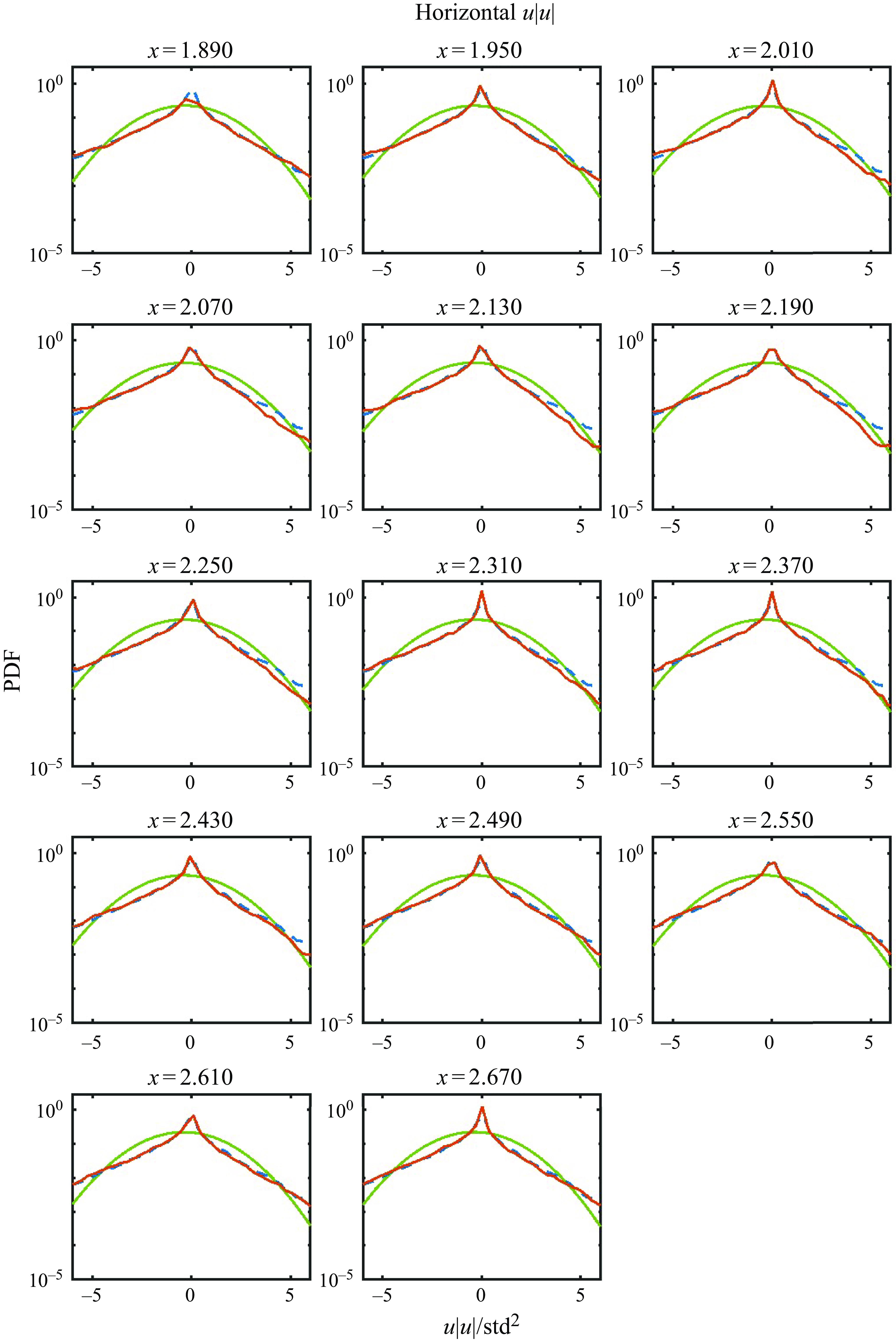
Figure 10. Same as in figure 7, but for
 $u\,|u|$
(orange), where
$u\,|u|$
(orange), where
 $u$
is the horizontal velocity.
$u$
is the horizontal velocity.

Figure 11. Same as in figure 7, but for horizontal acceleration (orange).
The results for ADV measurements are shown in figure 4, giving an indication of the change in statistics for the horizontal velocity over the down-slope of the shoal, at approximately the same positions where forces on the cylinder are measured. The minimum of skewness is at the same position as for surface elevation, while the maximum in kurtosis is at approximately the same location as where the kurtosis for the surface elevation reaches its local minimum.
The skewness and kurtosis of the surface elevation and the velocity field have the same trends as found in earlier work (Gramstad et al. Reference Gramstad, Zeng, Trulsen and Pedersen2013; Lawrence et al. Reference Lawrence, Trulsen and Gramstad2021; Ma et al. Reference Ma, Dong and Ma2014; Trulsen et al. Reference Trulsen, Zeng and Gramstad2012,Reference Trulsen, Raustøl, Jorde and Rye2020), although we have generated waves from the Pierson–Moskowitz spectrum while earlier work was usually based on the JONSWAP spectrum with a larger value of the peakedness parameter.
The results for the horizontal local acceleration shown in figure 5 give trends similar to those that Zhang et al. (Reference Zhang, Ma and Benoit2024) found by calculation of acceleration from the data of Trulsen et al. (Reference Trulsen, Raustøl, Jorde and Rye2020). Compared to measurements over theflat bottom, there is a change in skewness and kurtosis, and the values are closer to the values over the flat bottom for the positions farthest down the slope. The skewness is increasing to a maximum near the end of the down-slope, while the kurtosis is decreasing to a minimum at approximately the same place.
Figure 6 shows the skewness and kurtosis for the horizontal and vertical forces on the down-slope of the shoal. Figure 6(a) shows that the skewness for the horizontal force is decreasing as we go down the slope, and there seems to be a minimum at approximately the end of the slope. For the vertical force, the skewness changes in a different way than for the horizontal force, with always positive skewness as the depth increases. The skewness for the vertical force at position
 $x=1.89\,\rm m$
is the same as for the measurements without a shoal, and it grows and then sinks again when the depth becomes larger. The change in skewness between the positions with shallower water depth and deeper water depth is larger for the horizontal force than for the vertical force.
$x=1.89\,\rm m$
is the same as for the measurements without a shoal, and it grows and then sinks again when the depth becomes larger. The change in skewness between the positions with shallower water depth and deeper water depth is larger for the horizontal force than for the vertical force.
The kurtosis too behaves differently for the vertical force compared to the horizontal force. The kurtosis for the horizontal force increases as the depth becomes larger, then stabilizes at a higher value when we go down the slope, compared to close to the plateau. The kurtosis of the vertical force, on the other hand, increases somewhat, then decreases again towards the kurtosis of the measurements without a shoal.
Comparing figures 3, 4, 5 and 6, we see that the horizontal force does not follow the same trend as the surface elevation, the horizontal velocity or the horizontal acceleration. The skewness of the horizontal force decreases similarly to the surface elevation and horizontal velocity, but with a minimum later on the down-slope. The kurtosis of the horizontal force first increases, then maintains a constant value behind the shoal, quite different from the surface elevation, velocity and acceleration.
4.2. The PDF
In figures 7, 8, 9, 10 and 11, we present probability distributions of the forces, the horizontal velocity, the horizontal local acceleration and horizontal
 $u\,|u|$
for selected positions, normalized by the standard deviation of the measurements at the same position. Measurements without a shoal are shown for reference. The Gaussian distribution at each position is also shown, for comparison.
$u\,|u|$
for selected positions, normalized by the standard deviation of the measurements at the same position. Measurements without a shoal are shown for reference. The Gaussian distribution at each position is also shown, for comparison.
The horizontal force distribution is shown in figure 7. At several positions, the PDF is more positively skewed for the measurements done with a shoal than without a shoal. Hence there is a higher probability for large positive forces over the shoal than over the flat bottom. Compared to the Gaussian distribution, the force distribution is more positively skewed at the first positions, which is in agreement with the skewness shown in figure 6 at these positions. This shows that there is a higher probability for large forces in the same direction as the waves propagate, compared to the indication from the Gaussian distribution. As the water depth increases, the PDF becomes wider, allowing a higher probability for large forces in both positive and negative horizontal directions, compared to in shallower water. Nevertheless, for the largest forces, the PDF is still lower than indicated by the Gaussian distribution. This is also in agreement with the skewness and kurtosis shown in figure 6.
Similarly, the vertical force distribution is shown in figure 8. As for the horizontal force, the PDF for the vertical force over the shoal is more skewed compared to the measurements over the flat bottom at several positions. However, we donot see the same width change as we saw for the horizontal force, in the distributions at the last positions. Compared to the Gaussian distribution, the vertical force PDF is similar for the positive forces, but narrower for the negative forces.
From figure 9, it is clear that the horizontal velocity PDF is different from the force PDFs. The velocity PDF is more negatively skewed for measurements over the shoal compared to over the flat bottom, and this applies for all the positions where we have measured. At several positions, the negative velocities have higher probability than that indicated by the Gaussian distribution.
In addition, we have plotted the PDFs for
 $u\,|u|$
(figure 10), where
$u\,|u|$
(figure 10), where
 $u$
is the horizontal velocity, and for the horizontal acceleration (figure 11). These represent the drag and inertia terms of the Morison equation. When we compare these to the PDFs for the forces, we see that the forces are more similar to the general shape of the PDF for the acceleration than for
$u$
is the horizontal velocity, and for the horizontal acceleration (figure 11). These represent the drag and inertia terms of the Morison equation. When we compare these to the PDFs for the forces, we see that the forces are more similar to the general shape of the PDF for the acceleration than for
 $u\,|u|$
, which indicates inertia-dominated force. This is as we have anticipated from the discussion in § 3.
$u\,|u|$
, which indicates inertia-dominated force. This is as we have anticipated from the discussion in § 3.
Considering how the PDFs change for different positions, the PDF for
 $u\,|u|$
is similar to the one without a shoal at the first positions, then changes to a more skewed version, before it changes back to a form similar to the one without a shoal. This is the opposite of what we can see from both vertical and horizontal force PDFs. The acceleration PDF, on the other hand, is negatively skewed at the first positions, compared to the PDF for measurements without a shoal. Then it changes to more similar, then more skewed, and at last to a wider form than for measurements without a shoal. This is more similar to how the force PDFs change with position, although the force PDFs were positively skewed rather than negatively.
$u\,|u|$
is similar to the one without a shoal at the first positions, then changes to a more skewed version, before it changes back to a form similar to the one without a shoal. This is the opposite of what we can see from both vertical and horizontal force PDFs. The acceleration PDF, on the other hand, is negatively skewed at the first positions, compared to the PDF for measurements without a shoal. Then it changes to more similar, then more skewed, and at last to a wider form than for measurements without a shoal. This is more similar to how the force PDFs change with position, although the force PDFs were positively skewed rather than negatively.
Thus the forces do not seem to change their PDFs in the same way as for
 $u\,|u|$
or horizontal velocity
$u\,|u|$
or horizontal velocity
 $u$
, but are rather more similar to the acceleration.
$u$
, but are rather more similar to the acceleration.
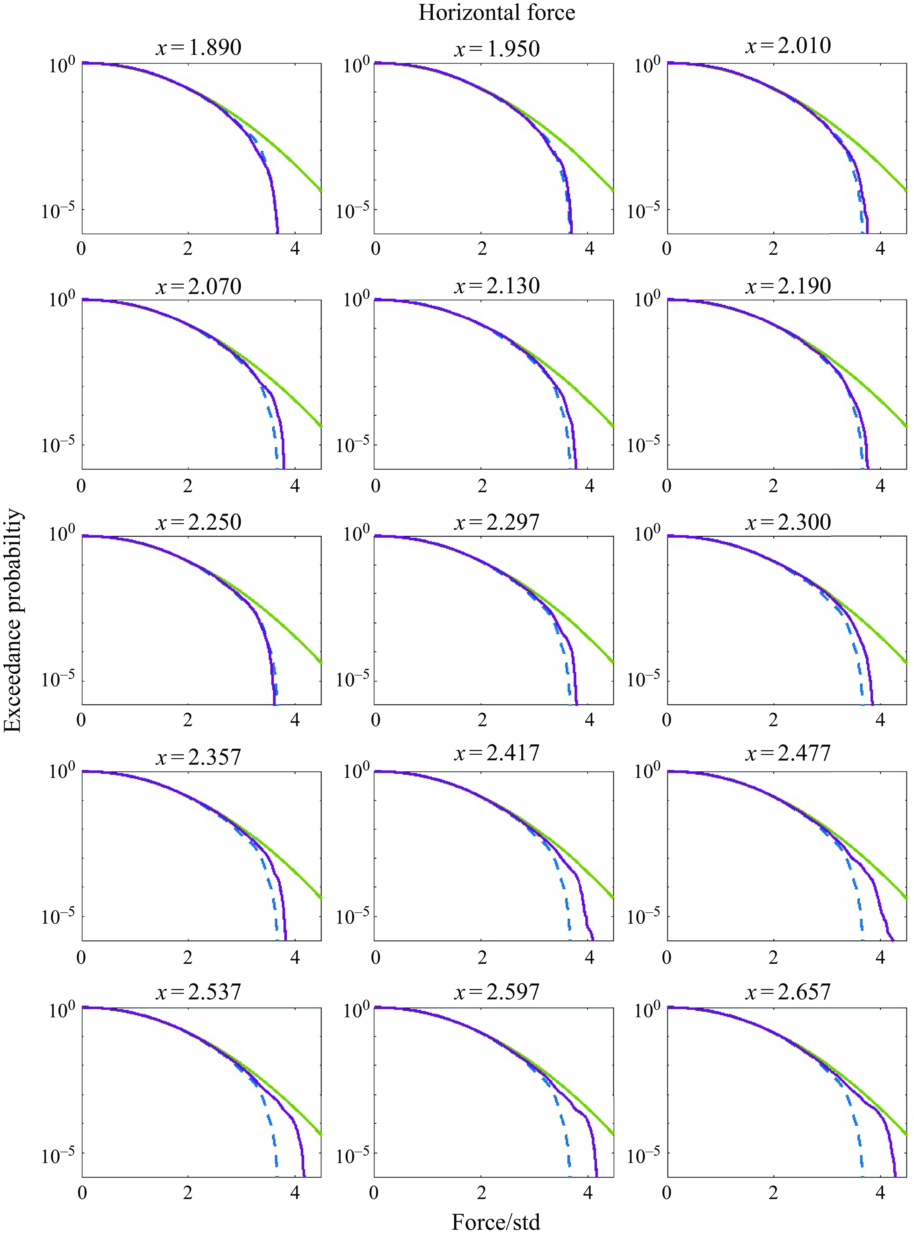
Figure 12. Exceedance probability of the Hilbert envelope of the horizontal force normalized by its standard deviation. With shoal indicated by purple; reference measurement without shoal indicated by dashed blue; Rayleigh distribution indicated by green.
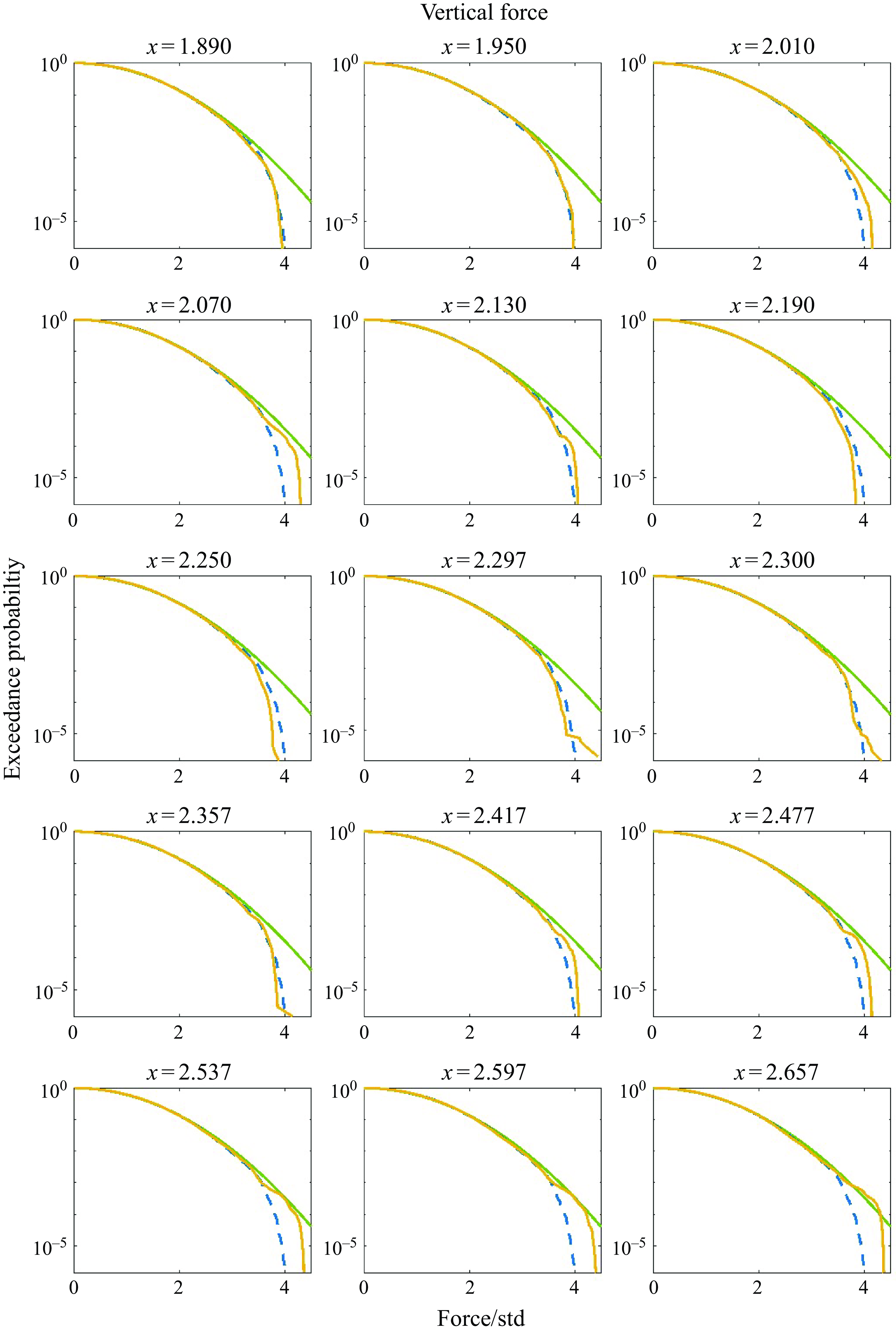
Figure 13. Same as in figure 12, but for vertical force (yellow).
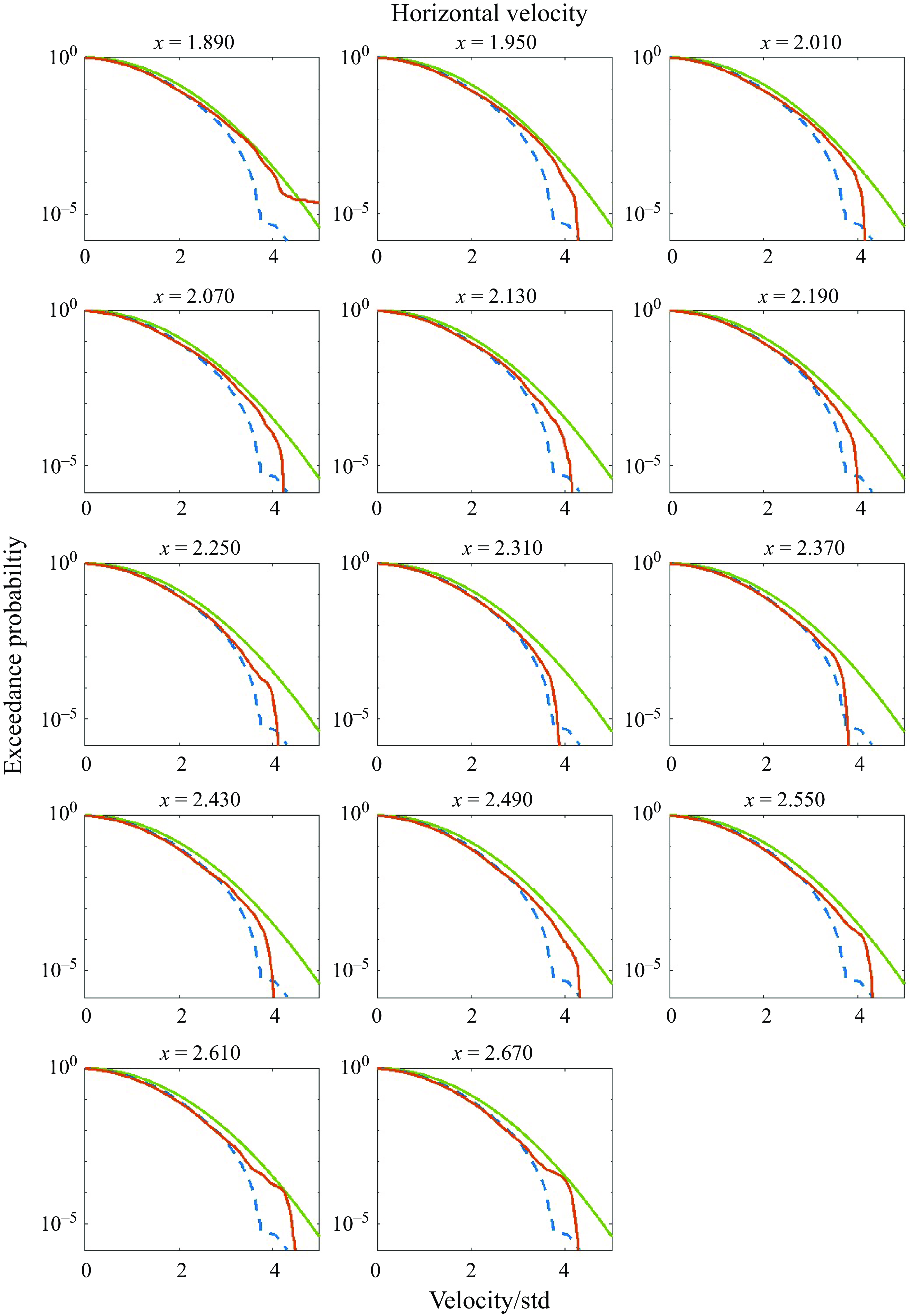
Figure 14. Same as in figure 12, but for horizontal velocity (orange).
4.3. Exceedance probability of the Hilbert envelope
In figures 12, 13 and 14, the exceedance probability of the Hilbert envelope of the force and velocity measurements is presented, normalized by the standard deviation of the measurements at the same position. This is compared to the measurements over the flat bottom and the Rayleigh distribution.
From figure 12, it can be seen that the exceedance probability distribution for the Hilbert envelope of the horizontal force over the shoal is not following the Rayleigh distribution for the largest forces, but as the water depth increases, it comes closer to it. Also, as the water depth increases, the exceedance probability for large forces is higher for the measurements over the shoal compared to measurements over the flat bottom.
The exceedance probability for the vertical force, shown in figure 13, is closer to the Rayleigh distribution than for the horizontal force, and has a higher probability than the Rayleigh distribution for the largest forces at the last position.
A similar trend as for the vertical force is happening for the horizontal velocity, with exceedance probability shown in figure 14. However, for the velocity, the distribution is below the Rayleigh distribution for the small forces as well as for the large ones, and at all positions.
From these figures of the exceedance probability of the Hilbert envelope, we therefore see that the measurements for forces and velocity give distributions close to, but not equal to, the Rayleigh distribution.
5. Conclusion
We have found that the presence of a shoal can modify the statistical distribution of a wave field, with respect to surface elevation field, velocity field, acceleration field and the forces experienced on a horizontal cylinder in the vicinity of the shoal. For surface elevation, horizontal velocity and horizontal acceleration, our results reproduce the behaviour in skewness and kurtosis observed in earlier research. A submerged horizontal cylinder can experience forces with increased values of skewness and kurtosis and a modified statistical force distribution with thicker extreme tails, when it is over the down-slope of a shoal compared to over a flat bottom. For the shapes of the probability distributions of the horizontal force, the spatial dependence evolves in a more similar way to the acceleration than to the velocity along the down-slope of the shoal, as could be expected for an inertia-dominated regime. However, the spatial dependence of the skewness and kurtosis is different between surface elevation, velocity field, acceleration field and the forces experienced by a submerged horizontal cylinder.
Acknowledgements.
We thank O. Gundersen for building and installing the experimental set-up. The force transducers were provided by SINTEF Ocean.
Declaration of interests.
The authors report no conflict of interest.


 Open access