


1. Introduction
The potential of wave energy as a renewable electricity source has been assessed to exceed the global demand for electricity (Sheng Reference Sheng2019; Mork et al. Reference Mork, Barstow, Kabuth and Pontes2010). However, efficient designs still remain to be developed at an industrial level. Horizontally submerged flexible plates could be part of those designs due to their improved survivability (Collins et al. Reference Collins, Hossain, Dettmer and Masters2021). Until now, flexible submerged elastic plates have mostly been studied numerically and theoretically in a configuration where both edges are clamped, with the objective of harnessing wave energy or protecting the coastline. Cho & Kim (Reference Cho and Kim1998) and Cho & Kim (Reference Cho and Kim2000) considered the plate as a potential wave barrier. From the on-site observations that a muddy seafloor can effectively dampen water waves, Alam (Reference Alam2012) proposed a design to harvest wave energy by mimicking this phenomenon. To that aim, a flexible plate is used as a wave energy harvester. The flexible plate is hinged at the seafloor and oscillates due to the wave forcing, similarly to the mud in the ocean floor. Those oscillations are used to produce electricity by means of a power take-off (PTO) system. The Wave-Carpet design has been investigated numerically and experimentally by Desmars et al. (Reference Desmars, Tchoufag, Younesian and Alam2018), Asaeian et al. (Reference Asaeian, Abedi, Jafari-Talookolaei and Attar2020) and Lehmann et al. (Reference Lehmann, Elandt, Pham, Ghorbani, Shakeri and Alam2013). Renzi (Reference Renzi2016) studied numerically a variation of the Wave-Carpet considering the use of a piezoelectric material to produce electricity, while Achour et al. (Reference Achour, Mougel, Lo Jacono and Fabre2020) added the effect of a current in addition to the waves. Boral et al. (Reference Boral, Sahoo and Meylan2023) investigated the case of a flexible thin submerged plate resting on an elastic foundation modelled using the Winkler approach. Finally, submerged flexible plates clamped at both edges have been studied in more complex configurations, such as close to a wall as potential wave barriers (Guo et al. Reference Guo, Mohapatra and Soares2020; Gayathri et al. Reference Gayathri, Benny and Behera2020; Mohapatra & Guedes Soares Reference Mohapatra and Guedes Soares2020), superimposed with other plates (Mohapatra & Sahoo Reference Mohapatra and Sahoo2014; Mohapatra & Guedes Soares Reference Mohapatra and Guedes Soares2019; Behera Reference Behera2021; Das et al. Reference Das, Sahoo and Meylan2020) or in series (Mirza & Hassan Reference Mirza and Hassan2024 Reference Mirza and Hassan a ,Reference Mirza and Hassan b ).
Contrary to the two-edge clamping, clamping the plate at only one edge has barely been studied. Shoele (Reference Shoele2023) investigated numerically the case of a submerged elastic plate as a hybrid current/wave energy converter but the impact of waves alone was not examined. Michele et al. (Reference Michele, Buriani, Renzi, van Rooij, Jayawardhana and Vakis2020) investigated the behaviour of a floating elastic plate moored onto a set of PTO systems. Their theoretical model shows that plate elasticity introduces additional resonant frequencies compared with rigid plates, enhancing both wave energy extraction and the capture factor bandwidth. While their preliminary experimental estimations of power extraction with a flexible floater demonstrator compared favourably with their model, the wave–structure interaction mechanisms remain largely unexplored.
The aim of this paper is to characterize experimentally the interaction of a flexible submerged elastic plate, clamped at only one edge, with water waves. A table-top experiment has been developed to study the wave–plate interaction, which allows the use of vision-based data extraction techniques. Schlieren imaging is utilized to measure the free-surface height and a side view of the tank to track the plate deformation. The ability of the plate to reflect, transmit or dissipate water waves is computed measuring the reflection and transmission coefficients. It is observed that the flexible plate can reflect water waves over a certain range of waves frequencies. It exposes potential applications of such a system for coastal protection and, more generally, offers a deeper fundamental understanding of the role played by flexibility in the wave–structure interaction applications. The comparison of wave reflection and transmission by a submerged flexible plate and a submerged rigid plate of the same dimensions shows that the plate motion is responsible for wave reflection. Finally, when increasing the wave amplitude, the flexible plate can act like a perfect wave absorber by changing its mean position. The flexible plate acts as a reconfigurable water-wave absorber which could be able to totally dampen the waves in high sea conditions.
2. Experimental methods

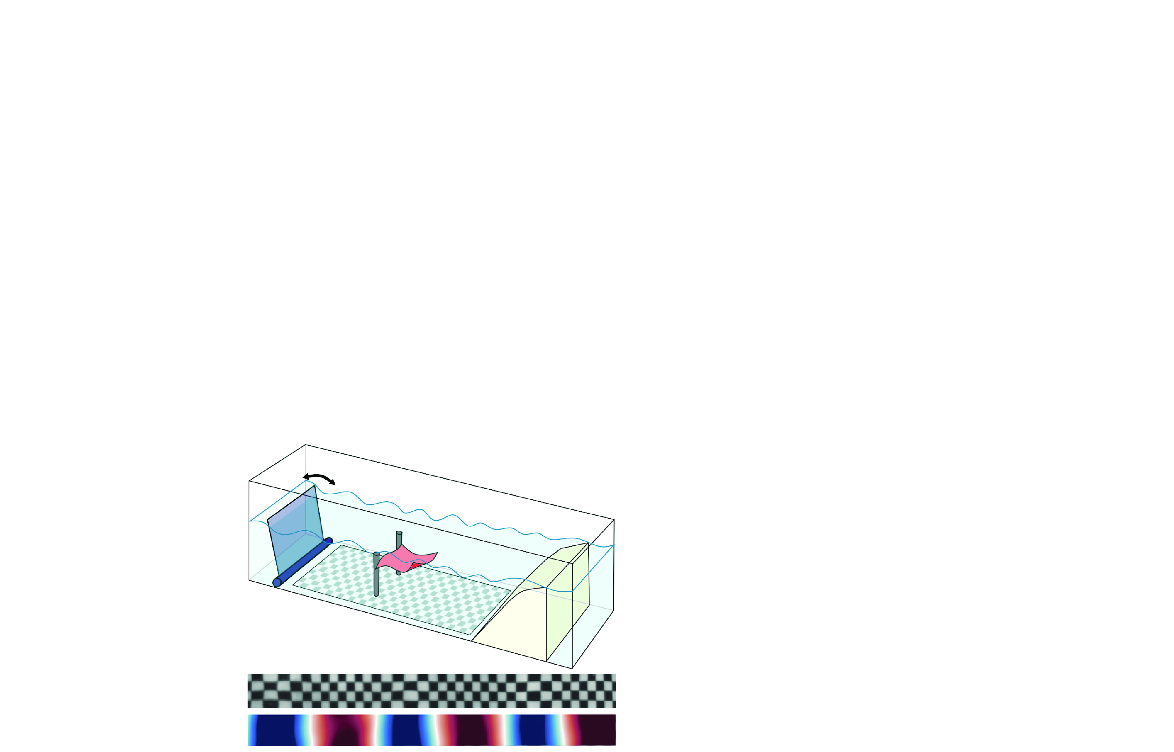
Figure 1. (a) Schematic diagram of the experimental set-up. The plate length
 $L$
is 28 cm. (b) Side view of the tank with the plate: picture (I) is a raw image while picture (II) illustrates the detected edge of the plate (red line). (c) Tank top view: picture (I) is taken with an undisturbed free surface. For picture (II), 3.5 Hz/13 cm waves of 3 mm amplitude are generated and the chequerboard appears deformed. The bottom picture illustrates the free-surface height reconstruction using Schlieren imaging.
$L$
is 28 cm. (b) Side view of the tank with the plate: picture (I) is a raw image while picture (II) illustrates the detected edge of the plate (red line). (c) Tank top view: picture (I) is taken with an undisturbed free surface. For picture (II), 3.5 Hz/13 cm waves of 3 mm amplitude are generated and the chequerboard appears deformed. The bottom picture illustrates the free-surface height reconstruction using Schlieren imaging.
2.1. Experimental set-up
The experimental set-up is represented in figure 1(a), in a reference frame with
 $x$
the direction of propagation of the waves,
$x$
the direction of propagation of the waves,
 $y$
the transverse direction, and
$y$
the transverse direction, and
 $z$
the vertical coordinate, respectively. The total length of the tank is 2.5 m, where the measurement region is 2 m long at the centre of the tank. The tank width is restricted to a 12 cm channel to prevent transverse modes in the investigated range of frequencies (Ursell Reference Ursell1952). Water depth is fixed at 10 cm. Waves are produced using a flap type wave-maker driven by a linear motor (DM 01-23x80F-HP-R-60_MS11 from Linmot®). In practice, the waves produced in this set-up have an amplitude ranging from 0.5 to 5 mm and frequencies ranging from 1.5 to 4 Hz. The wave angular frequency,
$z$
the vertical coordinate, respectively. The total length of the tank is 2.5 m, where the measurement region is 2 m long at the centre of the tank. The tank width is restricted to a 12 cm channel to prevent transverse modes in the investigated range of frequencies (Ursell Reference Ursell1952). Water depth is fixed at 10 cm. Waves are produced using a flap type wave-maker driven by a linear motor (DM 01-23x80F-HP-R-60_MS11 from Linmot®). In practice, the waves produced in this set-up have an amplitude ranging from 0.5 to 5 mm and frequencies ranging from 1.5 to 4 Hz. The wave angular frequency,
 $\omega$
, is related to the wavenumber,
$\omega$
, is related to the wavenumber,
 $k$
, through the dispersion relation of gravity waves:
$k$
, through the dispersion relation of gravity waves:
 \begin{equation} \omega ^2=gk\tanh (kh), \end{equation}
where
 $g$
is the acceleration of gravity and
$g$
is the acceleration of gravity and
 $h$
the water depth. The studied wavelengths,
$h$
the water depth. The studied wavelengths,
 $\lambda$
, range from 10 to 55 cm, so that
$\lambda$
, range from 10 to 55 cm, so that
 $\lambda /h$
ranges from 1 to 5.5, corresponding to deep to intermediate water depths. The plate is positioned halfway through the tank length at
$\lambda /h$
ranges from 1 to 5.5, corresponding to deep to intermediate water depths. The plate is positioned halfway through the tank length at
 $x=0$
m. At the end of the tank, a parabolic beach is placed. It is used to limit reflection on the tank wall (Ouellet & Datta Reference Ouellet and Datta1986). The beach is pierced with 5 mm circular holes to enhance viscous damping. Data are extracted from this set-up by filming simultaneously from the top and the side of the tank, giving access to the free-surface deformation and the plate motion.
$x=0$
m. At the end of the tank, a parabolic beach is placed. It is used to limit reflection on the tank wall (Ouellet & Datta Reference Ouellet and Datta1986). The beach is pierced with 5 mm circular holes to enhance viscous damping. Data are extracted from this set-up by filming simultaneously from the top and the side of the tank, giving access to the free-surface deformation and the plate motion.
2.2. Water-wave height measurements
The free-surface deformation is computed using Schlieren imaging (Moisy et al. Reference Moisy, Rabaud and Salsac2009; Wildeman Reference Wildeman2018). To do so, a chequerboard pattern is placed at the bottom of the tank. When waves propagate, the image of the chequerboard obtained by filming with the top camera appears to be deformed, as illustrated in figure 1(c). Both figures 1(c) (I) and (II) show an image taken by the top camera with the plate placed in the middle of the tank. In (I), no waves are propagating, whereas in (II) 3.5 Hz/13 cm waves of 2.5 mm amplitude are propagating in the tank. The comparison between those two images is used to reconstruct the free-surface height in all the tank by using the open-source code provided by Wildeman (Reference Wildeman2018). Figure 1
(c) (III) illustrates free-surface reconstruction using images (I) and (II). The tank can be divided into two different regions: the up-wave region, located between the wave-maker and the plate, where the incoming wave, produced by the wave-maker, and the wave reflected by the plate propagate; and the down-wave region, located between the plate and the beach, where waves transmitted by the plate propagate, as well as a small component of waves reflected from the absorption beach. After filtering at the wave-maker angular frequency,
 $\omega$
, the free-surface elevation can be described as the sum of two waves propagating forward and backward in each region:
$\omega$
, the free-surface elevation can be described as the sum of two waves propagating forward and backward in each region:
 \begin{equation} \left \{ \begin{array}{lll} \eta ^{uw}(x,t)=\mathrm {Re}(\hat \eta ^{uw}_+(x)e^{-i\omega t}+\hat \eta ^{uw}_-(x)e^{-i\omega t})\,\,\mathrm {with}\,\, \hat \eta ^{uw}_\pm (x)=\hat A_\pm ^{uw}e^{\pm (ik-\nu )x }\\ \\ \eta ^{dw}(x,t)=\mathrm {Re}(\hat \eta ^{dw}_+(x)e^{-i\omega t}+\hat \eta ^{dw}_-(x)e^{-i\omega t})\,\,\mathrm {with}\,\, \hat \eta ^{dw}_\pm (x)=\hat A_\pm ^{dw}e^{\pm (ik-\nu )x },\\ \end{array} \right . \end{equation}
where
 $\eta$
is the free-surface height and the superscripts uw and dw stand for up-wave and down-wave, respectively. Quantities associated with waves propagating forward and downward are indicated using the subscripts + and −, respectively, and complex numbers are denoted using the symbol
$\eta$
is the free-surface height and the superscripts uw and dw stand for up-wave and down-wave, respectively. Quantities associated with waves propagating forward and downward are indicated using the subscripts + and −, respectively, and complex numbers are denoted using the symbol
 $\;\hat{}\,$
. Here
$\;\hat{}\,$
. Here
 $\hat \eta$
is the complex spatial part of the free-surface height (it depends on
$\hat \eta$
is the complex spatial part of the free-surface height (it depends on
 $k$
the wavenumber),
$k$
the wavenumber),
 $\hat A$
the complex wave amplitudes, and
$\hat A$
the complex wave amplitudes, and
 $\nu$
a damping coefficient that models wave dissipation along the tank.
$\nu$
a damping coefficient that models wave dissipation along the tank.
The energy reflection and transmission coefficients,
 $K_r$
and
$K_r$
and
 $K_t$
, for a given wave amplitude and frequency are defined as
$K_t$
, for a given wave amplitude and frequency are defined as
 \begin{equation} K_r=\left (\frac {|\hat A_-^{uw}|}{|\hat A_+^{uw}|}\right )^2\,\mathrm {and}\,K_t=\left (\frac {|\hat A_+^{dw}|}{|\hat A_+^{uw}|}\right )^2. \end{equation}
To determine the reflection and transmission coefficients, the amplitude of the waves propagating forward and backward have to be measured.The image deformation is related to the free-surface height by (Moisy et al. Reference Moisy, Rabaud and Salsac2009)
 \begin{equation} \nabla \eta =-\frac {\boldsymbol{u}}{h^*}, \end{equation}
where
 $h^*$
is a real-valued parameter that depends on water depth and set-up configuration and
$h^*$
is a real-valued parameter that depends on water depth and set-up configuration and
 $\boldsymbol{u}$
is the deformation field. The vector
$\boldsymbol{u}$
is the deformation field. The vector
 $\boldsymbol{u}$
has two components,
$\boldsymbol{u}$
has two components,
 $u_x$
and
$u_x$
and
 $u_y$
, corresponding to the image deformation along
$u_y$
, corresponding to the image deformation along
 $x$
and
$x$
and
 $y$
. Generally,
$y$
. Generally,
 $\eta$
is obtained by numerically inverting the gradient. However, as the free-surface height is non-zero on the edges of the image, the determination of the integration constant leads to numerical errors. In this work, gradient inversion is avoided by using the monochromatic nature of the waves studied. The elevation gradient,
$\eta$
is obtained by numerically inverting the gradient. However, as the free-surface height is non-zero on the edges of the image, the determination of the integration constant leads to numerical errors. In this work, gradient inversion is avoided by using the monochromatic nature of the waves studied. The elevation gradient,
 $\nabla \hat \eta$
, is reduced to a simple partial derivative along
$\nabla \hat \eta$
, is reduced to a simple partial derivative along
 $x$
. Equation 2.2, leads to
$x$
. Equation 2.2, leads to
 \begin{equation} \nabla \hat \eta _+=(ik-\nu )\hat \eta _+\,\,\mathrm {and}\,\,\nabla \hat \eta _-=-(ik-\nu )\hat \eta _-. \end{equation}
The Fourier transform of
 $u_x$
at the wave-maker frequency,
$u_x$
at the wave-maker frequency,
 $\hat u_x(x)$
, can also be decomposed in its forward/backward components as
$\hat u_x(x)$
, can also be decomposed in its forward/backward components as
 \begin{equation} \hat u_x(x)=\hat u_{x+}e^{(ik-\nu )x}+\hat u_{x-}e^{(-ik+\nu )x}, \end{equation}
with
 \begin{equation} \hat u_{x+}=-(ik-\nu )h^*\hat \eta _+\,\,\mathrm {and}\,\,\hat u_{x-}=(ik-\nu )h^*\hat \eta _-. \end{equation}
Therefore, for monochromatic waves,
 $K_r$
and
$K_r$
and
 $K_t$
can be computed using only the image deformation:
$K_t$
can be computed using only the image deformation:
 \begin{equation} K_r=\left (\frac {|\hat u_{x-}^{uw}|}{|\hat u_{x+}^{uw}|}\right )^2\,\mathrm {and}\,K_t=\left (\frac {|\hat u_{x+}^{dw}|}{|\hat u_{x+}^{uw}|}\right )^2. \end{equation}
The four deformation amplitudes are obtained by choosing an arbitrary set of positions
 $x_i$
where
$x_i$
where
 $\hat u_x$
is evaluated. The different amplitudes and the damping coefficient are determined by solving the system
$\hat u_x$
is evaluated. The different amplitudes and the damping coefficient are determined by solving the system
 \begin{equation} \left \{ \begin{array}{lll} \hat u_x(x_1)=\hat u_{x+}\exp (ikx_1-\nu x_1)+\hat u_{x-}\exp (-ikx_1+\nu x_1)\\ \vdots \\ \hat u_x(x_{\mathrm {max}})=\hat u_{x+}\exp (ikx_{\mathrm {max}}-\nu x_{\mathrm {max}})+\hat u_{x-}\exp (-ikx_{\mathrm {max}}+\nu x_{\mathrm {max}}), \end{array} \right . \end{equation}
using a nonlinear least-squares method.
Top- and side-view movies are taken simultaneously by following the same protocol. First, a picture of the undisturbed tank is taken, giving a reference image for the top and side view. Then waves are sent for one minute and fifteen seconds. The first minute is used to reach a steady state and data are acquired during the last 15 s.
2.3. Plate characteristics and clamping system
The plate is placed submerged as pictured in figure 1, at a fixed depth of 3 cm. The leading edge of the plate is maintained submerged using a clamping system composed of two carbon rods of 2 mm diameter that are glued to the edge of the plate. The rods are attached to the support poles on the sides of the tank, ensuring that the leading edge remains still. The plate material choice is particularly crucial. Indeed, since the plate trailing edge remains free, a small density difference with water will induce a deviation from the horizontal at rest. In practice, such deviation can be mitigated by using a relatively rigid material. The plate itself is made by cutting polypropylene sheets of density 1035 kg m
 $^{-3}$
and stiffness 1.7 × 10
$^{-3}$
and stiffness 1.7 × 10
 $^{-3}$
N m
$^{-3}$
N m
 $^{2}$
.
$^{2}$
.
Figure 1(b) (I) is taken from the tank side view and shows the plate when no waves are present. The plate edge is coloured in black to allow its tracking as illustrated in picture (II). As can be appreciated, the plate position is close to horizontal. The plate length,
 $L$
, is fixed at 28 cm, which enables the testing of ratios
$L$
, is fixed at 28 cm, which enables the testing of ratios
 $L/\lambda$
ranging from 0.45 to
2.7. The plate resonance frequencies have been measured forcing the plate at a 3 cm depth. For forcing frequencies between 0.5 and 4 Hz, two resonance frequencies of the system are observed, corresponding to the second and third plate mode, at respectively
$L/\lambda$
ranging from 0.45 to
2.7. The plate resonance frequencies have been measured forcing the plate at a 3 cm depth. For forcing frequencies between 0.5 and 4 Hz, two resonance frequencies of the system are observed, corresponding to the second and third plate mode, at respectively
 $f_2=0.6$
Hz and
$f_2=0.6$
Hz and
 $f_3=1.96$
Hz.
$f_3=1.96$
Hz.

Figure 2. (a) Average over three experiments of the reflection and transmission coefficients,
 $K_r$
(blue squares) and
$K_r$
(blue squares) and
 $K_t$
(red triangles) for
$K_t$
(red triangles) for
 $L/\lambda$
from 0.45 to 2.7. A significant reflection is observed for
$L/\lambda$
from 0.45 to 2.7. A significant reflection is observed for
 $L/\lambda$
between 0.6 and 1.6 while for other values the plate mostly transmits waves. (b) Plate deflection
$L/\lambda$
between 0.6 and 1.6 while for other values the plate mostly transmits waves. (b) Plate deflection
 $w$
normalized by the incoming wave amplitude,
$w$
normalized by the incoming wave amplitude,
 $A$
, for six values of
$A$
, for six values of
 $L/\lambda$
indicated by I to VI in (a). Across the different values of
$L/\lambda$
indicated by I to VI in (a). Across the different values of
 $L/\lambda$
, the plate amplitude of motion decreases and its deformation mode changes. (c) Reflection (blue squares) and transmission (red triangles) coefficients for a rigid plate of same dimensions as the flexible one. No reflection is observed, underlining the fact that the wave reflection is induced by the plate motion.
$L/\lambda$
, the plate amplitude of motion decreases and its deformation mode changes. (c) Reflection (blue squares) and transmission (red triangles) coefficients for a rigid plate of same dimensions as the flexible one. No reflection is observed, underlining the fact that the wave reflection is induced by the plate motion.
3. Results
3.1. Low-wave-amplitude forcing
Figure 2(a) shows the average, over three experiments, of the reflection and transmission coefficients,
 $K_r$
and
$K_r$
and
 $K_t$
, measured as a function of the ratio
$K_t$
, measured as a function of the ratio
 $L/\lambda$
. These experiments were conducted with a water-wave amplitude of approximately 0.5 mm, which corresponds to the lowest wave amplitude that can be produced and effectively analysed. At lower values of
$L/\lambda$
. These experiments were conducted with a water-wave amplitude of approximately 0.5 mm, which corresponds to the lowest wave amplitude that can be produced and effectively analysed. At lower values of
 $L/\lambda$
, waves are mostly transmitted by the plate with the reflection coefficient,
$L/\lambda$
, waves are mostly transmitted by the plate with the reflection coefficient,
 $K_r$
, being almost equal to 0 for point (I). Increasing
$K_r$
, being almost equal to 0 for point (I). Increasing
 $L/\lambda$
leads
$L/\lambda$
leads
 $K_t$
to drop to 0 and
$K_t$
to drop to 0 and
 $K_r$
to rise to 60 % of the incoming wave energy (IV). For
$K_r$
to rise to 60 % of the incoming wave energy (IV). For
 $L/\lambda$
larger than 1.6,
$L/\lambda$
larger than 1.6,
 $K_r$
drops again to 0 and the plate mostly transmits waves. It is observed that for
$K_r$
drops again to 0 and the plate mostly transmits waves. It is observed that for
 $L/\lambda \lt 1.6$
,
$L/\lambda \lt 1.6$
,
 $K_r+K_t\lt 1$
, implying that a significant part of the incoming wave energy is dissipated. Figure 2(b) shows the plate deflection over one wave period, normalized by the incoming wave amplitude for different values of
$K_r+K_t\lt 1$
, implying that a significant part of the incoming wave energy is dissipated. Figure 2(b) shows the plate deflection over one wave period, normalized by the incoming wave amplitude for different values of
 $L/\lambda$
. When increasing
$L/\lambda$
. When increasing
 $L/\lambda$
, the plate amplitude of motion decreases. Also, when
$L/\lambda$
, the plate amplitude of motion decreases. Also, when
 $L/\lambda$
increases, the plate changes its deformation mode. It is illustrated by figure 2(b) (I) and (II) that have one node, while (III) and (IV) show two nodes. As illustrated by cases (V) and (VI), the values of
$L/\lambda$
increases, the plate changes its deformation mode. It is illustrated by figure 2(b) (I) and (II) that have one node, while (III) and (IV) show two nodes. As illustrated by cases (V) and (VI), the values of
 $L/\lambda$
, where the plate fully transmits water waves, is associated with almost no plate motion.
$L/\lambda$
, where the plate fully transmits water waves, is associated with almost no plate motion.
The reflection and transmission are also examined using a rigid plate made of aluminium having the same dimensions as the flexible plate. The corresponding
 $K_r$
and
$K_r$
and
 $K_t$
are presented in figure 2(c) as a function of
$K_t$
are presented in figure 2(c) as a function of
 $L/\lambda$
. No reflection pattern is observed using a rigid plate, highlighting the fact that the plate motion is necessary to reflect water waves in this case.
$L/\lambda$
. No reflection pattern is observed using a rigid plate, highlighting the fact that the plate motion is necessary to reflect water waves in this case.
From a frequency perspective, the reflection zone is centred on 2.5 Hz (i.e.
 $f/f_2=4$
and
$f/f_2=4$
and
 $f/f_3=1.25$
), covering frequencies between 1.8 and 3 Hz (i.e.
$f/f_3=1.25$
), covering frequencies between 1.8 and 3 Hz (i.e.
 $f/f_2\in[ 3-5]$
and
$f/f_2\in[ 3-5]$
and
 $f/f_3\in[ 0.9-1.5]$
).
$f/f_3\in[ 0.9-1.5]$
).
3.2. Large-wave-amplitude forcing
Figures 3(a) and 3(b) illustrate the influence of the incoming wave amplitude,
 $A_+$
, on the transmission and reflection coefficients, respectively. At lower
$A_+$
, on the transmission and reflection coefficients, respectively. At lower
 $L/\lambda$
, the wave amplitude has no influence on wave transmission by the plate. However, for larger
$L/\lambda$
, the wave amplitude has no influence on wave transmission by the plate. However, for larger
 $L/\lambda$
, a drop in transmission is observed when
$L/\lambda$
, a drop in transmission is observed when
 $A_+$
increases. In terms of reflection, the increase in the incoming wave amplitude leads to an attenuation of the reflection peak. By interpolating all the experimental data points, we produce both the
$A_+$
increases. In terms of reflection, the increase in the incoming wave amplitude leads to an attenuation of the reflection peak. By interpolating all the experimental data points, we produce both the
 $K_r$
and
$K_r$
and
 $K_t$
maps in a wave-amplitude-
$K_t$
maps in a wave-amplitude-
 $L/\lambda$
space shown in figures 3(c) and 3(d). The lower amplitude case corresponds to data presented in § 3.1 with significant reflection for
$L/\lambda$
space shown in figures 3(c) and 3(d). The lower amplitude case corresponds to data presented in § 3.1 with significant reflection for
 $L/\lambda$
between 0.6 and 1.6. When increasing the wave amplitude, the reflection and transmission patterns are drastically modified. For
$L/\lambda$
between 0.6 and 1.6. When increasing the wave amplitude, the reflection and transmission patterns are drastically modified. For
 $A_+\gt 3$
mm, waves are neither reflected nor transmitted for
$A_+\gt 3$
mm, waves are neither reflected nor transmitted for
 $L/\lambda \gt 0.6$
, meaning that the incoming wave energy is totally dissipated when interacting with the plate. This dissipation can be attributed to a change in the plate mean position for the
$L/\lambda \gt 0.6$
, meaning that the incoming wave energy is totally dissipated when interacting with the plate. This dissipation can be attributed to a change in the plate mean position for the
 $(A_+,L/\lambda )$
couples that are illustrated in figure 3. Figure 4(a) shows a picture taken from the side of the tank when conducting experiments for
$(A_+,L/\lambda )$
couples that are illustrated in figure 3. Figure 4(a) shows a picture taken from the side of the tank when conducting experiments for
 $A_+=6$
mm and
$A_+=6$
mm and
 $L/\lambda =0.99$
. The plate tip reaches the free surface under the effect of the waves. Similarly to a beach, this configuration is found to be particularly efficient to break water waves. The change in plate tip mean position,
$L/\lambda =0.99$
. The plate tip reaches the free surface under the effect of the waves. Similarly to a beach, this configuration is found to be particularly efficient to break water waves. The change in plate tip mean position,
 $\Delta _i$
, can be measured for all the experiments. Its values are presented in figure 4(b). The region where both
$\Delta _i$
, can be measured for all the experiments. Its values are presented in figure 4(b). The region where both
 $K_r$
and
$K_r$
and
 $K_t$
are equal to 0 corresponds to
$K_t$
are equal to 0 corresponds to
 $\Delta _i/d\approx1$
, i.e. experiments for which the plate tip reaches the free surface. Figure 4(c) illustrates the correlation between the plate tip position and the part of the incoming wave energy that is dissipated,
$\Delta _i/d\approx1$
, i.e. experiments for which the plate tip reaches the free surface. Figure 4(c) illustrates the correlation between the plate tip position and the part of the incoming wave energy that is dissipated,
 $1-K_r-K_t$
. The region where the plate tip reaches the free surface corresponds to the region where all the energy of the incoming wave is dissipated because of the interaction with the plate,
i.e.
$1-K_r-K_t$
. The region where the plate tip reaches the free surface corresponds to the region where all the energy of the incoming wave is dissipated because of the interaction with the plate,
i.e.
 $1-K_r-K_t=1$
. For higher
$1-K_r-K_t=1$
. For higher
 $L/\lambda$
and lower amplitudes, no energy is dissipated, which is associated with regimes where the plate does not move.
$L/\lambda$
and lower amplitudes, no energy is dissipated, which is associated with regimes where the plate does not move.

Figure 3. (a) Transmission coefficient,
 $K_t$
, as a function of
$K_t$
, as a function of
 $L/\lambda$
for six different wave amplitudes. The wave amplitude is indicated with different colours, from black to yellow, yellow corresponding to higher wave amplitudes. At low
$L/\lambda$
for six different wave amplitudes. The wave amplitude is indicated with different colours, from black to yellow, yellow corresponding to higher wave amplitudes. At low
 $L/\lambda$
, the wave amplitude has a lower impact on
$L/\lambda$
, the wave amplitude has a lower impact on
 $K_t$
, while for high-amplitude waves, the transmission coefficient drops to zero. (b) Reflection coefficient,
$K_t$
, while for high-amplitude waves, the transmission coefficient drops to zero. (b) Reflection coefficient,
 $K_r$
, as a function of
$K_r$
, as a function of
 $L/\lambda$
for six different wave amplitudes, using the same colour code as for the transmission coefficient. The increase in wave amplitude leads to a decrease in transmission. (c,d) The
$L/\lambda$
for six different wave amplitudes, using the same colour code as for the transmission coefficient. The increase in wave amplitude leads to a decrease in transmission. (c,d) The
 $A \rm vs L/\lambda$
diagrams showing the transmission (c) and reflection coefficients (d) interpolated using experimental data to cover the whole domain. Bright colours correspond to the coefficient being equal to 0 and dark colours to the coefficient equal to 1. For the steepest waves, no reflection and no transmission are observed, meaning that the plate dissipates all the incoming wave energy.
$A \rm vs L/\lambda$
diagrams showing the transmission (c) and reflection coefficients (d) interpolated using experimental data to cover the whole domain. Bright colours correspond to the coefficient being equal to 0 and dark colours to the coefficient equal to 1. For the steepest waves, no reflection and no transmission are observed, meaning that the plate dissipates all the incoming wave energy.

Figure 4. (a) Side view of the tank while sending waves of 6 mm amplitude with
 $L/\lambda=0.99$
. The plate tip is displaced from its initial position of
$L/\lambda=0.99$
. The plate tip is displaced from its initial position of
 $\Delta _i$
and reaches the free surface. (b) Plate tip mean displacement
$\Delta _i$
and reaches the free surface. (b) Plate tip mean displacement
 $\Delta _i$
normalized by plate depth
$\Delta _i$
normalized by plate depth
 $d$
in an
$d$
in an
 $A_+$
vs
$A_+$
vs
 $L/\lambda$
map. For the steepest waves,
$L/\lambda$
map. For the steepest waves,
 $\Delta _i\approx d$
, meaning that the plate tip reaches the free surface. (c) The
$\Delta _i\approx d$
, meaning that the plate tip reaches the free surface. (c) The
 $A_+$
vs
$A_+$
vs
 $L/\lambda$
map of
$L/\lambda$
map of
 $1-K_r-K_t$
, meaning the part of the incoming wave energy that is dissipated by the interaction with the plate. Dissipation is maximum for the steepest waves.
$1-K_r-K_t$
, meaning the part of the incoming wave energy that is dissipated by the interaction with the plate. Dissipation is maximum for the steepest waves.
4. Discussion and conclusion
The present study characterizes the interaction between a flexible plate, clamped at one edge, with water waves. It highlights experimentally that in such a configuration, the flexible plate can reflect wave energy. The comparison with a rigid plate enlightens the key role played by the plate’s flexibility for potential coastal protection applications. The role of flexibility in structures intended for coastal protection has been largely discussed and is known to enhance wave dissipation compared with rigid structures (Kumar et al. Reference Kumar, Manam and Sahoo2007). However, the influence of flexibility on wave reflection remains generally unclear. For instance, Stamos & Hajj (Reference Stamos and Hajj2001) reported higher reflection coefficients for rigid submerged breakwaters. The present work highlights the opposite behaviour for a submerged elastic plate.
For this system, an uncommon physical process enhances wave dissipation. Owing to its ability to change its mean position when forced by the waves, the plate is passively placed in a configuration extremely efficient to break water waves. This configuration change, where the plate tip reaches the free surface, intervenes for the steepest water waves. The minimal steepness at which a significant change in position occurs is
 $A_+/\lambda \approx 10^{-2}$
, for
$A_+/\lambda \approx 10^{-2}$
, for
 $A_+=3$
mm and
$A_+=3$
mm and
 $L/\lambda \approx 1$
, which corresponds to slightly nonlinear waves (Le Méhauté Reference Le Méhauté1976). Strong nonlinear behaviours can therefore be observed for waves that are far from the breaking limit. Several phenomena could be responsible for the plate changing its mean position. First, if a current takes place between the plate and the free surface, it could cause a depression similar to a Venturi effect. In such a configuration, Stokes drift could arise from wave steepness (Stokes Reference Stokes1847; Van den Bremer & Breivik Reference Van den Bremer and Breivik2018). In addition, waves above a rigid plate can lead to the creation of a mean flow (Carmigniani et al. Reference Carmigniani, Benoit, Violeau and Gharib2017). The flow at the edge of the plate could explain the observations through its associated upward force. In the case of a rigid plate in a wave field, vortex creation has been reported by Boulier & Belorgey (Reference Boulier and Belorgey1994), Poupardin et al. (Reference Poupardin, Perret, Pinon, Bourneton, Rivoalen and Brossard2012) and Pinon et al. (Reference Pinon, Perret, Cao, Poupardin, Brossard and Rivoalen2017). They observed that the vortex street has a given direction, slightly upward or downward. A similar phenomenon could exert a force upward on the plate tip.
$L/\lambda \approx 1$
, which corresponds to slightly nonlinear waves (Le Méhauté Reference Le Méhauté1976). Strong nonlinear behaviours can therefore be observed for waves that are far from the breaking limit. Several phenomena could be responsible for the plate changing its mean position. First, if a current takes place between the plate and the free surface, it could cause a depression similar to a Venturi effect. In such a configuration, Stokes drift could arise from wave steepness (Stokes Reference Stokes1847; Van den Bremer & Breivik Reference Van den Bremer and Breivik2018). In addition, waves above a rigid plate can lead to the creation of a mean flow (Carmigniani et al. Reference Carmigniani, Benoit, Violeau and Gharib2017). The flow at the edge of the plate could explain the observations through its associated upward force. In the case of a rigid plate in a wave field, vortex creation has been reported by Boulier & Belorgey (Reference Boulier and Belorgey1994), Poupardin et al. (Reference Poupardin, Perret, Pinon, Bourneton, Rivoalen and Brossard2012) and Pinon et al. (Reference Pinon, Perret, Cao, Poupardin, Brossard and Rivoalen2017). They observed that the vortex street has a given direction, slightly upward or downward. A similar phenomenon could exert a force upward on the plate tip.
Finally, this study opens questions regarding the origin of wave reflection by the plate. It appears that the reflection observed here cannot be completely predicted using a simple unique physical parameter. For instance, neither the plate length nor the plate resonance frequencies account for the reflection. Simulations, similar to the work of Shoele (Reference Shoele2023) or Renzi (Reference Renzi2016), could be efficient tools to examine this phenomenon through a wider exploration of the parameter space.
Declaration of interests.
The authors report no conflict of interest.


 Open access