


1 Introduction
The interaction of a shock wave and a boundary layer is a common occurrence in transonic and supersonic flows and is termed a shock-wave boundary-layer interaction (SWBLI) (Dolling Reference Dolling2001). Typical applications where SWBLIs are encountered include, but are not limited to, supersonic vehicle control surfaces, high-speed engine inlets, transonic wings, turbine blades and helicopter rotors (Babinsky & Harvey Reference Babinsky and Harvey2011). At high speeds, aerothermal effects become very significant, resulting in large pressure and temperature loads at the surface of the vehicle (Anderson Reference Anderson2006). The separated region that forms from a strong SWBLI is known to possess low-frequency unsteadiness that leads to cyclic pressure and heat loading and can result in structural fatigue and even failure (Dolling Reference Dolling2001; Anderson Reference Anderson2006). In order to design the next generation of high-speed vehicles, it is important to be able to adequately predict where regions of high aerothermal loading will occur. Such prediction requires a good understanding of the mean structure of the various types of SWBLIs that manifest upon a vehicle.
Considerable effort has already been expended investigating SWBLIs, although they are complex and much is still not well understood (Clemens & Narayanaswamy Reference Clemens and Narayanaswamy2014). Initial work on SWBLIs began in approximately 1940 on aerofoils at transonic speeds and much of the earlier work was conducted on simplified geometries – such as flat plates or axisymmetric bodies, which are still in use today. Early test articles were ramps, flared cones, external shock generators and steps (Chapman, Kuehn & Larson Reference Chapman, Kuehn and Larson1957; Dolling Reference Dolling2001), which produced flows that were largely two-dimensional (2D). A 2D SWBLI is characterized by flows that do not generate mean cross-flow, i.e. significant mean flow in the spanwise direction (azimuthal for axisymmetric geometries). Progress in 2D SWBLIs has been steady and our understanding of this phenomenon is maturing; several reviews provide a good overview of progress on both the mean structure and low-frequency unsteadiness (Dolling Reference Dolling2001; Smits & Dussauge Reference Smits and Dussauge2006; Babinsky & Harvey Reference Babinsky and Harvey2011; Clemens & Narayanaswamy Reference Clemens and Narayanaswamy2014; Gaitonde Reference Gaitonde2015).
As work in 2D SWBLIs progressed, researchers began to investigate a wider range of test articles to create more complex interactions: intersecting plates, sharp and blunt fins, normal cylinders and other blunt bodies (Panaras Reference Panaras1996). Much of the early work on simple swept SWBLI was conducted on fins and it was not until later that swept-ramp experiments began to emerge. One of the first studies on swept ramps was conducted by Settles, Perkins & Bogdonoff (Reference Settles, Perkins and Bogdonoff1980), which was a continuation of work done on unswept compression ramps by Settles, Fitzpatrick & Bogdonoff (Reference Settles, Fitzpatrick and Bogdonoff1979). Their swept-ramp study shows the existence of two types of mean flow scaling: cylindrical and conical. Settles & Teng (Reference Settles and Teng1984) propose that the scaling behaviour depends on whether the configuration generates a shock that would be attached in an inviscid flow. Attached shock configurations lead to cylindrical scaling, whereas detached configurations lead to conical scaling.
In the following years, Settles and colleagues (Settles & Bogdonoff Reference Settles and Bogdonoff1982; Teng & Settles Reference Teng and Settles1982; Settles & Teng Reference Settles and Teng1984) examined the scaling of cylindrical and conical swept interactions. The behaviour of these scaling laws was expanded to other geometries when Settles & Kimmel (Reference Settles and Kimmel1986) performed a parametric study that investigated 50 different geometries in a Mach 3 flow. They found a number of scaling parameters that allow equivalent comparison of the mean structure of a range of swept SWBLIs generated using swept and sharp fins, swept ramps and cones. A number of studies followed that expanded upon this previous work, examining scaling laws associated with both the mean structure and the time-average characteristics of unsteadiness of the SWBLI (Settles & Dolling Reference Settles and Dolling1990; Alvi & Settles Reference Alvi and Settles1992; Erengil & Dolling Reference Erengil and Dolling1993; Lu Reference Lu1993; Schmisseur & Dolling Reference Schmisseur and Dolling1994).
Alongside the largely experimental studies described above, early computational studies were important in reinforcing existing conceptual understanding of SWBLIs and provided valuable information about the complex mean structure of three-dimensional (3D) interactions (Knight et al. Reference Knight, Horstman, Bogdonoff and Shapey1987, Reference Knight, Badekast, Horstmant and Settles1992). Later computational studies examined even more complex flows, such as double shock-wave interactions on symmetric (Gaitonde & Shang Reference Gaitonde and Shang1995; Gaitonde, Shang & Visbal Reference Gaitonde, Shang and Visbal1995; Schmisseur & Gaitonde Reference Schmisseur and Gaitonde2001) and asymmetric (Gaitonde et al. Reference Gaitonde, Shang, Garrison, Zheltovodov and Maksimov1999) configurations, and scramjet inlets (Knight & Longo Reference Knight and Longo2010). Investigation of internal flows is particularly relevant to scramjet inlet design and unstart, which can be very difficult to assess accurately (Schmisseur & Gaitonde Reference Schmisseur and Gaitonde2011). More recently, direct numerical simulation and large-eddy simulation have been used to explore the unsteadiness of primarily 2D interactions (Knight et al. Reference Knight, Yan, Panaras and Zheltovodov2003; Loginov, Adams & Zheltovodov Reference Loginov, Adams and Zheltovodov2006; Wu & Martín Reference Wu and Martín2008; Touber & Sandham Reference Touber and Sandham2011; Priebe & Martín Reference Priebe and Martín2012; Adler & Gaitonde Reference Adler and Gaitonde2017), but these works will not be discussed further since unsteadiness is not the focus of the current study.
The above discussion gives some context to the work done on the mean structure of 3D SWBLI. Many of the concepts that underpin our current understanding of swept SWBLI are strongly influenced by the conical scaling laws mentioned above, and as such the remainder of the introduction will examine them further.
In the strictest sense, conical scaling applies to semi-infinite shock generators that impose no physical length scale on the flow. However, swept SWBLIs are not purely conical, since the inflowing boundary layer imposes a length scale on the flow and so such interactions are termed asymptotically conical or ‘quasi-conical’. Settles & Bogdonoff (Reference Settles and Bogdonoff1982), Settles & Teng (Reference Settles and Teng1984) and Settles & Kimmel (Reference Settles and Kimmel1986) show that a great deal of cylindrical and conical SWBLIs can be scaled on: the Mach number, taken as the Mach number normal to some measure of the shock geometry (
 $M_{n}$
); the pressure ratio (
$M_{n}$
); the pressure ratio (
 $P_{2}/P_{1}$
) across the interaction, which is sometimes substituted as the square of the normal Mach number (
$P_{2}/P_{1}$
) across the interaction, which is sometimes substituted as the square of the normal Mach number (
 $M_{n}^{2}$
) since it is related to the pressure ratio by oblique shock theory (Settles & Kimmel Reference Settles and Kimmel1986); and the Reynolds number based on free-stream conditions and the boundary-layer height – SWBLIs appear to scale well with the cube root of this quantity (
$M_{n}^{2}$
) since it is related to the pressure ratio by oblique shock theory (Settles & Kimmel Reference Settles and Kimmel1986); and the Reynolds number based on free-stream conditions and the boundary-layer height – SWBLIs appear to scale well with the cube root of this quantity (
 $Re_{\unicode[STIX]{x1D6FF}_{99}}^{1/3}$
). Choosing a relevant parameter to represent the interaction type is less straightforward. Several studies (Settles & Kimmel Reference Settles and Kimmel1986; Lu Reference Lu1993; Baldwin et al.
Reference Baldwin, Arora, Kumar and Alvi2016) use a quantity called the inviscid shock angle (usually denoted with a subscript zero), which is the shock angle made from an analogous conical body in the free stream. The inviscid shock angle essentially represents the shock geometry generated by a true conical geometry, without the effects of the length scale imposed by the boundary layer. The inviscid shock angle is shown to scale swept SWBLIs well (Settles & Kimmel Reference Settles and Kimmel1986; Lu Reference Lu1993; Baldwin et al.
Reference Baldwin, Arora, Kumar and Alvi2016), although a problem arises in that it can only be theoretically calculated for cones and unswept fins and ramps. Measures of the inviscid shock angle for swept ramps and swept fins must be determined experimentally using different models, which is not desirable owing to the considerable effort this entails. It should be noted that the inviscid shock angle for swept ramps described in Settles & Kimmel (Reference Settles and Kimmel1986) is not the same as the shock angle formulated in Domel (Reference Domel2015) for swept ramps owing to the assumption of a semi-infinite shock generator.
$Re_{\unicode[STIX]{x1D6FF}_{99}}^{1/3}$
). Choosing a relevant parameter to represent the interaction type is less straightforward. Several studies (Settles & Kimmel Reference Settles and Kimmel1986; Lu Reference Lu1993; Baldwin et al.
Reference Baldwin, Arora, Kumar and Alvi2016) use a quantity called the inviscid shock angle (usually denoted with a subscript zero), which is the shock angle made from an analogous conical body in the free stream. The inviscid shock angle essentially represents the shock geometry generated by a true conical geometry, without the effects of the length scale imposed by the boundary layer. The inviscid shock angle is shown to scale swept SWBLIs well (Settles & Kimmel Reference Settles and Kimmel1986; Lu Reference Lu1993; Baldwin et al.
Reference Baldwin, Arora, Kumar and Alvi2016), although a problem arises in that it can only be theoretically calculated for cones and unswept fins and ramps. Measures of the inviscid shock angle for swept ramps and swept fins must be determined experimentally using different models, which is not desirable owing to the considerable effort this entails. It should be noted that the inviscid shock angle for swept ramps described in Settles & Kimmel (Reference Settles and Kimmel1986) is not the same as the shock angle formulated in Domel (Reference Domel2015) for swept ramps owing to the assumption of a semi-infinite shock generator.
Settles & Kimmel (Reference Settles and Kimmel1986) do note that the choice of which conical feature to scale on is relatively unimportant and as such the inviscid shock angle does not need to be known. Indeed, the conical scaling of swept SWBLIs appears relatively insensitive to the geometry that generates them. Termed the ‘conical free interaction’, Settles & Kimmel (Reference Settles and Kimmel1986) and Lu (Reference Lu1993) find that many different interactions, generated using different geometries at different conditions, can be scaled using some measure of local conditions. The conical free interaction concept is similar to free interaction theory (Chapman et al. Reference Chapman, Kuehn and Larson1957). Essentially, as long as the flow is conical and some relevant feature through that conical distribution is chosen to scale with, then the interaction can be scaled this way. Indeed, other length scales have also been shown to successfully scale conical SWBLI, such as the upstream influence length and the width of the interaction region (Settles & Kimmel Reference Settles and Kimmel1986). The advantage of these quantities is that they can be measured from the same experiment, usually with surface flow visualization. These various length scales can be shown to relate to each other (Settles & Kimmel Reference Settles and Kimmel1986) under the correct conditions.
In this study we aim to examine the mean structure of two swept SWBLIs with
 $30^{\circ }$
sweep in a Mach 2 flow. To investigate the effect of interaction strength, different ramp compression angles are investigated:
$30^{\circ }$
sweep in a Mach 2 flow. To investigate the effect of interaction strength, different ramp compression angles are investigated:
 $19^{\circ }$
and
$19^{\circ }$
and
 $22.5^{\circ }$
.
$22.5^{\circ }$
.
Both compression angles investigated here would be expected to generate attached shocks in an inviscid flow. The mean structure of both cases is investigated using surface streakline visualization and particle image velocimetry (PIV) in two orthogonal planes. This information is used to build a conceptual model of the average structure of swept-ramp interactions, investigate quasi-conical scaling and examine several details relating to the scaling of the inception region.
2 Experimental set-up
2.1 Facility
All experiments were conducted in the Mach 2, blow down wind tunnel at the University of Texas at Austin. The stagnation pressure and temperature were
 $261\pm 7~\text{kPa}$
and
$261\pm 7~\text{kPa}$
and
 $292\pm 5~\text{K}$
, respectively, with a free-stream velocity of
$292\pm 5~\text{K}$
, respectively, with a free-stream velocity of
 $495~\text{m}~\text{s}^{-1}$
and established run-time of 30 s (Ganapathisubramani, Clemens & Dolling Reference Ganapathisubramani, Clemens and Dolling2007, Reference Ganapathisubramani, Clemens and Dolling2009). The test section was 0.152 m wide, 0.16 m tall and 0.762 m long.
$495~\text{m}~\text{s}^{-1}$
and established run-time of 30 s (Ganapathisubramani, Clemens & Dolling Reference Ganapathisubramani, Clemens and Dolling2007, Reference Ganapathisubramani, Clemens and Dolling2009). The test section was 0.152 m wide, 0.16 m tall and 0.762 m long.
The free-stream unit Reynolds number based on free-stream density (
 $\unicode[STIX]{x1D70C}_{\infty }$
), velocity (
$\unicode[STIX]{x1D70C}_{\infty }$
), velocity (
 $U_{\infty }$
) and temperature (
$U_{\infty }$
) and temperature (
 $T_{\infty }$
) was
$T_{\infty }$
) was
 $Re_{\infty }=\unicode[STIX]{x1D70C}_{\infty }U_{\infty }/\unicode[STIX]{x1D707}(T_{\infty })=38\,000\,000~\text{m}^{-1}$
, the free-stream turbulence intensity was less than 1 % and the unit Reynolds number based on wall density (
$Re_{\infty }=\unicode[STIX]{x1D70C}_{\infty }U_{\infty }/\unicode[STIX]{x1D707}(T_{\infty })=38\,000\,000~\text{m}^{-1}$
, the free-stream turbulence intensity was less than 1 % and the unit Reynolds number based on wall density (
 $\unicode[STIX]{x1D70C}_{wall}$
), temperature (
$\unicode[STIX]{x1D70C}_{wall}$
), temperature (
 $T_{wall}$
) and friction velocity (
$T_{wall}$
) and friction velocity (
 $U_{\unicode[STIX]{x1D70F}}$
) was
$U_{\unicode[STIX]{x1D70F}}$
) was
 $Re_{w}=\unicode[STIX]{x1D70C}_{wall}U_{\unicode[STIX]{x1D70F}}/\unicode[STIX]{x1D707}(T_{wall})=381\,000~\text{m}^{-1}$
(assuming a recovery factor of 0.9). The test-section boundary layer is turbulent and transitions naturally under adiabatic wall conditions. The boundary-layer velocity thickness (
$Re_{w}=\unicode[STIX]{x1D70C}_{wall}U_{\unicode[STIX]{x1D70F}}/\unicode[STIX]{x1D707}(T_{wall})=381\,000~\text{m}^{-1}$
(assuming a recovery factor of 0.9). The test-section boundary layer is turbulent and transitions naturally under adiabatic wall conditions. The boundary-layer velocity thickness (
 $\unicode[STIX]{x1D6FF}_{99}$
) is 11.75 mm for a boundary-layer edge velocity of
$\unicode[STIX]{x1D6FF}_{99}$
) is 11.75 mm for a boundary-layer edge velocity of
 $0.99U_{\infty }$
. The compressible momentum (
$0.99U_{\infty }$
. The compressible momentum (
 $\unicode[STIX]{x1D6FF}_{m}$
) and displacement (
$\unicode[STIX]{x1D6FF}_{m}$
) and displacement (
 $\unicode[STIX]{x1D6FF}_{d}$
) thicknesses were 0.9 mm and 2.6 mm, respectively; the shape factor (
$\unicode[STIX]{x1D6FF}_{d}$
) thicknesses were 0.9 mm and 2.6 mm, respectively; the shape factor (
 $H=\unicode[STIX]{x1D6FF}_{m}/\unicode[STIX]{x1D6FF}_{d}$
) was 2.89. The kinematic (incompressible) momentum thickness (
$H=\unicode[STIX]{x1D6FF}_{m}/\unicode[STIX]{x1D6FF}_{d}$
) was 2.89. The kinematic (incompressible) momentum thickness (
 $\unicode[STIX]{x1D6FF}_{mi}$
) is 1 mm, the displacement thickness (
$\unicode[STIX]{x1D6FF}_{mi}$
) is 1 mm, the displacement thickness (
 $\unicode[STIX]{x1D6FF}_{di}$
) is 1.6 mm and the kinematic shape factor (
$\unicode[STIX]{x1D6FF}_{di}$
) is 1.6 mm and the kinematic shape factor (
 $H_{i}=\unicode[STIX]{x1D6FF}_{mi}/\unicode[STIX]{x1D6FF}_{di}$
) is 1.6 (Ganapathisubramani et al.
Reference Ganapathisubramani, Clemens and Dolling2009). The Reynolds number
$H_{i}=\unicode[STIX]{x1D6FF}_{mi}/\unicode[STIX]{x1D6FF}_{di}$
) is 1.6 (Ganapathisubramani et al.
Reference Ganapathisubramani, Clemens and Dolling2009). The Reynolds number
 $Re_{\unicode[STIX]{x1D6FF}_{m}}=\unicode[STIX]{x1D70C}_{\infty }U_{\infty }\unicode[STIX]{x1D6FF}_{m}/\unicode[STIX]{x1D707}(T_{\infty })$
was 34 200 (Hou, Clemens & Dolling Reference Hou, Clemens and Dolling2003).
$Re_{\unicode[STIX]{x1D6FF}_{m}}=\unicode[STIX]{x1D70C}_{\infty }U_{\infty }\unicode[STIX]{x1D6FF}_{m}/\unicode[STIX]{x1D707}(T_{\infty })$
was 34 200 (Hou, Clemens & Dolling Reference Hou, Clemens and Dolling2003).
2.2 Windowed swept ramp
As shown in figure 1, the test article in this study is a double-ended swept compression ramp. The compression angle (
 $\unicode[STIX]{x1D6FC}$
) is
$\unicode[STIX]{x1D6FC}$
) is
 $19^{\circ }$
at one end and
$19^{\circ }$
at one end and
 $22.5^{\circ }$
at the other, and the sweep angle of both ends (
$22.5^{\circ }$
at the other, and the sweep angle of both ends (
 $\unicode[STIX]{x1D6FD}$
) is
$\unicode[STIX]{x1D6FD}$
) is
 $30^{\circ }$
. The ramp is 280.0 mm long, 101.6 mm wide and 25.4 mm high. The most upstream edge of the ramp was fitted with a fence to prevent spillage of the flow from the ramp and reduce interaction with the test-section corner flow. The fence extended 10 mm upstream from the ramp and was approximately 3 mm high (vertically) along the ramp front. To prevent significant interaction with the downstream corner flow, the ramp was offset in the spanwise direction, with the centre of the ramp 82.5 mm from the side of the tunnel closest to the downstream edge of the ramp, as shown in figure 1. For this experiment the origin is considered to be on the midline of the ramp at the floor–ramp junction, as shown in figure 1. The Cartesian
$30^{\circ }$
. The ramp is 280.0 mm long, 101.6 mm wide and 25.4 mm high. The most upstream edge of the ramp was fitted with a fence to prevent spillage of the flow from the ramp and reduce interaction with the test-section corner flow. The fence extended 10 mm upstream from the ramp and was approximately 3 mm high (vertically) along the ramp front. To prevent significant interaction with the downstream corner flow, the ramp was offset in the spanwise direction, with the centre of the ramp 82.5 mm from the side of the tunnel closest to the downstream edge of the ramp, as shown in figure 1. For this experiment the origin is considered to be on the midline of the ramp at the floor–ramp junction, as shown in figure 1. The Cartesian
 $x$
,
$x$
,
 $y$
and
$y$
and
 $z$
coordinate directions correspond to the streamwise, transverse and cross-stream directions, respectively, and a spherical coordinate system (
$z$
coordinate directions correspond to the streamwise, transverse and cross-stream directions, respectively, and a spherical coordinate system (
 $\unicode[STIX]{x1D703}$
,
$\unicode[STIX]{x1D703}$
,
 $\unicode[STIX]{x1D719}$
and
$\unicode[STIX]{x1D719}$
and
 $r$
) is placed at the virtual conical origin (VCO) of each interaction (figure 1).
$r$
) is placed at the virtual conical origin (VCO) of each interaction (figure 1).
In order to significantly reduce scattering of the laser light from the tunnel floor when performing side-view (
 $x$
–
$x$
–
 $y$
plane) PIV, the ramp is fitted with a window that allows the laser sheet to emanate from inside the ramp, and propagate upstream parallel to the test-section floor (figure 2
a). This configuration minimized floor reflections and allowed for measurements to be made close to the wall. For the plan-view PIV (
$y$
plane) PIV, the ramp is fitted with a window that allows the laser sheet to emanate from inside the ramp, and propagate upstream parallel to the test-section floor (figure 2
a). This configuration minimized floor reflections and allowed for measurements to be made close to the wall. For the plan-view PIV (
 $x$
–
$x$
–
 $z$
plane, figure 2
b), the laser sheet was brought in through a window in the side of the test section.
$z$
plane, figure 2
b), the laser sheet was brought in through a window in the side of the test section.
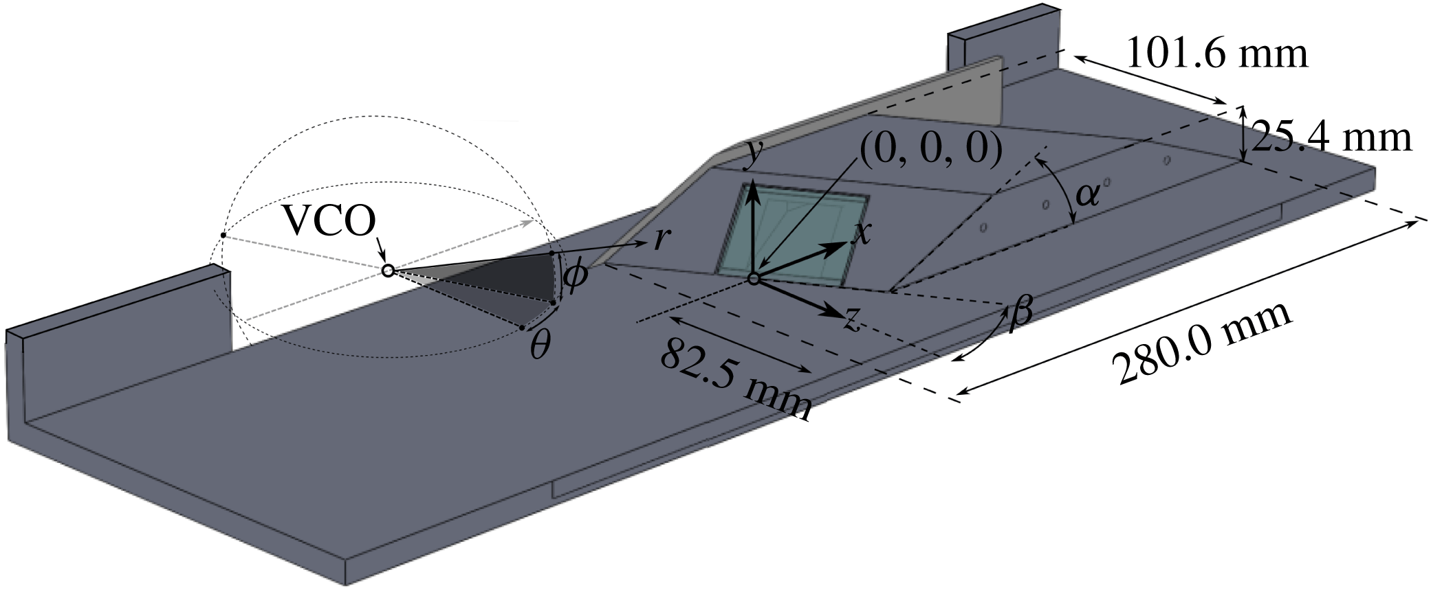
Figure 1. Tunnel cut-away with ramp and coordinate systems used in this study.
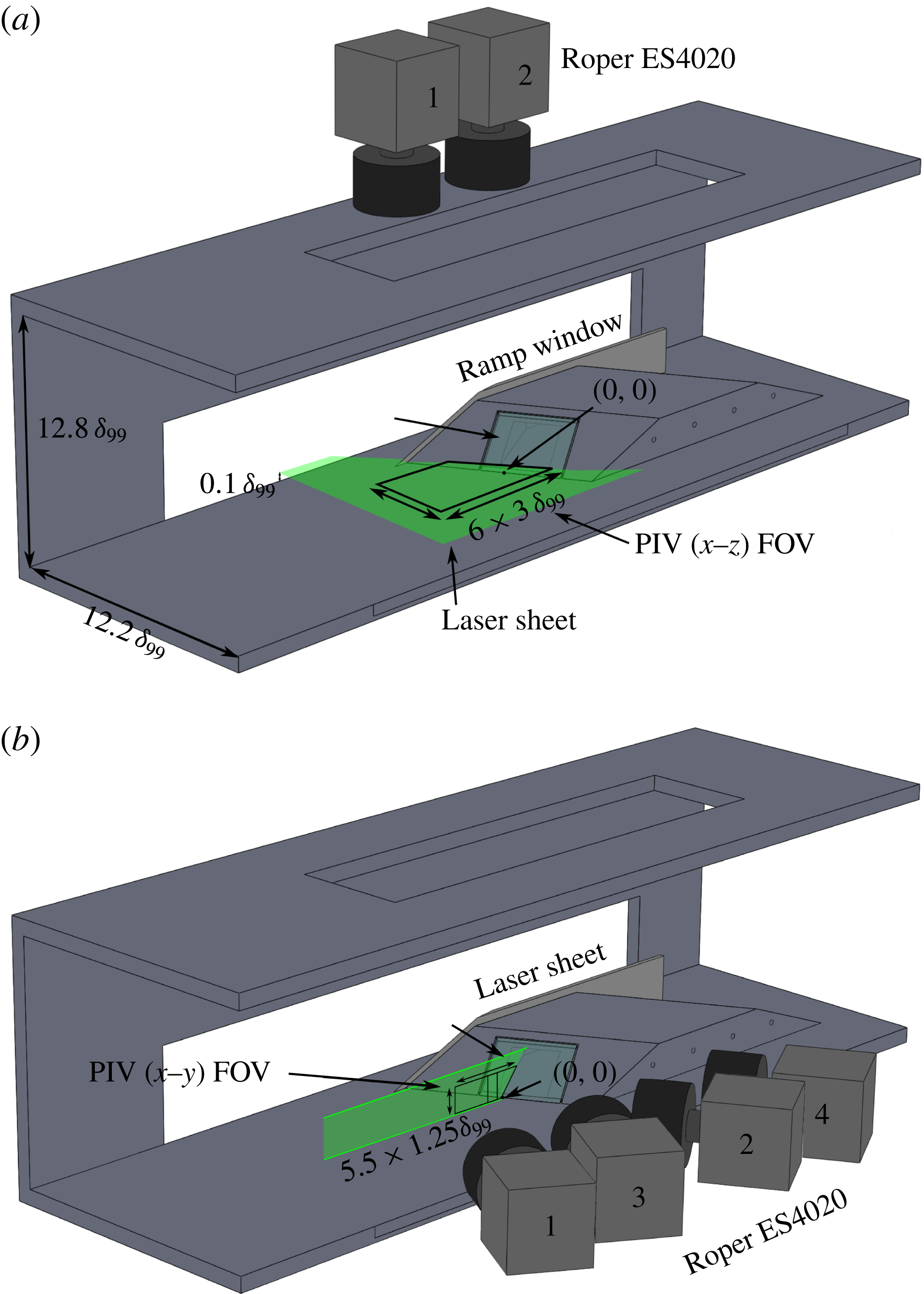
Figure 2. Tunnel cut-away with ramp and experimental set-up: (a)
 $x$
–
$x$
–
 $z$
wide-field high-resolution PIV configuration; (b)
$z$
wide-field high-resolution PIV configuration; (b)
 $x$
–
$x$
–
 $y$
stereo PIV configuration. Flow is from left to right. One of the tunnel walls is not shown.
$y$
stereo PIV configuration. Flow is from left to right. One of the tunnel walls is not shown.
2.3 Fluorescent surface flow visualization
Surface streakline visualization using an oil-flow method was used to determine the global mean structure of both interactions. In this technique, a thin mineral oil (Walmart Pharmaceuticals) was mixed with a fluorescent dye (DayGlo T13 Rocket-Red Pigment) in equal parts by volume and the floor was covered upstream of the ramp before the run starts (Vanstone et al. Reference Vanstone, Saleem, Seckin and Clemens2015). The fluorescent dye was excited using a 60 W black light and a yellow filter was used to isolate the signal from the ultraviolet light. The mixture viscosity was selected such that it was thick enough to persist for the run duration while still being thin enough that it easily moved across the tunnel floor, spreading over the entire test section on start-up. The oil flow was imaged during a run using a video camera (Basler ACA-1300-30gc 1.3 MP) that recorded at 32 frames per second and was viewed down through a ceiling window (in the position of camera 2; figure 2 a). Although the temporal response time of the surface oil flow was too slow to reflect the actual flow dynamics, visualizing the motion of the oil does aid the eye in discerning subtle flow features in the mean structure, such as regions of reattachment and reverse flow.
2.4 Wide-field high-resolution particle image velocimetry
Wide-field (5 Hz) PIV was used to examine the structure of the flow, where two (
 $x$
–
$x$
–
 $z$
plane) or four (stereo
$z$
plane) or four (stereo
 $x$
–
$x$
–
 $y$
plane) cameras were used to create a wide field of view (FOV). The stereo
$y$
plane) cameras were used to create a wide field of view (FOV). The stereo
 $x$
–
$x$
–
 $y$
plane PIV was conducted at the ramp midspan (
$y$
plane PIV was conducted at the ramp midspan (
 $z=0$
) and the
$z=0$
) and the
 $x$
–
$x$
–
 $z$
plane PIV was conducted at 10 % of the boundary-layer height. The
$z$
plane PIV was conducted at 10 % of the boundary-layer height. The
 $x$
–
$x$
–
 $z$
plane and stereo
$z$
plane and stereo
 $x$
–
$x$
–
 $y$
plane PIV experimental set-ups are shown in figures 2(a) and 2(b), respectively.
$y$
plane PIV experimental set-ups are shown in figures 2(a) and 2(b), respectively.
The PIV system consisted of a dual-cavity frequency-doubled (532 nm) Nd:YAG laser (Spectra-Physics PIV-400) and up to four frame-straddling charge-coupled device cameras (Roper ES4020) operated at a resolution of
 $2048\times 1784~\text{pixels}$
and a framing rate of 5 Hz. When conducting
$2048\times 1784~\text{pixels}$
and a framing rate of 5 Hz. When conducting
 $x$
–
$x$
–
 $z$
plane PIV (figure 2
a), two cameras were used due to restrictions in optical access through the top window. When conducting stereo
$z$
plane PIV (figure 2
a), two cameras were used due to restrictions in optical access through the top window. When conducting stereo
 $x$
–
$x$
–
 $y$
plane PIV, all four cameras could be used (figure 2
b), facilitating stereo PIV. The time separation for each PIV pulse pair was 500 ns, and the lasers delivered pulse pairs at 10 Hz. The laser sheet thickness for the
$y$
plane PIV, all four cameras could be used (figure 2
b), facilitating stereo PIV. The time separation for each PIV pulse pair was 500 ns, and the lasers delivered pulse pairs at 10 Hz. The laser sheet thickness for the
 $x$
–
$x$
–
 $z$
planar PIV was 0.5 mm and for the stereo
$z$
planar PIV was 0.5 mm and for the stereo
 $x$
–
$x$
–
 $y$
plane it was 1 mm. The stereo PIV calibration procedure involved seven calibration planes, taken between
$y$
plane it was 1 mm. The stereo PIV calibration procedure involved seven calibration planes, taken between
 $-0.75$
and 0.75 mm in steps of 0.25 centred at the middle of the laser sheet. This procedure ensured that the calibrated volume (1.5 mm thick) was larger than the laser volume (1 mm thick).
$-0.75$
and 0.75 mm in steps of 0.25 centred at the middle of the laser sheet. This procedure ensured that the calibrated volume (1.5 mm thick) was larger than the laser volume (1 mm thick).
The flow was seeded using a fluidized bed filled with titanium dioxide (
 $\text{TiO}_{2}$
) particles followed by a cyclone separator to extract the smallest particles. The nominal response time (
$\text{TiO}_{2}$
) particles followed by a cyclone separator to extract the smallest particles. The nominal response time (
 $\unicode[STIX]{x1D70F}_{p}$
) of the particles is
$\unicode[STIX]{x1D70F}_{p}$
) of the particles is
 $2.6~\unicode[STIX]{x03BC}\text{s}$
and the nominal diameter (
$2.6~\unicode[STIX]{x03BC}\text{s}$
and the nominal diameter (
 $d_{p}$
) of the particles is 260 nm; these quantities were assessed by examining the particle response through an oblique shock (Hou et al.
Reference Hou, Clemens and Dolling2003).
$d_{p}$
) of the particles is 260 nm; these quantities were assessed by examining the particle response through an oblique shock (Hou et al.
Reference Hou, Clemens and Dolling2003).
PIV data were processed using LaVision DaVis v8, which uses a multipass, adaptive interrogation scheme with an automatically adapting Gaussian-weighted subpixel interpolation. For the
 $x$
–
$x$
–
 $z$
PIV the final pass is done with a
$z$
PIV the final pass is done with a
 $32\times 32~\text{pixels}$
interrogation window and 75 % overlap. Spatial resolution is 0.02 mm per pixel and 0.64 mm per interrogation window. The accuracy of the wide-field
$32\times 32~\text{pixels}$
interrogation window and 75 % overlap. Spatial resolution is 0.02 mm per pixel and 0.64 mm per interrogation window. The accuracy of the wide-field
 $x$
–
$x$
–
 $z$
plane PIV is assessed as
$z$
plane PIV is assessed as
 $\pm 2.0~\text{m}~\text{s}^{-1}$
, based on 0.1 pixel accuracy of the particle location (Sciacchitano & Wieneke Reference Sciacchitano and Wieneke2016). The stereo
$\pm 2.0~\text{m}~\text{s}^{-1}$
, based on 0.1 pixel accuracy of the particle location (Sciacchitano & Wieneke Reference Sciacchitano and Wieneke2016). The stereo
 $x$
–
$x$
–
 $y$
plane PIV was processed in LaVision Davis v8 using adaptive Gaussian-weighted subpixel interpolation,
$y$
plane PIV was processed in LaVision Davis v8 using adaptive Gaussian-weighted subpixel interpolation,
 $32\times 32\times 4$
pixel windows and 75 % overlap. Spatial resolution is 0.02 mm per pixel and 0.63 mm per interrogation window. At this resolution it is possible to resolve down to 0.32 mm, or 2.7 % of the boundary-layer height. The accuracy of the stereo PIV is assessed as
$32\times 32\times 4$
pixel windows and 75 % overlap. Spatial resolution is 0.02 mm per pixel and 0.63 mm per interrogation window. At this resolution it is possible to resolve down to 0.32 mm, or 2.7 % of the boundary-layer height. The accuracy of the stereo PIV is assessed as
 $\pm 8.0~\text{m}~\text{s}^{-1}$
based on 0.4 pixel accuracy (Bhattacharya, Charonko & Vlachos Reference Bhattacharya, Charonko and Vlachos2017).
$\pm 8.0~\text{m}~\text{s}^{-1}$
based on 0.4 pixel accuracy (Bhattacharya, Charonko & Vlachos Reference Bhattacharya, Charonko and Vlachos2017).
Image pairs were rejected from the study if more than 5 % of the vectors were invalid or if more than 5 % of an image was more than three standard deviations from the mean. These criteria improved the quality of the averages by removing low-quality image pairs. The wide-field high-resolution
 $x$
–
$x$
–
 $z$
plane mean fields for the
$z$
plane mean fields for the
 $22.5^{\circ }$
were computed from 1268 image pairs taken from the complete set of 2069 image pairs. For the
$22.5^{\circ }$
were computed from 1268 image pairs taken from the complete set of 2069 image pairs. For the
 $19^{\circ }$
interaction, the wide-field high-resolution
$19^{\circ }$
interaction, the wide-field high-resolution
 $x$
–
$x$
–
 $z$
plane mean consists of 1364 image pairs taken from the complete dataset of 1536. The mean stereo
$z$
plane mean consists of 1364 image pairs taken from the complete dataset of 1536. The mean stereo
 $x$
–
$x$
–
 $y$
plane PIV fields were computed from 499 image pairs of the complete set of 597 image pairs. No
$y$
plane PIV fields were computed from 499 image pairs of the complete set of 597 image pairs. No
 $x$
–
$x$
–
 $y$
plane stereo PIV was taken for the
$y$
plane stereo PIV was taken for the
 $19^{\circ }$
case. The relatively high rejection rate of PIV image pairs is due to difficulty seeding consistently (i.e. ‘chugging’ of the seeder). At random times seeding density was often too high or low, even within the free stream. Assuming that the seeder chugging is uncorrelated to the boundary-layer turbulence, which is a reasonable inference, then rejecting image pairs only has the effect of diminishing the sample size and does not introduce a seeding bias.
$19^{\circ }$
case. The relatively high rejection rate of PIV image pairs is due to difficulty seeding consistently (i.e. ‘chugging’ of the seeder). At random times seeding density was often too high or low, even within the free stream. Assuming that the seeder chugging is uncorrelated to the boundary-layer turbulence, which is a reasonable inference, then rejecting image pairs only has the effect of diminishing the sample size and does not introduce a seeding bias.
3 Surface flow visualization
Sample surface flow visualization images for both the
 $19^{\circ }$
and
$19^{\circ }$
and
 $22.5^{\circ }$
interactions are shown in figures 3 and 4, respectively. The images presented are from a section of the movie where the tunnel and interaction have reached a steady state. The view is a plan view (
$22.5^{\circ }$
interactions are shown in figures 3 and 4, respectively. The images presented are from a section of the movie where the tunnel and interaction have reached a steady state. The view is a plan view (
 $x$
–
$x$
–
 $z$
plane), looking down on the interaction. The flow is from left to right and the distances have been normalized by the upstream undisturbed boundary-layer thickness (
$z$
plane), looking down on the interaction. The flow is from left to right and the distances have been normalized by the upstream undisturbed boundary-layer thickness (
 $\unicode[STIX]{x1D6FF}_{99}=11.75~\text{mm}$
). The ramp is on the right and the rectangular structure on the ramp face in figure 4 is the laser access window. Figures 3(b) and 4(b) both show a number of features superimposed onto the interaction footprint. The separation line is shown to follow the bounding sink line that the surface streaklines coalesce into. The reattachment line follows the source line that the surface streaklines are seen to diverge from. The upstream influence line marks the most upstream location at which the surface streaklines are seen to deviate from a purely streamwise direction. The separation, reattachment and upstream influence line definitions are consistent with the definitions given in Panaras (Reference Panaras1996). The intermittent region manifests as a bright region between the upstream influence and separation lines owing to the retardation and collection of fluorescent oil here. The strong cross-flow is clearly visible in the streaklines inside the interaction region.
$\unicode[STIX]{x1D6FF}_{99}=11.75~\text{mm}$
). The ramp is on the right and the rectangular structure on the ramp face in figure 4 is the laser access window. Figures 3(b) and 4(b) both show a number of features superimposed onto the interaction footprint. The separation line is shown to follow the bounding sink line that the surface streaklines coalesce into. The reattachment line follows the source line that the surface streaklines are seen to diverge from. The upstream influence line marks the most upstream location at which the surface streaklines are seen to deviate from a purely streamwise direction. The separation, reattachment and upstream influence line definitions are consistent with the definitions given in Panaras (Reference Panaras1996). The intermittent region manifests as a bright region between the upstream influence and separation lines owing to the retardation and collection of fluorescent oil here. The strong cross-flow is clearly visible in the streaklines inside the interaction region.
It is emphasized that, while the compression ramp angles chosen for this study appear close (
 $19^{\circ }$
and
$19^{\circ }$
and
 $22.5^{\circ }$
), the interactions they produce differ in size substantially, as demonstrated by the large relative changes in table 1. The sensitivity of the mean flow scale to compression angle is consistent with previous studies (Erengil & Dolling Reference Erengil and Dolling1993; Panaras Reference Panaras1996).
$22.5^{\circ }$
), the interactions they produce differ in size substantially, as demonstrated by the large relative changes in table 1. The sensitivity of the mean flow scale to compression angle is consistent with previous studies (Erengil & Dolling Reference Erengil and Dolling1993; Panaras Reference Panaras1996).

Figure 3. Fluorescent surface flow visualization for the
 $19^{\circ }$
swept compression ramp. (a) Snapshot from movie. (b) The same frame with flow details annotated. Dashed arrows are surface streaklines whose direction is extracted from the video. (c) The same frame with annotations and
$19^{\circ }$
swept compression ramp. (a) Snapshot from movie. (b) The same frame with flow details annotated. Dashed arrows are surface streaklines whose direction is extracted from the video. (c) The same frame with annotations and
 $x$
–
$x$
–
 $z$
plane PIV.
$z$
plane PIV.

Figure 4. Fluorescent surface flow visualization for the
 $22.5^{\circ }$
swept compression ramp. (a) Snapshot from movie. (b) The same frame with flow details annotated. Dashed arrows are surface streaklines whose direction is extracted from the video. (c) The same frame with annotations and
$22.5^{\circ }$
swept compression ramp. (a) Snapshot from movie. (b) The same frame with flow details annotated. Dashed arrows are surface streaklines whose direction is extracted from the video. (c) The same frame with annotations and
 $x$
–
$x$
–
 $z$
plane PIV.
$z$
plane PIV.
Table 1. Comparison of various locations in the surface flow visualization along the
 $z=0$
line for the
$z=0$
line for the
 $19^{\circ }$
and
$19^{\circ }$
and
 $22.5^{\circ }$
swept-ramp interactions shown in figures 3 and 4.
$22.5^{\circ }$
swept-ramp interactions shown in figures 3 and 4.
The surface streaklines in both figures possess a characteristic ‘S’ shape inside the separation region (highlighted in figure 4
a), which has been interpreted (for a swept interaction) in previous works as implying that a mean vortex is present (Panaras Reference Panaras1996). This ‘separation vortex’ is analogous to the recirculation region in 2D interactions, but it forms due to a combination of the recirculating flow and the cross-flow. The footprint that this separation vortex leaves on the wall is shown by the dashed arrows in figures 3 and 4. In both interactions, the surface streaklines do not exhibit true reverse flow since the streakline direction is not opposite to the free stream; instead they travel diagonally due to the significant cross-flow motion. By examining the point where the surface streaklines become tangent to the
 $z$
-direction, it is possible to extract a locus of points that represent the region with some negative streamwise (
$z$
-direction, it is possible to extract a locus of points that represent the region with some negative streamwise (
 $U$
) velocity component, as shown by the white region in figures 3(b) and 4(b). The white region in both figures is shown to fade out to represent the difficulty of extracting the exact nature of the negative
$U$
) velocity component, as shown by the white region in figures 3(b) and 4(b). The white region in both figures is shown to fade out to represent the difficulty of extracting the exact nature of the negative
 $U$
-velocity region farther downstream.
$U$
-velocity region farther downstream.
Figures 3(b) and 4(b) show that both cases also appear to be quasi-conical. Outside of the inception region, the intermittent region, separation line and reattachment line are all reasonably linear and can be traced to a single point, which has been termed the virtual conical origin (VCO) (Settles & Dolling Reference Settles and Dolling1990; Alvi & Settles Reference Alvi and Settles1992; Schmisseur & Dolling Reference Schmisseur and Dolling1994; Dolling Reference Dolling2001; Arora, Ali & Alvi Reference Arora, Ali and Alvi2015). The inception region is classically identified as the section of the SWBLI where the bulk flow features (separation, reattachment lines, etc.) are curved, which signifies that quantities within this region do not scale quasi-conically. However, as discussed later, the assumption that complete quasi-conical scaling is achieved for all quantities as soon as the bulk flow features become straight is questionable.
When the 3D swept SWBLI is considered in a spherical coordinate system with its origin at the VCO, flow quantities through the SWBLI collapse in a self-similar manner. Examining a swept 3D SWBLI in spherical coordinates is more ‘natural’ to this class of phenomenon and is used extensively in later analysis (§ 5.1).

Figure 5. Results for
 $22.5^{\circ }$
swept compression ramp. Mean stereo
$22.5^{\circ }$
swept compression ramp. Mean stereo
 $x$
–
$x$
–
 $y$
plane PIV velocity contour normalized by free-stream edge velocity. (a)
$y$
plane PIV velocity contour normalized by free-stream edge velocity. (a)
 $U$
-velocity contour. (b)
$U$
-velocity contour. (b)
 $V$
-velocity contour. (c)
$V$
-velocity contour. (c)
 $W$
-velocity contour. Chevrons mark the upstream influence, separation and reattachment locations extracted from the surface flow visualization in figure 4. Solid black line shows surrogate separation line.
$W$
-velocity contour. Chevrons mark the upstream influence, separation and reattachment locations extracted from the surface flow visualization in figure 4. Solid black line shows surrogate separation line.
4 Particle image velocimetry
The majority of PIV examined in this study was performed on the
 $22.5^{\circ }$
swept-compression-ramp case, whereas only select data are used from the
$22.5^{\circ }$
swept-compression-ramp case, whereas only select data are used from the
 $19^{\circ }$
case to enable examination of the quasi-conical nature of the flows. As shown in the surface flow visualization, the bulk flow features are similar between the two interactions.
$19^{\circ }$
case to enable examination of the quasi-conical nature of the flows. As shown in the surface flow visualization, the bulk flow features are similar between the two interactions.
4.1 Stereo
 $x$
–
$y$
:
$22.5^{\circ }$
case
$x$
–
$y$
:
$22.5^{\circ }$
case


Figure 5 shows the mean streamwise (
 $U$
), wall normal (
$U$
), wall normal (
 $V$
) and transverse (
$V$
) and transverse (
 $W$
) velocity profiles in the
$W$
) velocity profiles in the
 $x$
–
$x$
–
 $y$
plane. Figure 5(a) shows the
$y$
plane. Figure 5(a) shows the
 $U$
-velocity contours, where the blue region can be interpreted as the separation region, the turquoise to yellow region as the shear layer, and the orange to light-red region as the boundary layer fluid that is lifted over the separation region. A tiny pocket of negative velocity is observed very close to the wall (discussed further below); negative
$U$
-velocity contours, where the blue region can be interpreted as the separation region, the turquoise to yellow region as the shear layer, and the orange to light-red region as the boundary layer fluid that is lifted over the separation region. A tiny pocket of negative velocity is observed very close to the wall (discussed further below); negative
 $U$
-velocities are also observed in both surface flow visualizations. In the inflowing boundary layer, the lowest portion (yellow) interacts with the shear layer while the majority of the upper portion (red) is the section that was previously stated to flow over the interaction and exhibits relatively little interaction with it.
$U$
-velocities are also observed in both surface flow visualizations. In the inflowing boundary layer, the lowest portion (yellow) interacts with the shear layer while the majority of the upper portion (red) is the section that was previously stated to flow over the interaction and exhibits relatively little interaction with it.
Figure 5(b) shows the
 $V$
-velocity, where the red region shows the flow that has been turned upwards by the separation shock, the green region shows the inflowing boundary layer and the small green region near the ramp corner shows the separated flow. The yellow region over the separation region represents part of the shear layer and the yellow region near the separation shock line represents the smeared separation shock due to unsteadiness.
$V$
-velocity, where the red region shows the flow that has been turned upwards by the separation shock, the green region shows the inflowing boundary layer and the small green region near the ramp corner shows the separated flow. The yellow region over the separation region represents part of the shear layer and the yellow region near the separation shock line represents the smeared separation shock due to unsteadiness.
Figure 5(c) shows the
 $W$
-velocity field, the blue showing the region of strong cross-flow, which is especially strong within the surrogate separation region. The cross-flow on the ramp is clearly persistent after reattachment, a feature that is also seen in the surface flow visualization (figure 4), where the streaklines after reattachment are clearly still turning.
$W$
-velocity field, the blue showing the region of strong cross-flow, which is especially strong within the surrogate separation region. The cross-flow on the ramp is clearly persistent after reattachment, a feature that is also seen in the surface flow visualization (figure 4), where the streaklines after reattachment are clearly still turning.
It is difficult to accurately assess either true separation/shock or true separation/reattachment line locations from the average (or instantaneous) PIV given resolution limitations. Instead, surrogate values for the separation line and reattachment line are used. It is assumed that the surrogate locations are broadly representative of the true locations. The surrogate separation region is bounded by an isocontour of velocity of magnitude
 $0.2U_{\infty }$
, as shown by the solid line in figure 5(a). The surrogate separation and reattachment locations are defined by fitting a straight line to the five points on the
$0.2U_{\infty }$
, as shown by the solid line in figure 5(a). The surrogate separation and reattachment locations are defined by fitting a straight line to the five points on the
 $0.2U_{\infty }$
contour closest to the wall for each location and extrapolating to the wall, which helps to reduce noise. The distance between separation and reattachment defines the size of the separation region.
$0.2U_{\infty }$
contour closest to the wall for each location and extrapolating to the wall, which helps to reduce noise. The distance between separation and reattachment defines the size of the separation region.
A significant portion of SWBLI unsteadiness results from the movement of the separation shock foot over some region upstream of separation (the intermittent region). The most upstream location at which the inflowing boundary-layer properties are disturbed is termed the ‘upstream influence line’. When averaging, the movement of the shock foot smears the structure over the intermittent region, which makes it difficult to define in both PIV and surface flow visualization. The mean
 $x$
–
$x$
–
 $y$
plane PIV (at
$y$
plane PIV (at
 $z=0$
) shows that the upstream boundary layer mean velocity begins to be perturbed at approximately
$z=0$
) shows that the upstream boundary layer mean velocity begins to be perturbed at approximately
 $-2.62\unicode[STIX]{x1D6FF}_{99}$
, which we use as the upstream influence line. We note that the sheet is displaced from the wall and so the real upstream influence line is probably farther upstream, and different definitions of upstream influence (e.g. based on wall pressure) could give a different value. We further see that separation occurs at approximately
$-2.62\unicode[STIX]{x1D6FF}_{99}$
, which we use as the upstream influence line. We note that the sheet is displaced from the wall and so the real upstream influence line is probably farther upstream, and different definitions of upstream influence (e.g. based on wall pressure) could give a different value. We further see that separation occurs at approximately
 $-1.76\unicode[STIX]{x1D6FF}_{99}$
and reattachment near
$-1.76\unicode[STIX]{x1D6FF}_{99}$
and reattachment near
 $1.57\unicode[STIX]{x1D6FF}_{99}$
. From the surface flow visualization, we estimate that the upstream influence line is at
$1.57\unicode[STIX]{x1D6FF}_{99}$
. From the surface flow visualization, we estimate that the upstream influence line is at
 $-2.73\unicode[STIX]{x1D6FF}_{99}$
, the separation line is at
$-2.73\unicode[STIX]{x1D6FF}_{99}$
, the separation line is at
 $-1.58\unicode[STIX]{x1D6FF}_{99}$
and the reattachment is at
$-1.58\unicode[STIX]{x1D6FF}_{99}$
and the reattachment is at
 $1.32\unicode[STIX]{x1D6FF}_{99}$
. These points are shown in figure 5 by the chevrons at the wall.
$1.32\unicode[STIX]{x1D6FF}_{99}$
. These points are shown in figure 5 by the chevrons at the wall.
As discussed, figure 5(a) shows a tiny region of mean flow with negative
 $U$
-velocity right at the ramp junction, shown in white. Hence it can be seen that the swept-ramp interaction possesses a persistent region of negative
$U$
-velocity right at the ramp junction, shown in white. Hence it can be seen that the swept-ramp interaction possesses a persistent region of negative
 $U$
-velocity that extends approximately
$U$
-velocity that extends approximately
 $0.5\unicode[STIX]{x1D6FF}_{99}$
upstream of the ramp corner and is approximately
$0.5\unicode[STIX]{x1D6FF}_{99}$
upstream of the ramp corner and is approximately
 $0.025\unicode[STIX]{x1D6FF}_{99}$
in height. The very low height of this region potentially explains why it has not been observed previously. The upstream extent of the negative
$0.025\unicode[STIX]{x1D6FF}_{99}$
in height. The very low height of this region potentially explains why it has not been observed previously. The upstream extent of the negative
 $U$
-velocity region is less than suggested by the surface flow visualization, which shows upstream motion out to approximately
$U$
-velocity region is less than suggested by the surface flow visualization, which shows upstream motion out to approximately
 $-0.77\unicode[STIX]{x1D6FF}_{99}$
from the ramp corner. The reason for this disparity probably relates to PIV resolution limitations.
$-0.77\unicode[STIX]{x1D6FF}_{99}$
from the ramp corner. The reason for this disparity probably relates to PIV resolution limitations.
The presence of mean negative
 $U$
-velocity indicates that some degree of mean swirl is present within the separation region, although it is likely to be very weak (Adler & Gaitonde Reference Adler and Gaitonde2017). The stereo PIV images were examined for evidence of a mean vortex structure by examining the vorticity and the
$U$
-velocity indicates that some degree of mean swirl is present within the separation region, although it is likely to be very weak (Adler & Gaitonde Reference Adler and Gaitonde2017). The stereo PIV images were examined for evidence of a mean vortex structure by examining the vorticity and the
 $Q$
-criterion fields; however, neither of these metrics were capable of revealing coherent vortex structures, a finding reflected in Adler & Gaitonde (Reference Adler and Gaitonde2017). We attribute this result to the mean swirling motion being too weak to detect within the accuracy of the PIV. The characteristics of the
$Q$
-criterion fields; however, neither of these metrics were capable of revealing coherent vortex structures, a finding reflected in Adler & Gaitonde (Reference Adler and Gaitonde2017). We attribute this result to the mean swirling motion being too weak to detect within the accuracy of the PIV. The characteristics of the
 $W$
-velocity field appear to suggest that the cross-flow structure is more similar to a wall jet for the majority of the interaction. Further justification for this argument is presented later in § 5.3.
$W$
-velocity field appear to suggest that the cross-flow structure is more similar to a wall jet for the majority of the interaction. Further justification for this argument is presented later in § 5.3.

Figure 6. Results for
 $22.5^{\circ }$
swept compression ramp. Mean
$22.5^{\circ }$
swept compression ramp. Mean
 $x$
–
$x$
–
 $z$
plane PIV velocity contour normalized by free-stream edge velocity. (a)
$z$
plane PIV velocity contour normalized by free-stream edge velocity. (a)
 $U$
-velocity. (b)
$U$
-velocity. (b)
 $W$
-velocity. Solid black line shows surrogate separation line. Measurement plane at
$W$
-velocity. Solid black line shows surrogate separation line. Measurement plane at
 $y/\unicode[STIX]{x1D6FF}_{99}=0.1$
.
$y/\unicode[STIX]{x1D6FF}_{99}=0.1$
.

Figure 7. Results for
 $19^{\circ }$
swept compression ramp. Mean
$19^{\circ }$
swept compression ramp. Mean
 $x$
–
$x$
–
 $z$
plane PIV velocity contour normalized by free-stream edge velocity. (a)
$z$
plane PIV velocity contour normalized by free-stream edge velocity. (a)
 $U$
-velocity. (b)
$U$
-velocity. (b)
 $W$
-velocity. Solid black line shows surrogate separation line. Measurement plane at
$W$
-velocity. Solid black line shows surrogate separation line. Measurement plane at
 $y/\unicode[STIX]{x1D6FF}_{99}=0.1$
.
$y/\unicode[STIX]{x1D6FF}_{99}=0.1$
.
4.2 Wide-field planar
$x$
–
$z$
:
$22.5^{\circ }$
case


Figure 6 shows the
 $x$
–
$x$
–
 $z$
plane PIV for the
$z$
plane PIV for the
 $22.5^{\circ }$
case. In figure 6(a), the large blue region is the separation region, the turquoise represents shear-layer fluid and orange is the inflowing boundary layer. In figure 6(b) the green region is the upstream boundary layer and blue represents the region of high cross-flow. In both panels a black line is also shown that represents the surrogate separation line, which is based on the
$22.5^{\circ }$
case. In figure 6(a), the large blue region is the separation region, the turquoise represents shear-layer fluid and orange is the inflowing boundary layer. In figure 6(b) the green region is the upstream boundary layer and blue represents the region of high cross-flow. In both panels a black line is also shown that represents the surrogate separation line, which is based on the
 $0.2U_{\infty }$
isocontour. It is important to note that the plane of the
$0.2U_{\infty }$
isocontour. It is important to note that the plane of the
 $x$
–
$x$
–
 $z$
PIV is at
$z$
PIV is at
 $0.1\unicode[STIX]{x1D6FF}_{99}$
, and so the flow features inferred from surface flow visualization will be slightly different. Since the field of view for this plane does not extend over the ramp face (as the ramp blocks the laser sheet), no information is available downstream of the ramp corner and hence the reattachment location is not visible.
$0.1\unicode[STIX]{x1D6FF}_{99}$
, and so the flow features inferred from surface flow visualization will be slightly different. Since the field of view for this plane does not extend over the ramp face (as the ramp blocks the laser sheet), no information is available downstream of the ramp corner and hence the reattachment location is not visible.
Table 2. Comparison of separation line and upstream influence line locations along
 $z=0$
for both the
$z=0$
for both the
 $22.5^{\circ }$
and
$22.5^{\circ }$
and
 $19.0^{\circ }$
cases. Data for all PIV planes extracted at
$19.0^{\circ }$
cases. Data for all PIV planes extracted at
 $y/\unicode[STIX]{x1D6FF}_{99}=0.1$
.
$y/\unicode[STIX]{x1D6FF}_{99}=0.1$
.

The separation line and upstream influence locations can be extracted at
 $z=0$
for comparison with the
$z=0$
for comparison with the
 $x$
–
$x$
–
 $y$
plane PIV and surface flow visualization (SFV), as shown in table 2. Here the information for the
$y$
plane PIV and surface flow visualization (SFV), as shown in table 2. Here the information for the
 $x$
–
$x$
–
 $y$
PIV quantities are extracted at
$y$
PIV quantities are extracted at
 $y=0.1\unicode[STIX]{x1D6FF}_{99}$
to enable direct comparison. Comparison between the
$y=0.1\unicode[STIX]{x1D6FF}_{99}$
to enable direct comparison. Comparison between the
 $x$
–
$x$
–
 $y$
plane PIV (
$y$
plane PIV (
 $y=0.1\unicode[STIX]{x1D6FF}_{99}$
,
$y=0.1\unicode[STIX]{x1D6FF}_{99}$
,
 $z=0$
) and the
$z=0$
) and the
 $x$
–
$x$
–
 $z$
plane PIV (
$z$
plane PIV (
 $y=0.1\unicode[STIX]{x1D6FF}_{99}$
,
$y=0.1\unicode[STIX]{x1D6FF}_{99}$
,
 $z=0$
) is good. As the surrogate separation location is heavily influenced by the choice of isocontour value, readers are left to decide for themselves if agreement between SFV and PIV is reasonable for the
$z=0$
) is good. As the surrogate separation location is heavily influenced by the choice of isocontour value, readers are left to decide for themselves if agreement between SFV and PIV is reasonable for the
 $22.5^{\circ }$
case.
$22.5^{\circ }$
case.
4.3 Wide-field planar
$x$
–
$z$
:
$19^{\circ }$
case


Figure 7 shows the
 $x$
–
$x$
–
 $z$
plane PIV for the
$z$
plane PIV for the
 $19^{\circ }$
case; the interpretation of this figure is the same as for figure 6. Again, both figures show a surrogate separation line that has the same definition as before. While the mean structure of the
$19^{\circ }$
case; the interpretation of this figure is the same as for figure 6. Again, both figures show a surrogate separation line that has the same definition as before. While the mean structure of the
 $19^{\circ }$
case is similar to that of the
$19^{\circ }$
case is similar to that of the
 $22.5^{\circ }$
case, the interaction is much weaker, as indicated by the smaller separated flow scale. It also appears, at first viewing, that figure 7(a) shows cylindrical scaling since the upstream influence and separation lines are nearly parallel. However, examining the
$22.5^{\circ }$
case, the interaction is much weaker, as indicated by the smaller separated flow scale. It also appears, at first viewing, that figure 7(a) shows cylindrical scaling since the upstream influence and separation lines are nearly parallel. However, examining the
 $W$
-velocity (figure 7
b) clearly demonstrates that the interaction is growing and the conical nature of this interaction is obvious when examining the larger field of view provided by the surface flow visualization in figure 3. It is interesting to note, though, that an interaction that is clearly conical can be made to appear cylindrical when the field of view is limited. This point is made more relevant later (§ 5.4). The separation line and upstream influence locations can be extracted at
$W$
-velocity (figure 7
b) clearly demonstrates that the interaction is growing and the conical nature of this interaction is obvious when examining the larger field of view provided by the surface flow visualization in figure 3. It is interesting to note, though, that an interaction that is clearly conical can be made to appear cylindrical when the field of view is limited. This point is made more relevant later (§ 5.4). The separation line and upstream influence locations can be extracted at
 $z=0$
for comparison with the surface flow visualization, as shown in table 2. Again, the reader is reminded that the
$z=0$
for comparison with the surface flow visualization, as shown in table 2. Again, the reader is reminded that the
 $x$
–
$x$
–
 $z$
plane PIV is taken at a height of
$z$
plane PIV is taken at a height of
 $y=0.1\unicode[STIX]{x1D6FF}_{99}$
while the surface flow visualization is at the surface, and readers are left to make their own conclusions on agreement between PIV and surface flow visualization.
$y=0.1\unicode[STIX]{x1D6FF}_{99}$
while the surface flow visualization is at the surface, and readers are left to make their own conclusions on agreement between PIV and surface flow visualization.
5 Discussion
It was previously noted that the surface flow visualizations in figures 3 and 4 show that both interactions feature inception and quasi-conical scaling regions. Further, both the negative
 $U$
-velocity region extracted from the surface streaklines and the
$U$
-velocity region extracted from the surface streaklines and the
 $W$
-velocity component near the wall measured by PIV do not scale conically, even in the quasi-conical region. In order to better understand this region, the quasi-conical symmetry of the interaction was investigated.
$W$
-velocity component near the wall measured by PIV do not scale conically, even in the quasi-conical region. In order to better understand this region, the quasi-conical symmetry of the interaction was investigated.
5.1 Quasi-conical nature of the interaction
Figures 3 and 4 clearly demonstrate that the majority of the PIV field of view is within the region of both interactions that would normally be considered conical, as evidenced by the straight separation and reattachment lines that travel through this region. To investigate the quasi-conical scaling of the velocity fields, a spherical coordinate system is introduced with its origin at the VCO for each interaction, as shown in figures 3 and 4. This coordinate system is then overlaid onto the
 $x$
–
$x$
–
 $z$
plane PIV for the
$z$
plane PIV for the
 $19^{\circ }$
and
$19^{\circ }$
and
 $22.5^{\circ }$
cases, as shown respectively in figures 8 and 10. For comparison, the upstream influence line is shown with a dotted black line and the separation line in solid black. In this coordinate system, the velocity profiles should collapse along lines of constant radius if the flow scales quasi-conically. It is important to acknowledge that the
$22.5^{\circ }$
cases, as shown respectively in figures 8 and 10. For comparison, the upstream influence line is shown with a dotted black line and the separation line in solid black. In this coordinate system, the velocity profiles should collapse along lines of constant radius if the flow scales quasi-conically. It is important to acknowledge that the
 $x$
–
$x$
–
 $z$
plane PIV occupies the plane
$z$
plane PIV occupies the plane
 $y/\unicode[STIX]{x1D6FF}_{99}=0.1$
and as such is not a plane of constant
$y/\unicode[STIX]{x1D6FF}_{99}=0.1$
and as such is not a plane of constant
 $\unicode[STIX]{x1D719}$
. Strictly speaking, to assess quasi-conical similarity using planar PIV, the plane should sit on a plane of constant
$\unicode[STIX]{x1D719}$
. Strictly speaking, to assess quasi-conical similarity using planar PIV, the plane should sit on a plane of constant
 $\unicode[STIX]{x1D719}$
. However, it is possible to use the combination of
$\unicode[STIX]{x1D719}$
. However, it is possible to use the combination of
 $x$
–
$x$
–
 $y$
and
$y$
and
 $x$
–
$x$
–
 $z$
PIV to assess the error in assuming the
$z$
PIV to assess the error in assuming the
 $x$
–
$x$
–
 $z$
plane is at constant
$z$
plane is at constant
 $\unicode[STIX]{x1D719}$
. We assess the maximum error as being
$\unicode[STIX]{x1D719}$
. We assess the maximum error as being
 $0.07U_{\infty }$
for the
$0.07U_{\infty }$
for the
 $U$
-velocity and
$U$
-velocity and
 $0.03U_{\infty }$
for the
$0.03U_{\infty }$
for the
 $W$
-velocity. As will be shown later, this variation is not significant in relation to the variation in the velocity profiles discussed below.
$W$
-velocity. As will be shown later, this variation is not significant in relation to the variation in the velocity profiles discussed below.
Figure 9 shows velocity profiles for the
 $19^{\circ }$
swept compression ramp, along the lines of constant radius in figure 8. Similarly, figure 11 shows velocity profiles for the
$19^{\circ }$
swept compression ramp, along the lines of constant radius in figure 8. Similarly, figure 11 shows velocity profiles for the
 $22.5^{\circ }$
case along the lines of constant radius in figure 10. The velocity contours in figures 9 and 11 are shaded to match their corresponding lines in figures 8 and 10, and the upstream influence line (dotted black) and separation line (solid black) have also been added for reference.
$22.5^{\circ }$
case along the lines of constant radius in figure 10. The velocity contours in figures 9 and 11 are shaded to match their corresponding lines in figures 8 and 10, and the upstream influence line (dotted black) and separation line (solid black) have also been added for reference.

Figure 8. The
 $19^{\circ }$
swept-compression-ramp
$19^{\circ }$
swept-compression-ramp
 $x$
–
$x$
–
 $z$
plane PIV with spherical coordinate system overlaid. (a)
$z$
plane PIV with spherical coordinate system overlaid. (a)
 $U$
-velocity contour. (b)
$U$
-velocity contour. (b)
 $W$
-velocity contour. Dashed and solid black lines show the upstream influence and separation lines, respectively.
$W$
-velocity contour. Dashed and solid black lines show the upstream influence and separation lines, respectively.

Figure 9. The
 $19^{\circ }$
swept-compression-ramp normalized velocity profiles along the lines of constant radius. Profiles are shaded to correspond to the radius lines in figure 8. (a)
$19^{\circ }$
swept-compression-ramp normalized velocity profiles along the lines of constant radius. Profiles are shaded to correspond to the radius lines in figure 8. (a)
 $U$
-velocity profiles. (b)
$U$
-velocity profiles. (b)
 $W$
-velocity profiles. (c)
$W$
-velocity profiles. (c)
 $(U^{2}+W^{2})^{0.5}$
profiles. Dashed and solid black lines show upstream influence and separation lines, respectively.
$(U^{2}+W^{2})^{0.5}$
profiles. Dashed and solid black lines show upstream influence and separation lines, respectively.

Figure 10. The
 $22.5^{\circ }$
swept-compression-ramp
$22.5^{\circ }$
swept-compression-ramp
 $x$
–
$x$
–
 $z$
plane PIV with spherical coordinate system overlaid. (a)
$z$
plane PIV with spherical coordinate system overlaid. (a)
 $U$
-velocity contour. (b)
$U$
-velocity contour. (b)
 $W$
-velocity contour. Dashed and solid black lines show the upstream influence and separation lines, respectively.
$W$
-velocity contour. Dashed and solid black lines show the upstream influence and separation lines, respectively.

Figure 11. Normalized mean velocity profiles along the lines of constant radius for the
 $22.5^{\circ }$
swept compression ramp. Profiles are shaded to correspond to the radius lines in figure 10. (a)
$22.5^{\circ }$
swept compression ramp. Profiles are shaded to correspond to the radius lines in figure 10. (a)
 $U$
-velocity profiles. (b)
$U$
-velocity profiles. (b)
 $W$
-velocity profiles. (c)
$W$
-velocity profiles. (c)
 $(U^{2}+W^{2})^{0.5}$
profiles. Dashed and solid black lines show upstream influence and separation lines, respectively.
$(U^{2}+W^{2})^{0.5}$
profiles. Dashed and solid black lines show upstream influence and separation lines, respectively.
Figures 8(a) and 9(a) show that the
 $19^{\circ }$
swept-compression-ramp
$19^{\circ }$
swept-compression-ramp
 $U$
-velocity component scales quasi-conically. Similarly, figures 10(a) and 11(a) show that the
$U$
-velocity component scales quasi-conically. Similarly, figures 10(a) and 11(a) show that the
 $22.5^{\circ }$
swept-compression-ramp
$22.5^{\circ }$
swept-compression-ramp
 $U$
-velocity component also scales quasi-conically. This is demonstrated immediately from visual inspection of the alignment of velocity isocontours in figures 8(a) and 10(a) with lines of constant
$U$
-velocity component also scales quasi-conically. This is demonstrated immediately from visual inspection of the alignment of velocity isocontours in figures 8(a) and 10(a) with lines of constant
 $\unicode[STIX]{x1D703}$
. Conical scaling is also evident from inspection of the
$\unicode[STIX]{x1D703}$
. Conical scaling is also evident from inspection of the
 $U$
-velocity profiles in figures 9(a) and 11(a).
$U$
-velocity profiles in figures 9(a) and 11(a).
Examining figures 9(a) and 11(a), it can be seen that there is a small degree of spanwise variation (
 ${\sim}0.05U_{\infty }$
) in the collapse of the
${\sim}0.05U_{\infty }$
) in the collapse of the
 $U$
-velocity profiles, which is within the expected variation from examining a non-constant plane of
$U$
-velocity profiles, which is within the expected variation from examining a non-constant plane of
 $\unicode[STIX]{x1D719}$
(
$\unicode[STIX]{x1D719}$
(
 ${<}0.07U_{\infty }$
).
${<}0.07U_{\infty }$
).
The behaviour of the
 $U$
-velocity contours for both the
$U$
-velocity contours for both the
 $19^{\circ }$
and
$19^{\circ }$
and
 $22.5^{\circ }$
swept compression ramps is typical of the quasi-conical scaling detailed in the literature. In contrast, figures 9(b) and 11(b) show that the
$22.5^{\circ }$
swept compression ramps is typical of the quasi-conical scaling detailed in the literature. In contrast, figures 9(b) and 11(b) show that the
 $W$
-velocity component does not show a quasi-conical self-similarity through the SWBLI. This is also immediately obvious from inspection of figures 8(b) and 10(b), which both clearly show that the velocity isocontours align poorly with lines of constant
$W$
-velocity component does not show a quasi-conical self-similarity through the SWBLI. This is also immediately obvious from inspection of figures 8(b) and 10(b), which both clearly show that the velocity isocontours align poorly with lines of constant
 $\unicode[STIX]{x1D703}$
.
$\unicode[STIX]{x1D703}$
.
Close inspection of the
 $19^{\circ }$
and
$19^{\circ }$
and
 $22.5^{\circ }$
swept-compression-ramp profiles in figures 9(b) and 11(b) gives more information on how the
$22.5^{\circ }$
swept-compression-ramp profiles in figures 9(b) and 11(b) gives more information on how the
 $W$
-velocity scales for both cases. The inflowing boundary layer is characterized by approximately zero
$W$
-velocity scales for both cases. The inflowing boundary layer is characterized by approximately zero
 $W$
-velocity although some small variation (
$W$
-velocity although some small variation (
 ${\sim}0.01U_{\infty }$
) is observed, which is within expected error due to a non-constant
${\sim}0.01U_{\infty }$
) is observed, which is within expected error due to a non-constant
 $\unicode[STIX]{x1D719}$
(
$\unicode[STIX]{x1D719}$
(
 ${<}0.03U_{\infty }$
). As the flow enters the intermittent region, the flow is accelerated by the swept nature of the interaction and the
${<}0.03U_{\infty }$
). As the flow enters the intermittent region, the flow is accelerated by the swept nature of the interaction and the
 $W$
-velocity component increases in both cases. However, the flow clearly does not scale in a quasi-conical manner, as evidenced by the strong divergence of the
$W$
-velocity component increases in both cases. However, the flow clearly does not scale in a quasi-conical manner, as evidenced by the strong divergence of the
 $W$
-velocity profiles through the entire interaction region for both cases. This divergence is much larger than the error due to non-constant
$W$
-velocity profiles through the entire interaction region for both cases. This divergence is much larger than the error due to non-constant
 $\unicode[STIX]{x1D719}$
.
$\unicode[STIX]{x1D719}$
.
As seen in figures 9(b) and 11(b), the
 $W$
-velocity profiles closer to the VCO (darker) are accelerated to a lesser extent, resulting in a smaller cross-stream component here. Conversely, the velocity profiles farther from the VCO (lighter) are accelerated more, resulting in a stronger cross-stream component farther away from the VCO. This radial variation in the cross-stream component is also reflected in the surface flow visualizations in figures 3 and 4.
$W$
-velocity profiles closer to the VCO (darker) are accelerated to a lesser extent, resulting in a smaller cross-stream component here. Conversely, the velocity profiles farther from the VCO (lighter) are accelerated more, resulting in a stronger cross-stream component farther away from the VCO. This radial variation in the cross-stream component is also reflected in the surface flow visualizations in figures 3 and 4.
Figures 9(c) and 11(c) show the velocity magnitude (
 $(U^{2}+W^{2})^{0.5}$
) profiles for the
$(U^{2}+W^{2})^{0.5}$
) profiles for the
 $19^{\circ }$
and
$19^{\circ }$
and
 $22.5^{\circ }$
swept-compression-ramp cases, respectively. Quasi-conical scaling of the velocity magnitude is observed through the intermittent region despite the lack of quasi-conical scaling of the
$22.5^{\circ }$
swept-compression-ramp cases, respectively. Quasi-conical scaling of the velocity magnitude is observed through the intermittent region despite the lack of quasi-conical scaling of the
 $W$
-velocity through this region. Close to the separation line, the relative magnitudes of the
$W$
-velocity through this region. Close to the separation line, the relative magnitudes of the
 $U$
- and
$U$
- and
 $W$
-velocity components become comparable and hence the velocity magnitude profiles in figures 8(c) and 10(c) begin to diverge at separation. However, here the difference in the interaction strengths becomes noticeable. For the weaker
$W$
-velocity components become comparable and hence the velocity magnitude profiles in figures 8(c) and 10(c) begin to diverge at separation. However, here the difference in the interaction strengths becomes noticeable. For the weaker
 $19^{\circ }$
case, the
$19^{\circ }$
case, the
 $U$
-velocity component is not retarded to the same degree and
$U$
-velocity component is not retarded to the same degree and
 $W$
-velocities are lower and hence the
$W$
-velocities are lower and hence the
 $U$
-velocity component remains large enough that the conical scaling of the velocity magnitude is not strongly affected. For the
$U$
-velocity component remains large enough that the conical scaling of the velocity magnitude is not strongly affected. For the
 $22.5^{\circ }$
case, the
$22.5^{\circ }$
case, the
 $U$
-velocity is retarded more and the non-conical
$U$
-velocity is retarded more and the non-conical
 $W$
-velocity component is larger. Hence a stronger breakdown in conical scaling is seen in the velocity magnitudes after separation for the
$W$
-velocity component is larger. Hence a stronger breakdown in conical scaling is seen in the velocity magnitudes after separation for the
 $22.5^{\circ }$
case.
$22.5^{\circ }$
case.

Figure 12. The
 $22.5^{\circ }$
swept-compression-ramp normalized velocity profiles along the lines of constant radius. Profiles are shaded to correspond to the radius lines in figure 10. (a)
$22.5^{\circ }$
swept-compression-ramp normalized velocity profiles along the lines of constant radius. Profiles are shaded to correspond to the radius lines in figure 10. (a)
 $U_{\unicode[STIX]{x1D703}}$
-velocity profiles. (b)
$U_{\unicode[STIX]{x1D703}}$
-velocity profiles. (b)
 $U_{r}$
-velocity profiles. (c)
$U_{r}$
-velocity profiles. (c)
 $({U_{\unicode[STIX]{x1D703}}}^{2}+{U_{r}}^{2})^{0.5}$
-velocity profiles. Dashed and solid black lines show upstream influence and separation lines, respectively.
$({U_{\unicode[STIX]{x1D703}}}^{2}+{U_{r}}^{2})^{0.5}$
-velocity profiles. Dashed and solid black lines show upstream influence and separation lines, respectively.
There is, perhaps, some expectation that quasi-conical scaling should be examined in velocity components (
 $U_{r}$
,
$U_{r}$
,
 $U_{\unicode[STIX]{x1D703}}$
and
$U_{\unicode[STIX]{x1D703}}$
and
 $U_{\unicode[STIX]{x1D719}}$
) natural to the spherical coordinate system used here. However, for an interaction to be quasi-conical, any quantity must remain constant along lines of constant
$U_{\unicode[STIX]{x1D719}}$
) natural to the spherical coordinate system used here. However, for an interaction to be quasi-conical, any quantity must remain constant along lines of constant
 $\unicode[STIX]{x1D703}$
and
$\unicode[STIX]{x1D703}$
and
 $\unicode[STIX]{x1D719}$
, including velocity magnitude, which is a scalar quantity and hence independent of coordinate system. In other words, if conical scaling applies, then the velocity components
$\unicode[STIX]{x1D719}$
, including velocity magnitude, which is a scalar quantity and hence independent of coordinate system. In other words, if conical scaling applies, then the velocity components
 $U$
,
$U$
,
 $V$
and
$V$
and
 $W$
or
$W$
or
 $U_{r}$
,
$U_{r}$
,
 $U_{\unicode[STIX]{x1D703}}$
and
$U_{\unicode[STIX]{x1D703}}$
and
 $U_{\unicode[STIX]{x1D719}}$
will be constant. Indeed, figure 12 shows that conical scaling is not observed even when the velocity components are transformed into spherical coordinates. Furthermore, given that this region of the interaction does not truly scale quasi-conically, the choice of coordinate system then becomes arbitrary, as spherical coordinates are not truly natural to the flow structure. Hence, in our analysis we shall continue to examine Cartesian velocity components, as they are more intuitive.
$U_{\unicode[STIX]{x1D719}}$
will be constant. Indeed, figure 12 shows that conical scaling is not observed even when the velocity components are transformed into spherical coordinates. Furthermore, given that this region of the interaction does not truly scale quasi-conically, the choice of coordinate system then becomes arbitrary, as spherical coordinates are not truly natural to the flow structure. Hence, in our analysis we shall continue to examine Cartesian velocity components, as they are more intuitive.
The results presented suggest that the
 $U$
-velocity and velocity magnitude scale approximately quasi-conically through most of the interaction for both cases. The dominance of the
$U$
-velocity and velocity magnitude scale approximately quasi-conically through most of the interaction for both cases. The dominance of the
 $U$
-velocity seems to dictate the geometry of the interaction (separation and reattachment lines, etc.) and hence geometrical features also scale quasi-conically. However, the
$U$
-velocity seems to dictate the geometry of the interaction (separation and reattachment lines, etc.) and hence geometrical features also scale quasi-conically. However, the
 $W$
-velocity does not scale quasi-conically and begins to diverge as soon as the upstream influence line is reached and continues to do so through the interaction. Downstream of the separation line the relative contribution of the
$W$
-velocity does not scale quasi-conically and begins to diverge as soon as the upstream influence line is reached and continues to do so through the interaction. Downstream of the separation line the relative contribution of the
 $U$
-velocity becomes comparable to that of the
$U$
-velocity becomes comparable to that of the
 $W$
-velocity and quasi-conical scaling of the velocity magnitude begins to break down, although the strength of this breakdown depends upon the strength of the interaction.
$W$
-velocity and quasi-conical scaling of the velocity magnitude begins to break down, although the strength of this breakdown depends upon the strength of the interaction.
We propose that the low-magnitude velocity components in the separated flow region take much longer to reach conical similarity and as such have a much larger inception region than quantities just outside the separated flow that are dominated by fluid with momentum primarily in the
 $x$
-direction. We argue that wall pressure reaches conical similarity faster since it reflects the high-momentum fluid outside of the separated flow. Furthermore, although the velocities within the separated flow relax more slowly, it appears that they can have a significant effect on the mean separated flow structure. Indeed, it is noted by Settles et al. (Reference Settles, Perkins and Bogdonoff1980) that, even in very weakly swept SWBLI, where
$x$
-direction. We argue that wall pressure reaches conical similarity faster since it reflects the high-momentum fluid outside of the separated flow. Furthermore, although the velocities within the separated flow relax more slowly, it appears that they can have a significant effect on the mean separated flow structure. Indeed, it is noted by Settles et al. (Reference Settles, Perkins and Bogdonoff1980) that, even in very weakly swept SWBLI, where
 $W$
-velocity is especially low, the surface streaklines still turn very quickly at separation and show a marked deviation from a 2D distribution. Therefore, the slower relaxation of the velocity field inside the separated flow remains important for understanding the global flow evolution. The following discussion examines this claim in greater detail.
$W$
-velocity is especially low, the surface streaklines still turn very quickly at separation and show a marked deviation from a 2D distribution. Therefore, the slower relaxation of the velocity field inside the separated flow remains important for understanding the global flow evolution. The following discussion examines this claim in greater detail.
5.2 Normalizing quasi-conical scaling
Velocity profiles for both the
 $19^{\circ }$
and
$19^{\circ }$
and
 $22.5^{\circ }$
cases are shown in figure 13. Clearly the velocity profiles do not collapse. The
$22.5^{\circ }$
cases are shown in figure 13. Clearly the velocity profiles do not collapse. The
 $22.5^{\circ }$
case is the largest possible interaction we could facilitate within the tunnel without significant sidewall effects. There was some concern that the larger inception region in the
$22.5^{\circ }$
case is the largest possible interaction we could facilitate within the tunnel without significant sidewall effects. There was some concern that the larger inception region in the
 $W$
-velocity was a tunnel effect related to subtle sidewall contamination. The weaker
$W$
-velocity was a tunnel effect related to subtle sidewall contamination. The weaker
 $19^{\circ }$
case exhibits a separated flow that is much smaller and displays less sidewall interaction. If the profiles of these interactions can be normalized to a single profile, it implies that this effect does not relate to sidewall contamination. Baldwin et al. (Reference Baldwin, Arora, Kumar and Alvi2016) provide a method of scaling between different strength swept interactions generated by sharp fins in spherical coordinates. This normalization is given as
$19^{\circ }$
case exhibits a separated flow that is much smaller and displays less sidewall interaction. If the profiles of these interactions can be normalized to a single profile, it implies that this effect does not relate to sidewall contamination. Baldwin et al. (Reference Baldwin, Arora, Kumar and Alvi2016) provide a method of scaling between different strength swept interactions generated by sharp fins in spherical coordinates. This normalization is given as
 $$\begin{eqnarray}\unicode[STIX]{x1D703}^{\ast }=\frac{\unicode[STIX]{x1D703}-\unicode[STIX]{x1D703}_{i}}{\unicode[STIX]{x1D703}_{sweep}},\end{eqnarray}$$
where
 $\unicode[STIX]{x1D703}$
is some angle in the sharp-fin spherical coordinate system,
$\unicode[STIX]{x1D703}$
is some angle in the sharp-fin spherical coordinate system,
 $\unicode[STIX]{x1D703}_{i}$
is the inviscid shock angle and
$\unicode[STIX]{x1D703}_{i}$
is the inviscid shock angle and
 $\unicode[STIX]{x1D703}_{sweep}$
is the sweep angle, i.e. the angle between the fin wall and the separation line. Essentially this method serves to normalize the length of the arc (in spherical coordinates) that the interaction sits along. In their scaling, the interaction is referenced to some relevant feature and normalized by the sweep angle.
$\unicode[STIX]{x1D703}_{sweep}$
is the sweep angle, i.e. the angle between the fin wall and the separation line. Essentially this method serves to normalize the length of the arc (in spherical coordinates) that the interaction sits along. In their scaling, the interaction is referenced to some relevant feature and normalized by the sweep angle.


A similar normalization can be derived for the swept-ramp interactions examined here, which is given as
 $$\begin{eqnarray}\unicode[STIX]{x1D703}^{\prime }=\frac{\unicode[STIX]{x1D703}-\unicode[STIX]{x1D703}_{0}}{\unicode[STIX]{x1D703}_{sep}},\end{eqnarray}$$
where
 $\unicode[STIX]{x1D703}_{0}$
is the separation line angle and
$\unicode[STIX]{x1D703}_{0}$
is the separation line angle and
 $\unicode[STIX]{x1D703}_{sep}$
is the separation sweep angle, the angle between the straight sections of the separation and reattachment lines.
$\unicode[STIX]{x1D703}_{sep}$
is the separation sweep angle, the angle between the straight sections of the separation and reattachment lines.
The results for both the
 $19^{\circ }$
and
$19^{\circ }$
and
 $22.5^{\circ }$
cases are shown normalized by (5.2) in figure 14. Clearly the normalization given in (5.2) helps to collapse the two cases across the different interaction strengths. This is particularly true of the
$22.5^{\circ }$
cases are shown normalized by (5.2) in figure 14. Clearly the normalization given in (5.2) helps to collapse the two cases across the different interaction strengths. This is particularly true of the
 $U$
-velocity (figure 14
a), which essentially collapses down to a single distribution for both cases along any line of constant radius.
$U$
-velocity (figure 14
a), which essentially collapses down to a single distribution for both cases along any line of constant radius.
This type of normalization also helps to collapse the
 $W$
-velocity data across both cases (figure 14
b) to a single distribution that is a function of radius. The fact that the
$W$
-velocity data across both cases (figure 14
b) to a single distribution that is a function of radius. The fact that the
 $W$
-velocity profiles scale similarly, albeit not conically, suggests that the non-conical scaling seen in either case is not due to wall effects, as it would not affect each case identically. Hence, it is apparent that the
$W$
-velocity profiles scale similarly, albeit not conically, suggests that the non-conical scaling seen in either case is not due to wall effects, as it would not affect each case identically. Hence, it is apparent that the
 $W$
-velocity is still developing, proving the
$W$
-velocity is still developing, proving the
 $W$
-velocity inception region is larger than the
$W$
-velocity inception region is larger than the
 $U$
-velocity component. The next section proposes a physical interpretation of these results and presents a model of the flow field.
$U$
-velocity component. The next section proposes a physical interpretation of these results and presents a model of the flow field.
5.3 Flow field model
A conceptual illustration of the mean structure of the swept-ramp interaction is shown in figure 15. The structures highlighted within have been reconstructed from interpretation of all of the experimental data presented in this study. Features common to both interactions have been marked across both panels to avoid cluttering the figure.

Figure 15. A conceptual illustration of pertinent flow features for a SWBLI generated by a moderately swept ramp. Shaded area shows the region with a negative
 $U$
-velocity component. The panels highlight different features of the same flow field. (a) Dashed arrows show surface streaklines inside the separation region. Stations 1–4 show profiles of the separation. (b) Dashed arrows show streaklines of approaching flow, which travels over the separation and past reattachment;
$U$
-velocity component. The panels highlight different features of the same flow field. (a) Dashed arrows show surface streaklines inside the separation region. Stations 1–4 show profiles of the separation. (b) Dashed arrows show streaklines of approaching flow, which travels over the separation and past reattachment;
 $\unicode[STIX]{x1D6F9}$
shows the angle the streaklines make with the streamwise direction. Solid black arrow shows streamline of fluid inside separation region.
$\unicode[STIX]{x1D6F9}$
shows the angle the streaklines make with the streamwise direction. Solid black arrow shows streamline of fluid inside separation region.
Figure 15(a) shows the surface streaklines inside the separation region, which are derived from the surface flow visualizations in figures 3 and 4. Two lengths are shown: (i) the outboard flow inception length (
 $L_{incep1}$
), which is defined as the portion of the interaction where the separation/reattachment lines are curved and is considered not to scale conically; and (ii) the separation inception length (
$L_{incep1}$
), which is defined as the portion of the interaction where the separation/reattachment lines are curved and is considered not to scale conically; and (ii) the separation inception length (
 $L_{incep2}$
), in which the low-magnitude velocity components well within the separated flow relax to their asymptotic states. In the separation inception region, the interaction exhibits straight separation and reattachment lines, but the mean flow exhibits negative
$L_{incep2}$
), in which the low-magnitude velocity components well within the separated flow relax to their asymptotic states. In the separation inception region, the interaction exhibits straight separation and reattachment lines, but the mean flow exhibits negative
 $U$
-velocity at the wall (shaded in grey) and the cross-flow (
$U$
-velocity at the wall (shaded in grey) and the cross-flow (
 $W$
) velocity is still accelerating. For this interaction we argue that true conical similarity is achieved when the separation/reattachment lines are straight, there is no negative
$W$
) velocity is still accelerating. For this interaction we argue that true conical similarity is achieved when the separation/reattachment lines are straight, there is no negative
 $U$
-velocity present, and the
$U$
-velocity present, and the
 $W$
-velocity component is constant along radial lines. However, we expect that both the
$W$
-velocity component is constant along radial lines. However, we expect that both the
 $U$
- and
$U$
- and
 $W$
-velocities will reach the asymptotic state at different points, and that separation inception length is dependent on quantity and not a universal attribute of the SWBLI. Indeed, it is possible that other velocity statistics, such as Reynolds stresses, may take even longer to develop. It remains unknown how the criterion of negative
$W$
-velocities will reach the asymptotic state at different points, and that separation inception length is dependent on quantity and not a universal attribute of the SWBLI. Indeed, it is possible that other velocity statistics, such as Reynolds stresses, may take even longer to develop. It remains unknown how the criterion of negative
 $U$
-velocity relates to other cases.
$U$
-velocity relates to other cases.
Figure 15(b) shows notional streaklines that originate in a portion of the boundary layer that travels over the separated flow, through the free shear layer, and within the reattached boundary layer on the ramp. Upstream of the separation region these streaklines resemble those at the surface. Thus, the notional streaklines in figure 15(b) show good agreement with the surface streaklines outside of the separation region in figures 3 and 4. As the streaklines in figure 15(b) travel over the separation region they are turned, as evidenced by the swept streaklines after reattachment in figures 3 and 4. The angle (
 $\unicode[STIX]{x1D6F9}$
) made by these streaklines relative to the free stream is only constant outside the inception region, once the separation and reattachment lines are conical (straight).
$\unicode[STIX]{x1D6F9}$
) made by these streaklines relative to the free stream is only constant outside the inception region, once the separation and reattachment lines are conical (straight).
Figure 15 shows that, right at inception (station 1 in figure 15
a), the negative
 $U$
-velocity region dominates and the interaction broadly resembles a 2D interaction, with a separation line that is approximately normal to the free-stream flow and there exists only a weak cross-flow component. The separation shock becomes weaker with increasing radial ordinate owing to the sweep of the ramp. This weakening of the shock sets up a radial pressure gradient, which tends to accelerate flow in the direction of sweep. Similarly, the streamwise pressure gradient decreases with increasing radial distance, which tends to decelerate the flow less.
$U$
-velocity region dominates and the interaction broadly resembles a 2D interaction, with a separation line that is approximately normal to the free-stream flow and there exists only a weak cross-flow component. The separation shock becomes weaker with increasing radial ordinate owing to the sweep of the ramp. This weakening of the shock sets up a radial pressure gradient, which tends to accelerate flow in the direction of sweep. Similarly, the streamwise pressure gradient decreases with increasing radial distance, which tends to decelerate the flow less.
As the cross-flow component grows, the negative
 $U$
-velocity region shrinks and a transition occurs in the structure in the separation region. Near station 1 (figure 15
a) cross-flow is relatively low and negative
$U$
-velocity region shrinks and a transition occurs in the structure in the separation region. Near station 1 (figure 15
a) cross-flow is relatively low and negative
 $U$
-velocity flow is relatively large, which suggests that the mean structure is similar to a recirculating separation bubble in a 2D interaction. However, near stations 3 and 4 (figure 15
a) the cross-flow is relatively large and negative
$U$
-velocity flow is relatively large, which suggests that the mean structure is similar to a recirculating separation bubble in a 2D interaction. However, near stations 3 and 4 (figure 15
a) the cross-flow is relatively large and negative
 $U$
-velocity is relatively low, which suggests a structure more like a wall jet. This vortex/jet structure transition can be understood as a separation vortex whose radius is small (and thus strongly rotating) in the initial part of the inception region (station 1), but as the vortex grows in scale farther downstream the rotation rate slows and becomes smaller as compared to the cross-flow velocity.
$U$
-velocity is relatively low, which suggests a structure more like a wall jet. This vortex/jet structure transition can be understood as a separation vortex whose radius is small (and thus strongly rotating) in the initial part of the inception region (station 1), but as the vortex grows in scale farther downstream the rotation rate slows and becomes smaller as compared to the cross-flow velocity.
5.4 Scaling of the inception region
Conventionally, the field of view being investigated by the PIV would be viewed as being within the quasi-conical region. We present evidence that the inception region can be significantly larger for weaker quantities and it is unclear if a reasonable section of true conical flow is present for either experiment. Previous experiments on swept-ramp interactions (Settles et al. Reference Settles, Perkins and Bogdonoff1980; Erengil & Dolling Reference Erengil and Dolling1993) have been conducted at similar conditions and so it is likely that many experience similar flow structures. However, previous studies (Erengil & Dolling Reference Erengil and Dolling1993) relied more heavily on surface pressure measurements, which we argue are largely set by the outboard flow features, which achieve conical symmetry sooner. The small changes in the low-velocity separation region are unlikely to be resolvable in pressure readings and so this result was not previously detectable.
If the flow structure proposed above is correct but was simply undetectable in previous studies, then it should be possible to compare these experiments with others and make reasonable comparisons, as the driving flow structures should still be the same. Settles & Bogdonoff (Reference Settles and Bogdonoff1982) show that certain features of the inception region can be scaled using the various parameters introduced in the introduction. Particularly, Settles & Bogdonoff (Reference Settles and Bogdonoff1982), Settles & Lu (Reference Settles and Lu1985) and Settles & Dolling (Reference Settles and Dolling1990) state that the inception length can be shown to scale as
 $$\begin{eqnarray}\frac{L_{incep1}}{M_{n}}\propto \frac{\unicode[STIX]{x1D6FF}_{99}}{Re_{\unicode[STIX]{x1D6FF}_{99}}^{1/3}}.\end{eqnarray}$$
The left-hand side of (5.3) relates to parameters associated with the interaction/geometry, while the right-hand side relates to quantities related to the inflowing boundary layer. The two interactions examined in this study have the same boundary layer (nominally) and so
 $\unicode[STIX]{x1D6FF}_{99}/Re_{\unicode[STIX]{x1D6FF}_{99}}^{1/3}$
is constant (
$\unicode[STIX]{x1D6FF}_{99}/Re_{\unicode[STIX]{x1D6FF}_{99}}^{1/3}$
is constant (
 $1.63\times 10^{-4}~\text{m}$
), hence we would expect only the interaction/geometry parameters (
$1.63\times 10^{-4}~\text{m}$
), hence we would expect only the interaction/geometry parameters (
 $L_{incep1}/M_{n}$
) to vary. Table 3 shows how various quantities associated with the interaction vary between the two interactions investigated here. Settles & Bogdonoff (Reference Settles and Bogdonoff1982), Settles & Lu (Reference Settles and Lu1985) and Settles & Dolling (Reference Settles and Dolling1990) argue that the inception length (
$L_{incep1}/M_{n}$
) to vary. Table 3 shows how various quantities associated with the interaction vary between the two interactions investigated here. Settles & Bogdonoff (Reference Settles and Bogdonoff1982), Settles & Lu (Reference Settles and Lu1985) and Settles & Dolling (Reference Settles and Dolling1990) argue that the inception length (
 $L_{incep1}$
) is an important quantity in terms of scaling swept SWBLIs and we note that it appears to scale inversely with separation sweep angle (
$L_{incep1}$
) is an important quantity in terms of scaling swept SWBLIs and we note that it appears to scale inversely with separation sweep angle (
 $\unicode[STIX]{x1D703}_{sep}$
) for these experiments.
$\unicode[STIX]{x1D703}_{sep}$
) for these experiments.

Figure 16. Normalized inception length scaling as a function of separation sweep angle (
 $\unicode[STIX]{x1D703}_{sep}$
). Blue data are present study and red data are from Erengil & Dolling (Reference Erengil and Dolling1993). Crosses mark studies of quasi-conical interactions. Circles are cylindrical interactions.
$\unicode[STIX]{x1D703}_{sep}$
). Blue data are present study and red data are from Erengil & Dolling (Reference Erengil and Dolling1993). Crosses mark studies of quasi-conical interactions. Circles are cylindrical interactions.
Table 3. Comparison of various quantities related to the inception region of both the
 $19^{\circ }$
and
$19^{\circ }$
and
 $22.5^{\circ }$
cases.
$22.5^{\circ }$
cases.

Figure 16 shows how
 $L_{incep1}/\unicode[STIX]{x1D6FF}_{99}$
and
$L_{incep1}/\unicode[STIX]{x1D6FF}_{99}$
and
 $\unicode[STIX]{x1D703}_{sep}$
vary for both this experiment and those of Erengil & Dolling (Reference Erengil and Dolling1993), who performed experiments at Mach 5. Figure 16 shows two cases with nominally cylindrical scaling, which for this study were assumed to scale conically so that
$\unicode[STIX]{x1D703}_{sep}$
vary for both this experiment and those of Erengil & Dolling (Reference Erengil and Dolling1993), who performed experiments at Mach 5. Figure 16 shows two cases with nominally cylindrical scaling, which for this study were assumed to scale conically so that
 $\unicode[STIX]{x1D703}_{sep}$
could be extracted. Clearly, figure 16 demonstrates that, when inception length is normalized by boundary-layer height (
$\unicode[STIX]{x1D703}_{sep}$
could be extracted. Clearly, figure 16 demonstrates that, when inception length is normalized by boundary-layer height (
 $L_{incep1}/\unicode[STIX]{x1D6FF}_{99}$
), it decreases with increasing separation sweep angle (
$L_{incep1}/\unicode[STIX]{x1D6FF}_{99}$
), it decreases with increasing separation sweep angle (
 $\unicode[STIX]{x1D703}_{sep}$
). This shows a general agreement with the inverse relationship shown in (5.3). The inverse scaling of the inception region size with separation sweep angle is also supported by Settles & Teng (Reference Settles and Teng1984), where they note that:
$\unicode[STIX]{x1D703}_{sep}$
). This shows a general agreement with the inverse relationship shown in (5.3). The inverse scaling of the inception region size with separation sweep angle is also supported by Settles & Teng (Reference Settles and Teng1984), where they note that:
Similarly, as [
 $\unicode[STIX]{x1D703}_{sep}$
] is decreased systematically from large values, the inception length to conical flow [length] increases without bound.
$\unicode[STIX]{x1D703}_{sep}$
] is decreased systematically from large values, the inception length to conical flow [length] increases without bound.
This inverse scaling of inception length with separation sweep angle has two implications.
Firstly, interactions that are strong (large
 $\unicode[STIX]{x1D703}_{sep}$
) have a smaller inception region compared to interactions that are weak (small
$\unicode[STIX]{x1D703}_{sep}$
) have a smaller inception region compared to interactions that are weak (small
 $\unicode[STIX]{x1D703}_{sep}$
). That is, the inception region does not grow proportionately with the interaction. One possible explanation for this trend is that the radial pressure gradient associated with stronger interactions drives a stronger radial flow, which in turn erodes the inception region more effectively, resulting in smaller inception regions.
$\unicode[STIX]{x1D703}_{sep}$
). That is, the inception region does not grow proportionately with the interaction. One possible explanation for this trend is that the radial pressure gradient associated with stronger interactions drives a stronger radial flow, which in turn erodes the inception region more effectively, resulting in smaller inception regions.
The second implication is this: in the limit of very weakly diverging separation and reattachment lines (
 $\unicode[STIX]{x1D703}_{sep}\approx 0$
), the inception region is likely to be extremely long, a result that is supported by Settles & Teng (Reference Settles and Teng1984) and Lu (Reference Lu1993). Swept SWBLIs that are effectively unseparated could also be argued to have
$\unicode[STIX]{x1D703}_{sep}\approx 0$
), the inception region is likely to be extremely long, a result that is supported by Settles & Teng (Reference Settles and Teng1984) and Lu (Reference Lu1993). Swept SWBLIs that are effectively unseparated could also be argued to have
 $\unicode[STIX]{x1D703}_{sep}\approx 0$
, but unseparated interactions are not relevant to the current discussion. We speculatively suggest here, based on the reasoning above, that the only true cylindrical separated interactions are those that are unswept (
$\unicode[STIX]{x1D703}_{sep}\approx 0$
, but unseparated interactions are not relevant to the current discussion. We speculatively suggest here, based on the reasoning above, that the only true cylindrical separated interactions are those that are unswept (
 $\unicode[STIX]{x1D703}_{sep}=0$
, 2D) SWBLIs. We argue then that cylindrical scaling that has been observed in previous studies of swept separated interactions results from measurements being made in the very long inception region of weakly separated flows. In effect, the experimental domain was not large enough to observe the conical nature of the interaction. The lack of a distinction between cylindrical and conical interactions is one that is hinted at in the above quote from Settles & Teng (Reference Settles and Teng1984) and postulated by Settles & Lu (Reference Settles and Lu1985) for swept and unswept fins (although the same argument applies to swept ramps):
$\unicode[STIX]{x1D703}_{sep}=0$
, 2D) SWBLIs. We argue then that cylindrical scaling that has been observed in previous studies of swept separated interactions results from measurements being made in the very long inception region of weakly separated flows. In effect, the experimental domain was not large enough to observe the conical nature of the interaction. The lack of a distinction between cylindrical and conical interactions is one that is hinted at in the above quote from Settles & Teng (Reference Settles and Teng1984) and postulated by Settles & Lu (Reference Settles and Lu1985) for swept and unswept fins (although the same argument applies to swept ramps):
The literature does not clarify whether the interaction is asymptotically cylindrical or conical in nature. Since sharp unbounded bodies naturally produce conical fields in supersonic flow, it appears likely to the present authors that earlier observations of quasi-cylindrical fin interactions were unintentionally contaminated by limited test channel or generator dimensions.
Wang & Bogdonoff (Reference Wang and Bogdonoff1986) also note a difficulty in discerning between the conical and cylindrical regimes and note a difficulty in applying either concept over large regions:
The present analysis shows that the previous conical/cylindrical designation and boundaries are only approximations, and that the conical proposal is only locally applicable.
This lack of a real distinction between conical and cylindrical interactions is supported by figure 16. This figure contains two results from ‘cylindrical’ interactions (circles) which can be seen to fall onto the same distribution as the quasi-conical results (crosses) – suggesting they are part of the same regime. The reason for mistaking slow-growing quasi-conical interactions as cylindrical relates to the scale of the experiment versus the SWBLI and is illustrated in figure 17. Figure 17 shows a weakly growing quasi-conical ramp interaction (
 $\unicode[STIX]{x1D703}_{sep}\approx 0$
);
$\unicode[STIX]{x1D703}_{sep}\approx 0$
);
 $L_{Sep1}$
,
$L_{Sep1}$
,
 $L_{Sep2}$
and
$L_{Sep2}$
and
 $L_{Sep3}$
are all different lengths and the separation inception region (
$L_{Sep3}$
are all different lengths and the separation inception region (
 $L_{incep2}$
) is much larger than for the outboard flow (
$L_{incep2}$
) is much larger than for the outboard flow (
 $L_{incep1}$
), as suggested above.
$L_{incep1}$
), as suggested above.
As previously stated, this study asserts that the only ‘true’ separated cylindrical interaction is a 2D SWBLI. As discussed, at inception the interaction strongly resembles a 2D interaction. Dominant quantities, such as
 $U$
-velocity, have relatively high gradients and the departure from this relatively 2D state near inception to the quasi-conical state is clear, and has traditionally been observed to coincide with strong curvature of the surface flow features (separation, reattachment, etc.). However, weaker quantities, such a
$U$
-velocity, have relatively high gradients and the departure from this relatively 2D state near inception to the quasi-conical state is clear, and has traditionally been observed to coincide with strong curvature of the surface flow features (separation, reattachment, etc.). However, weaker quantities, such a
 $W$
-velocity, vary much more slowly and so require a much larger field of view before reaching quasi-conical symmetry. If the field of view of the experiment is limited such that the
$W$
-velocity, vary much more slowly and so require a much larger field of view before reaching quasi-conical symmetry. If the field of view of the experiment is limited such that the
 $U$
-velocity inception length is small but weaker quantities (such as
$U$
-velocity inception length is small but weaker quantities (such as
 $W$
-velocity) are still slowly changing away from the 2D conditions near the inception point, then it may well be that the interaction would appear to have a 2D, cylindrical appearance.
$W$
-velocity) are still slowly changing away from the 2D conditions near the inception point, then it may well be that the interaction would appear to have a 2D, cylindrical appearance.
This situation is shown by the dotted box in figure 17. When the SWBLI in figure 17 is only examined within this experimental field of view, then the interaction appears cylindrical as
 $L_{Sep1}$
and
$L_{Sep1}$
and
 $L_{Sep2}$
are very similar. A similar result was observed when examining the current experiments – when viewing the
$L_{Sep2}$
are very similar. A similar result was observed when examining the current experiments – when viewing the
 $19^{\circ }$
case, the
$19^{\circ }$
case, the
 $U$
-velocity fields indicated cylindrical scaling, but when viewing the wider field of view provided by the surface flow visualization (figure 3), the conical nature of the interaction was apparent.
$U$
-velocity fields indicated cylindrical scaling, but when viewing the wider field of view provided by the surface flow visualization (figure 3), the conical nature of the interaction was apparent.

Figure 17. Diagram showing a weakly growing quasi-conical interaction (
 $\unicode[STIX]{x1D703}_{sep}\approx 0$
). (b) A section of the interaction is highlighted and expanded to show how, when the field of view is restricted relative to the growth of the SWBLI, it can appear cylindrical.
$\unicode[STIX]{x1D703}_{sep}\approx 0$
). (b) A section of the interaction is highlighted and expanded to show how, when the field of view is restricted relative to the growth of the SWBLI, it can appear cylindrical.
Although our view and that of Settles & Teng (Reference Settles and Teng1984) regarding the nature of conical versus cylindrical scaling differ substantially, it is interesting that some of the observations made in this study agree with the implications of the Settles & Teng (Reference Settles and Teng1984) model. For example, their model leads to an inverse scaling relationship between interaction size (
 $\unicode[STIX]{x1D703}_{sep}$
) and the inception length. Both interactions examined in our study, which would be attached in an inviscid flow, would be considered detached by Settles & Teng (Reference Settles and Teng1984) (owing to the use of a Mach number that differs from the free-stream value), and therefore they would argue that this would make them conical – which they are. In other words, Settles & Teng (Reference Settles and Teng1984) do not evaluate the shock attachment using the free-stream Mach number. Instead, they use the slip Mach number: the Mach number at the top of the inner deck (from triple deck theory), which is then resolved normal to the ramp edge for 2D comparison. The slip Mach number is substantially less than that of the free stream; hence, Settles & Teng (Reference Settles and Teng1984) inherently limit cylindrical interactions to relatively weak interactions for any given conditions, by evaluating shock detachment at a much lower Mach number than the free stream. This model becomes a shock strength argument of sorts, and while their rationale is different than ours, it essentially leads to similar observations regarding cylindrical versus conical scaling. We argue that cylindrical scaling is observed for weak interactions because the inception region is exceptionally long and thus the asymptotic state is not achieved in typical university wind tunnels. In their view the interactions are genuinely cylindrical and presumably remain so infinitely far downstream. While we are not able to prove or disprove either model, they do lead to different behaviours at large radial distances, which provides an important validation test that future researchers could pursue.
$\unicode[STIX]{x1D703}_{sep}$
) and the inception length. Both interactions examined in our study, which would be attached in an inviscid flow, would be considered detached by Settles & Teng (Reference Settles and Teng1984) (owing to the use of a Mach number that differs from the free-stream value), and therefore they would argue that this would make them conical – which they are. In other words, Settles & Teng (Reference Settles and Teng1984) do not evaluate the shock attachment using the free-stream Mach number. Instead, they use the slip Mach number: the Mach number at the top of the inner deck (from triple deck theory), which is then resolved normal to the ramp edge for 2D comparison. The slip Mach number is substantially less than that of the free stream; hence, Settles & Teng (Reference Settles and Teng1984) inherently limit cylindrical interactions to relatively weak interactions for any given conditions, by evaluating shock detachment at a much lower Mach number than the free stream. This model becomes a shock strength argument of sorts, and while their rationale is different than ours, it essentially leads to similar observations regarding cylindrical versus conical scaling. We argue that cylindrical scaling is observed for weak interactions because the inception region is exceptionally long and thus the asymptotic state is not achieved in typical university wind tunnels. In their view the interactions are genuinely cylindrical and presumably remain so infinitely far downstream. While we are not able to prove or disprove either model, they do lead to different behaviours at large radial distances, which provides an important validation test that future researchers could pursue.
5.5 Local similarity of the extended inception region
While the
 $W$
-velocity components do not scale quasi-conically, an analogous form of self-similarity was observed. At this point it is convenient to introduce a new
$W$
-velocity components do not scale quasi-conically, an analogous form of self-similarity was observed. At this point it is convenient to introduce a new
 $W$
-velocity contour line which is very similar in concept to the
$W$
-velocity contour line which is very similar in concept to the
 $U$
-velocity surrogate separation line. This line is defined as the contour line of
$U$
-velocity surrogate separation line. This line is defined as the contour line of
 $-0.08W/U_{\infty }$
and is termed the ‘surrogate cross-flow line’. The value for this contour was chosen somewhat arbitrarily as the
$-0.08W/U_{\infty }$
and is termed the ‘surrogate cross-flow line’. The value for this contour was chosen somewhat arbitrarily as the
 $W$
-velocity at the separation location at
$W$
-velocity at the separation location at
 $z=0$
. Much like the quasi-conical section, the choice of features is unimportant as long as it follows the growth of the
$z=0$
. Much like the quasi-conical section, the choice of features is unimportant as long as it follows the growth of the
 $W$
-velocity, which isocontours do. The surrogate cross-flow lines are shown for both cases in figure 18 and clearly do not grow conically. The surrogate cross-flow line is analogous to the separation line and will be termed the ‘cross-flow separation angle’ (
$W$
-velocity, which isocontours do. The surrogate cross-flow lines are shown for both cases in figure 18 and clearly do not grow conically. The surrogate cross-flow line is analogous to the separation line and will be termed the ‘cross-flow separation angle’ (
 $\unicode[STIX]{x1D703}_{W}$
) when considered in spherical coordinates. Owing to the nonlinear growth of the
$\unicode[STIX]{x1D703}_{W}$
) when considered in spherical coordinates. Owing to the nonlinear growth of the
 $W$
-velocity profiles, the cross-flow separation angle is a function of radius when considered in relation to the spherical coordinate systems used to scale both of the cases conically. The cross-flow separation angle can be substituted for the separation angle in (5.2) and used to scale the
$W$
-velocity profiles, the cross-flow separation angle is a function of radius when considered in relation to the spherical coordinate systems used to scale both of the cases conically. The cross-flow separation angle can be substituted for the separation angle in (5.2) and used to scale the
 $W$
-velocity component, giving the new scaling quantity
$W$
-velocity component, giving the new scaling quantity
 $$\begin{eqnarray}\unicode[STIX]{x1D703}^{\prime \prime }=\frac{\unicode[STIX]{x1D703}-\unicode[STIX]{x1D703}_{W}}{\unicode[STIX]{x1D703}_{sep}}.\end{eqnarray}$$
Figure 19 shows normalized
 $W$
-velocity profiles along lines of constant radius for both the
$W$
-velocity profiles along lines of constant radius for both the
 $19^{\circ }$
and
$19^{\circ }$
and
 $22.5^{\circ }$
cases. Figures 19(a) to 19(c) show the
$22.5^{\circ }$
cases. Figures 19(a) to 19(c) show the
 $W$
-velocity contours which were normalized for quasi-conical scaling. Figures 19(d) and 19(e) have been normalized using the scaling in (5.4). As can be seen, the
$W$
-velocity contours which were normalized for quasi-conical scaling. Figures 19(d) and 19(e) have been normalized using the scaling in (5.4). As can be seen, the
 $W$
-velocity profiles collapse well, not only for each case (figure 19
d,e) but also between cases (figure 19
f). Hence, it is apparent that even the inception region of a SWBLI scales in some sort of self-similar manner.
$W$
-velocity profiles collapse well, not only for each case (figure 19
d,e) but also between cases (figure 19
f). Hence, it is apparent that even the inception region of a SWBLI scales in some sort of self-similar manner.

Figure 18. Average
 $x$
–
$x$
–
 $z$
plane PIV
$z$
plane PIV
 $W$
-velocity contours for the
$W$
-velocity contours for the
 $19^{\circ }$
(a) and
$19^{\circ }$
(a) and
 $22.5^{\circ }$
(b) cases normalized by free-stream edge velocity. Black line shows the surrogate cross-flow line.
$22.5^{\circ }$
(b) cases normalized by free-stream edge velocity. Black line shows the surrogate cross-flow line.


6 Conclusion
This study combines information from PIV captured in two different planes (i.e.
 $x$
–
$x$
–
 $y$
and
$y$
and
 $x$
–
$x$
–
 $z$
) and surface flow visualization to infer information about the mean flow structure of two SWBLIs generated by swept ramps with the same compression angle but different sweep angles. For the swept interactions examined in this study, it is shown that, outside of the expected inception region, the lines of upstream influence, separation and reattachment derived from the surface flow visualization all exhibit conical scaling, as do the
$z$
) and surface flow visualization to infer information about the mean flow structure of two SWBLIs generated by swept ramps with the same compression angle but different sweep angles. For the swept interactions examined in this study, it is shown that, outside of the expected inception region, the lines of upstream influence, separation and reattachment derived from the surface flow visualization all exhibit conical scaling, as do the
 $U$
-velocity and
$U$
-velocity and
 $U_{\unicode[STIX]{x1D703}}$
-velocity profiles. However, the
$U_{\unicode[STIX]{x1D703}}$
-velocity profiles. However, the
 $W$
-velocity profiles take considerably longer to reach their asymptotic state, and do not scale conically over the fields of view considered. Essentially, the bulk flow features develop quasi-conically, but the velocity field within the separated flow does not.
$W$
-velocity profiles take considerably longer to reach their asymptotic state, and do not scale conically over the fields of view considered. Essentially, the bulk flow features develop quasi-conically, but the velocity field within the separated flow does not.
We interpret these results as meaning that the separated flow region is considerably more sensitive to how the flow originates and therefore takes longer to relax to the quasi-conical state and implies that inception length is quantity-specific and not a global feature of any given SWBLI. The relative sizes of the different inception regions seem to be related to the global strength of the interaction. It is shown that stronger interactions have shorter inception lengths, while weaker interactions have longer ones. Examining the limit of this relationship provides further insight into the possible nature of cylindrical interactions, which we argue are not truly cylindrical but are actually weak quasi-conical cases, although this result requires further study to justify fully. Finally, two scaling laws (
 $\unicode[STIX]{x1D703}^{\prime }$
and
$\unicode[STIX]{x1D703}^{\prime }$
and
 $\unicode[STIX]{x1D703}^{\prime \prime }$
) are developed that collapse both
$\unicode[STIX]{x1D703}^{\prime \prime }$
) are developed that collapse both
 $U$
- and
$U$
- and
 $W$
-velocity profiles and are in agreement with the literature. These scaling laws demonstrate that, while the inception region does not scale quasi-conically, it still grows self-similarly for the region examined.
$W$
-velocity profiles and are in agreement with the literature. These scaling laws demonstrate that, while the inception region does not scale quasi-conically, it still grows self-similarly for the region examined.
Acknowledgements
This work is sponsored by the AFOSR under grant FA9550-14-1-0167 with I. Leyva as the programme manager. This source of support is gratefully acknowledged.


