


1. Introduction
Particle dynamics in a turbulent flow are an important consideration in several applications, which range from small-scale phenomena like transport of blood corpuscles in the human body (Dooley & Quinlan Reference Dooley and Quinlan2009) to large-scale astrophysical flows (Bracco et al. Reference Bracco, Chavanis, Provenzale and Spiegel1999). Sediment transport in rivers and oceans, pollutant transport in the atmosphere, volcanic ash eruptions and fluidised bed reactors are some of the more commonplace applications. The dynamics associated with particle interactions in a turbulent flow becomes richer when the particles are fluid too, as in air bubbles in a turbulent liquid flow (Balachandar & Eaton Reference Balachandar and Eaton2010) or liquid droplets in a turbulent air flow (Grabowski & Wang Reference Grabowski and Wang2013). The latter scenario, which is of great interest in propulsion systems (Reveillon & Vervisch Reference Reveillon and Vervisch2005) and warm rain initiation (Wilkinson, Mehlig & Bezuglyy Reference Wilkinson, Mehlig and Bezuglyy2006), is the topic of the current study. Specifically, we investigate droplet size growth arising from coalescence in a background turbulent air flow, a mechanism thought to be of significance in warm rain formation (Falkovich, Fouxon & Stepanov Reference Falkovich, Fouxon and Stepanov2002).
Droplet size growth arising from air turbulence depends directly on droplet collision rates, although collisions do not necessarily result in coalescence. An estimation of droplet collision rates therefore represents an important first step towards an understanding of trends in the evolution of droplet size in turbulent flows. The parameters that influence droplet collision rates include both turbulent flow features, such as its length scales and intensity (Vaillancourt & Yau Reference Vaillancourt and Yau2000), and droplet features, such as its size distribution, volume fraction and the liquid density (Freud & Rosenfeld Reference Freud and Rosenfeld2012). Owing to the strong coupling between these various parameters, accounting for all of their effects simultaneously on droplet collision rates is challenging. For similar-sized droplets, whose size is much smaller than the Kolmogorov length scale of the turbulent flow, their collision rates depend primarily on the droplet size, the droplet number density, the turbulence dissipation rate and the air kinematic viscosity (Saffman & Turner Reference Saffman and Turner1956). For particles much larger than the Kolmogorov length scale, Abrahamson (Reference Abrahamson1975) used kinetic theory to estimate their collision rates. The collision rates in intermediate particles, however, are poorly captured by both the small- and large-droplet theories. By performing direct numerical simulations for intermediate-sized particles in the dilute limit, Sundaram & Collins (Reference Sundaram and Collins1997) highlighted two important effects, namely preferential concentration (i.e. spatial inhomogeneity in local number density) and particle decorrelation (increased relative velocity between droplets), which enhance collision rates. Several studies have since focused on various mechanisms that affect the preferential concentration and particle decorrelation effects.
In regards to preferential concentration, two primary mechanisms have been discussed in the literature. Particles whose density is much larger than air density and of Stokes number  $St \sim 1$ tend to get centrifuged out of turbulent eddies and accumulate in low-vorticity regions (Maxey Reference Maxey1987; Squires & Eaton Reference Squires and Eaton1991; Eaton & Fessler Reference Eaton and Fessler1994; Jacobs et al. Reference Jacobs, Merchant, Jendrassak, Limpasuvan, Gurka and Hackett2016). This clustering can in turn locally increase the droplet number density, and hence increase the droplet collision rates in turbulent flows with a small mean flow (Sundaram & Collins Reference Sundaram and Collins1997). The centrifugal mechanism, however, is relatively less effective at
  $St$ far from unity. In contrast to clustering arising from a centrifugal mechanism, where the small scales significantly influence clustering, large inertial particles usually undergo multi-scale clustering (Coleman & Vassilicos Reference Coleman and Vassilicos2009). The physical mechanism attributed to a preferential concentration for
  $St >1$ is the sweep-stick mechanism (Goto & Vassilicos Reference Goto and Vassilicos2008). In the sweep-stick mechanism, inertial particles have been shown to accumulate in zero-acceleration regions, with the resulting cluster convecting with the carrier fluid (Goto & Vassilicos Reference Goto and Vassilicos2008; Monchaux, Bourgoin & Cartellier Reference Monchaux, Bourgoin and Cartellier2012). The effect of this sweep-stick clustering mechanism on droplet collision rates is not well understood. Furthermore, large-scale flow anisotropy can also enhance particle collisions by introducing anisotropy in the geometric configurations of small-scale clustering even if the turbulence is isotropic at small scales (Gualtieri et al. Reference Gualtieri, Picano, Sardina and Casciola2012).
In regards to particle decorrelation, various mechanisms, namely caustics (Wilkinson et al. Reference Wilkinson, Mehlig and Bezuglyy2006), sling effect (Falkovich et al. Reference Falkovich, Fouxon and Stepanov2002) and differential settling velocity (Good et al. Reference Good, Ireland, Bewley, Bodenschatz, Collins and Warhaft2014; Jacobs et al. Reference Jacobs, Merchant, Jendrassak, Limpasuvan, Gurka and Hackett2016), have been discussed. Caustics (Bec et al. Reference Bec, Biferale, Cencini, Lanotte and Toschi2010) and the sling effect (Voßkuhle et al. Reference Voßkuhle, Pumir, Lévêque and Wilkinson2014) both lead to enhanced droplet collisions beyond a threshold turbulence intensity by inducing a very high relative velocity even at small separation distances. While the underlying mechanism in caustics is the multi-valued velocity field in phase space (Wilkinson et al. Reference Wilkinson, Mehlig and Bezuglyy2006), the sling effect concerns particles being ‘slung’ by vortices (Falkovich & Pumir Reference Falkovich and Pumir2007). However, droplet collisions induced by differential settling, which results from particle inertia, are relatively weak (Voßkuhle et al. Reference Voßkuhle, Pumir, Lévêque and Wilkinson2014).
While several studies have focused on monodisperse droplet fields, real-world droplet fields, such as clouds, are polydisperse, i.e. they comprise a finite range of droplet sizes. Indeed, droplet collisions followed by coalescence may itself be responsible for introducing polydispersity in a monodisperse droplet field. The dynamics across different droplet sizes in a polydisperse droplet field may introduce non-trivial effects that are absent in monodisperse droplets. For polydisperse droplet fields, studies on droplet collisions have focused either on preferential concentration (Reade & Collins Reference Reade and Collins2000; Aliseda et al. Reference Aliseda, Cartellier, Hainaux and Lasheras2002) or particle decorrelation (James & Ray Reference James and Ray2017). Preferential concentration and particle decorrelation are, however, physically coupled (Bec et al. Reference Bec, Celani, Cencini and Musacchio2005). A recent experimental study (Kumar, Chakravarthy & Mathur Reference Kumar, Chakravarthy and Mathur2019) showed that for a given polydisperse droplet field in which preferential concentration and particle decorrelation simultaneously occur in a turbulent air flow with a strong mean component, there exists an optimum turbulence intensity for which droplet size growth is maximised. They report that the onset of clustering suppresses the intuitive effect of an increase in droplet collision rate with air turbulence intensity, which results in the existence of an optimum air turbulence intensity that maximises the average droplet size growth rate arising from droplet coalescence. The study by Kumar et al. (Reference Kumar, Chakravarthy and Mathur2019) was restricted to a fixed initial droplet field, and hence did not investigate the effects of the initial droplet characteristics.
In this paper, we report on the effects of mean droplet size and number density on the droplet size growth rate in a strongly polydisperse droplet field in a background turbulent air flow. The rest of the paper is organised as follows. Section 2 describes the set-up, which includes the various measurement techniques used in this study, and lists the various experimental parameters and their values. The experimental results, along with a detailed interpretation using various post-processing tools, are presented in § 3. Our results are summarised in § 4, followed by a brief discussion of the relevance of our results to warm rain initiation.
2. Methodology
The experimental set-up consisted of a vertically oriented air flow facility, at the top of which air flow at a desired mass flow rate entered through an inlet manifold. The air flow then passed through honeycomb structures (having holes with a diameter of 5 mm) and a converging duct of a square cross-section, as shown in figure 1(a). Within the constant area duct placed downstream of the converging duct, an ATG (Mulla, Sampath & Chakravarthy Reference Mulla, Sampath and Chakravarthy2019) was placed that imparted turbulence on the incoming flow. Polydisperse water droplets with diameters in the range of 0–120  $\mathrm {\mu }$m were introduced into the turbulent air flow through a spray nozzle placed at the air flow exit (figure 1a). We defined a
  $xy$ coordinate system such that
  $x$ is the axial distance from the spray nozzle exit and
  $y$ is the transverse coordinate measured from the central axis.

Figure 1. (a) Schematic of the experimental set-up, with all dimensions in mm. The axial and transverse directions are specified by the  $x$- and
  $y$-axes, respectively, with the origin placed at the spray nozzle exit. (b) Top view of the AA
 $^\prime$ plane indicated in (a), along with the optical arrangements for the phase Doppler interferometry (PDI) and long-distance microscopy (LDM) measurements. (c) Schematic representation of the active turbulence generator (ATG), with 8 horizontal and 8 vertical rods arranged in a
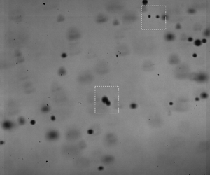
  $270\ \textrm {mm}\times 270\ \textrm {mm}$ square region. (d) A representative image obtained using LDM over a
  $4.5\ \textrm {mm}\times 4.5\ \textrm {mm}$ window centred around
  $(x,y) = (302.25,0)$ mm.
The ATG comprised a series of rotating vanes arranged on a  $270\ \textrm {mm} \times 270\ \textrm {mm}$ square cross-section, driven by 24 independently controlled stepper motors. A schematic of the ATG is shown in figure 1(c). A grid spacing (
 $M$) of 32.5 mm was used to fit eight horizontal and vertical shafts arranged in the
  $270\ \textrm {mm} \times 270\ \textrm {mm}$ (
 $8M \times 8M$) square box (figure 1c). To reduce inertia, instead of rods, tubes with an inner diameter of 6 mm and a wall thickness of 1 mm were used. The horizontal shafts and vertical shafts were placed at different planes which were separated by 11 mm. Aluminium vanes, with a chord length of 31.6 mm and thickness of 0.5 mm, were mounted on the tube alternatively on each side of the rod. Each rod was connected to a stepper motor through deep groove ball bearings. The angular velocity was modelled as a random variable and the rotation profile of the vanes controlled the turbulence intensity imparted to the air flow. Another converging duct, placed downstream of the ATG, improved the isotropy of turbulence before the air flow exited into the open surroundings.
Two different measurement techniques were employed to characterize the droplet field in a region that was sufficiently far from the spray nozzle exit. Phase Doppler interferometry (Bachalo Reference Bachalo1997) was used to measure the distributions of droplet diameter and velocity at different axial and transverse locations. In addition, the PDI data were also used to estimate the droplet number density, following the algorithm described in Qiu & Sommerfeld (Reference Qiu and Sommerfeld1992) and Borée, Ishima & Flour (Reference Borée, Ishima and Flour2001). Long-distance microscopy was used to visualize individual droplet events and subsequently compute statistical measures of these events. The  $\it {Artium}$-made PDI set-up consists of a 500 mm focal length transmitter and receiver, which measures droplet sizes in the range of 0.3–8000
  $\mathrm {\mu }$m with an accuracy of
  $\pm$0.5
  $\mathrm {\mu }$m. The LDM set-up consisted of a strobe light source that was placed approximately 1 m from the central axis, and a high-speed camera (FASTCAM series from Photron with a maximum resolution of
  $1024\times 1024$ at 5400 Hz and a minimum of
  $128\times 16$ at 500 000 Hz) fitted with a microscope (QM-100 model from Questar with manual focusing) that captured images at 10 000 Hz with
  $768\ \textrm {pixels}\times 768\ \textrm {pixels}$ on the camera representing the
  $4.5\ \textrm {mm}\times 4.5\ \textrm {mm}$ field of view with a 3.5 mm depth of field. Figure 1(b) shows the optical arrangements for both PDI and LDM. A sample LDM image is shown in figure 1(d), which typically captured a couple of tens of droplets in a single frame. The frame resolution was such that a 60
  $\mathrm {\mu }$m droplet occupied approximately 10 pixels in each direction. We also performed three-dimensional laser Doppler velocimetry (LDV) measurements without the spray, with olive oil droplets of 1
  $\mathrm {\mu }$m acting as seeding particles, to quantify the turbulent intensity at various experimental settings.
The PDI, LDM and LDV measurements were performed in a region that was sufficiently downstream of the spray nozzle such that transverse variations of droplet characteristics were negligible, and thus indicated a good mixing of the droplet field and the background turbulent air flow. Accordingly, the measurement region was identified as the rectangular domain specified by  $-20\le y\le 20$ and
  $200\le x\le 400$ mm. Experimental measurements showing transverse uniformity in this region have been reported by Kumar et al. (Reference Kumar, Chakravarthy and Mathur2019). Specifically, PDI and LDV measurements were performed at various transverse and axial locations within the measurement region, while LDM was focused on a smaller subset region given by
  $-2.25\le y\le 2.25$ and
  $300 \le x\le 304.5$ mm (see figure 1d). Various flow and droplet characteristics were estimated from the LDV and PDI measurements, based on the expressions given in Appendix A.
For a given spray nozzle operating at a fixed injection pressure, experiments were run at different air flow turbulence intensities ( $I$).
$I$).  $I$ was varied by changing two different parameters: (i) the uniform air flow speed
  $U$ just upstream of the ATG (see figure 1a) and (ii) the maximum rotational speed
  $\omega$ of the ATG vanes. For a given
  $U$ and
  $\omega$, the variation of
  $I$ in the transverse and axial directions within the measurement region was weak. Table 1 shows the different values of
  $I$, estimated as the spatial average of the LDV-based turbulence intensity within the measurement region, achieved in our experiments through appropriate changes in
  $U$ and
  $\omega$. As shown in table 1,
  $I$ was varied between 10.5 % and 16.3 %, while the anisotropy across all the experiments remained reasonably weak. In addition, several derived quantities were estimated from the LDV data, as detailed in Appendix A. The integral length scale
  $L$ remained nearly constant (approximately 30 mm) across all the flow conditions with different turbulent intensities. Finally, the Reynolds number based on the Taylor microscale
  $Re_{\lambda }$, shown in the last column of table 1, monotonically increased with
  $I$.
$I$.
Table 1. Turbulence intensity ( $I$), anisotropy (
 $\alpha$), Kolmogorov length scale (
 $\eta$), integral length scale (
 $L$) and Reynolds number based on the Taylor microscale (
 $Re_{\lambda }$) achieved by varying the mean axial air velocity
  $U$ just upstream of the ATG and the maximum rotational speed
  $\omega$ of the ATG vanes.

The droplet characteristics that were present upstream of the measurement region were varied by changing either the spray nozzle (in other words, using a pressure swirl atomizer) or the operating injection pressure. Spray nozzles are typically characterized by the flow number, which is defined as
 \begin{equation} Flow\ no.= \dot{m}/\sqrt{({\rm \Delta} P) (\rho_f)}, \end{equation}
where  $\dot {m}$ is the mass flow rate of the fluid (water) through the spray nozzle orifice,
  ${\rm \Delta} P$ is the pressure drop (difference between the injection pressure and the atmospheric pressure) and
  $\rho _f$ is the fluid density. Eleven different cases were realized, each corresponding to a unique flow no. of the spray nozzle (table 2). For a given spray nozzle, a large increase in injection pressure is needed for a small increase in
  $\dot {m}$. In cases 1–11, the mass flow rate
  $\dot {m}$ increased monotonically, but the flow no. did not. For the droplet field characteristics, specifically the droplet number density and the mean droplet size,
  $\dot {m}$ plays a more critical role. Figure 2(a) shows the global droplet size distribution, which was estimated using PDI measurements from multiple
  $y$ locations at
  $x = 100$ mm, for cases 1, 5 and 10.
Table 2. Case no. and corresponding flow no. achieved by varying the injection pressure for different spray nozzles.


Figure 2. Droplet field characterization at  $x=100$ mm for various spray nozzle cases. (a) Global droplet size distribution (A1) for three different spray nozzle cases. Variation of (b) the mean droplet diameter
  $\bar {D}$, (c) the polydispersity parameter SMD/
 $\bar {D}$ and (d) the droplet number density
  $\rho _N$ for the eleven different spray nozzle cases listed in table 2.
As the flow number was increased, the droplet size distribution shifted towards smaller diameters, while the width of the main peak also decreased. In physical terms, the mean diameter ( $\bar {D}$) and the polydispersity both decreased in going from cases 1 to 5 to 10. The polydispersity was quantified using the parameter SMD/
 $\bar {D}$ (see Appendix A for definitions of
  $\bar {D}$ and the Sauter mean diameter SMD), which would be equal to and larger than unity for monodisperse and polydisperse droplet fields, respectively. Larger values of SMD/
 $\bar {D}$ indicated a larger polydispersity. Indeed, plots of the mean diameter
  $\bar {D}$ (figure 2b) and a measure of the polydispersity SMD/
 $\bar {D}$ (figure 2c) both showed a monotonic decrease with case no. Along with
  $\bar {D}$ and SMD/
 $\bar {D}$, the droplet number density
  $\rho _N$ also changed across cases, which showed a monotonic increase with case no. (figure 2d). For each of the 11 spray nozzle cases, we ran experiments at the ten different turbulent intensities shown in table 1.
In regards to polydispersity, while SMD/ $\bar {D}$ changed across the cases (figure 2c), every spray nozzle case still contained a wide range of droplet sizes. Therefore, while polydispersity plays an important dynamic role in our study, we neglected the effect of changing SMD/
 $\bar {D}$ with case no. The mean diameter
  $\bar {D}$ changed appreciably across cases 1 to 7, while
  $\bar {D}$ changed minimally (by a value that was close to the PDI measurement error of 0.5
  $\mathrm {\mu }$m) across the last four cases (figure 2b). In contrast, the change in
  $\rho _N$ was significant across all cases (figure 2d), which suggested that
  $\rho _N$ may play a more important role than
  $\bar {D}$ in determining the changes in dynamics across the last few cases. Furthermore, we defined the Stokes number
  $St =(\rho _d/\rho _a)(d_p/\eta )^2/18$, where
  $\rho _d$ and
  $\rho _a$ are the liquid and air densities and
  $\eta$ is the Kolmogorov length scale. Across the eleven cases listed in table 2,
  $St$ varied from 1.6 to 0.9 at the mean droplet diameter
  $d_p = \bar {D}$ and
  $I = 14.2$ %. The Kolmogorov length scale
  $\eta$ was estimated based on LDV measurements in the flow without the droplet field; it would, however, become modified in the presence of the droplet field, an effect that we do not take into account in our estimation of the Stokes numbers.
3. Results and discussion
As mentioned in § 2, for each spray nozzle case, the droplet size growth in the measurement region was quantified using PDI for ten different values of  $I$. In each experiment, the droplet size growth rate was estimated as
  $R= \textrm {d} D_m/\textrm {d} t_r$, where
  $D_m(x)$ is the axial variation of the mean droplet diameter, as has also been reported in Kumar et al. (Reference Kumar, Chakravarthy and Mathur2019). Here, the droplet residence time
  $t_r$ between two axial locations
  $x_1$ and
  $x_2$ was estimated as
  $t_r = 2(x_2-x_1)/[U_m(x_1) + U_m(x_2)]$, where
  $U_m(x)$ is the mean droplet axial velocity at the axial location
  $x$. Specifically,
  $R$ was estimated by plotting
  $D_m$ as a function of
  $t_r$ based on measurements at five different axial locations in
  $x \in [200, 400]$ mm, and then calculating the slope of the best-fit straight line. Across all our experiments, the coefficient of determination of the straight line fits to
  $D_m$ versus
  $t_r$ was at least 0.93. Figure 3(a) shows the variation of
  $R$ with
  $I$ for six different spray nozzle cases. For each case, there existed an optimal
  $I = I^*$ for which
  $R$ attained a maximum. The maximum droplet size growth rate
  $R^*$ was observed to be somewhere between 1.4 to 2.9 times the smallest observed
  $R$, with the specific value depending on the case no. Plotting
  $I^*$ with case no. showed that, barring cases 1 and 2,
  $I^*$ was constant at a value of
  $I_{max}^* = 14.2$ % (figure 3b). Motivated by the conclusions of Kumar et al. (Reference Kumar, Chakravarthy and Mathur2019) for a single spray nozzle (case 1), we verified that droplet clustering (quantified using the pair correlation function, Larsen, Kostinski & Tokay Reference Larsen, Kostinski and Tokay2005) set in at the same turbulence intensity of
  $I = 14.2$ % for all spray nozzle cases from 3 to 11. Plots of the pair correlation function from two different cases, which indicated the occurrence of clustering for
  $I>I^*$, are shown in Appendix B.

Figure 3. (a) Non-monotonic variation of droplet size growth rate  $R$ with turbulence intensity
  $I$ for the spray nozzle cases indicated in the legend. (b) Variation of the optimum turbulence intensity
  $I^*$ (at which maximum droplet size growth rate
  $R^*$ occurs) with different spray nozzle case numbers.
Figure 4 shows the variation of the maximum droplet size growth rate  $R^*$, i.e. the measured
  $R$ at
  $I = I^*$, with case no. Instead of plotting the case no. on the
  $x-$axis, we plotted the physical parameters
  $\bar {D}$ (figure 4a) and
  $\rho _N$ (figure 4b), whose variation with case no. are presented in figure 2. Interestingly, an increase (decrease) in
  $\rho _N (\bar {D})$ did not significantly influence
  $R^*$ up to some threshold values of
  $\rho _N$ and
  $\bar {D}$, beyond which a sudden increase in
  $R^*$ was observed. For
  $\bar {D}\ge 28$
  $\mathrm {\mu }$m, i.e. cases 1 to 4, the variation of
  $R^*$ was weak with its value hovering at approximately 180
  $\mathrm {\mu }$m s
 $^{-1}$. With respect to
  $\rho _N$,
  $R^*$ was relatively invariant for
  $\rho _N\le 1250$ cm
 $^{-3}$. For cases 5–7,
  $\bar {D}$ was within the range of 23–22
  $\mathrm {\mu }$m, while
  $\rho _N$ changed by approximately 100 cm
 $^{-3}$. Despite the appreciable change in
  $\rho _N$ while
  $\bar {D}$ remained more or less constant,
  $R^*$ still remained at approximately 180
  $\mathrm {\mu }$m s
 $^{-1}$ for cases 5–7. For cases 7–11, however, we observed a rapid variation of
  $R^*$, with its value growing by a factor of 1.5 from case 7 to case 11. It is noteworthy that
  $\rho _N$ changed by 126 cm
 $^{-3}$ from case 7 to case 11, whereas
  $\bar {D}$ changed only by approximately 1
  $\mathrm {\mu }$m. In physical terms, as we go from case 7 to case 11, we are adding a progressively larger number of similar-sized small droplets within a given volume. In summary, figure 4 shows that there exists a threshold
  $\rho _N\approx 1500$ cm
 $^{-3}$ above which the droplet size growth rate increases rapidly with
  $\rho _N$, while
  $\bar {D}$ remains relatively small at approximately 21
  $\mathrm {\mu }$m, which corresponds to
  $St \approx 0.9$ at
  $I = I^*$.

Figure 4. Variation of maximum droplet size growth rate  $R^*$ with (a) mean droplet size
  $\bar {D}$ and (b) number density
  $\rho _N$ for all the spray nozzle cases, as listed in table 2. The vertical dashed lines separate the regions of slow and rapid variation of
  $R^*$.
To gain a physical understanding of the trends observed in figure 4, it is relevant to provide a discussion in terms of the droplet collision rates in the different experiments. First, the collision rate of droplets in a turbulent flow increases with number density as the probability of finding nearby droplets increases (Monchaux, Bourgoin & Cartellier Reference Monchaux, Bourgoin and Cartellier2010; Sumbekova et al. Reference Sumbekova, Cartellier, Aliseda and Bourgoin2017). However, a decrease in the mean droplet size of a polydisperse field, and hence the number of relatively large inertial droplets, reduces the collision rates associated with caustics (Wilkinson et al. Reference Wilkinson, Mehlig and Bezuglyy2006) or the sling effect (Falkovich et al. Reference Falkovich, Fouxon and Stepanov2002). The aforementioned physical mechanisms, while being relevant, do not necessarily explain the main observation that  $R^*$ increases rapidly with
  $\rho _N$ above a threshold
  $\rho _N$.
To delve further, we used LDM (see § 2 for a description) to identify all droplet pairs within a small region ( $4.5\ \textrm {mm} \times 4.5\ \textrm {mm}$) and quantitatively characterized their collision likelihood in a statistical manner. Specifically, LDM images, such as those shown in figures 1 and 5(a), were first analysed (see Appendix C for details of the analysis) to identify all droplet boundaries in a given snapshot (figure 5b). After the droplet identification on 30 000 different snapshots, all droplet pairs were characterized in terms of the relative size difference
  $s=|D_1-D_2|/D_m$ (
 $D_1$ and
  $D_2$ are the diameter of the droplets in a pair and
  $D_m=(D_1+D_2)/2$) within the pair and the maximum separation distance
  $r$ between the droplets within the region of interest. Histograms of
  $n_p$ (number of droplet pairs in a given range of
  $s$ from 30 000 snapshots) plotted against various bins in
  $s$ were then calculated for different ranges of
  $r$.
$r$.

Figure 5. (a) A representative image of the droplet field obtained using LDM. (b) Post-processed image obtained after performing droplet boundary detection using the MATLAB image processing tool-box.  $r$ denotes the separation distance between two droplets.
Figure 6 shows the distribution of  $s=|D_1-D_2|/D_m$ for three different ranges of
  $r$ in the
  $I = I^*$ experiment for the spray nozzle case 3 (
 $\rho _N = 1085\ \textrm {cm}^{-3}$,
  $\bar {D} = 30\ \mathrm {\mu }$m). For
  $r<30\eta$, which accounts for almost all the droplet pairs present over the region of
  $-2.25\le y\le 2.25$ and
  $300\le x\le 304.5$ mm, droplet pairs with any value of
  $s\in (0,2)$ were observed (figure 6a). For
  $r<10\eta$, however, we observed a preference for small (
 $0.2 \le s \le 0.6$) and large (
 $1.2 \le s \le 1.8$) values of
  $s$, as indicated by the two broad peaks in figure 6(b). A similar distribution was observed in figure 6(c), which is plotted for
  $r<6\eta$. In physical terms, for sufficiently small separation distances
  $r$ (which is a pre-requisite for droplet collisions), there mainly exists two types of droplet pairs: one where the two droplets are of comparable sizes (small
  $s$) and the other where the two droplet sizes are disparate (large
  $s$). For example, if one of the droplets has a diameter of 20
  $\mathrm {\mu }$m, the other would have a diameter of 27
  $\mathrm {\mu }$m if
  $s = 0.3$, and a diameter of 140
  $\mathrm {\mu }$m if
  $s = 1.5$.

Figure 6. Droplet pair distribution for a separation distance of (a)  $r<30 \eta$, (b)
  $r<10\eta$ and (c)
  $r<6\eta$ in the case-3 experiment. In (c), blue and red colours denote continuous and caustic pairs, respectively.
To further investigate the droplet sizes in droplet pairs with small and large  $s$, we re-plotted figure 6(b) with the Stokes number associated with each droplet being shown on the
  $y$-axis (figure 7). For each droplet pair within a given interval in
  $s$, the Stokes numbers associated with the larger (
 $St_1$) and smaller (
 $St_2$) droplet were calculated.
  $St_1$ and
  $St_2$ associated with all the droplet pairs within the given interval of
  $s$ were then plotted in black and red, respectively, as shown in figure 7. Interestingly, droplet pairs with
  $s$ in the range
  $0.2 \le s \le 0.8$ had comparable values for
  $St_1$ and
  $St_2$, which indicated small, similar-sized droplets. In contrast, for
  $s>0.8$, the pairs contained one small (
 $St_2<1$) and one large (
 $St_1>1$) droplet. Following Wilkinson et al. (Reference Wilkinson, Mehlig and Bezuglyy2006) and Pan & Padoan (Reference Pan and Padoan2013) and using the results in figure 7, we denoted droplet pairs with small and large
  $s$ as continuous pairs and caustic pairs, respectively. In general, while the droplet relative velocity decreases linearly with droplet separation distance for continuous pairs (Pan & Padoan Reference Pan and Padoan2013), the droplet relative velocity can be large even at small separation distances for caustic pairs (Wilkinson et al. Reference Wilkinson, Mehlig and Bezuglyy2006). The continuous (
 $0 \le s \le 0.8$) and caustic (
 $s>0.8$) droplet pairs are indicated in blue and red, respectively, in figure 6(c).

Figure 7. Distribution of Stokes number  $St$ of the two droplets (
 $St_1>St_2$) in each pair that satisfies
  $r<10\eta$ in the case-3 experiment (corresponding number distribution shown in figure 6b).
We proceed to present sample continuous and caustic droplet pairs in LDM images from the same experiment as in figure 6, i.e. case 3. The white dashed box in figure 8(a) encompasses a droplet pair whose value of  $s$ is 0.22, thus representing a continuous pair. Interestingly, after 1.4 ms, the separation distance within the droplet pair had hardly changed (figure 8b), thus indicating that the two droplets had well-correlated velocities. Well-correlated velocities within droplet pairs arising from similar settling velocities have previously been reported in turbulent flows (Wang et al. Reference Wang, Xue, Ayala and Grabowski2006). The droplets within such correlated continuous pairs are unlikely to collide, and hence do not contribute to the overall droplet size growth. In contrast, the continuous droplet pair (
 $s = 0.18$) highlighted within the white dashed box in figure 8(c,d) showed a decreasing separation distance with time, and hence represents a likely candidate for collision. Similarly, we also observed continuous droplet pairs for which the separation distance increased with time. We termed such droplet pairs with decreasing or increasing separation distance, i.e. uncorrelated velocities for the droplets, as uncorrelated continuous pairs. In summary, among all the continuous pairs, some (uncorrelated) are likely to collide while the others (correlated) do not seem to contribute to collisions within reasonable times.

Figure 8. Representative LDM images showing (a,b) a correlated continuous pair, (c,d) a uncorrelated continuous pair and (e,f) a caustic pair, as highlighted by the white dashed boundaries in the respective images. The times corresponding to the images in the bottom row relative to those in the top row are indicated at the right top of the images. All the images were obtained in the case-3 experiment.
Unlike continuous droplet pairs, caustic droplet pairs have a larger relative velocity between the droplets. LDM images of one such caustic pair (with  $s = 1.28$) are shown in figure 8(e,f), where a rapid decrease in the separation distance with time was observed. The relevance of caustic droplet pairs in enhancing collision rates in turbulent flows has previously been discussed (Wang et al. Reference Wang, Xue, Ayala and Grabowski2006; Wilkinson et al. Reference Wilkinson, Mehlig and Bezuglyy2006). In our study, however, the overall collision rates contained contributions from both caustic and uncorrelated continuous droplet pairs. We therefore proceeded to quantify the fraction of colliding pairs among both caustic and continuous pairs, which was achieved by specifying a threshold (corresponding to a change of at least a 20 % in the separation distance) on the ratio between the initial and final separation distances within the field of view in the LDM images. In terms of the radial relative velocity, this threshold corresponds to approximately 0.1 m s
 $^{-1}$ (see Appendix D for more details on radial relative velocity within droplet pairs). While a decreasing distance between droplets cannot be taken as evidence for collision, the probability distribution functions (PDFs) of the relative velocity and the range of
  $s$ in various parts of the PDFs (Appendix D) certainly indicate a higher likelihood of collisions in small droplet pairs, which in turn is consistent with the observed trend in droplet size growth rates.
In figure 9(a), we re-plotted the data from figure 6(b) for case-3, now with the correlated (non-colliding) and uncorrelated (colliding) pairs within each bin being distinguished by the blue and cyan colours, respectively. While the majority of caustic pairs were colliding, the continuous pairs showed significant fractions for both the colliding and non-colliding pairs. Specifically, of all the continuous and caustic pairs, 50.5 % and 76.2 % contributed to collisions, respectively. Figure 9(b–d) shows the same plot as in figure 9(a), but for cases 5, 8 and 10. Overall, the total number of continuous (caustic) pairs increased (decreased) with case no., which resulted from a combined effect of increasing  $\rho _N$ and decreasing
  $\bar {D}$. Of all the droplet pairs contributing to collision, the number of uncorrelated continuous pairs seemed to increase with case no., while the number of caustic pairs decreased. It is, however, prudent to normalize these numbers with the total number of observed droplet pairs, which we proceeded to do in figure 10.

Figure 9. Droplet pair distribution for a separation distance of  $r<10\eta$ for four different case numbers with
  $I^*=14.2\,\%$. Blue and cyan portions of the histograms represent correlated and uncorrelated pairs, respectively.

Figure 10. Variations in fraction of uncorrelated ( $N_{p,uc}$) droplet pairs with (a)
  $\bar {D}$ and (b)
  $\rho _N$. The relative contribution to uncorrelated pairs from the continuous (filled circles) and caustic (unfilled circles) pairs, plotted as a function of (c)
  $\bar {D}$ and (d)
  $\rho _N$.
The total number of uncorrelated/colliding pairs (continuous and caustic) for a given case no., denoted as  $N_{p,uc}$, was estimated by summing up all the cyan regions in the corresponding histogram plots such as those in figure 9. Denoting the total number of droplet pairs by
  $N_p$, we estimated the fraction of uncorrelated droplet pairs
  $N_{p,uc}/N_p$ for all the experiments, and plotted this as a function of
  $\bar {D}$ (figure 10a) and
  $\rho _N$ (figure 10b). We observed a gradual increase in
  $N_{p,uc}/N_p$ from case 1 to case 7, i.e. as
  $\bar {D}$
  $(\rho _N)$ decreased (increased) from 35
  $\mathrm {\mu }$m (832 cm
 $^{-3}$) to 22
  $\mathrm {\mu }$m (1495 cm
 $^{-3}$). A sudden increase was then observed in going from case 7 to case 8, which resulted in relatively large values of
  $N_{p,uc}/N_p$ for cases 8 to 11. Interestingly, the sudden increase occurred at the same
  $\rho _N$ value as for the overall droplet size growth rate
  $R^*$ (figure 4b).
In the bottom row of figure 10, the fraction of uncorrelated droplet pairs are further split into contributions from continuous (filled circles) and caustic (unfilled circles) droplet pairs. In contrast to the trends in  $N_{p,uc}/N_p$, the contribution from the caustic pairs increased (decreased) with
  $\bar {D}$ (
 $\rho _N$). It is worth noting that an increase in
  $\bar {D}$ introduced a larger number of inertial droplets, which in turn would increase the number of caustic pairs. However, the uncorrelated continuous pairs captured the trends in
  $N_{p,uc}/N_p$, which suggested that collision dynamics associated with the continuous pairs plays a critical role in understanding the trends in
  $R^*$ versus
  $\rho _N$. In summary, the introduction of a larger number of smaller droplets seems to increase the overall collision rates, with a further sharp increase beyond a threshold value of
  $\rho _N$. As shown in Appendix E, independent measurements from PDI also confirm that progressively smaller droplets contribute more to the overall collision rates as we move from case 1 to case 11.
While the increase in the number of continuous pairs with a decrease (increase) in  $\bar {D}$
  $(\rho _N)$ is expected, the increase in the fraction of uncorrelated continuous pairs is less straightforward to understand. The mechanism of increased droplet velocity fluctuations as a result of adding a large number of small droplets in a turbulent flow (Sahu, Hardalupas & Taylor Reference Sahu, Hardalupas and Taylor2016) could potentially corroborate our observation of an increase in the fraction of uncorrelated continuous pairs with
  $\rho _N$. Towards this objective, we plotted the droplet root mean square (rms) axial velocity based on PDI measurements in the different cases (figure 11a). Indeed, for droplets with sufficiently small Stokes number, i.e.
  $St<1$ (the kind that make up continuous pairs),
  $u_{rms}$ increased with an increase in
  $\rho _N$. A similar trend was observed for two other droplet classes, very small droplets (
 $St<0.2$) and all droplets (
 $St<30$). Interestingly, the positive deviation of
  $u_{rms}$ for
  $St<1$ from
  $u_{rms}$ in very small droplets (
 $St<0.2$) suggested that droplets in continuous pairs encountered larger fluctuations than what is suggested by the flow turbulence. A sudden increase in
  $u_{rms}$ beyond a threshold
  $\rho _N$ was also observed, again at the same threshold as for
  $R^*$. Overall, the velocity fluctuations increased by a factor of approximately 1.45 in going from
  $\rho _N = 1085$ to 1621 cm
 $^{-3}$, which suggested that an increased mass loading modulates the flow turbulence (Parthasarathy & Faeth Reference Parthasarathy and Faeth1990). In other words, the turbulence intensity
  $I_{PDI}$, as estimated from the rms velocity of sufficiently small droplets (
 $St<0.2$), increased with
  $\rho _N$ though the LDV-based turbulence intensity
  $I$ measured without the spray was held constant (figure 11b). With the increased fluctuations observed for all droplet classes, it is reasonable to expect that the flow turbulence intensity is lower at a large mass loading (Gore & Crowe Reference Gore and Crowe1991). This further suggests that
  $St<0.2$ may not faithfully represent flow tracers at a large mass loading.

Figure 11. (a) Variation of rms of droplet axial velocity fluctuations with  $\rho _N$ for three different droplet classes. (b) Variation with
  $\rho _N$ of LDV-based optimum turbulence intensity
  $I^*$ for maximum droplet size growth. Corresponding PDI-based turbulence intensities, as estimated from the rms velocity of small droplets (
 $St<0.2$), are shown using unfilled circles. The dashed vertical line is drawn at the value of
  $\rho _N$ above which
  $R^*$ increases rapidly with
  $\rho _N$.
While the overall increase in  $u_{rms}$ with
  $\rho _N$ is consistent with the observations of Gualtieri et al. (Reference Gualtieri, Picano, Sardina and Casciola2013) and Sahu et al. (Reference Sahu, Hardalupas and Taylor2016), the physical mechanism behind the sudden increase in
  $u_{rms}$ beyond
  $\rho _N = 1495$ cm
 $^{-3}$ remains unclear. One potential mechanism that explains this sudden increase is the enhanced inertial-droplets-induced fluctuations in smaller droplets (Shao, Wu & Yu Reference Shao, Wu and Yu2012). Specifically, the presence of an inertial droplet (
 $St\gg 1$) could alter the flow field around it, which in turn induces enhanced velocity fluctuations in smaller droplets in its vicinity. To quantify this mechanism in our experiments, we used the LDM images to identify close encounters of continuous pairs with inertial droplets.
A schematic representation of the method we employed to identify (and quantify) close encounters of continuous droplet pairs (one such pair denoted by the filled circles) with inertial particles (an inertial particle denoted by unfilled circle) is shown in figure 12(a). For each of the identified continuous droplet pairs, we located the relatively faster moving inertial droplet (identified as  $d_i>40$
  $\mathrm {\mu }$m, corresponding to
  $St = 2.8$;
  $St<2.8$ droplets within a distance of 15
 $\eta$ from the continuous pairs were observed not to move significantly faster than the continuous pairs) that was closest to the continuous pair when they simultaneously occupied the same axial location. As shown in figure 12(a), the occurrence of the continuous pair and the inertial droplet being at the same axial location could occur at a back-tracked trajectory location outside the LDM frame as well. The separation distance between the continuous pair and the inertial droplet of the closest encounter was measured as
  ${\rm \Delta} r$ at the instance when they were at the same axial location (more details of the method used to estimate
  ${\rm \Delta} r$ is provided in Appendix C). Statistical distributions of
  ${\rm \Delta} r$ for continuous droplet pairs were then plotted to verify if uncorrelated continuous pairs were indeed subject to stronger velocity fluctuations from nearby inertial droplets.

Figure 12. (a) Schematic showing how close encounters of a continuous droplet pair (filled circles) with an inertial droplet (unfilled circle) are quantified. (b) Statistical distribution of  ${\rm \Delta} r/\eta$ for uncorrelated continuous and correlated continuous droplet pairs from the case-3 experiment (
 $\rho _N = 1085$ cm
 $^{-3}$ and
  $\bar {D} = 30\ \mathrm {\mu }$m).
The distributions of  ${\rm \Delta} r/\eta$, where
  $\eta$ is the Kolmogorov length scale, for the correlated continuous and uncorrelated continuous pairs, as measured in the case-3 experiment, are shown in figure 12(b). The mean values (
 $\overline {{\rm \Delta} r/\eta }$) estimated from the distributions were 5.03 and 10.52 for the uncorrelated continuous and correlated continuous pairs, respectively. In other words, figure 12(b) shows that uncorrelated continuous pairs experienced noticeably closer encounters with inertial droplets when compared with the correlated continuous pairs. We observed a similar trend for all the other experimental case numbers as well. As discussed in Shao et al. (Reference Shao, Wu and Yu2012), these closer encounters with inertial droplets increase velocity fluctuations in smaller droplets, which in turn could reduce the correlation within continuous droplet pairs. In figure 13, the variation of
  $\overline {({\rm \Delta} r/\eta )}$ with
  $\rho _N$, i.e. across the various experiments, for the uncorrelated continuous pairs is shown. For
  $\rho _N\le 1495$ cm
 $^{-3}$, a gentle decrease in
  $\overline {{\rm \Delta} r/\eta }$ with
  $\rho _N$ was observed, which would further increase the velocity fluctuations on top of what is already caused by the increased mass loading. Interestingly, we also observed a sudden rapid decrease in
  $\overline {{\rm \Delta} r/\eta }$ at the same value of
  $\rho _N$ at which the droplet size growth rate also suddenly increased. In fact, for the largest
  $\rho _N$ value that we investigated, inertial droplets seemed to be present often at distances of the order of the Kolomogorov length scale from continuous droplet pairs. It is worth recalling that the sudden rapid decrease in
  $\overline {{\rm \Delta} r/\eta }$ predominantly arose from the increase in
  $\rho _N$, as
  $\bar {D}$ varied insignificantly for
  $\rho _N \ge 1495$ cm
 $^{-3}$.

Figure 13. Variation of  $\overline {({\rm \Delta} r/\eta )}$ (estimated from distributions for uncorrelated continuous droplet pairs such as that shown in figure 12b) with
  $\rho _N$ across all the case numbers. The dashed vertical line is drawn at the value of
  $\rho _N$ above which
  $R^*$ increases rapidly with
  $\rho _N$.
In summary, while the overall increase (with  $\rho _N$) of the fraction of uncorrelated continuous pairs is understood as a result of mass loading and inertial-droplets-induced velocity fluctuations, the sudden increase beyond a threshold
  $\rho _N$ is attributed entirely to the sudden increase in very close encounters with inertial droplets. One possible mechanism for the sudden increase in close encounters with inertial droplets could be the initiation of a moving out of smaller droplets from the eddies beyond a certain fluctuation level (Ghosh et al. Reference Ghosh, Davila, Hunt, Srdic, Fernando and Jonas2005), which in turn allows the small droplets to explore highly strained regions in the flow where inertial droplets are often present (Bec et al. Reference Bec, Biferale, Cencini, Lanotte and Toschi2011). It is also noteworthy that the polydispersity decreased with
  $\rho _N$ in our experiments. At a given
  $\rho _N$, an increase in polydispersity would result in an increase in the number density of inertial droplets, which in turn would strengthen the mechanism of an encounter of inertial droplets by continuous droplet pairs. Holding the polydispersity constant would therefore have resulted in a more dramatic increase of
  $R^*$ with
  $\rho _N$.
4. Conclusions
In this paper, we have presented an experimental study of the effect of droplet number density on droplet size growth rate in strongly polydisperse (droplet diameters in the range of 0–120  $\mathrm {\mu }$m) droplet fields occurring in a background turbulent air flow (characterized by turbulence intensity
  $I$). Experiments were performed for eleven different initial droplet field characteristics, across which the droplet number density
  $\rho _N$ and the mean droplet size
  $\bar {D}$ were varied. Specifically,
  $\rho _N$ was varied from approximately 800 cm
 $^{-3}$ to approximately 1600 cm
 $^{-3}$, while
  $\bar {D}$ varied from 35 to 20
  $\mathrm {\mu }$m. Based on PDI measurements, we have shown that an optimum air turbulence intensity
  $I^*$ (approximately 14 %), at which the droplet size growth rate is maximised, exists for each of the eleven initial droplet field characteristics. The occurrence of clustering for
  $I>I^*$ was found to be the underlying physical mechanism for the existence of an optimum turbulence intensity for all the initial droplet field characteristics. As
  $\rho _N$ (
 $\bar {D}$) was increased (decreased), the maximum droplet size growth rate
  $R^*$ (approximately 180
  $\mathrm {\mu }$m s
 $^{-1}$) was observed to not significantly vary up to a threshold
  $\rho _N$ of approximately 1495 cm
 $^{-3}$. For
  $\rho _N$ larger than the threshold,
  $R^*$ was observed to rapidly increase with an increase in
  $\rho _N$, while
  $\bar {D}$ was held nearly constant. Specifically,
  $R^*$ increased from 185 to 274
  $\mathrm {\mu }$m s
 $^{-1}$ as
  $\rho _N$ was increased from 1495 to 1621 cm
 $^{-3}$, while
  $\bar {D}$ was held at approximately
  $21 \pm 0.5$
  $\mathrm {\mu }$m.
The rapid increase in  $R^*$ above a threshold
  $\rho _N$ was then understood in terms of droplet pair dynamics, visualized and quantified using LDM. In all our experiments, three kinds of droplet pairs were observed: (i) uncorrelated continuous pairs, which comprised similar-sized small droplets with a temporally changing separation distance between the droplets; (ii) correlated continuous pairs, which comprised similar-sized small droplets with the corresponding separation distance remaining nearly constant with time; and (iii) caustic pairs, which comprised a small and a large droplet whose separation distance changed rapidly with time. Statistical distributions of these three droplet pair categories were then plotted, with the uncorrelated continuous pairs and caustic pairs contributing to droplet collisions. Interestingly, above the threshold
  $\rho _N$ at which
  $R^*$ increases rapidly, the fraction of uncorrelated continuous pairs also rapidly increases with
  $\rho _N$. Further analysis of the continuous pairs revealed that close encounters with inertial droplets rapidly increase their velocity fluctuations beyond the threshold
  $\rho _N$, which in turn rapidly increases the fraction of uncorrelated continuous pairs. In summary, beyond a threshold droplet number density in a polydisperse droplet field, aided by velocity fluctuations caused by close encounters with inertial droplets, droplet collision rates associated with small droplets can become substantial.
The air turbulence, while being characterized in the current study by LDV in the flow without the droplet field, is modified by the droplet field in our experiments, especially at large  $\rho _N$. Signatures of such turbulence modification are shown in figure 11 based on PDI data for small droplets, and would be worth studying more carefully in future studies. The modified air turbulence characteristics may also modify the values of the droplet Stokes numbers, which we defined using the LDV-based turbulence characteristics. However, our main conclusion that droplet collisions increase sharply owing to increased encounters of small droplet pairs with inertial droplets does not hinge on precise estimates of Stokes numbers associated with various droplet sizes. Moreover, the intention of the current study was to hold the background turbulence characteristics (without the droplet field) constant, and vary only the initial droplet field characteristics. The modification of air flow turbulence characteristics is then a consequence of the initial droplet field characteristics, predominantly the number density in our experiments.
The results reported in this paper have implications for rain formation. Typically, small droplets in a cloud can grow up to a diameter of approximately 30  $\mathrm {\mu }$m by diffusion of water molecules, and larger droplets (
 $>$100
  $\mathrm {\mu }$m) grow through coalescence induced by gravitational settling (Pruppacher & Klett Reference Pruppacher and Klett1997). Mechanisms driving droplet growth through the bottleneck diameter range of 30–100
  $\mathrm {\mu }$m (Wang & Grabowski Reference Wang and Grabowski2009) are not well understood, with air turbulence being one of the primary candidates (Falkovich et al. Reference Falkovich, Fouxon and Stepanov2002). The extent to which air turbulence may contribute to droplet size growth depends also on droplet characteristics such as number density and polydispersity. For example, previous studies (Devenish et al. Reference Devenish2012) on clouds with a very narrow distribution of droplet diameter have reported an impending delay in rain formation because collisions between small similar-sized droplets are less likely. In contrast, in deep cumulus clouds, collisions between similar-sized droplets are found to contribute significantly to the droplet size growth even for diameter ranges where condensation is conventionally thought to be the dominant mechanism (Chen, Yau & Bartello Reference Chen, Yau and Bartello2018). The underlying mechanisms for enhanced collisions between similar-sized small droplets in the cumulus cloud are not well understood. Our study provides a potential mechanism: beyond a threshold droplet number density, the presence of large droplets in polydisperse droplet fields can rapidly accelerate collision between similar-sized small droplets. This mechanism also offers a potential answer to earlier reports (Langmuir Reference Langmuir1948) that large droplets formed by accretion in warm rain or from the melting of ice flakes in cool rain are alone not sufficient to explain the sudden onset of rains; the occurrence of small droplet pairs whose collisions are enhanced by larger droplets is also required.
Several avenues could be pursued in the future as a follow-up to our study. Previous studies have demonstrated that in a monodisperse droplet field, the relative velocity of  $St\ll 1$ droplets is solely governed by the separation distance
  $r$ (Saffman & Turner Reference Saffman and Turner1956; Bec et al. Reference Bec, Celani, Cencini and Musacchio2005). In a polydisperse droplet field, however, the mechanism of enhanced velocity fluctuations by close encounters with inertial droplets needs to be taken into account in models for collisions and coalescence. Droplet coalescence resulting from droplet collisions is often arbitrarily assumed to be 100 % efficient in numerical studies though there are studies that suggest otherwise (Pinsky, Khain & Krugliak Reference Pinsky, Khain and Krugliak2008; Bordás et al. Reference Bordás, Roloff, Thévenin and Shaw2013). It would be worthwhile to investigate the effect of turbulence on collision–coalescence efficiency in laboratory experiments. Further, the roles of larger spatial scales (and hence larger Reynolds number for the background airflow than what was possible in our experiments) and the anisotropy of turbulence (Nicolai et al. Reference Nicolai, Jacob, Gualtieri and Piva2014) in the clouds are also to be investigated. It would also be worthwhile to explore the trends observed in this paper in field data obtained under various atmospheric conditions.
Acknowledgements
We thank the anonymous reviewers for their comments that have improved our paper.
Funding
This work was funded by the National Centre for Combustion Research and Development of the Department of Science and Technology, India.
Declaration of interests
The authors report no conflict of interest.
Appendix A. Droplet and flow characteristics
In this appendix, we present the definition of various droplet and flow characteristics that we estimated from PDI and LDV measurements.
Droplet characteristics, such as global size distribution  $n(d_i)$, mean droplet diameter
  $\bar {D}$ and Sauter mean diameter SMD, were estimated from the PDI measurements for the individual droplets with a diameter of
  $d_i$ passing through the PDI probe volume. In every experiment, the initial droplet size distribution was characterized by the global size distribution at
  $x = 100$ mm, an axial location at which secondary atomization has finished. Specifically, it was estimated as (Tratnig & Brenn Reference Tratnig and Brenn2010)
 \begin{equation} n(d_i)=\frac{1}{{\rm \Delta}
d}\frac{\displaystyle\sum_{j=1}^{j=J}\dot{n}(|y_j|,d_i)|y_j|}{\displaystyle\sum_{j=1}^{J}
\sum_{i=1}^{I}\dot{n}(|y_j|,d_i)|y_j|},
\end{equation}
\begin{equation} n(d_i)=\frac{1}{{\rm \Delta}
d}\frac{\displaystyle\sum_{j=1}^{j=J}\dot{n}(|y_j|,d_i)|y_j|}{\displaystyle\sum_{j=1}^{J}
\sum_{i=1}^{I}\dot{n}(|y_j|,d_i)|y_j|},
\end{equation}
where  ${\rm \Delta} d$ and
  $\dot {n}(|y_j|,d_i)$ are the width of the diameter class centred around
  $d_i$ and the number flux of the corresponding diameter class at a radial location
  $y_j$. The corresponding mean droplet diameter
  $\bar {D}$ and the SMD associated with the initial droplet field are estimated as
 \begin{equation}
\bar{D}=\frac{\displaystyle\sum_{i=1}^{B}
n(d_i) d_i}{\displaystyle\sum_{i=1}^{B} n(d_i)},\quad
SMD=\frac{\displaystyle\sum_{i=1}^{B} n(d_i) d_i^3}{\displaystyle\sum_{i=1}^{B}
n(d_i) d_i^2}. \end{equation}
\begin{equation}
\bar{D}=\frac{\displaystyle\sum_{i=1}^{B}
n(d_i) d_i}{\displaystyle\sum_{i=1}^{B} n(d_i)},\quad
SMD=\frac{\displaystyle\sum_{i=1}^{B} n(d_i) d_i^3}{\displaystyle\sum_{i=1}^{B}
n(d_i) d_i^2}. \end{equation}
At subsequent axial locations in the region of interest, i.e.  $200\ \textrm {mm}\le x \le 400$ mm, individual droplet sizes from various radial locations are gathered to define the mean diameter
  $D_m$ as
 \begin{equation}
D_{m}=\frac{\displaystyle\sum_{i=1}^{B} N_i d_i}{\displaystyle\sum_{i=1}^{B} N_i},
\end{equation}
\begin{equation}
D_{m}=\frac{\displaystyle\sum_{i=1}^{B} N_i d_i}{\displaystyle\sum_{i=1}^{B} N_i},
\end{equation}
where  $N_i$ is the number of droplets corresponding to the diameter class centred around
  $d_i$ and
  $B$ is the total number of bins. A typical curve of
  $D_m(x)$ for three different turbulent intensities from the case-3 spray nozzle experiments is shown in figure 14. Compared with the other two turbulent intensities, the slope in
  $D_m(x)$ was larger at the optimum turbulence intensity of
  $I^*$. The droplet size growth rate was estimated from the slope of
  $D_m(x)$, as described in the beginning of § 3.

Figure 14. Variation of  $D_m$ with axial location
  $x$ in the case-3 spray nozzle experiments (see table 2) for three different turbulence intensities (
 $I < I^ *$,
  $I= I^ *$ and
  $I > I^*$).
LDV measurements were used to characterize the flow turbulence in the absence of the droplet field. The turbulent intensity was estimated as
 \begin{equation} I = \frac{U_{rms}}{U_m}, \end{equation}
where  $U_{rms} = \sqrt {(u_{rms}^2 + v_{rms}^2+ w_{rms}^2)/3}$ and
  $U_m = \sqrt {u_m^2 + v_m^2 + w_m^2}$. Here,
  $u_{rms}$,
  $v_{rms}$ and
  $w_{rms}$ are the rms of the flow velocity along the
  $x$-,
$x$-,  $y$- and
  $z$-axes, respectively, measured at a specific location. Corresponding mean velocities are
  $u_m$,
  $v_m$ and
  $w_m$. Similar turbulence intensity estimates were also made from PDI measurements, using velocities of droplets whose diameter lay within a specified range. In the PDI estimates, we assumed
  $w_{rms} = v_{rms}$ and
  $w_m = v_m$ based on the isotropy of the flow.
In addition to the turbulence intensity, other turbulence characteristics were also estimated from the LDV data. In general, various length scales can be estimated from the power spectral density (PSD) of the flow velocity fluctuations. To account for the non-uniform arrival of olive oil droplets in the LDV probe volume, the sample-and-hold (S+H) method of interpolation (Benedict, Nobach & Tropea Reference Benedict, Nobach and Tropea2000) was used to generate time series with uniform sampling, thus making the LDV data suitable for the PSD estimates (Adrian & Yao Reference Adrian and Yao1986). From these re-sampled values, the autocorrelation of time-series data of velocity fluctuations is computed as
 \begin{equation} R(\tau)=\frac{\langle u'(t)u'(t+\tau) \rangle}{\langle u'(t)^2 \rangle}, \end{equation}
where  $\langle$
  $\rangle$ denotes the ensemble average,
  $u'(t)$ is the fluctuating velocity component and
  $\tau$ is the time lag. The area under the autocorrelation coefficient until the first zero-crossing is integrated to obtain the integral time scale as (Pope Reference Pope2000; Mulla et al. Reference Mulla, Sampath and Chakravarthy2019)
 \begin{equation} \tau_{int}=\int_{0}^{t_0} R(\tau) \,\textrm{d}\tau, \end{equation}
where  $t_0$ denotes the time of the first zero-crossing of the correlation coefficient. The integral length scale is then calculated as
  $L$
$L$  $=u_m\tau _{int}$, where
  $u_m$ is the measured mean axial velocity.
The one-dimensional frequency spectra of velocity fluctuations  $E(k)$ were obtained from the normalised auto-correlation function
  $R(\tau )$ by using the Fourier cosine transform (Nobach, Müller & Tropea Reference Nobach, Müller and Tropea1998). To estimate the dissipation rate
  $\epsilon$, we assumed the energy spectrum
  $E(k)$ to be described by
  $E(k)=C_k \epsilon ^{2/3} k^{-5/3}$ in the inertial range (Adrian & Yao Reference Adrian and Yao1986), where
  $C_K$ and
  $k$ are the Kolmogorov constant and wave number, respectively. Assuming isotropic turbulence, the corresponding Kolmogorov length scale
  $\eta$, Taylor microscale
  $\lambda$ and Reynolds number based on the Taylor microscale were estimated as (Pope Reference Pope2000)
 \begin{equation} \eta = (\nu^3/\epsilon)^{1/4},\quad \lambda=(15\nu/\epsilon)^{1/2} u_{rms},\quad Re_\lambda=\lambda u_{rms}/\nu, \end{equation}
where  $u_{rms}$ is the the root mean square of the velocity fluctuations and
  $\nu$ the kinematic viscosity.
Appendix B. Clustering estimate using pair correlation function (PCF)
To quantify clustering in our experiments, the pair correlation function (PCF) was estimated from the PDI measurements. The temporal pair correlation function is a measure of the deviation of droplet arrival time distribution at a fixed spatial location from the Poisson distribution, and is estimated as (Larsen et al. Reference Larsen, Kostinski and Tokay2005)
 \begin{equation} PCF(t)=\frac{r(t)}{p(t)}-1. \end{equation}
Here,  $r(t)$ is the number of droplet pairs which have their droplet arrivals at the given location separated within a time in the range
  $[t-dt/2,t+dt/2]$.
  $p(t)$ is the corresponding number of droplet pairs with a separation time of the same interval if the droplet arrivals follow a Poisson process. In other words, if the droplet arrivals at the given location follow a Poisson process, the corresponding
  $PCF(t)$ would be uniformly zero, which indicates that there is no clustering in the flow. However, a relatively large value for
  $PCF(t)$ indicates a stronger preference for the corresponding inter-particle arrival time
  $t$; in the presence of clustering, such a preference would be for a small
  $t$.
$t$.
In figure 15, PCF estimates for  $I \leq I^*$ and
  $I>I^*$ from the case-3 and case-9 experiments are shown. In figures 15(a) and 15(c) (corresponding to case-3 and case-9, respectively),
  $PCF(t)$ for three different values of
  $I\le I^*$ were observed to be approximately 0 for all
  $t$. A similar trend was found in all the other cases for
  $I\le I^*$, which suggested that negligible clustering occurred for
  $I\leq I^*$ across all the cases. For
  $I > I^*$ (figures 15(b) and 15(d)), large
  $PCF(t)$ values were observed at small
  $t$, which resulted from small inter-particle arrival times associated with droplet clustering.

Figure 15. Temporal pair correlation function calculated at ( $x$,
$x$,  $y$)
$y$)  $=$ (300, 0) mm in the experiments for case 3 (a,b) and case 9 (c,d) for different turbulent intensities. The left and right columns correspond to
  $I\leq I^*$ (
 $I= 12.2\,\%$, 12.9 % and 14.2 %), and
  $I>I^*$ (
 $I= 15.2\,\%$, 15.8 % and 16.3 %), respectively.
Appendix C. Post-processing of LDM images
In this appendix, we briefly describe how droplet boundaries were extracted from LDM images, which were analysed further to obtain droplet pair characteristics. In figure 5(a), a raw LDM image after background subtraction (for the background, an image captured with the same optical arrangements but without any spray droplets was used) is shown. Droplet edges were detected using the MATLAB image processing toolbox, where an appropriate thresholding was done to detect the maximum number of droplets (figure 5b). Droplet diameters were then estimated based on the method described in Blaisot & Yon (Reference Blaisot and Yon2005). The separation distance  $r$ between two droplets was estimated as the distance between their effective centroids, as shown in figure 5(b). To avoid double-counting of droplet pairs during droplet pair identification, we used every 10th frame from the 30 000 frames obtained at 10 kHz. Every frame was, however, used to track the evolution of individual droplet pairs.
For individual droplet tracking, droplet centroids and diameters (Blaisot & Yon Reference Blaisot and Yon2005) were computed and tabulated for each frame. Between the first two consecutive frames in which a droplet appeared, the initial matching was performed by a search for the nearest downstream droplets within a circular sector, as described in Hassan & Canaan (Reference Hassan and Canaan1991) and Bordás et al. (Reference Bordás, Roloff, Thévenin and Shaw2013). The dominant mean axial velocity in the flow helped to reduce the search area to a small circular sector oriented in the axial direction. If multiple matchings were found for a single droplet, the diameter values were used to find the exact match.
Figure 16 shows representative LDM images with the trajectory (dotted lines) of a continuous pair (shown as tiny circles) and an inertial droplet (shown as big circles). For the current study, the distance  ${\rm \Delta} r$ was between the continuous droplet pair and the inertial droplet measured at the axial location where the inertial droplet overtook the continuous pair. Although approaching inertial droplets were also able to introduce fluctuations in continuous droplet pairs, significant fluctuations occurred mainly when the continuous droplet pairs were in the wake of inertial droplets. Therefore, when a fast moving inertial droplet overtook a continuous droplet pair, the resulting fluctuations were accounted in terms of the distance
  ${\rm \Delta} r$ when they were at the same axial location (figure 16). Although the closest encounter between the continuous droplet pair and the inertial droplet need not occur when they are at the same axial location, the relatively high axial velocity of the inertial droplet compared with the slow moving continuous droplet pair suggests that
  ${\rm \Delta} r$ was a reasonably good measure of the closest encounter.

Figure 16. Two representative LDM images showing the measurement of  ${\rm \Delta} r$, the distance between a continuous pair and a nearby inertial droplet when they occupy the same axial location. Small circles are continuous pair droplets and the large circle (white filled) corresponds to the inertial droplet.
Appendix D. Relative velocity of droplet pairs
From the LDM-based droplet trajectories (Appendix C), the droplet pair radial relative velocity  $\gamma$ for each detected droplet pair was estimated as (Dou et al. Reference Dou, Ireland, Bragg, Liang, Collins and Meng2018)
 \begin{equation} \gamma(r)=({\boldsymbol{v}_1}-{\boldsymbol v_2})\,\boldsymbol{\cdot}\,{\boldsymbol r}/{|r|}, \end{equation}
where  ${\boldsymbol v_1}$ and
  ${\boldsymbol v_2}$ are the droplet velocities, and
  ${\boldsymbol r}$ is the separation vector that goes from droplet 2 to 1. Here,
  $\gamma (r)<$0 and
  $\gamma (r)>$0 imply that the droplets are moving towards and away from each other, respectively.
In figure 17, the PDF of  $\gamma$ for four different case numbers, considering only those droplet pairs with
  $r<$10
 $\eta$, are shown. The PDFs for all the cases were symmetric about
  $\gamma =$0, with a sharp peak at
  $\gamma = 0$. This trend in the PDFs of droplet radial relative velocity was qualitatively similar to previously-reported PDFs of particles in turbulent flows (Pan & Padoan Reference Pan and Padoan2013; Dou et al. Reference Dou, Ireland, Bragg, Liang, Collins and Meng2018). Specifically, Pan & Padoan (Reference Pan and Padoan2013) showed that the stretched exponential behaviour near the peak corresponds to small
  $St$ particle pairs and the amplification in tails corresponds to caustics. Across all our experiments, the droplet pairs of radial relative velocity in the range
  $-0.1 < \gamma < 0.1$ m s
 $^{-1}$ had an average
  $s$ value of
  $\bar {s} = 0.4$ or lower. In other words, the near-vicinity region of the peak in the PDFs of
  $\gamma$ mostly comprised continuous correlated droplet pairs. However, the large
  $\gamma$ (
 $|\gamma |>1.5$ m s
 $^{-1}$) region was dominated by caustic droplet pairs, which resulted in a relatively larger average
  $s$ value of 1.1 or more. The average value of
  $s$ in the intermediate regime of moderate values of
  $\gamma$ (
 $0.1<|\gamma |<1.5$ m s
 $^{-1}$) was approximately 0.5, which indicated a predominance of continuous uncorrelated droplet pairs.

Figure 17. PDFs of radial relative velocity  $\gamma$ estimated using droplet tracking from the LDM images for four different cases. The inset shows the zoomed-in view near the peak of the PDFs. Cases 9 and 11 lay in the regime where a rapid increase in the droplet size growth rate with
  $\rho _N$ was observed.
Beyond the threshold  $\rho _N$ above which droplet size growth rapidly increases (case 9 and case 11 in figure 17), both the peak (around
  $\gamma =0$) and the tail (large
  $|\gamma |$) in the PDFs of
  $\gamma$ became weaker compared with the cases with a smaller droplet number density (case 3 and case 7 in figure 17). Correspondingly, the fraction of continuous uncorrelated pairs (moderate
  $\gamma$ in figure 17) increased beyond the threshold
  $\rho _N$. These results indicated the increased fraction (and hence the role) of continuous uncorrelated pairs and a decreased fraction of caustic pairs when
  $\rho _N$ is increased beyond the threshold, and are consistent with the results reported in figure 10.
Appendix E. Cross-over diameter and effect of  $\rho _N$

Based on figure 10, we reported a reduction in caustic pairs with an increase (decrease) in  $\rho _N (\bar {D})$, i.e. in going from case 1 to case 11. In this appendix, we verify the same trend from the droplet size distributions estimated using PDI measurements. In figure 18(a), the droplet size distributions at different
  $x$ locations for case 1 at
  $I=I^*$ are shown. Interestingly, all the distributions nearly intersected within a small range of droplet diameters (inset of figure 18a). The median of all these intersections was termed as the cross-over diameter
  $d_c$, and was physically interpreted as the maximum droplet diameter that undergoes effective collisions. Detailed analysis of the collision and coalescence rates based on the cross-over diameter is reported in Kumar et al. (Reference Kumar, Chakravarthy and Mathur2019). For each combination of background turbulence intensity and nozzle characteristics, a unique
  $d_c$ was observed in our experiments. Variation of
  $d_c$ at
  $I=I^*$ with different
  $\bar {D}$ and
  $\rho _N$ is shown in figures 18(b) and 18(c), respectively. With the decrease (increase) in
  $\bar {D} (\rho _N)$, we observed a decrease in
  $d_c$, which suggested the significantly increased collision statistics of smaller droplets than larger droplets. Our earlier observation that the number of caustic pairs reduces with
  $\rho _N$, and the increased collision rates of smaller droplets as observed from the decrease in
  $d_c$, substantiated the conclusion of increased collisions from uncorrelated continuous pairs at large
  $\rho _N$.

Figure 18. (a) Droplet size distribution at different axial locations  $x$ for the case-1 experiment. The inset shows the zoomed-in view of the region around the cross-over diameter
  $d_c$. Variation of
  $d_c$ with (b) mean droplet size
  $\bar {D}$ and (c) droplet number density
  $\rho _N$, as obtained from the eleven different cases.


