


1. Introduction
Nuclear fusion is considered to be a future source of clean energy. It does not involve the nuclear waste characteristic of fission. The fuel for fusion, a combination of the hydrogen isotopes deuterium and tritium, either is abundant in sea water or can be generated (bred) as a byproduct of the reaction. In the reactor, these isotopes are heated up to a temperature of several million Kelvin until the fusion reaction starts. The burning plasma in the reactor is contained by a very high magnetic field of 5–10 T. The plasma chamber is surrounded by blankets, which may contain liquid metals, Li or PbLi, and act simultaneously as heat exchangers diverting the reaction energy into an external circuit, as shields, and as breeders of tritium (Molokov, Moreau & Moffatt Reference Molokov, Moreau and Moffatt2007; Abdou et al. Reference Abdou, Morley, Smolentsev, Ying, Malang, Rowcliffe and Ulrickson2015). As liquid metals are electrically conducting, their flow is strongly affected by the magnetohydrodynamic (MHD) interaction with the high fields typical of fusion devices.
Liquid metal blankets contain many elements, such as straight ducts, bends and manifolds. One of the key elements of the blanket is an expansion of a circular pipe into a larger rectangular duct (see figure 1). Understanding the flow dynamics in the expansion is important because it contributes largely to the flow distribution in a subsequent manifold. Such a sudden expansion in the presence of a strong imposed magnetic field has been analysed previously, in particular by Mistrangelo (Reference Mistrangelo2006), Mistrangelo & Bühler (Reference Mistrangelo and Bühler2007) and Mistrangelo (Reference Mistrangelo2011). The focus of our work is on the configuration in which both the ratio of the duct to pipe dimensions and the fluid velocity are high. The resulting flow is better described as an initially circular jet entering a rectangular duct under the influence of a high, transverse magnetic field.

Figure 1. Configuration of the experiment: the test section and the  $x$-distribution of the main component of the imposed magnetic field
  $B_z$. The distances are given in millimetres, whereas the magnetic field is in Tesla. An inlet pipe of a length 1 m is necessary to position the experimental section in the magnet.
Another important technology in which a similar flow structure is observed is the electromagnetic braking in the continuous casting of steel. Molten steel entering the solidification mold through a nozzle forms a submerged jet in a rectangular domain. As explained, for example, by Cukierski & Thomas (Reference Cukierski and Thomas2008) and Timmel et al. (Reference Timmel, Miao, Wondrak, Stefani, Lucas, Eckert and Gerbeth2013), a strong transverse magnetic field is often applied to suppress excessive turbulent fluctuations around the jet and to prevent strong impingement of the jet into the wall.
The flow is also interesting from a fundamental point of view. It can be classified as one of several archetypal configurations of liquid metal MHD, other such configurations being, for example, a duct flow in a uniform or non-uniform transverse magnetic field, an internal shear layer, an MHD boundary layer or magnetoconvection in an enclosure or a duct. As we show in this paper, the jet flow demonstrates and helps in understanding the fundamental properties of flow transformation caused by an imposed magnetic field. In particular, the flow remains turbulent even in a high magnetic field as it evolves from three-dimensional to quasi-two-dimensional (quasi-2D) form. The quasi-2D state here and in the following refers to a situation where flow quantities do not vary in the direction of the magnetic field except for the regions near the walls crossing the field lines.
Instability and transition to turbulence in an axisymmetric and a planar jet of viscous fluids without the magnetic field effect is a thoroughly studied area of fluid mechanics (see, e.g., Michalke Reference Michalke1984; Thomas & Goldschmidt Reference Thomas and Goldschmidt1986; Stanley, Sarkar & Mellado Reference Stanley, Sarkar and Mellado2002). Jets are known to be unstable at all but the smallest values of the Reynolds number (Sato Reference Sato1960; Sato & Sakao Reference Sato and Sakao1964). The instability mechanism is of the Kelvin–Helmholtz type. It leads to vortices in strongly sheared outer regions of the jet and the jet's rapid distortion and development of turbulence. The process is strongly affected by inlet conditions (shape of the inlet, velocity profile and presence of perturbations).
A sufficiently strong imposed magnetic field completely changes the flow behaviour if a fluid is electrically conducting. An example of this is the experiments with a submerged annular jet in an axial uniform magnetic field (Kalis & Kolesnikov Reference Kalis and Kolesnikov1984; Klyukin & Thess Reference Klyukin and Thess1993). Here, the transition to turbulence also occurs through a Kelvin–Helmholtz-type instability, but the process demonstrates unique MHD features, such as the development of a quasi-2D state and pronounced hysteresis in the plane of the Reynolds and Hartmann numbers (Kljukin & Kolesnikov Reference Kljukin and Kolesnikov1989).
Flows of laminar, inviscid liquid metal jets in an unbounded fluid in a transverse, uniform magnetic field  $\boldsymbol {B}$ were theoretically studied by Moffatt & Toomre (Reference Moffatt and Toomre1967) and Davidson (Reference Davidson1995). MHD effects in these flows can be understood by considering the electrodynamic part of the MHD equations (Müller & Bühler Reference Müller and Bühler2001) in a quasi-static approximation, namely Ohm's law,
 \begin{equation} \boldsymbol{j}=\sigma (-\boldsymbol{\nabla} \varphi +\boldsymbol{u}\times \boldsymbol{B}), \end{equation}
and the charge conservation equation,
 \begin{equation} \boldsymbol{\nabla}\boldsymbol{\cdot} \boldsymbol{j}=\boldsymbol{0}. \end{equation}
Here  $\boldsymbol {u}=(u_{x},u_{y},u_{z})$ is the fluid velocity,
  $\boldsymbol {j}=(j_{x},j_{y},j_{z})$ is the electric current density,
  $\varphi$ is the electric potential,
  $\sigma$ is the electrical conductivity of the fluid and
  $(x,y,z)$ are the Cartesian coordinates. The Lorentz force acting on the fluid is
 \begin{equation} \boldsymbol{f}=\boldsymbol{j}\times \boldsymbol{B}. \end{equation}
 Moffatt & Toomre (Reference Moffatt and Toomre1967) considered a two-dimensional ( $y$-independent) jet flowing in the
  $x$-direction in a transverse magnetic field
  $\boldsymbol {B}=B\boldsymbol {e}_{z}$. In a two-dimensional flow
  $\varphi =$ constant, so that the first term in the brackets in (1.1) vanishes. Then
  $\boldsymbol {j}=\sigma \boldsymbol {u}\times \boldsymbol {B}=-\sigma u_{x}B\boldsymbol {e}_{y}$, the Lorentz force,
  $\boldsymbol {f}=-\sigma u_{x}B^{2}\boldsymbol {e}_{x}$, reduces to pure braking at every point within the flow, and the axial component of momentum is weakened by the field.
If the jet is not two-dimensional, axial momentum is conserved in the zero-viscosity limit but is redistributed along the field lines by the Lorentz force (Davidson Reference Davidson1995), as shown in figure 2. To understand the process, we consider a straight, infinite, initially circular jet flowing in the  $x$-direction. Now,
  $\varphi$ is a function of both
  $y$ and
  $z$. In the original jet cross-section, currents are induced by the electromotive force
  $\boldsymbol {u}\times \boldsymbol {B}$, and the resulting Lorentz force brakes the flow. The currents induce the electric potential difference between the left and right parts of the jet, shown by ‘
 $+$’ and ‘
 $-$’ in figure 2(a). This difference in the electric potential drives the current back through the fluid from ‘
 $+$’ to ‘
 $-$’, as shown in the figure. The Lorentz force accelerates the fluid above and below the original jet. The process continues with time as more and more layers of fluid become involved in the motion. The development of the axial velocity profiles with time is shown schematically in figure 2(b). The resulting jet has an anisotropic structure. We show here that this evolution is very important for understanding the flow pattern. It should be noted that similar anisotropic structures are found in many MHD flows, including flows around solid bodies (see, e.g., Hasimoto Reference Hasimoto1960; Ludford Reference Ludford1960), rotation of vortices (Davidson Reference Davidson1995) and solid bodies (Molokov Reference Molokov1993) and electrically driven flows (Moffatt Reference Moffatt1966).

Figure 2. Schematic diagram of the jet expansion along the magnetic field lines: an initially round infinite jet (broken line), electric current lines and the directions of the Lorentz force (a), evolution of the jet profiles in the centre plane  $y=0$ as time increases (b).
It is evident that the just-outlined scenario of jet transformation does not form a complete picture. Inertial effects, hydrodynamic instabilities and turbulence anticipated at sufficiently high Reynolds numbers are not included. Not less importantly, the effect of walls surrounding the flow domain and altering paths of electric currents is expected to be strong, much more so than in a flow without a magnetic field. The effect remains poorly understood.
Surprisingly, very little work has been done to analyse the flow. To the best of the authors’ knowledge, no experiments have been performed in the last three decades. The only computational work addressing the conclusions of Davidson (Reference Davidson1995) concerning the transformation of a round jet by a transverse magnetic field was the large eddy simulations of Kim & Choi (Reference Kim and Choi2004). The closest we can find to a study of MHD jets in a wall-bounded domain is the recent works of Krasnov et al. (Reference Krasnov, Listratov, Kolesnikov, Belyaev, Pyatnitskaya, Sviridov and Zikanov2021) and Belyaev et al. (Reference Belyaev, Pyatnitskaya, Luchinkin, Krasnov, Kolesnikov, Listratov, Mironov, Zikanov and Sviridov2021), in which transformation of a planar jet in a transverse magnetic field is analysed.
This study aims to understand the dynamics of a round jet as it enters a square duct. The effect of walls is, therefore, an inherent component of the jet dynamics. The study is divided into two parts. The experimental results are presented in this paper. Theoretical results obtained using numerical simulations will be presented in detail in a future publication by the authors of this article (in preparation). A brief account can be found in the appendix of this paper and in Schumacher et al. (Reference Schumacher, Krasnov and Pandey2022).
2. MHD transformation of a submerged jet in a duct
MHD flows of liquid metals in ducts are governed by four dimensionless parameters: the Reynolds number,  ${{Re}}$; the Hartmann number,
  ${{Ha}}$; the Stuart number,
  ${{N}}={{Ha}}^{2}/{{Re}}$, also known as the interaction parameter; and the wall conductance ratio,
  $c$. They characterise the ratios of inertial to viscous, electromagnetic to viscous, and electromagnetic to inertial forces and the ratio of wall to fluid electrical conductances, respectively. Their definitions are given in table 1.
Table 1. Physical and non-dimensional parameters of the experiment.

Consider a flow in a duct (figure 3a). The pairs of walls transverse and parallel to the magnetic field are called the Hartmann walls and the sidewalls, respectively. In a sufficiently strong magnetic field, Hartmann layers of non-dimensional thickness  ${\sim }Ha^{-1}$ are formed at the Hartmann walls. The streamwise velocity has an exponential profile inside these layers, as determined by the balance between the viscous and Lorentz forces. There are also Shercliff (sidewall) layers of thickness
  ${\sim }Ha^{-1/2}$ forming at the sidewalls, but they seem to play no role in this study.

Figure 3. Two-dimensionalisation of a round jet by a transverse magnetic field in a duct.
Consider now a flow created specifically by a round jet entering a duct. From the discussion in the previous section, it is clear that the flow is transformed by the action of the electromagnetic forces. The transformation is in space, with the flow evolving with the downstream distance. Initially, the electric current lines are similar to those shown in figure 2(a). As the jet progresses through the duct, the gradients of the velocity profile along the magnetic field become smaller, and the jet develops anisotropy. Further downstream, the gradients virtually disappear. The velocity profile becomes almost independent of the  $z$-coordinate except for thin Hartmann layers. The jet becomes quasi-2D, planar-like, at a distance
  $L$ from the inlet, as illustrated in figure 3. If Hartmann walls are electrically insulating, all the lines of the electric current pass through Hartmann layers. They are very thin, and their electrical resistance is inversely proportional to their thickness, i.e. scales as
  $Ha$. Owing to the increased resistance, the induced currents become weaker and the resulting Hartmann damping decreases. If Hartmann walls are electrically conducting, part of the current will flow in the walls as well. Thus, its magnitude increases, and damping increases as a result.
In a three-dimensional flow, the longitudinal component of electric current  $j_x$ also appears due to the variation of the electric potential along the flow (Müller & Bühler Reference Müller and Bühler2001). Indeed, the average fluid velocity is higher in the pipe than in the duct. Thus,
  $\boldsymbol {u}\times \boldsymbol {B}$ is higher as well, and the induced potential difference in the
  $(x,y)$-planes is higher. These currents result in the Lorentz force stretching the jet in the
  $(x,y)$-planes towards the sidewalls, but the importance of the effect in this experimental study is unclear.
3. Description of the experiment
3.1. Experimental facility
Experiments are performed using the HELME facility (HELMEF) described by Belyaev et al. (Reference Belyaev, Sviridov, Batenin, Biryukov, Nikitina, Manchkha, Pyatnitskaya, Razuvanov and Sviridov2017). Mercury circulating in a closed loop is used as a model liquid. The flow is driven in the  $x$-direction by a pump. The experimental test section (see figure 1) or one of the two calibration test sections (see figure 6) is placed inside an electromagnet, which can create a magnetic field of up to
  $1.7$ T within an 80 mm gap. The imposed magnetic field
  $\boldsymbol {B}$ has the dominant component along the
  $z$-direction. The transverse inhomogeneity of the magnetic field along the
  $y$- and
  $z$-axes is less than 1 %.
Walls in all test sections are made of stainless steel AISI316 and have a thickness of 2 mm. No special methods are used to achieve good contact between mercury and the wall other than vacuuming water vapor and avoiding oxidation by argon before filling the loop with mercury.
In order to avoid possible disturbances caused by gas bubbles in the test section, the loop is vacuumed prior to filling it with mercury. Furthermore, experiments are repeated with consistent results with the test sections oriented both vertically and horizontally.
Further features of the facility concerning the configuration of the experiment, measurement technique and calibration are discussed in the remaining parts of § 3.
3.2. Experimental procedure
All the walls surrounding the inlet are made of stainless steel. Mercury enters through an inlet into a square duct of half-height  $a=28$ mm and length of
  $500$ mm. The inlet has the form of a round pipe,
  $90$ mm long with
  $6$ mm inner diameter, located at the mid-plane of the duct.
The uniform part of the magnetic field covers approximately the first  $250$ mm of the duct length. The effect on the flow of the magnetic field gradients at the entrance to and exit from the magnet is negligible. It is known that in a square duct, the flow is significantly affected only at a distance of two–three duct half-widths (Kit et al. Reference Kit, Peterson, Platnieks and Tsinober1970; Holroyd Reference Holroyd1979; Mistrangelo Reference Mistrangelo2006). The influence of the gradient at the entrance on the flow in a pipe is much higher (Holroyd & Walker Reference Holroyd and Walker1978; Holroyd Reference Holroyd1979; Hua & Walker Reference Hua and Walker1989; Molokov & Reed Reference Molokov and Reed2003), but this effect is significant only at very high Hartmann numbers,
  ${{Ha}} \sim 10^{4}\unicode{x2013}10^{5}$, which are well outside the parameter range of our experiment. We conclude that the dynamics of the jet in our experiments occur entirely in the conditions of a nearly uniform magnetic field.
Parameters of the experiment are given in table 1. The values of the physical properties of mercury, such as the kinematic viscosity  $\nu$ and the electrical conductivity
  $\sigma$ at room temperature (about
  $18\,^\circ {\rm C}$) provided by Bobkov et al. (Reference Bobkov, Fokin, Petrov, Popov, Rumiantsev and Savvatimsky2008) are taken. The other physical parameters used in the table are the mean flow velocities
  $U_0$ in the duct and
  $U_p=110U_0$ in the inlet pipe, and the thickness
  $d_w$ and electrical conductivity
  $\sigma _w$ of the walls.
A range of flow rates from  $0.75\ {\rm l}\ \min ^{-1}$ to
  $5.4\ {\rm l}\ \min ^{-1}$, corresponding to the duct Reynolds numbers
  $600\leqslant {{Re}} \leqslant 7000$, is covered in the experiments. The bottom limit is set by the impossibility of accurate measurements of flow velocity occurring at lower flow rates due to the significant effect of electromagnetic noise. The top limit corresponds to the beginning of cavitation in the jet area. The mean flow velocity
  $U_0$ used to define the duct Reynolds number is based on the flow rate measured using the electromagnetic flow meter. A flow stabiliser with a gas cavity is used to avoid possible flow fluctuations produced by the pump.
A comment is in order concerning the value of the wall conductance ratio reported in table 1. Although correct from the formal point of view, the formula used to define  $c$ may provide results quite different from the effective value observed in the experiment. During the experimental program, it is impossible to directly assess the quality of the contact between mercury and the wall. It is well known that oxides and other deposits worsen the electrical contact with the wall and decrease the relative electrical conductivity by one to two orders of magnitude (Bucenieks et al. Reference Bucenieks, Maniks, Simanovskis and Muktepavela1997). Therefore, instead of applying the formal definition of
  $c$, we estimate the range of the possible effective values of the wall conductance ratio
  $c$ in the experiments as between 0.001 and 0.01. The influence of the wall conductance ratio on the flow is currently explored by the authors via numerical simulations. The results will be presented in a future publication.
3.3. Velocity measurements and steps to assure their accuracy
Flow velocity is measured using the electric potential difference method (see, e.g., Mistrangelo & Bühler Reference Mistrangelo and Bühler2010). A four-electrode potential sensor, illustrated schematically in figure 4(c), can measure two components of velocity at a point. With such a sensor, it is possible to simultaneously measure the electric potential  $\varphi$ at four electrodes and then to calculate the local velocity components using the projection of Ohm‘s law onto the
  $x$- and
  $y$-axes. Neglecting electric currents, as their magnitude is small in ducts with poorly conducting walls, and replacing the partial derivatives with their difference approximations gives
 $$\begin{gather} u_x \approx \frac{\varphi_{a}-\varphi_{b}}{c_{1} B_0 \Delta l_{y}}\approx\frac{\varphi_{c}-\varphi_{d}}{c_{1} B_0 \Delta l_{y}}, \end{gather}$$
 $$\begin{gather}u_y \approx \frac{\varphi_{c}-\varphi_{a}}{c_{1} B_0 \Delta l_{x}}\approx\frac{\varphi_{b}-\varphi_{d}}{c_{1} B_0 \Delta l_{x}}, \end{gather}$$
where  $\varphi$ is the electric potential at the electrodes,
  $\Delta l_{y}= 2$ mm,
  $\Delta l_{x}= 2\unicode{x2013}4$ mm are the distances between the corresponding electrodes and
  $c_1$ is the coefficient depending on the conditions of closing the induced currents. For the Hartmann number over 200 used in the experiment,
  $c_1\approx 1$, which has been verified in the calibration procedure.

Figure 4. Sensors of different construction: (a) type 1; (b) type 2; (c) schematic representation of the principle of measurements. Here 1 is the tin contact layer, 2 is the copper electrode and 3 is an insulating layer of epoxy.
Sensors of two principal designs were used in the majority of the reported experiments. The sensor of type 1 (see figure 4a) was used during the first stage of the experimental program. Its design was primarily motivated by the desire to avoid damage to the sensor by a strong jet flow. The sensor of type 2 (see figure 4b) was built and utilised at later stages of the program in order to validate the results obtained with the sensor of type 1 and to minimise the potential influence of the sensor on measurement data obtained in situations with the reversed flow. Yet another modified sensor of a design similar to type 2 was utilised to investigate the jet development far downstream (in the cross-section located at a distance  $5.2a$ from the jet inlet).
Consistently good agreement between measurements obtained using different sensors was found in all the experiments. An illustration of that is provided in figure 5(b). The observed small deviations are attributed to the uncertainty of the sensor's positioning. Most of the results reported in this paper are based on the data obtained with the sensor of type 2, except for the diagrams in figures 14 and 15, where the results of the experiments performed using sensors of all three types are summarised.

Figure 5. (a) Measurement points used to map distributions of time-averaged velocity in the duct's cross-section. The inlet shape of the jet is shown by a circle. (b) Profiles of time-averaged streamwise velocity measured by sensors of type 1 and type 2 at  $x=44\ \textrm {mm}=1.6a$,
  $z=0$ for
  ${{Re}}=800$,
  ${{Re}}_p=19\times 10^3$ and
  $Ha=200$. Time averaging is over about 600 s.
The electrode size of 0.3 mm was chosen to avoid possible errors caused by sensor damage during measurements near walls. Sensors were installed on scanning probes extended in the direction opposite to the flow. The probes allowed us either to record the velocity signal at one location over time or to map the mean velocity in a cross-section of the duct by taking time-averaged measurements point by point (see figure 5(a) for the measurement points utilised for the mapping). Simultaneous measurement of velocities at more than one point was impossible.
Time-averaged streamwise velocity values  $\langle u_x\rangle$ and
  $\langle u_y\rangle$, standard deviations
  $\sigma _x$ and
  $\sigma _y$ and higher-order statistical moments are used in further analysis. Standard deviations are calculated as
 \begin{equation} \sigma_x=\sqrt{\sum_{j=0}^{n-1} \frac{ ({u_x}_{j}-\langle u_x\rangle)^{2}}{n-1}}, \quad \sigma_y=\sqrt{\sum_{j=0}^{n-1} \frac{ ({u_y}_{j}-\langle u_y\rangle)^{2}}{n-1}}, \end{equation}
where  $n$ is the number of measured points in the velocity signal. A similar approach is followed to calculate the skewness and kurtosis coefficients.
The inherent limitation of the electric potential sensors is their inability to measure velocity within boundary layers. This is due to the facts that the thickness of MHD boundary layers is significantly smaller than the distance between the electrodes and that positioning the sensor very close to the wall leads to increased uncertainty of measurements due to possible wall–sensor contact.
In the rest of this section, we discuss the factors potentially negatively affecting the accuracy of electric potential sensors. We also list measures taken during the experiments to identify and minimise the effect of these factors. It must be stressed that a consistent moderate shift in measured absolute values of velocity is not detrimental to achieving the goals of our study. As we show, the flow transformation caused by the magnetic field is described in terms of relative changes of velocity profiles or in terms of centred statistical moments of velocity fluctuations. These characteristics are insensitive to a shift of absolute velocity values, provided the shift is the same in all the experiments.
One potentially negative factor is the thermoelectrical effects associated with the contact between dissimilar metals in a non-uniform temperature field. To minimise it, the mercury loop was water-cooled, so that temperature remained constant and uniform at 291 K. Variations of temperature in the experimental section were within 0.4 K.
Another factor is the error (zero shift) caused by electromagnetic noise in the measurement equipment. To avoid this effect, each experimental session started with measurements performed at zero imposed magnetic field. The registered small deviation from the expected zero value of velocity was then used for correction of measurements in production runs performed at non-zero imposed magnetic field. Furthermore, two acquisition systems were used, one based on an NI cDAQ 9213 measuring module with 100 Hz anti-aliasing analog filtering and another on NI 4071 digital multimeters with multi-rate data conversion (Smith Reference Smith1997) and digital processing of 1 kHz signals. After the aforementioned correction, the two systems showed consistent results.
We should also mention the possible effect of strong three-dimensional electric currents developing in the area, where the flow transforms from three-dimensional to quasi-2D form. The currents increase the measurement error of potential sensors. The qualitative data reported for this part of the flow must, therefore, be viewed as less accurate than the others.
The biggest potential factor negatively affecting measurement accuracy is the disturbance of the flow by the probe. The disturbance may happen directly, with the probe modifying the velocity as a solid obstacle, or indirectly via MHD effects caused by the modification of electrical currents around the probe. One already mentioned step undertaken in the experiments to reduce the probe's influence was always to insert it in the direction opposite to the mean flow.
The other effects are addressed in the calibration experiments described in the following.
All the results reported in the following sections of the paper satisfy three criteria: (i) measurements of the time-averaged values of  $u_x$ are consistent with
  $U_0$ measured by an electromagnetic flowmeter, (ii) nearly identical results are obtained in experiments performed with different acquisition systems and (iii) measurements are performed at magnetic fields high enough to ensure the stable performance of the sensor demonstrated in calibration experiments. The experiments in which these conditions are not satisfied (this happens, for example, in cases with low magnetic field) are considered insufficiently accurate and are not reported.
3.4. Calibration tests
Two calibration test sections in the form of straight ducts of rectangular cross-section  $56\times 56\ {\rm mm}\times {\rm mm}$ and
  $56\times 16\ {\rm mm}\times {\rm mm}$ (Belyaev et al. Reference Belyaev, Krasnov, Kolesnikov, Biryukov, Chernysh, Zikanov and Listratov2020), illustrated in figure 6, are used. The
  $56\times 56\ {\rm mm}\times {\rm mm}$ section has an inlet in the form of a pipe of
  $24$ mm inner diameter. The section is 900 mm long. Measurements of velocity are done at least
  $425$ mm downstream of the inlet to achieve full development of the velocity profile. The
  $56\times 16\ {\rm mm}\times {\rm mm}$ section is a straight duct of length 1400 mm with a honeycomb inserted at the location of the entrance into the magnetic field.

Figure 6. Calibration sections and the  $x$-distribution of the main component of the imposed magnetic field
  $B_z$. The distances are given in millimetres, whereas the magnetic field is in Tesla.
The  $56 \times 16\ {\rm mm}\times {\rm mm}$ duct is used to calibrate velocity sensors at high velocities comparable with the values in the studied jet flows. The need to achieve these velocities and the upper limits imposed on the total flow rate by the pump, and the necessity of preventing cavitation, are the reasons for using the narrow duct. The
  $56 \times 56\ {\rm mm}\times {\rm mm}$ section is used at lower flow velocities to evaluate the effective electrical conductance ratio of the wall.
In the first series of calibration experiments performed with the  $56 \times 16 \ {\rm mm}\times {\rm mm}$ duct, time-averaged streamwise velocity
  $\langle u_x\rangle$ is measured along the
  $y$-axis in the middle of the duct at a distance of 600 mm downstream from the entrance into the magnetic field. It is anticipated in such a system that a moderate magnetic field would produce a flow with an experimentally detectable sidewall and a centreline value of
  $\langle u_x\rangle$ exceeding the mean velocity
  $U_0$. At stronger magnetic fields, the sidewall boundary layers would be undetectably thin and the measured velocity would show a nearly flat profile along the
  $y$-axis, with
  $\langle u_x\rangle \sim U_0$. The results of the calibration experiments agree with the expectations. An exception is flows with a weak magnetic field (approximately
  ${{Ha}}$ below 180), in which case the accuracy of the sensor is expected to be low. Figure 7(a) illustrates the agreement by the variation of the ratio
  $\langle u_x\rangle /U_0$ with the magnetic field strength.

Figure 7. (a) Sensor calibration using flow in the duct of cross-section  $56\times 16\ {\rm mm}\times {\rm mm}$. Time-averaged centreline velocity is shown for different flow rates and values of the Hartmann number. (b) Velocity profile in the calibration duct of the cross-section
  $56\times 56\ {\rm mm} \times {\rm mm}$ at
  ${{Re}}=1000$ and
  ${{Ha}} = 1000$ compared with profiles computed based on the thin-wall approximation (Krasnov et al. Reference Krasnov, Akhtari, Zikanov and Schumacher2022). Data at
  $y<-26$ or
  $y > 26$ are obtained with the probe deformed by the wall contact but the sensor was undamaged, and should be understood as measurements at the wall.
In the second series of calibration tests performed with the  $56 \times 56\ {\rm mm}\times {\rm mm}$ duct, velocity profiles along the transverse coordinate
  $y$ perpendicular to the magnetic field taken in the mid-plane of the duct are measured. The size of the sensor does not allow us to measure velocity within the boundary layers and thereby unambiguously determine the velocity profile near the walls. It is, however, visible that the velocity in figure 7(b) does not show the tendency toward an M-shaped profile typical for a flow in a duct with thin electrically conducting walls (Müller & Bühler Reference Müller and Bühler2001). This indicates a very low value of the effective conductance ratio
  $c$, consistent with our estimates in table 1.
We conclude that the accuracy of the sensors at all but the smallest Hartmann numbers considered in our experiments is confirmed by the tests. We furthermore conclude that the effective wall electrical conductance is low. This can be attributed to the existence of oxide film on the duct's walls and poor wetting of the walls by mercury.
4. Results
Significant unsteadiness of the flow, with high-amplitude fluctuations of velocity recorded downstream of the jet inlet, is found in all the experiments reported in this paper. It must be stressed that the unsteadiness cannot be a result of the transition to turbulence within the duct itself. As first identified by Murgatroyd (Reference Murgatroyd1953) and later discussed on the basis of experimental data by Branover (Reference Branover1978) and from the theoretical perspective by Zikanov et al. (Reference Zikanov, Krasnov, Boeck, Thess and Rossi2014), a transition or laminarisation occurs in laboratory flows when  ${{Re}}/{{Ha}}$ traverses the range between 200 and 400. All the experiments discussed in the following have smaller values of
  ${{Re}}/{{Ha}}$. The ratio
  ${{Re}}_p/{{Ha}}_p=240 {{Re}}/{{Ha}}$ determining the possibility of transition within the inlet pipe can be in or above the transition range, so some turbulent fluctuations of moderate amplitude are possible at the jet inlet. We conclude that the high-amplitude velocity fluctuations recorded in the experiments can only be results of the instability of the jet itself and that the instability is likely to be affected by perturbations at the jet's inlet.
The presence of high-amplitude fluctuations creates a challenge for experimental characterisation of the flow. In particular, time series of long duration (up to 600 s) are required to accurately measure time-averaged velocity at each point.
Measurements are made in the cross-section  $x=44\ {\rm mm} =1.6a$, chosen so that the jet has already developed its unsteady structure resulting from the instability but has not yet strongly decayed. A distribution of time-averaged velocity in the duct's cross-section is found by positioning the sensors along the lines
  $z=0$,
  $z=-a/2$ and
  $z=a/2$ perpendicular to the magnetic field, i.e. from one sidewall to another (see figure 5a), and recording a full time series at each measurement point.
The results for the time-averaged velocity components  $\langle u_{x}\rangle$ and
  $\langle u_{y}\rangle$ are presented in figures 5, 8, 9 and 10. The tendency towards the formation of quasi-two-dimensionality in an initially round jet is illustrated in figure 8 by velocity profiles at
  ${{Re}}=800$ (here we remind the reader that, as mentioned in § 3.3, the accuracy of the data is likely to be lower for a flow transforming from three-dimensional to quasi-2D form than in the other situations reported in this paper). At
  ${{Ha}}=200$ there is already strong flow at
  $z=\pm a/2$, but a significant difference between the profile at the centre of the duct
  $z=0$ and the profiles measured at
  $z=-a/2$ and
  $a/2$ is visible (see figure 8a). At
  ${{Ha}}=1300$, the three profiles are close to each other, demonstrating quasi-two-dimensionality (see figure 8b).

Figure 8. An illustration of two-dimensionalisation of the velocity field caused by the magnetic field: (a)  ${{Ha}}=200$; (b)
  ${{Ha}}=1300$. Time-averaged longitudinal velocity profiles at
  $x=44\ {\rm mm} =1.6a$ are shown for three values of
  $z$ in the flow at
  ${{Re}}=800$,
  ${{Re}}_p=19\times 10^3$.

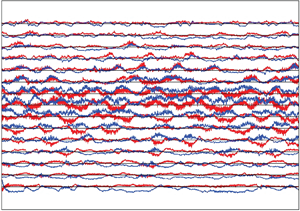
Figure 9. Longitudinal  $u_x$ (blue curves) and transverse
  $u_y$ (red curves) velocity components measured at points located along the line
  $z=0$ at
  $x=1.6 a=44\ {\rm mm}$ in flows with (a,b)
  ${{Re}}=800$,
  ${{Ha}}=200$ and (c,d)
  ${{Re}}=800$,
  ${{Ha}}=1300$. Profiles of
  $\langle u_x \rangle$ and
  $\langle u_y \rangle$ obtained by averaging over 610 s are shown in (a,c). Velocity fluctuations around the time-averaged values are shown in (b,d). In the latter, each pair of red and blue curves shows a velocity signal measured at a
  $y$-location indicated by a respective point in the left-hand-side graph. The velocity scale in (b,d) is such that the half-distance between the black lines corresponds to
  $60U_0$.

Figure 10. Time-averaged characteristics of flows at (a)  ${{Ha}}=200$,
  ${{Re}}=800$; (b)
  ${{Ha}}=1300$,
  ${{Re}}=800$; (c)
  ${{Ha}}=550$,
  ${{Re}}=5000$; and (d)
  ${{Ha}}=1300$,
  ${{Re}}=3000$. Profiles measured at
  $x=1.6a$,
  $z=0$ are shown: 1,
  $\langle u_x \rangle /U_0$; 2,
  $\langle u_y \rangle /U_0$; 3,
  $\sigma _x/U_0$; 4,
  $\sigma _y/U_0$.
Figure 8 also illustrates the existence of two clearly different states of the flow. The time-averaged velocity profiles are symmetric with respect to the centreline  $y=0$ at low Hartmann numbers, such as
  ${{Ha}}=200$ in figure 8(a). Strong asymmetry is observed at higher
  ${{Ha}}$, such as
  $Ha=1300$ in figure 8(b). The presence of an asymmetric velocity profile with a negative component almost equivalent to a positive one indicates the fact that the flow is not just the result of attaching a flat quasi-2D jet to the wall, but that there is a formation of a large recirculation zone: a macro vortex.
The two typical behaviours observed at moderate and high values of  ${{Ha}}$ are further illustrated in figure 9 on the example of flows at
  ${{Re}}=800$,
  ${{Ha}}=200$ and
  ${{Re}}=800$,
  ${{Ha}}=1300$. Time-averaged values and waveforms of longitudinal
  $u_x$ and transverse
  $u_y$ velocity components measured at points distributed along
  $y$ at
  $z=0$ are provided. The waveforms show instantaneous simultaneously measured local values of
  $u_x$ and
  $u_y$, from which time-averaged values computed at the same
  $y$ are subtracted. One should keep in mind that waveforms corresponding to different measurement points are recorded during different periods of time, so any apparent correlation between them is purely coincidental.
Figures 9(a) and 9(b) illustrate a typical flow observed at moderate values of  ${{Ha}}$. The profile of
  $\langle u_x \rangle$ is symmetric. It has a peak at
  $y=0$ and shows positive values of
  $\langle u_x \rangle$ at about
  $-10< y<10$ mm. This area coincides with the area of high-amplitude fluctuations in the waveforms. We conclude that the interval
  $-10< y<10$ mm corresponds to the zone swept by an oscillating central jet. Outside this interval, i.e. at
  $y<-10$ mm or
  $y>10$ mm,
  $\langle u_x \rangle <0$ and the amplitude of velocity fluctuations is significantly lower. These areas are identified as those of a weakly turbulent reversed flow. The picture of an expanding central jet is further confirmed by the profile of
  $\langle u_y \rangle$ shown in figure 9(a). After a correction for a zero shift we observe a flow in the positive
  $y$-direction at
  $y>0$ and in the negative
  $y$-direction at
  $y<0$.
The waveforms in figure 9(b) show strong fluctuations in the central area, especially at  $y=0$. The maximum amplitude exceeds
  $60U_0$ at some moments. The dominant frequencies correspond to the time period of about 6–7 s. There are also oscillations of much higher frequency and lower amplitude corresponding to three-dimensional turbulence. Another interesting feature is the correlation between fluctuations of
  $u_x$ and
  $u_y$ observed in the side regions of the jet but not in its centre. Positive peaks of
  $u_x$ correlate with positive or negative peaks of
  $u_y$ at, respectively,
  $y>0$ or
  $y<0$. Such events are identifiable as excursions of the jet into the areas of positive or negative
  $y$.
$y$.
An entirely different structure of the flow is presented by the measurements made at  ${{Re}}=800$,
  ${{Ha}}=1300$ (see figure 9c,d). The asymmetry, which we have already presented in figure 8, demonstrates that the jet is shifted toward one side of the duct. It must be stressed that the apparent shift is a result of time-averaging. The signal of
  $u_x$ at
  $y=a/2$ shown in figure 11 illustrates the fact that velocity fluctuates and may become negative at some moments. Once time-averaging over a sufficiently long time period is taken, however, the jet is found consistently located on one side of the duct, at positive (as in figures 10b and 9c) or negative
  $y$. No preference for one side and no spontaneous switches of the time-averaged profiles from one side to another have been found in the experiments. The possibility of such behaviours cannot be excluded, because no special studies that could detect them (statistical studies with multiple realisations of the same flow or very long measurement runs) have been completed.

Figure 11. Signal of longitudinal velocity  $u_x$ measured at
  $z=0$,
  $y=a/2$ in the flow with
  ${{Re}}=900$,
  ${{Ha}}=1300$.
The profiles of  $\langle u_x \rangle$ and
  $\langle u_y \rangle$ in figure 9(c) also show a reversed flow in the negative
  $y$ part of the duct. It is nearly as strong as the jet itself. The global structure of the asymmetric flow structure can be characterised as that of a macrovortex.
The velocity waveforms in figure 9(d) demonstrate significant fluctuations in the entire measurement region. The typical amplitude and frequency of the fluctuations are higher in the zone of the jet at positive  $y$ than in the zone of reversed flow. It can also be seen that high-frequency turbulence oscillations present in the flow at
  ${{Ha}}=200$ (see figure 9b) are not seen at
  ${{Ha}}=1300$. This is attributed to quasi-two-dimensionality of flow structures at such high
  ${{Ha}}$.
The profiles of mean velocities  $\langle u_x \rangle$,
  $\langle u_y \rangle$ and standard deviations
  $\sigma _x$,
  $\sigma _y$ (see (3.3a,b)) non-dimensionalised by the mean duct velocity
  $U_0$ are shown in figure 10. They further illustrate the existence of the two types of flow structure found in the experiments: a central jet and a macrovortex. The structure of the macrovortex becomes more complex at high
  ${{Re}}$, as illustrated by the multiple extrema of the profile of
  $\langle u_x \rangle$ in figure 10(d).
It is possible to differentiate between flow states with a central jet and a macrovortex using magnitudes of the time-averaged velocity components and their standard deviations at the central point  $y=z=0$. Results of such an analysis carried out for two values of
  ${{Re}}$ and the entire explored range of
  ${{Ha}}$ are presented in figure 12. To indicate the magnitude of velocity with respect to the mean inlet velocity of the jet
  $U_p=110U_0$, a horizontal line corresponding to
  $U_p/2$ is drawn in figures 12(a) and 12(b).

Figure 12. Velocity measurements at the center of the duct  $y=z=0$ in the cross-section
  $x=1.6a$. (a,b) Time-averaged velocity components and (c,d) standard deviations based on signals of length 600 s are shown. Here (a,c)
  ${{Re}}=800$ and (b,d)
  ${{Re}}=3000$; 1,
  $\langle u_x \rangle$ and
  $\sigma _x$; 2,
  $\langle u_y \rangle$ and
  $\sigma _y$. The horizontal dash-dotted line in (a,b) shows the value equal to half of the mean inlet velocity of the jet. The vertical solid lines indicate
  ${{Ha}}_{cr}$ separating central jet and macrovortex regimes (see the text).
The data for  $\langle u_x \rangle$,
  $\sigma _x$ and
  $\sigma _y$ (although not for
  $\langle u_y \rangle$, which is nearly zero for all
  ${{Ha}}$) clearly show the existence of two intervals of
  ${{Ha}}$ with distinct behaviours. The critical Hartmann numbers separating the intervals (shown as vertical lines in figure 12) are approximately
  ${{Ha}}_{cr}=380$ at
  ${{Re}}=800$ and
  ${{Ha}}_{cr}=780$ at
  ${{Re}}=3000$. At
  ${{Ha}}<{{Ha}}_{cr}$,
  $\langle u_x \rangle$ is large and gradually decreases from its maximum
  $\langle u_x \rangle \approx 25U_0$ at
  ${{Ha}}=200$ (as explained in § 3, this is the lowest
  ${{Ha}}$ at which accurate measurements are possible) to nearly zero. The intensity of velocity fluctuations quantified by
  $\sigma _x$ and
  $\sigma _y$ also decreases and reaches its minimum at
  ${{Ha}}={{Ha}}_{cr}$.
The interval  ${{Ha}}>{{Ha}}_{cr}$ is characterised by small values of
  $\langle u_x \rangle /U_0$ and by
  $\sigma _x$ and
  $\sigma _y$ growing with
  ${{Ha}}$ to large values (about
  $12U_0$ to
  $14U_0$). Some decrease of the standard deviation at very high
  ${{Ha}}$ is observed at
  ${{Re}}=600$ but not in the explored range of
  ${{Ha}}$ at
  ${{Re}}=1300$.
A detailed discussion of the flow transformation causing the radical change of behaviour is provided in § 5. Here we state only the evident conclusion that, in the cross-section of the duct studied in our experiments, the flow takes the form of a central jet at  ${{Ha}}<{{Ha}}_{cr}$ and of a macrovortex at
  ${{Ha}}>{{Ha}}_{cr}$.
The effect of the magnetic field on the properties of the velocity signal measured at the duct's centre is illustrated in figure 13. Properties of  $u_x$ at
  ${{Re}}=800$ and
  ${{Ha}}=200$ (central jet),
  ${{Ha}}=1000$ (macrovortex) and
  ${{Ha}}=350$ (close to
  ${{Ha}}_{cr}$) are shown. We see the typical features of flow transformation observed in other MHD flows in experiments and numerical simulations, e.g. by Kolesnikov & Tsinober (Reference Kolesnikov and Tsinober1972), Alemany et al. (Reference Alemany, Moreau, Sulem and Frisch1979), Burattini, Zikanov & Knaepen (Reference Burattini, Zikanov and Knaepen2010), Verma (Reference Verma2017) and Zikanov et al. (Reference Zikanov, Krasnov, Boeck and Sukoriansky2019). The transition into a quasi-2D form at growing
  ${{Ha}}$ is associated with suppression of high-frequency fluctuations, growth of energy of low-frequency fluctuations and steeper energy spectra with the slope approaching
  ${\sim }f^{-3}$ (see figure 13a,b). The signal is also shown using its standard deviation averaged over a sliding 15-second interval (figure 13c).

Figure 13. Properties of the signal of longitudinal velocity  $u_x$ measured at the centre
  $y=z=0$ of the duct in the cross-section
  $x=1.6a$ at
  ${{Re}}=800$ and
  ${{Ha}}=200$, 350 and 1000. (a) Signals in a 15 s window. (b) Power spectral density based on 600 s of observations. The apparent peaks at
  $f=50$ Hz are caused by interference from the power supplies. The slopes
  ${\sim }f^{-5/3}$ and
  ${\sim }f^{-3}$ are shown for guidance. (c) Curves of the standard deviation calculated in a moving 15 s window.
The typical amplitude of velocity oscillations varies non-uniformly with  ${{Ha}}$. It decreases from about
  $10U_0$ to about
  $5U_0$ when
  ${{Ha}}$ changes from 200 to 350 and increases back to about
  $10U_0$ when
  ${{Ha}}$ increases to 1000.
The results of all the reported measurements of longitudinal velocity at the duct centre are summarised in figure 14. Mean value and standard deviation (3.3a,b) of the longitudinal velocity  $u_x$ scaled with
  $U_0$ are shown as functions of
  ${{N}}$ in figures 14(a) and 14(b). Dimensionless skewness and kurtosis
 \begin{equation} b_{1}=\frac{\langle(u_x-\langle u_x\rangle)^3\rangle}{\sigma_x^3}, \quad g_2=\frac{\langle(u_x-\langle u_x\rangle)^4\rangle}{\sigma_x^4} \end{equation}
are shown in figures 14(c) and 14(d).

Figure 14. (a) Non-dimensionalised mean value  $\langle u_x \rangle$, (b) standard deviation
  $\sigma _x$, (c) skewness and (d) kurtosis of longitudinal velocity measured at the duct centre
  $y=z=0$ versus the Stuart number
  ${{N}}$. Data for the cross-sections
  $x=1.6a$ (I and II) and
  $x=5.2a$ (II-a) are shown. Measurements series I and II are performed using sensors of type 1 and 2, respectively, shown in figures 4(a) and 4(b). Measurements of series II-a are performed using a sensor similar to the sensor of type 2 in its design (see § 3.3).
We see that the two trends presented by figure 12 are universal. The mean centreline velocity decreases with the increasing strength of the magnetic field effect and becomes small when the field is strong (see figure 14a). The amplitude of the fluctuations has two maxima, one at small and one at large  ${{N}}$, and a minimum at intermediate values of
  ${{N}}$. The minimum is clearly identifiable in experiments at all values of
  ${{Re}}$, although it is more pronounced at small Reynolds numbers.
The line  $\langle u_x\rangle \sim {{N}}^{-0.5}$ in figure 14(a) corresponds to the theoretically determined MHD decay of velocity in a submerged uniform jet in an infinite domain (Davidson Reference Davidson1995). It is not surprising that the experimental data do not reproduce this slope closely. The real jet is spatially evolving rather than uniform and occurs in a bounded domain of the duct.
We now analyse the data in figure 14 in conjunction with the results presented earlier, attempting to form a unifying picture of flow's transformation caused by the magnetic field. The first observation concerns the role of the Stuart number  ${{N}}$ as a key non-dimensional parameter determining the flow state. We see in figure 14(b) that all the data collected in the cross-section
  $x=1.6a$ at various values of
  ${{Re}}$ and using sensors of two different types collapse into one curve. The amplitude of the fluctuations is determined by
  ${{N}}$ as a single parameter. A similar behaviour, albeit with stronger uncertainty, is observed for the higher statistical moments: skewness and kurtosis shown in figures 14(c) and 14(d). The situation is more complex for the mean velocity. One may argue that the decay of
  $\langle u_x\rangle$ at
  ${{N}}<170$ is still largely determined by the value of
  ${{N}}$. The small values of
  $\langle u_x\rangle$ at
  ${{N}}>170$ do not follow a clear trend. This can be related to insufficient averaging time in the experiments. The signal in figure 11 indicates flow dynamics that may require much longer than 600 s to measure true average values. Another possible explanation is the effect of Hartmann boundary layers, which are not uniquely identified by
  ${{N}}$.
Considering  ${{N}}$ as a control parameter and using the data in figure 14, we can identify four distinct zones characterised by different behaviours.
In zone 1, at approximately  ${{N}}<50$, the fluctuation amplitude increases and the mean velocity decreases with
  ${{N}}$. The normalised standard deviation reaches the peak of
  $\sigma _x\approx 15U_0$ at
  ${{N}}=50$. The skewness coefficient
  $b_1$ is negative, indicating intrusion of slow fluid particles into the axial region. The values of the kurtosis coefficient are close to those of a normal distribution.
Zone 2 at  $50<{{N}}<170$ is characterised by a decrease of the mean velocity, with a rate higher than in zone 1. The fluctuation intensity
  $\sigma _x$ decreases with
  ${{N}}$ at a rate of about
  $\sigma _x \sim {{N}}^{-0.5}$. The smallest values of the fluctuation amplitude are observed at
  ${{N}}=170$. Skewness increases with
  ${{N}}$ and becomes significantly positive. Kurtosis also increases and becomes noticeably larger than the normal distribution value. We see that while decreasing in amplitude, velocity fluctuations in the area of the duct's axis become increasingly dominated by fluid particles strongly accelerated in the positive
  $x$-direction.
Interestingly, the lower boundary  ${{N}}=50$ of zone 2 corresponds at the same time to the maximum of the fluctuation amplitude
  $\sigma _x$, nearly zero skewness
  $b_1$ and minimum kurtosis
  $g_2$. The upper boundary
  ${{N}}=170$ represents an entirely different state of the flow, in which
  $\sigma _x$ is at its minimum and
  $b_1$ and
  $g_2$ reach their maximum values.
In zone 3, defined approximately as  $170<{{N}}<1200$, the fluctuation amplitude grows again, initially as
  $\sigma _x \sim {{N}}^{0.5}$ and then at a slower rate. Skewness and kurtosis decrease, both remaining above the normal distribution values. This indicates continuing dominance of fluctuations with excess streamwise velocity.
We can also identify zone 4 at  ${{N}}>1200$, where the local mean velocity at the duct axis
  $u_x(y=0,z=0)$ approaches the value of the mean velocity in the duct
  $U_0$. All three statistical moments indicate the persistence of velocity fluctuations with a strong positive streamwise component.
It should be stressed that the just-described universal behaviour is found in the cross-section  $x=1.6a$ but not in the cross-section
  $x=5.2a$ further downstream. We hypothesise that the effect of
  ${{Re}}$ on flow decay becomes significant at that location, so the flow state cannot be uniquely determined by
  ${{N}}$ alone.
Typical slopes  $n$ of the energy power spectra calculated for the streamwise velocity signals at
  $x=1.6a$ are shown in figure 15(a). To evaluate the slopes, time-averaged spectra are first obtained by linearly averaging 10 spectra computed using the Bartlett–Hanning window within one flow realisation. As illustrated by the examples in figure 15(b), the resolution limitations of the sensor and the short range of active frequencies related to the effect of a magnetic field on flows at moderate
  ${{Re}}$ do not allow us to evaluate the true inertial-range slope. Instead, a ‘typical’ slope is computed by bisquare fitting of the spectrum in the range between 3 and 80 Hz. It is therefore not surprising to see in figure 15(a) some values of
  $n$ lying outside the interval between
  $-3$ and
  $-5/3$ anticipated for the inertial range. Nevertheless, figure 15 presents useful information, especially if we exclude the values at the lowest and highest
  ${{N}}$. We see that the typical slope is largely determined by
  ${{N}}$ as a single non-dimensional parameter. There is a gradual decrease in
  $n$ from values around
  $-5/3$ typical for three dimensional flows at small
  ${{N}}$ to values around
  $-3$ expected for quasi-2D flows at high
  ${{N}}$. Interestingly, the decrease follows
  $n\sim \log (N^{-1})$, shown by the straight line in figure 15(a).

Figure 15. Typical slopes of the energy power spectra determined for the streamwise velocity signals measured by sensor of type 2 at  $x=1.6a$. The slopes are evaluated using bisquare fitting in the frequency range 3 to 80 Hz, as illustrated by the two subplots. In the subplots, the evaluated typical slope is presented by the red line, and the slopes
  ${\sim }\omega ^{-5/3}$ and
  ${\sim }\omega ^{-3}$ are shown for comparison.
5. Discussion and concluding remarks
In this section we attempt an explanation of the experimental results. Concluding remarks and suggestions for future work are provided at the end.
One important and evident conclusion of the experiments is that the classical picture of the transformation of a round jet in a transverse magnetic field as illustrated in figures 2 and 3 can be improved. The theoretical arguments on which the picture is based fail to predict the emergence of high-amplitude velocity fluctuations and modification of the mean velocity profile found at high Stuart numbers.
Another outcome of the experiment, namely that some flow properties are accurately described by a function of  ${{N}}$ as a single parameter, is not surprising. The jet instability in the presence of a strong magnetic field is anticipated to be determined mainly by the ratio between the Lorentz and inertial forces, which is estimated by
  ${{N}}$. The key mechanisms determining the flow evolution are the Kelvin–Helmholtz instability of the jet, the transition of the flow into a quasi-2D state, the Joule damping of velocity fluctuations and the Hartmann friction. Viscous dissipation is less significant in flows with such high
  ${{Ha}}$ and
  ${{Re}}$. It is ignored in the following discussion.
The jet instability is strong because of high  ${{Re}}$ and additional perturbations introduced near the inlet by the Lorentz force in the form of transverse velocity components associated with the transformation into anisotropic form (in that way, the instability can be enhanced rather than suppressed by the magnetic field). The presence of high-amplitude fluctuations at a distance of 44 mm, i.e. about seven jet diameters, from the inlet is therefore not surprising.
The Joule dissipation of velocity fluctuations is strong if the fluctuations are significantly three-dimensional but vanishes when the flow approaches quasi-2D form. The damping effect due to friction in Hartmann layers appears in quasi-2D flows, but it is generally weaker. These arguments have been demonstrated earlier to be a valid explanation of the so-called residual fluctuations (see, e.g., Kolesnikov & Tsinober Reference Kolesnikov and Tsinober1972; Sukoriansky, Zilberman & Branover Reference Sukoriansky, Zilberman and Branover1986; Zikanov et al. Reference Zikanov, Krasnov, Boeck and Sukoriansky2019): high-amplitude low-frequency oscillations of velocity that appear in shear flows at high values of  ${{N}}$.
One may consider this phenomenon as a manifestation of the general effect of vortex reorganisation by a magnetic field, found prominently in various turbulent or fluctuating flows. This phenomenon has been studied experimentally and theoretically by many authors since the 1970s. Experimental works by Eckert et al. (Reference Eckert, Gerbeth, Witke and Langenbrunner2001) and Bühler, Horanyi & Arbogast (Reference Bühler, Horanyi and Arbogast2007) provide a detailed analysis of two-dimensional phenomena and changes in the flow intensity for a duct in a transverse field. Experiments of Pothérat & Klein (Reference Pothérat and Klein2014, Reference Pothérat and Klein2017), where the emergence of a system of anisotropic vortices in a cube is artificially forced by supplying electric current through the wall in the presence of a magnetic field, whereas only indirectly related to our study, nevertheless provide information about the effects of the interaction of a system of anisotropic vortex structures. Similar effects have been considered in the context of Rayleigh–Bénard convection (Vogt et al. Reference Vogt, Ishimi, Yanagisawa, Tasaka, Sakuraba and Eckert2018). Thermal convection (Zikanov et al. Reference Zikanov, Belyaev, Listratov, Frick, Razuvanov and Sviridov2021) can lead to emergence of high-amplitude unsteady structures when conventional turbulence is suppressed by the magnetic field and the flow becomes quasi-2D. The results of all these studies are consistent with our conclusions. They demonstrate the ability of an applied magnetic field not only to suppress velocity fluctuations, but also to generate fluctuations of a peculiar large-scale quasi-2D nature.
We now attempt to reconstruct, based on incomplete data, the flow transformation represented by the results shown in figures 8–15. A sketch illustrating the discussion is provided in figure 16.

Figure 16. Sketch of the typical flow structures at various values of Stuart number: (a) is based on results of Anghan et al. (Reference Anghan, Dave, Saincher and Banerjee2019) and (b,c) are based on experimental data.
In zones 1 and 2, at approximately  ${{N}}<170$, the mean flow has a central jet (see figure 16b). The centreline velocity decreases with increasing
  ${{N}}$. The typical amplitude of centreline velocity fluctuations increases with
  ${{N}}$ in zone 1 and decreases with
  ${{N}}$ in zone 2. The flow is anisotropic but still not quasi-2D (see figure 8a). We hypothesise that the dominant effect of the magnetic field in zone 1 is the effect consistent with both observed trends, namely, destabilisation of the jet by the Lorentz force. A similarly consistent dominant effect in zone 2 is the suppression of three-dimensional velocity fluctuations by the Joule dissipation. In other words, zone 1 corresponds to the situation in which the unstable three-dimensional perturbations are still growing in the measurement cross-section. Zone 2 corresponds to the situation in which the magnetic field is stronger and the growth has already been replaced by dissipation-caused decay by the time the fluid arrived at the measurement site. The skewness and kurtosis data in figure 14 suggest that the surviving fluctuations are dominated by structures with high streamwise velocity.
The sharp minimum of the fluctuation amplitude at the boundary  ${{N}}=170$ between zones 2 and 3 indicates that the flow undergoes a radical transformation. We hypothesise that zones 3 and 4 correspond to quasi-2D flow states in the measurement cross-section. The central jet does no longer exist in this cross-section. As illustrated in figure 16(c), the jet is diverted to one side of the duct, forming a quasi-2D macrovortex. The mean velocity at the centreline is nearly zero. The amplitude of velocity fluctuations increases with
  ${{N}}$ in zone 3 and decreases with
  ${{N}}$ in zone 4. It must be stressed that the nature of velocity fluctuations is completely different from the nature of fluctuations in zones 1 and 2. As illustrated in figures 13 and 15, they are characterised by a steep slope of the energy power spectrum and dominance of low-frequency oscillations. The only plausible explanation for the emergence of such fluctuations at high
  ${{N}}$ is that they are caused by large-scale unsteady quasi-2D structures associated with shear-flow instability of a macrovortex. The increase of the fluctuation amplitude with
  ${{N}}$ in zone 3 can be explained by a combination of two effects promoting the growth of such structures: stronger quasi-two-dimensionality and the shift of the jet-to-vortex transition upstream. The decrease of the fluctuation amplitude in zone 4 is attributed to the effect of growing friction in the Hartmann boundary layers.
It is known that, generally, a central jet diverts towards a wall and forms a large-scale vortex (see, e.g., Escudier, Oliveira & Poole Reference Escudier, Oliveira and Poole2002). It is found in this study that the process is dramatically changed by an applied magnetic field. The anticipated effects of stabilisation and quasi-two-dimensionality of the vortex are observed. At the same time, the process is found to be much more complex, involving a multi-stage transformation with growing Stuart number and high-amplitude velocity fluctuations reappearing at strong magnetic fields.
The experimental results are presented in this paper for a broad range of parameters. This allows us to analyse the effect of the magnetic field and identify distinct modes of the flow's behaviour. At the same time, the experimental data are inevitably limited in the sense that they do not produce a complete picture of the flow. Many aspects of the explanation proposed in this section must therefore be viewed as hypothetical until confirmation in the form of numerical simulation data is available. Such simulations are a necessary and logical next step of the analysis. Their goals are (i) to produce detailed descriptions of various states of the flow and (ii) to provide data for a quantitative analysis based on a detailed comparison between the experimental and numerical data. Preliminary results of numerical simulations confirming existence of the two principally different flow states are provided in the Appendix of this paper.
As a final comment, we would like to stress that the conclusions are rigorously valid only in the case presented in this paper: a jet bounded by duct walls on the sides and by the junction between pipe and duct in the inlet plane. The behaviour would be different for a jet issued into an unbounded domain. It might also be different if, in the presence of duct walls, the junction were replaced by a low-velocity inlet, although we believe that this would not qualitatively affect the key features of the flow, such as formation of a macro-vortex. Our results are, therefore, only indirectly related to the theoretical results on expansion of a jet into an unbounded domain, such as those of Davidson (Reference Davidson1995). The relation is more direct to works on sudden expansion (Mistrangelo Reference Mistrangelo2006; Mistrangelo & Bühler Reference Mistrangelo and Bühler2007; Mistrangelo Reference Mistrangelo2011), and to practical applications, such as liquid metal blankets for fusion reactors and continuous steel casting, for which the effect of side wall and pipe to duct junction is an inherent part. We also note that a significant effect of walls, especially of the Hartmann walls, is an inherent feature of high-field magnetohydrodynamics.
Funding
The work of I.B., N.L., Y.L., O.Z. and experimental methods development were supported by the award 20-69-46067 from the Russian Science Foundation. The work of I.M. and experimental facility maintenance were supported by the Ministry of Science and Higher Education of the Russian Federation (State Assignment Number 075-01056-22-00). Computational time for the numerical simulations presented in the Appendix was provided by the Leibniz Supercomputing Centre on the SuperMUC-NG super-computing cluster (project pn68ni). Visualisations of the computed flow fields were performed at the University Computing Centre of the TU Ilmenau. Authors are grateful to reviewers for careful reading of the manuscript and constructive comments.
Declaration of interests
The authors report no conflict of interest.
Appendix
Results of preliminary direct numerical simulations are briefly presented here. Flows at  ${{Re}}=1000$,
  ${{Ha}}=100$ and
  ${{Re}}=1000$,
  ${{Ha}}=1000$ are computed as typical representatives of low-
 ${{N}}$ and high-
 ${{N}}$ regimes. The simulations are performed in long computational domains on computational grids consisting of
  $2304\times 384^2$ grid points. The numerical scheme described in our earlier works, such as Krasnov et al. (Reference Krasnov, Listratov, Kolesnikov, Belyaev, Pyatnitskaya, Sviridov and Zikanov2021) and Zikanov et al. (Reference Zikanov, Krasnov, Boeck and Sukoriansky2019), is used. Further details of the numerical procedure will be provided in a future publication by the authors of this paper.
The instantaneous distributions of the streamwise velocity shown in figure 17 confirm the main conclusion of the experiment. The flow structure is dominated by a fluctuating central jet at low  ${{N}}$ and by a macrovortex attached to one of the sidewalls at high
  ${{N}}$.

Figure 17. Results of preliminary numerical simulations. Instantaneous distributions of axial velocity in the duct cross-section perpendicular to the magnetic field are shown for: (a)  ${{Re}}=1000$,
  ${{Ha}}=100$,
  ${{N}}=10$; (b)
  ${{Re}}=1000$,
  ${{Ha}}=1000$,
  ${{N}}=1000$. The velocity is non-dimensionalised by the mean velocity in the duct. The red dashed line indicates the cross-section, where the measurements are done in the experiment.


