


1. Introduction
The appearance of bedforms on granular beds has been studied for many years; Charru, Andreotti & Claudin (Reference Charru, Andreotti and Claudin2013) have recently presented a summary of these works. The specific structurations of stratified particles, which appear when the threshold of motion is reached, can be obtained under various flow conditions. For example, they can be observed under continuous flow in closed geometries (Kuru, Leighton & McCready Reference Kuru, Leighton and McCready1995; Wierschem et al. Reference Wierschem, Groh, Rehberg, Aksel and Kruelle2008), in open channel flow (Friedrich et al. Reference Friedrich, Coleman, Melville and Clunie2004), and under oscillating flows, caused for instance by sea surface waves (Blondeaux Reference Blondeaux1990).
For continuous flows, the appearance of bedforms, from an initial uniform flat bed, is not clearly understood. The most advanced theory to explain the growth of an initial instability is the spatial shift between the bedforms and the particle flux generated by the wall shear stress. This theory was first proposed by Kennedy (Reference Kennedy1963). Based on this idea, many models of linear stability analysis, starting with Engelund (Reference Engelund1970), have been suggested to explain the development of the initial wavelets. The variety of correlations proposed to calculate the solid flux as a function of the Shields number explains the large number of current models. Charru has worked on this subject extensively and clearly explains the different models in Charru & Hinch (Reference Charru and Hinch2006a ,Reference Charru and Hinch b ).
Experimental results have shown that turbulence is not at the origin of the bedform patterns since it can be observed in laminar flows (Kuru et al. Reference Kuru, Leighton and McCready1995; Coleman & Eling Reference Coleman and Eling2000). In a finite size flume, with a continuous flow without free surface interaction, the evolution of bedforms, starting with a flat bed, can typically be divided into three stages (Coleman & Eling Reference Coleman and Eling2000; Rauen, Lin & Falconer Reference Rauen, Lin and Falconer2008), during which the form and size of bedforms evolve in time and space.
-
(i) Appearance of initial wavelets: when the first particles are set in motion, the fluid stream can shape the granular bed by erosion. Depending on the flow characteristics, instability in the stream flow can lead to the formation of an initial wavy bed surface. This first deformation is transverse to the main flow, small, smooth, regularly spaced on the bed surface, and propagates slowly downstream. This stage has been widely studied experimentally and numerically. Many empirical correlations have been proposed in the past few years to determine the initial wavelength for different duct geometries and particle characteristics (Yalin Reference Yalin1977, Reference Yalin1985; Kuru et al. Reference Kuru, Leighton and McCready1995; Coleman & Melville Reference Coleman and Melville1996; Raudkivi Reference Raudkivi1997; Coleman & Eling Reference Coleman and Eling2000).
-
(ii) Shape transition: initial wavelets grow with time (and/or in space), increasing their amplitude until they mutate into ripples. This transition is triggered when the amplitude of the initial wavelets becomes too high. The stream flow can no longer follow the bed surface and a detachment point is formed after the crest of the wavelet. A vortex of recirculation is thus generated in the downstream flow. The smooth wavelet shape changes to a form called vortex ripples. The bedforms obtained are still transverse to the main flow and propagate in the flow direction.
Rauen et al. (Reference Rauen, Lin and Falconer2008) studied this transition with fine silica sand (
 $d=130~{\rm\mu}\text{m}$
) under a continuous turbulent water flow in a laboratory flume 30 cm in width. They determined, for their open channel flow, that the transition occurs when the ripple steepness,
${\it\eta}=L/H$
, exceeds a critical value depending on the grain diameter.
$d=130~{\rm\mu}\text{m}$
) under a continuous turbulent water flow in a laboratory flume 30 cm in width. They determined, for their open channel flow, that the transition occurs when the ripple steepness,
${\it\eta}=L/H$
, exceeds a critical value depending on the grain diameter.Vortex ripples, like wavelets, are two-dimensional bedforms transverse to the direction of the flow. However if the stream flow is too high, another instability can appear, breaking the ripple regularity in the third direction. Three-dimensional bedforms, often termed dunes to differentiate them, are thus generated. Depending on the channel geometry (closed channel, open flow), different dunes can be observed. In circular pipes, experimental observations have shown that this transversal instability leads to only one specific bedform: sinuous dunes (Kuru et al. Reference Kuru, Leighton and McCready1995; Ouriemi, Aussillous & Guazzelli Reference Ouriemi, Aussillous and Guazzelli2009).
During this period of transition, the characteristics of ripples and dunes are constantly changing: their shape, size and the length between each bedform are growing. Smaller bedforms can collapse to leave space for others or merge to form bigger ones. As the bedforms observed are highly dependent on time and the initial conditions, their characterisation is difficult. Depending on experimental parameters, this stage can take from a few minutes to days.
-
(iii) Saturation: if the solid flux can be maintained constant over a long period of time, the characteristics of ripples reach a threshold value and become constant in time and space. This state corresponds to the saturated profile of bedforms. Vortex ripples can then be modelled by the equation of transversal propagating waves:
(1.1)where
$$\begin{eqnarray}h(x,t)=h_{0}+A_{sat}\cdot f\left(\frac{t}{T_{sat}}+\frac{z}{{\it\lambda}_{sat}}+{\it\varphi}\right)\end{eqnarray}$$
$h$
is the height of the bed,
$h_{0}$
the minimum bed height,
$z$
the longitudinal coordinate,
$t$
the time,
$T_{sat}$
the ripple period,
${\it\lambda}_{sat}$
the ripple wavelength,
${\it\varphi}$
a possible phase shift and
$f$
a specific unitary periodic function related to the shape of bedforms.
This state must not be confused with the equilibrium profile of bedforms obtained when an initial particle bed is eroded without solid feeding. In that case, the particle flux decreases with time, slowing down the progression of bedforms, which finally stop in a frozen state.
Experimentally, the difficulty of studying the saturated stage lies in the time needed to reach this equilibrium. This explains why, to the best of our knowledge, almost all previous experiments have been carried out on sediment particle beds without solid feeding to compensate for the erosion (Coleman & Eling Reference Coleman and Eling2000; Ouriemi et al. Reference Ouriemi, Aussillous and Guazzelli2009).
The saturated state was studied by Raudkivi (Reference Raudkivi1997) who observed that geometrical characteristics depend on the size of the grain, with finer sediments tending to produce steeper bedforms (the wavelength growing faster than the amplitude with an increase in grain diameter), and that flow conditions have no influence on them.
Doppler et al. (Reference Doppler, Loiseleux, Gondret and Rabaud2004) studied the influence of the tilt angle in a Hele-Shaw flume with glass beads of 112 and
$132~{\rm\mu}\text{m}$
. They observed that the phase velocity exhibits a weak dependence on the tilt angle and the flow rate, but is strongly influenced by the grain diameter.Andreotti, Claudin & Pouliquen (Reference Andreotti, Claudin and Pouliquen2006) studied aeolian saturated sand ripples in a wind tunnel (
$d=140~{\rm\mu}\text{m}$
). They found that the ripple propagation velocity, starting from zero at the threshold of motion, increases linearly with the bed shear velocity.To the best of the authors’ knowledge, no study has focused on saturated bedforms in circular pipes.


This work on ripple characterisation was undertaken with the aim of studying the flow of ice slurry in pipes. Ice slurries (Kauffeld, Kawaji & Egolf Reference Kauffeld, Kawaji and Egolf2005) are solid–liquid phase change materials, used as a secondary coolant in refrigerated systems. In this application, the low density of ice, compared with the carrier fluid, may result in the stratification of the ice particles in pipes. It is therefore important to control the phenomena occurring with the stratification. In order to study the flow of such a stratifying mixture without heat transfer and transport of species, we worked with a mixture of water and polypropylene particles, which have characteristics (density, sizes) close to those of ice crystals present in ice slurries. Mimicking ice crystals was thus the main reason for investigating flows where particles are floating, a case that has never been dealt with in the study of bedforms. Ripple formation and propagation, although not of direct industrial interest, must be controlled to avoid breakdowns. Sediment transport in pipes is also subject to this phenomenon, as stated by Matousek & Krupicka (Reference Matousek and Krupicka2013).
The experimental set-up, presented in § 2.1, provided an infinite recirculation of a mixture of water and solid particles and enabled bedforms to be observed, over a long period, in a saturated state. Three different ways of determining bedform characteristics were explored and are presented in §§ 2.2 and 2.3. The flow patterns observed are explained in § 3.1, where the threshold of motion is discussed. The development of the bedforms obtained and a verification of their stability are reported in § 3.2. Finally, the results of the different analyses are given and discussed in § 3.3.
2. Experimental methodology
2.1. Experimental set-up
The experiments reported herein were carried out in a 4-m-long horizontal circular tube made of transparent PMMA, with an inner diameter
 $D=3~\text{cm}$
(figure 1). The multistage centrifugal pump (Grundfos CHV2) circulating the flow was controlled using a variable speed drive in order to vary the flow rate. The minimum space of the free section inside the pump was 3 mm, large enough to allow the flow of particles of less than 1 mm. As a result, the mixture of water and particles was recirculated without any problem. The solid load
$D=3~\text{cm}$
(figure 1). The multistage centrifugal pump (Grundfos CHV2) circulating the flow was controlled using a variable speed drive in order to vary the flow rate. The minimum space of the free section inside the pump was 3 mm, large enough to allow the flow of particles of less than 1 mm. As a result, the mixture of water and particles was recirculated without any problem. The solid load
 ${\rm\Phi}$
(ratio of the volume of solid over the total volume of the set-up, corresponding to the solid concentration) was regulated by a special apparatus enabling a specific quantity of solid to be added to the loop. The protocols used, detailed in § 3.2.2, provided uniformity in the dispersion of the solid in the set-up at the beginning of each test. The use of a constant diameter in the set-up leads to substantially similar flow conditions everywhere in the closed loop (very low localised accumulation of solid). The combination of these two conditions means that
${\rm\Phi}$
(ratio of the volume of solid over the total volume of the set-up, corresponding to the solid concentration) was regulated by a special apparatus enabling a specific quantity of solid to be added to the loop. The protocols used, detailed in § 3.2.2, provided uniformity in the dispersion of the solid in the set-up at the beginning of each test. The use of a constant diameter in the set-up leads to substantially similar flow conditions everywhere in the closed loop (very low localised accumulation of solid). The combination of these two conditions means that
 ${\rm\Phi}$
can be considered constant, in a first approximation, in the set-up.
${\rm\Phi}$
can be considered constant, in a first approximation, in the set-up.

Figure 1. Schematic of the experimental set-up.
A Coriolis mass flow meter (E+H Promass 83I) was used to measure the mass flow rate (
 ${\dot{m}}_{m}$
) and the density of the mixture (
${\dot{m}}_{m}$
) and the density of the mixture (
 ${\it\rho}_{m}$
). The pipe, the pump and the flow meter were connected to each other by hoses of 30 mm. By ensuring the continuity of the cross-section throughout the loop, and by recirculating the particles, the condition at the tube inlet of the tube could be considered the outlet condition. The solid flux corresponded, continuously, to the saturated flux as explained in Andreotti, Claudin & Pouliquen (Reference Andreotti, Claudin and Pouliquen2010). A stable state could be maintained indefinitely and saturated ripples could thus be studied.
${\it\rho}_{m}$
). The pipe, the pump and the flow meter were connected to each other by hoses of 30 mm. By ensuring the continuity of the cross-section throughout the loop, and by recirculating the particles, the condition at the tube inlet of the tube could be considered the outlet condition. The solid flux corresponded, continuously, to the saturated flux as explained in Andreotti, Claudin & Pouliquen (Reference Andreotti, Claudin and Pouliquen2010). A stable state could be maintained indefinitely and saturated ripples could thus be studied.
The fluid used as the carrier phase was water maintained at room temperature (
 $24\pm 1.5\,^{\circ }\text{C}$
). The viscosity and density were deduced from the table of water characteristics:
$24\pm 1.5\,^{\circ }\text{C}$
). The viscosity and density were deduced from the table of water characteristics:
 ${\it\rho}_{l}=997\pm 1~\text{kg}~\text{m}^{-3}$
and
${\it\rho}_{l}=997\pm 1~\text{kg}~\text{m}^{-3}$
and
 ${\it\mu}_{l}=0.91\pm 0.04~\text{mPa}~\text{s}$
.
${\it\mu}_{l}=0.91\pm 0.04~\text{mPa}~\text{s}$
.
The mixture was introduced with care in order to limit the amount of air injected into the set-up. The device was then heated to
 $45\,^{\circ }\text{C}$
temporarily and its pressure lowered to 1 bar (whereas tests were carried out at 2 bars) to ensure a very low solubility of air in water. Most air bubbles were then discharged through a vent. The small amount of air not removed by this procedure dissolved completely when the test conditions were established, and it was verified visually that even very small air bubbles attached to particles disappeared.
$45\,^{\circ }\text{C}$
temporarily and its pressure lowered to 1 bar (whereas tests were carried out at 2 bars) to ensure a very low solubility of air in water. Most air bubbles were then discharged through a vent. The small amount of air not removed by this procedure dissolved completely when the test conditions were established, and it was verified visually that even very small air bubbles attached to particles disappeared.
The solid phase was composed of black particles of polypropylene, selected for their size and density. The density was measured by a helium pycnometer (Accupyc 1330) and was found to be
 ${\it\rho}_{s}=907\pm 1~\text{kg}~\text{m}^{-3}$
. To reduce polydispersion, the particles were sieved. Then, the dispersion of the particle diameters was measured by a laser particle sizer (Malvern Mastersizer 2000):
${\it\rho}_{s}=907\pm 1~\text{kg}~\text{m}^{-3}$
. To reduce polydispersion, the particles were sieved. Then, the dispersion of the particle diameters was measured by a laser particle sizer (Malvern Mastersizer 2000):
 $d_{50}=756~{\rm\mu}\text{m}$
;
$d_{50}=756~{\rm\mu}\text{m}$
;
 $d_{10}=559~{\rm\mu}\text{m}$
;
$d_{10}=559~{\rm\mu}\text{m}$
;
 $d_{90}=889~{\rm\mu}\text{m}$
. Diameters were checked after hours of recirculation, and no deterioration was detected.
$d_{90}=889~{\rm\mu}\text{m}$
. Diameters were checked after hours of recirculation, and no deterioration was detected.
This study was limited to flows obtained for
 $\mathit{Re}_{pipe}<1.5\times 10^{4}$
, where
$\mathit{Re}_{pipe}<1.5\times 10^{4}$
, where
 $\mathit{Re}_{pipe}=4{\dot{m}}_{m}/({\it\mu}_{l}{\rm\pi}D)$
, and
$\mathit{Re}_{pipe}=4{\dot{m}}_{m}/({\it\mu}_{l}{\rm\pi}D)$
, and
 ${\rm\Phi}\leqslant 0.2$
. The transition towards turbulence, for pure water, occurred for
${\rm\Phi}\leqslant 0.2$
. The transition towards turbulence, for pure water, occurred for
 $\mathit{Re}_{pipe}\approx 2300$
.
$\mathit{Re}_{pipe}\approx 2300$
.
2.2. Image processing
A CCD camera (Point Grey Chameleon) was installed at the height of the tube to observe the bedforms. To improve the contrast between bedforms (opaque stack) and the flow (transparent), retro-lights were applied on the opposite side of the camera (figure 2). The width of the zone observed was approximately 30 cm. The frames were recorded with a period of 4 s. The spatial resolution was
 $250~{\rm\mu}\text{m}$
. Examples of images obtained are shown in figure 3. By image processing the granular interface was extracted and the bed height
$250~{\rm\mu}\text{m}$
. Examples of images obtained are shown in figure 3. By image processing the granular interface was extracted and the bed height
 $h(z,t)$
calculated.
$h(z,t)$
calculated.

Figure 2. Video acquisition set-up.

Figure 3. Photographs of saturated ripples for
 ${\rm\Phi}=0.05$
, illustrating the gradual extinction of bedforms with an increase in the flow rate.
${\rm\Phi}=0.05$
, illustrating the gradual extinction of bedforms with an increase in the flow rate.
This experimental technique was previously tested by Doppler et al. (Reference Doppler, Gondret, Loiseleux, Meyer and Rabaud2007) and gave good results. Other experimental techniques are available, such as those used by Ouriemi et al. (Reference Ouriemi, Aussillous and Guazzelli2009) and Langlois & Valance (Reference Langlois and Valance2007) exploiting the deformation of a laser sheet projected obliquely onto the granular interface or the Doppler systems used by Rauen et al. (Reference Rauen, Lin and Falconer2008) and Ha & Chough (Reference Ha and Chough2003). The circular shape of the pipe induces a distortion of the light due to refraction. This deformation was estimated using a machined bed profile. For bed heights lower than
 $D/2$
, no distortion was observed, thus the amplitudes calculated for
$D/2$
, no distortion was observed, thus the amplitudes calculated for
 ${\rm\Phi}>0.05$
were not used. It should be remembered that there was no deformation in the longitudinal direction.
${\rm\Phi}>0.05$
were not used. It should be remembered that there was no deformation in the longitudinal direction.
Bed heights were compiled to construct space–time diagrams (ST-D) (figure 5) representing the evolution in time and space of the bedforms. From these data, different methods of analysis were used to determine the characteristics of the ripples.
-
(i) A Lagrangian tracking of bedforms was used to determined wavelengths (
${\it\lambda}_{sat}$
), frequencies (
$F_{Im\text{-}LAG}$
) and velocities of propagation (
$C_{sat}$
). -
(ii) Based on Fourier transforms, wavelets transforms (Torrence & Compo Reference Torrence and Compo1998; Farge Reference Farge1992) were used to identify the saturated state and its stability in time (figure 9 c). Then, time power spectral densities (PSD) were used to determine bedform frequencies (
$F_{Im\text{-}PSD}$
). Spatial PSD could be used to determine the wavelength, but this was not possible for our data, as the bedform wavelengths obtained were too long compared with the width of the area observed.


2.3. Differential pressure processing
The first 2.9 m of the horizontal pipe ensured the hydraulic establishment of the flow, for laminar as well as turbulent flow, in accordance with the usual correlations. The pressure drop in the last metre was recorded at 2 Hz by a piezoresistive manometer sensor (E+H Deltabar S PMD75) with an accuracy of 1.5 Pa.
When there is no bedform (i.e. for flat bed flows and fully suspended flows), the differential pressure measured corresponds to the pressure drop: the energy lost by the fluid in friction along the pipe. In the case of bedforms, this direct relationship is not true. In fact, at a given space point, the height of the bed will change with time. This variation in the bed height will cause a variation in the mean fluid velocity (due to the mass flow rate conservation). This evolution of the fluid velocity induces a variation in pressure, as explained by the Bernoulli principle. The propagation of bedforms can therefore be deduced from tan analysis of the pressure gradient, which was done here by calculating the PSD of the differential pressure. Frequencies deduced by this method are noted
 $F_{{\rm\Delta}P}$
.
$F_{{\rm\Delta}P}$
.
3. Results
3.1. Flow patterns and the threshold of motion
In the tube, depending on various conditions, the solid transported by the slurry flow leads to different flow patterns (Turian & Yuan Reference Turian and Yuan1977; Ramsdell & Miedema Reference Ramsdell and Miedema2013), bedform formation being only one of them. For the set of parameters explored in this study, four patterns were identified. The first, preceding the bedform pattern, is a non-eroded flat bed pattern. When bedforms are washed out, a fixed bed remains, greatly eroded by the flow. This fixed bed diminishes with the increase in the flow until the complete suspension of solid particles. The sliding bed pattern, often described for slurry flow (Matousek Reference Matousek2002), was not observed. A map of these patterns, in terms of
 ${\rm\Phi}$
and
${\rm\Phi}$
and
 $\mathit{Re}_{pipe}$
, is given in figure 4.
$\mathit{Re}_{pipe}$
, is given in figure 4.

Figure 4. Map of the flow patterns observed with a mixture of water and
 $756~{\rm\mu}\text{m}$
polypropylene particles in a horizontal pipe of 3 cm diameter; (○) are the measurements used in this study; (-) is the 0.038 iso-Shields number predicted by the model proposed by Peysson et al. (Reference Peysson, Ouriemi, Medale, Aussillous and Guazzelli2009).
$756~{\rm\mu}\text{m}$
polypropylene particles in a horizontal pipe of 3 cm diameter; (○) are the measurements used in this study; (-) is the 0.038 iso-Shields number predicted by the model proposed by Peysson et al. (Reference Peysson, Ouriemi, Medale, Aussillous and Guazzelli2009).

Figure 5. ST-D for
 ${\rm\Phi}=0.05-{\it\theta}=0.074-U_{0}=0.11~\text{m}~\text{s}^{-1}-\mathit{Re}_{0}=2937$
.
${\rm\Phi}=0.05-{\it\theta}=0.074-U_{0}=0.11~\text{m}~\text{s}^{-1}-\mathit{Re}_{0}=2937$
.
The first condition required to generate bedforms from a flat granular bed under a continuous flow is to reach the threshold of particle motion. It is generally agreed that the key parameter which should be used to determine this threshold is the Shields number ((3.1), where
 ${\it\theta}$
is the Shields number,
${\it\theta}$
is the Shields number,
 ${\it\tau}_{b}$
the wall shear stress on the bed surface,
${\it\tau}_{b}$
the wall shear stress on the bed surface,
 ${\it\rho}_{s}$
the solid density,
${\it\rho}_{s}$
the solid density,
 ${\it\rho}_{l}$
the liquid density and
${\it\rho}_{l}$
the liquid density and
 $d$
the representative grain size):
$d$
the representative grain size):
 $$\begin{eqnarray}{\it\theta}=\frac{{\it\tau}_{b}}{|{\it\rho}_{s}-{\it\rho}_{l}|gd}.\end{eqnarray}$$
The critical value of this parameter, i.e. when the motion appears, has been extensively studied. With viscous flow in circular pipes, Ouriemi et al. (Reference Ouriemi, Aussillous, Medale, Peysson and Guazzelli2007) asserted that the critical Shields number is constant and equal to 0.12. For turbulent flow, Dey & Papanicolaou (Reference Dey and Papanicolaou2008) reviewed the determination of this critical value. It seems that the critical Shields number is not constant for this kind of flow and depends on the particle Reynolds number and on the angle of repose of the particles. Many correlations have been proposed to calculate the critical Shields number. The most frequently cited, (3.2), was put forward by Soulsby & Whitehouse (Reference Soulsby and Whitehouse1997):
 $$\begin{eqnarray}\displaystyle & \displaystyle {\it\theta}_{c}=\frac{0.30}{1+1.2d^{\ast }}+0.055(1-\text{e}^{-0.02d^{\ast }}) & \displaystyle\end{eqnarray}$$
 $$\begin{eqnarray}\displaystyle & \displaystyle d^{\ast }=d\left(\frac{{\it\rho}_{l}|{\it\rho}_{l}-{\it\rho}_{s}|}{{\it\mu}^{2}}\right)^{1/3}. & \displaystyle\end{eqnarray}$$
For our experimental conditions, equation (3.2) predicts a critical value for the Shields number of 0.038.
In order to verify, in our experimental conditions, that
 ${\it\theta}_{c}=0.038$
corresponds to the threshold of motion, we used the methodology developed by Peysson et al. (Reference Peysson, Ouriemi, Medale, Aussillous and Guazzelli2009), explained in appendix A, and worked out the wall shear stress and thus worked out the Shields number for all conditions.
${\it\theta}_{c}=0.038$
corresponds to the threshold of motion, we used the methodology developed by Peysson et al. (Reference Peysson, Ouriemi, Medale, Aussillous and Guazzelli2009), explained in appendix A, and worked out the wall shear stress and thus worked out the Shields number for all conditions.
The curve corresponding to an isovalue of 0.038 for the Shields number is thus drawn on figure 4. The isovalue
 ${\it\theta}=0.038$
fits perfectly with the separation between a non-eroded bed pattern and a bedform pattern, confirming the validity of correlation (3.2). The particular shape of this curve is due to the transition of the flow regime. In fact, for this special value and for our experimental conditions, the flow is turbulent for
${\it\theta}=0.038$
fits perfectly with the separation between a non-eroded bed pattern and a bedform pattern, confirming the validity of correlation (3.2). The particular shape of this curve is due to the transition of the flow regime. In fact, for this special value and for our experimental conditions, the flow is turbulent for
 ${\rm\Phi}$
lower than 2 % and laminar for higher solid loads.
${\rm\Phi}$
lower than 2 % and laminar for higher solid loads.
The Shields number calculated corresponds to the initial Shields number, i.e. prior to the formation of ripples. However, the value of the Shields number calculated by this method is still reported, for each test, even when the ripples appear.
In addition to the Shields number, a stream Reynolds number,
 $\mathit{Re}_{0}$
, is also reported based on water characteristics, fluid velocity
$\mathit{Re}_{0}$
, is also reported based on water characteristics, fluid velocity
 $U_{0}$
(3.5) and the hydraulic diameter
$U_{0}$
(3.5) and the hydraulic diameter
 $D_{h}$
, as defined in (3.6). To do this, the free section,
$D_{h}$
, as defined in (3.6). To do this, the free section,
 $S_{0}$
, was estimated using (3.4), where
$S_{0}$
, was estimated using (3.4), where
 ${\rm\Phi}^{max}$
is the particles packing factor measured at
${\rm\Phi}^{max}$
is the particles packing factor measured at
 $0.50\pm 0.03$
in our experimental conditions:
$0.50\pm 0.03$
in our experimental conditions:
 $$\begin{eqnarray}\displaystyle & \displaystyle S_{0}={\rm\pi}D^{2}(1-{\rm\Phi}/{\rm\Phi}^{max})/4 & \displaystyle\end{eqnarray}$$
 $$\begin{eqnarray}\displaystyle & \displaystyle U_{0}={\dot{m}}_{m}/({\it\rho}_{m}S_{0}) & \displaystyle\end{eqnarray}$$
 $$\begin{eqnarray}\displaystyle & \displaystyle Re_{0}=\frac{{\it\rho}_{l}U_{0}D_{h}}{{\it\mu}_{l}}. & \displaystyle\end{eqnarray}$$
For fully established flow in circular pipes, it is generally agreed that the transition from a laminar to a turbulent regime appears around
 $\mathit{Re}_{c}\approx 2300$
. However, no information has been found in the literature about this transition for truncated circular pipes. Looking at the stream Reynolds number, it seems that the flow could sometimes be laminar but ripples advance the transition from laminar flow to turbulent flow by breaking down the hydraulic establishment. It was observed (by pressure drop analysis) that, even when the flow was originally laminar at the beginning of ripples, the flow was always weakly turbulent.
$\mathit{Re}_{c}\approx 2300$
. However, no information has been found in the literature about this transition for truncated circular pipes. Looking at the stream Reynolds number, it seems that the flow could sometimes be laminar but ripples advance the transition from laminar flow to turbulent flow by breaking down the hydraulic establishment. It was observed (by pressure drop analysis) that, even when the flow was originally laminar at the beginning of ripples, the flow was always weakly turbulent.
3.2. Development of bedforms
In the case of an initial flat bed, the formation of bedforms starts with the appearance of initial wavelets when the threshold of motion is reached. For the set of parameters studied, the wavelet stage rapidly gives way to the formation of vortex ripples.
This development is presented in an ST-D in figure 5. For this same test, the amplitude,
 $A$
, the minimum bed height,
$A$
, the minimum bed height,
 $h_{0}$
, and the evolution of the bed height at a specific point,
$h_{0}$
, and the evolution of the bed height at a specific point,
 $h~(0.1~\text{m})$
are plotted versus time in figure 6. For this specific test ripple characteristics stabilise after 2000 s, the time needed to reach the saturation. No sinuous dunes are obtained, even for high flow rates, as could have been expected (Kuru et al.
Reference Kuru, Leighton and McCready1995; Ouriemi et al.
Reference Ouriemi, Aussillous and Guazzelli2009).
$h~(0.1~\text{m})$
are plotted versus time in figure 6. For this specific test ripple characteristics stabilise after 2000 s, the time needed to reach the saturation. No sinuous dunes are obtained, even for high flow rates, as could have been expected (Kuru et al.
Reference Kuru, Leighton and McCready1995; Ouriemi et al.
Reference Ouriemi, Aussillous and Guazzelli2009).

Figure 6. Plots of
 $A/D$
,
$A/D$
,
 $h_{0}/D$
,
$h_{0}/D$
,
 $h(0.1,t)/D$
versus time for
$h(0.1,t)/D$
versus time for
 ${\rm\Phi}=0.05-{\it\theta}=0.074-U_{0}=0.11~\text{m}~\text{s}^{-1}-\mathit{Re}_{0}=2937$
.
${\rm\Phi}=0.05-{\it\theta}=0.074-U_{0}=0.11~\text{m}~\text{s}^{-1}-\mathit{Re}_{0}=2937$
.

Figure 7. Explanatory diagram of fluid and solid flow behaviour in the case of vortex ripples.
When formed, vortex ripples propagate in the direction of the flow by conjugating localised erosion and deposition phenomena (figure 7).
-
(i) On the stoss side, slightly sloping, the friction between fluid and particles at the surface of the bed is high enough to extract a small quantity of solid. Particles thus scratched roll on the surface of the bed constituted of non moving particles. The characteristics of the flow boundary layer (high shear stress, burst generation) lead to the dispersion of some particles over a few millimetres inside the stream. This rolling layer slides on the stoss, enriching itself on its way with more and more particles, and erodes the ripple.
-
(ii) At the ripple crest, the sudden change in direction of the surface does not allow the stream to follow it. Behind the point of separation between the main flow and the surface of the bedform, a recirculating vortex is generated. Under the lee side, the velocity decreases due to the larger cross-section. The hydrodynamic forces that drove the particles into motion now fall, leaving the particles of the moving layer winding up into the vortex. There, the fluid velocity is too low to maintain them in movement and they stratify. The solid deposition leads to the displacement of the bedform in the direction of the flow.
It is worth mentioning that the vortex is not completely stable, mainly at high flow rates. Intermittently, it detaches from its hollow, taking with it a few particles that are set in suspension in the flow. Then, a new vortex is generated, amplifying itself until its own detachment.
The hydrodynamics described below have been observed and studied at the micro-scale by Ha & Chough (Reference Ha and Chough2003) with sandy ripples in flume, and match our observations.
3.2.1. Set-up instability at very low flow rates
For very low flow rates, too close to the threshold of particle motion, bedforms appear but, after a few minutes, the maturation state stops in a frozen state: no more particles are set in motion and fixed ripples are thus obtained in a non-saturated state (dependence of bedform characteristics on space).
For slightly higher flow rates, an interesting dual frequency phenomenon is observed as shown in figure 8: for these particular operating conditions, the first phenomenon, corresponding to saturated ripples in the tube, undulates with a period varying from 220 to 710 s. A second phenomenon with a longer period of around 4500 s can also be observed.
These two behaviours (the frozen state and the dual frequency state) are due to unwanted system responses. The experimental device was designed to allow the recirculation of particles and thus to obtain their steady flux of particles. However, the geometric constraints of the system disrupt, in certain operating conditions, the stability of the flow, notably because of vertical parts. In fact, particles set in motion should be recirculated, with those few leaving the tube being renewed by others entering. However, because of their specific layout and when the flow rate is too low, vertical sections can retain few more particles than the initial amount (
 ${\rm\Phi}$
). When the first layer of particles is set in motion, solid is trapped there and is not recirculated until the section is completely filled. This local storage induces a lack of solid coming in and explains the frozen state observed. This frozen state occurs in all experiments designed without any feeding of solid, as noted by Ouriemi et al. (Reference Ouriemi, Aussillous and Guazzelli2009). The phenomenon of dual frequencies is explained by the fact that bedforms are generated in a location other than the measuring tube. There, flow conditions are slightly different, and bedforms are generated with a different frequency. A modulation of the two frequencies is thus obtained, explaining the dual frequency observed. This interference disappears for medium and high flow rates as can be observed on the ST-D of figure 9(a).
${\rm\Phi}$
). When the first layer of particles is set in motion, solid is trapped there and is not recirculated until the section is completely filled. This local storage induces a lack of solid coming in and explains the frozen state observed. This frozen state occurs in all experiments designed without any feeding of solid, as noted by Ouriemi et al. (Reference Ouriemi, Aussillous and Guazzelli2009). The phenomenon of dual frequencies is explained by the fact that bedforms are generated in a location other than the measuring tube. There, flow conditions are slightly different, and bedforms are generated with a different frequency. A modulation of the two frequencies is thus obtained, explaining the dual frequency observed. This interference disappears for medium and high flow rates as can be observed on the ST-D of figure 9(a).

Figure 8. (a) ST-D; (b) bed height versus time for a specific spatial position (
 $z_{1}=0.1\;\text{m}$
); (c) result of the wavelet analysis, for
$z_{1}=0.1\;\text{m}$
); (c) result of the wavelet analysis, for
 ${\rm\Phi}=0.05-{\it\theta}=0.047-U_{0}=0.09~\text{m}~\text{s}^{-1}-\mathit{Re}_{0}=2422$
.
${\rm\Phi}=0.05-{\it\theta}=0.047-U_{0}=0.09~\text{m}~\text{s}^{-1}-\mathit{Re}_{0}=2422$
.

Figure 9. (a) ST-D; (b) bed height versus time for a specific spatial position (
 $z_{1}=0.1~\text{m}$
); (c) result of the wavelet analysis, for
$z_{1}=0.1~\text{m}$
); (c) result of the wavelet analysis, for
 ${\rm\Phi}=0.05-{\it\theta}=0.063-U_{0}=0.10~\text{m}~\text{s}^{-1}-\mathit{Re}_{0}=2814$
.
${\rm\Phi}=0.05-{\it\theta}=0.063-U_{0}=0.10~\text{m}~\text{s}^{-1}-\mathit{Re}_{0}=2814$
.
3.2.2. Unicity of the saturated state
Ripples are generated by instability of the stream flow. Initial and transition stages are thus strongly influenced by the initial state (initial bed surface) and by the flow history. It was therefore interesting to observe whether the saturated state was also influenced by the protocol or if there was a unicity in the final equilibrium state.
Andreotti et al. (Reference Andreotti, Claudin and Pouliquen2006), who work with aeolian sand ripples, showed that there was a range of stable wavelengths for their experimental conditions. They observed that wavelengths imposed as an initial profile can be preserved. It is the amplitude of the ripples that seems to adjust.
To check this, different series of experiments were carried out with different protocols. These are described in figure 10, where the flow rate is plotted versus time. In protocols 1 and 2, each experiment is preceded by a homogenisation stage where the pump is run at its maximum speed for 10 min in order to obtain a homogeneous suspension in the set-up. Then, the pump is stopped suddenly; particles stratify freely at the top of the tube and a flat bed in the longitudinal direction, but slightly hollow in the transverse direction, is obtained. In protocol 1, the setpoint is reached suddenly. In protocol 2, the setpoint is reached gradually by increasing the flow. In protocol 3, the setpoint is reached gradually by decreasing the flow.
The results obtained for 16 experiments, with the different analytical methodologies, are summarised in table 1. Regarding the frequency obtained by the three different methods, the results are very similar. Thus, all our methodologies seem to fit the characterisation of ripples. There seems to be a single saturated state, which is not influenced by the history of the flow.

Figure 10. Illustration of protocols used to check the unicity of the saturated state.
3.3. Characterisation of the saturated state
The influence of two parameters on bedform characteristics was studied: the Shields number and the solid load. To observe the influence of each one, four series of experiments were carried out. Each series corresponds to a specific solid load. Within these series, the pump rotation speed was increased between each test.
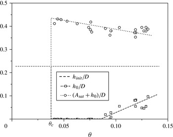
Figure 11. Dimensionless bed thickness versus
 ${\it\theta}$
for
${\it\theta}$
for
 ${\rm\Phi}=0.05$
at the saturated state.
${\rm\Phi}=0.05$
at the saturated state.
Table 1. Results obtained for different protocols for
 ${\rm\Phi}=0.05$
.
${\rm\Phi}=0.05$
.

3.3.1. Geometrical aspect
For
 ${\rm\Phi}=0.05$
and for low flow rates, the erosion on the upstream side is so large that a zone emptied of particles is generated, separating ripples as can be observed in figure 3. The height of the crest,
${\rm\Phi}=0.05$
and for low flow rates, the erosion on the upstream side is so large that a zone emptied of particles is generated, separating ripples as can be observed in figure 3. The height of the crest,
 $h_{0}+A_{sat}$
, and the trough,
$h_{0}+A_{sat}$
, and the trough,
 $h_{0}$
, of bedforms are plotted in figure 11 as a function of the Shields number. It can be seen in this figure that there is an area emptied of particles for
$h_{0}$
, of bedforms are plotted in figure 11 as a function of the Shields number. It can be seen in this figure that there is an area emptied of particles for
 ${\it\theta}<0.08$
. This feature does not appear at higher concentrations (
${\it\theta}<0.08$
. This feature does not appear at higher concentrations (
 ${\rm\Phi}\geqslant 0.1$
), where a minimum bed thickness is observed.
${\rm\Phi}\geqslant 0.1$
), where a minimum bed thickness is observed.
Ouriemi et al. (Reference Ouriemi, Aussillous and Guazzelli2009) also observed this emptied region separating ripples in circular pipes with high-viscosity fluids. They explain it in another way: the erosion of the bed until its complete local extinction is not caused by the action of the main flow, making the particles go away, but by the action of the following vortex, digging and bringing the particles to the new ripple. The fluid viscosity could explain the differences between our observations.
The higher the flow rate, the more the particle flux increases. The erosion phenomenon is amplified with the flow rate, reducing the size of ripples composed of fixed particles. The vortex at the back of each ripple extends, increasing the area of particle deposition. Ripples are thus less steep. Meanwhile, the transport of particles by suspension increases.
Due to the decrease in bed thickness at the crest and the increase in bed thickness at the trough, the ripple amplitude decreases, as illustrated in figure 11. For high flow rates, these features cause the complete extinction of bedforms. An eroded flat bed is thus obtained for flow rates that are too far from the threshold of particle motion. This transition is difficult to determine because the layer of particles in suspension prevent it from being observed.
3.3.2. Wavelength
For each pair of ripples, the length separating the two crests is interpreted as the wavelength. The results of four tests, made at the same flow rate, are reported in figure 12 and show the distribution of this characteristic. The statistical distribution is very close to a normal distribution centred on
 $\overline{{\it\lambda}}_{sat}=20.5~\text{cm}$
with a standard deviation of
$\overline{{\it\lambda}}_{sat}=20.5~\text{cm}$
with a standard deviation of
 ${\it\sigma}\approx 3~\text{cm}$
. This law of distribution was also observed by Kuru et al. (Reference Kuru, Leighton and McCready1995) and Rauen et al. (Reference Rauen, Lin and Falconer2008) but at the wavelet stage. This dispersion has to be kept in mind to remember that, even at the saturated stage when the average characteristics are constant in time and space, ripple characteristics are not perfectly constant.
${\it\sigma}\approx 3~\text{cm}$
. This law of distribution was also observed by Kuru et al. (Reference Kuru, Leighton and McCready1995) and Rauen et al. (Reference Rauen, Lin and Falconer2008) but at the wavelet stage. This dispersion has to be kept in mind to remember that, even at the saturated stage when the average characteristics are constant in time and space, ripple characteristics are not perfectly constant.

Figure 12. Distribution of the length of saturated ripples for
 ${\rm\Phi}=0.05-{\it\theta}\approx 0.13-U_{0}\approx 0.13~\text{m}~\text{s}^{-1}-\mathit{Re}_{0}\approx 3500$
.
${\rm\Phi}=0.05-{\it\theta}\approx 0.13-U_{0}\approx 0.13~\text{m}~\text{s}^{-1}-\mathit{Re}_{0}\approx 3500$
.

Figure 13. Wavelength of saturated ripples and its standard deviation as a function of the Shields number.
The wavelengths measured for all of the tests are averaged and plotted as a function of the Shields number in figure 13. These results show that the wavelength in our experiments can reasonably be considered constant and equal to
 ${\it\lambda}_{sat}=20.3~\text{cm}$
. The fluid velocity seems to have no impact on the saturated wavelength as observed by Raudkivi (Reference Raudkivi1997).
${\it\lambda}_{sat}=20.3~\text{cm}$
. The fluid velocity seems to have no impact on the saturated wavelength as observed by Raudkivi (Reference Raudkivi1997).
3.3.3. Frequency and propagating velocity
While the saturated ripple wavelength does not seem to be influenced by our experimental conditions, this is not the case for the ripple frequency,
 $F_{sat}$
, and the ripple propagating velocity,
$F_{sat}$
, and the ripple propagating velocity,
 $C_{sat}$
, plotted versus the Shields number in figures 14 and 15. An increase in the Shields number induces an increase in both frequency and propagating velocity. This similar evolution of frequency (
$C_{sat}$
, plotted versus the Shields number in figures 14 and 15. An increase in the Shields number induces an increase in both frequency and propagating velocity. This similar evolution of frequency (
 $F_{sat}$
) and propagating velocity (
$F_{sat}$
) and propagating velocity (
 $C_{sat}$
) was expected, as the model of propagating waves states that the propagating velocity is proportional to the frequency and to the wavelength (3.7). Since the wavelength is constant, the propagating velocity evolves in the same way as the frequency:
$C_{sat}$
) was expected, as the model of propagating waves states that the propagating velocity is proportional to the frequency and to the wavelength (3.7). Since the wavelength is constant, the propagating velocity evolves in the same way as the frequency:
 $$\begin{eqnarray}C_{sat}={\it\lambda}_{sat}F_{sat}.\end{eqnarray}$$

Figure 14. Dimensionless frequency of saturated ripples as a function of
 ${\it\theta}$
and
${\it\theta}$
and
 ${\rm\Phi}$
.
${\rm\Phi}$
.

Figure 15. Dimensionless propagating velocity of saturated ripples as a function of
 ${\it\theta}$
and
${\it\theta}$
and
 ${\rm\Phi}$
.
${\rm\Phi}$
.

Figure 16. Evolution of
 $a$
versus
$a$
versus
 ${\rm\Phi}$
.
${\rm\Phi}$
.
The evolution of
 $C_{sat}$
or
$C_{sat}$
or
 $F_{sat}$
, for any solid load, appears linear with the Shields number. The experimental results were therefore fitted using the linear equation system presented in (3.8), where
$F_{sat}$
, for any solid load, appears linear with the Shields number. The experimental results were therefore fitted using the linear equation system presented in (3.8), where
 $a$
and
$a$
and
 $b$
are functions of
$b$
are functions of
 ${\rm\Phi}$
, in order to obtain empirical correlations:
${\rm\Phi}$
, in order to obtain empirical correlations:
 $$\begin{eqnarray}\left\{\!\!\begin{array}{@{}l@{}}\displaystyle \frac{F_{sat}}{\sqrt{g/d}}=a({\it\theta}-{\it\theta}_{c})\\ \displaystyle \frac{C_{sat}}{\sqrt{gd}}=\displaystyle \frac{{\it\lambda}_{sat}}{d}a({\it\theta}-{\it\theta}_{c}).\end{array}\right.\end{eqnarray}$$
This constrained system was fitted. The fitted values
 $a$
and
$a$
and
 ${\it\theta}_{c}$
are reported in figures 14 and 15. The critical value calculated for the Shields number (
${\it\theta}_{c}$
are reported in figures 14 and 15. The critical value calculated for the Shields number (
 ${\it\theta}_{c}=0.034$
) agrees with correlation (3.2).
${\it\theta}_{c}=0.034$
) agrees with correlation (3.2).
Andreotti et al. (Reference Andreotti, Claudin and Pouliquen2006) also observed, for their aeolian sand bedforms, that the propagating velocity is zero at the threshold of motion. However, they found a linear dependency with the shear velocity. This means that bedform velocity is proportional to the square root of the Shields number. Transport by saltation, and not by traction, of sand by air flow could be the cause of this difference.
The parameter
 $a$
, plotted versus
$a$
, plotted versus
 ${\rm\Phi}$
in figure 16, seems to follow a square law, which demonstrates that the Shields number is not sufficient to predict ripple characteristics. A dimensionless parameter, taking into account the geometry of the flow, is necessary and should be identified from more tests.
${\rm\Phi}$
in figure 16, seems to follow a square law, which demonstrates that the Shields number is not sufficient to predict ripple characteristics. A dimensionless parameter, taking into account the geometry of the flow, is necessary and should be identified from more tests.
4. Conclusion
The formation of bedforms with sediment has been studied extensively without being completely elucidated to date. However, the case of bedform generation with particles lighter than the fluid has never been dealt with until now, even though the possibility that stratified floating particles can generate bedforms under continuous flow was first observed by Le Guer et al. (Reference Le Guer, Reghem, Petit and Stutz2003).
The specific design of the facility used for this study enabled bedforms to be generated from a flat bed and maintained in a saturated state. From the observations made, it was possible to identify that the bedforms obtained were vortex ripples. The ripple maturation process was described and the behaviour of the fluid and the solid flow during the saturated state was detailed.
Different methods of analysis were explored to investigate the phenomenon spatially and temporally. These methods, based on Lagrangian and Fourier transforms, were applied to data obtained by image and pressure recording. The results were very close, thus validating the various approaches.
Since the saturated state has been little studied previously, it was important to verify that this state was a stable equilibrium. This was confirmed by checking that the bedforms obtained were independent of the initial conditions and the flow history.
The ripple characteristics during the saturated state were observed as statistically constant over time and space. Nevertheless, the phenomenon was not perfectly regular and a slight dispersion was measured that could be fitted by a normal law. Our results show that, in pipes, the saturated wavelength is not influenced by the flow conditions (cross-section, flow rate). It is likely that either the particle size and/or the pipe size are the key parameters in determining the saturated wavelength. The frequencies and propagation velocities of this kind of bedforms seem to evolve linearly with the Shields number, starting from zero at the threshold of motion and increasing continuously until the gradual disappearance of ripples.
Our set-up enables particle parameters such as density and diameter to be investigated easily, which will be done soon. The influence of the pipe geometry would also be something interesting to explore but would require a complete redesign of the system.
To improve understanding of the phenomenon, a way of determining localised measurements such as velocity profiles and solid fluxes was also studied. However, the small difference in density between the fluid and the particles causes the particles to be in suspension quickly. The layer where the particles move becomes rapidly opaque and investigation by particle image velocimetry or particle tracking velocimetry is not possible. For this kind of mixture the Doppler ultrasound method seems to be the most suitable to investigate local velocity. Knowledge of the mixture’s velocities would help to determine the shear stress at the bed and check different correlations and numerical models.
Acknowledgements
We would like to thank T. Burghelea and P.-C. Czujko for their contributions, discussions and critical analysis of the work done; J. Delmas for technical assistance and H. Joubert for her help in the writing of this paper. This work was undertaken within the framework of the project PERLE 2, funded by the French region Pays de la Loire and monitored by Dr C.C. and Professor T. Brousse.
Appendix A
Peysson et al. (Reference Peysson, Ouriemi, Medale, Aussillous and Guazzelli2009) worked on determining the threshold of motion for sediment particles in a circular pipe. To determine the Shields number, they developed a specific methodology, adapted to this particular case, allowing the evaluation of the wall shear stress at the place where the movement is initiated, i.e. in the middle of the bed. This methodology is valid for any bed heights.
This method is applicable only if the bed is initially flat and not permeable. In our case, the first point is ensure by the protocol used (see figure 10). The second point can be verified by evaluating the Darcy–Forcheimer drag using the Kozeny–Carman equation (Carman Reference Carman1937).
This method consists of determining an equivalent diameter
 $D^{\ast }$
, rather than a hydraulic diameter, depending on the height of the bed, which can be used in the Darcy–Weisbach equation to determine the wall shear stress. This can mathematically be transcribed by (A 1), where
$D^{\ast }$
, rather than a hydraulic diameter, depending on the height of the bed, which can be used in the Darcy–Weisbach equation to determine the wall shear stress. This can mathematically be transcribed by (A 1), where
 ${\it\lambda}$
is the Darcy friction factor, a function depending on a Reynolds number defined in (A 2):
${\it\lambda}$
is the Darcy friction factor, a function depending on a Reynolds number defined in (A 2):
 $$\begin{eqnarray}\displaystyle & \displaystyle {\it\tau}_{b}={\it\lambda}(\mathit{Re}^{\ast })\cdot \frac{{\dot{m}}^{2}}{8{\it\rho}S^{2}} & \displaystyle\end{eqnarray}$$
 $$\begin{eqnarray}\displaystyle & \displaystyle \mathit{Re}^{\ast }=\frac{{\it\rho}D^{\ast }}{{\it\mu}S}. & \displaystyle\end{eqnarray}$$
They propose to use the correlation of Churchill (Reference Churchill1977) to determine
 ${\it\lambda}$
, as this correlation has the advantage of being valid for laminar and turbulent flows.
${\it\lambda}$
, as this correlation has the advantage of being valid for laminar and turbulent flows.
From a large number of numerical resolutions, for laminar flow and different bed heights (denoted
 $h$
), they were able to identify the evolution of the equivalent diameter, given in figure 17. Their result is compared with the hydraulic diameter and shows significant differences.
$h$
), they were able to identify the evolution of the equivalent diameter, given in figure 17. Their result is compared with the hydraulic diameter and shows significant differences.

Figure 17. Evolution of
 $D^{\ast }/D$
and
$D^{\ast }/D$
and
 $D_{h}/D$
depending on
$D_{h}/D$
depending on
 $h/D$
according to Peysson et al. (Reference Peysson, Ouriemi, Medale, Aussillous and Guazzelli2009).
$h/D$
according to Peysson et al. (Reference Peysson, Ouriemi, Medale, Aussillous and Guazzelli2009).


