


1 Introductions
A circular cylinder is one of the simplest geometries, but the flow field around the circular cylinder is complex and changes depending on the Reynolds number ( $Re=\unicode[STIX]{x1D70C}_{\infty }u_{\infty }D/\unicode[STIX]{x1D707}_{\infty }$). Here,
  $\unicode[STIX]{x1D70C}_{\infty },u,_{\infty },D$ and
  $\unicode[STIX]{x1D707}_{\infty }$ are the gas density in the freestream, the freestream velocity, the diameter of the circular cylinder and the dynamic viscosity coefficient in the freestream, respectively. Examination of the flow over a basic shape, such as a flat plate, a circular cylinder or a sphere, is valuable from the viewpoint of understanding the fundamentals of fluid mechanics. Incompressible flows over a circular cylinder have been investigated numerically and experimentally for a wide range of
  $Re$.
$Re$.
Taneda (Reference Taneda1956) conducted a flow visualization experiment and investigated flow structures around a circular cylinder at  $0.1\leqslant Re\leqslant 2000$. He showed that the flow over a circular cylinder is fully attached up to
  $Re$ of 5. The separation occurs at
  $Re=5$, then the length of the recirculation region increases as
  $Re$ increases and becomes an asymmetric recirculation approximately at
  $Re=45$. Dennis & Chang (Reference Dennis and Chang1970) conducted numerical simulations of the wake of a circular cylinder at
  $5\leqslant Re\leqslant 100$ using a finite difference method. Their results showed that the length of the recirculation region approximately linearly increases as
  $Re$ increases. Coutanceau & Bouard (Reference Coutanceau and Bouard1977) visualized the wake of a circular cylinder at
  $5\leqslant Re\leqslant 40$ and showed that the length of the recirculation region increases linearly with increasing
  $Re$. For
  $Re\gtrapprox 47$, the periodic laminar vortex shedding occurs. The effect of
  $Re$ on the Strouhal number (
 $St=fD/u_{\infty }$) of the vortex shedding in the unsteady regime was also studied. Here,
  $f$ is the frequency of the Kármán vortex shedding. Roshko (Reference Roshko1954) measured the vortex shedding frequency of a circular cylinder at
  $40<Re<10\,000$. He showed that
  $St$ of vortex shedding increases as
  $Re$ increases. On the other hand,
  $St$ of vortex shedding is independent of
  $Re$ at
  $300<Re<10\,000$. Roshko (Reference Roshko1961) investigated the flow around a circular cylinder for
  $O(10^{6})<Re<O(10^{7})$ using a pressurized wind tunnel and showed that
  $St$ of vortex shedding was 0.27 at
  $Re>3.5\times 10^{6}$.
Williamson (Reference Williamson1988a,Reference Williamsonb) and Behara & Mittal (Reference Behara and Mittal2010) investigated the three-dimensional effect on  $St$ of vortex shedding and the wake structures. The three-dimensionality in the wake was observed at approximately
  $Re=64$. There is a discontinuity of
  $St$ of vortex shedding in the spanwise direction and a lower frequency was observed in the region near the sidewall. The frequency spectra of the vortex shedding have a single and sharp peak at around
  $64<Re<180$. In this regime, the oblique shedding mode appears and the wake vortices have a slant angle. As
  $Re$ increases, the discontinuity on the
  $Re{-}St$ curve and streamwise vortices appear at around
  $Re=180$. Here, the
  $St$ of vortex shedding discontinuously decreases due to vortex dislocation, and this mode is retained at
  $180<Re<230$ (mode-A). As
  $Re$ further increases, the second discontinuity on the
  $Re{-}St$ curve appears and the
  $St$ of vortex shedding discontinuously increases at approximately
  $Re=230$. In addition, the steady and unsteady aerodynamic force measurements were conducted over a range of
  $Re$ from the onset of two-dimensional oscillations and the conditions that the boundary layer becomes turbulent (Delany & Sorensen Reference Delany and Sorensen1953; Tritton Reference Tritton1959; Gerrard Reference Gerrard1961; Norberg Reference Norberg2001).
The Mach number ( $M=u_{\infty }/a_{\infty }$) affects the flow properties as well as
  $Re$ under compressible flow. Here,
  $a_{\infty }$ is the speed of sound in the freestream. Lindsey (Reference Lindsey1938) was among the first to investigate the effect of
  $Re$ in compressible flow. He measured a drag coefficient (
 $C_{D}$) of a circular cylinder at
  $840\leqslant Re\leqslant 3.1\times 10^{5}$ and
  $0.05\leqslant M\leqslant 0.65$ through wind tunnel tests with an accidental error of
  $\unicode[STIX]{x0394}C_{D}=\pm 2\,\%$, and demonstrated the
  $M$ and
  $Re$ dependences of the drag. Gowen & Perkins (Reference Gowen and Perkins1953) measured the pressure distribution around a circular cylinder in subsonic and supersonic flows and calculated the drag coefficient in the ranges of
  $5.0\times 10^{4}\leqslant Re\leqslant 1.0\times 10^{6}$ and
  $0.3\leqslant M\leqslant 2.9$. They clarified that there is no
  $Re$ effect on the drag coefficient under the supersonic conditions that they investigated. McCarthy & Kubota (Reference McCarthy and Kubota1964) investigated the flow behind a circular cylinder at
  $M=5.7$ and
  $4,500\leqslant Re\leqslant 66\,500$ by measuring the pitot pressure, static pressure and total temperature in the wake with accuracies of
  $\unicode[STIX]{x0394}P/P_{pitot}=\pm 10^{-4}$,
  $\unicode[STIX]{x0394}P/P_{static}=\pm 10^{-3}$ and
  $\unicode[STIX]{x0394}T=\pm 0.5\,^{\circ }\text{F}$, respectively. They determined the transition from laminar to turbulent flow based on the velocity profiles and correlated with the result of mass-diffusion and hot-wire measurements. Murthy & Rose (Reference Murthy and Rose1978) investigated vortex shedding frequencies of a circular cylinder at
  $Re=3.0\times 10^{4}$, 1. 66 × 105 and 5. 0 × 105 for
  $0.25\leqslant M\leqslant 1.2$ by wind tunnel tests. They showed that the
  $St$ of vortex shedding at
  $O(10^{4})\leqslant Re\leqslant O(10^{5})$ is approximately 0.18 for
  $M<0.9$, and there is no detectable vortex shedding at
  $M>0.9$. Rodriguez (Reference Rodriguez1984) investigated the flow over a circular cylinder at
  $1.7\times 10^{5}\leqslant Re\leqslant 3.4\times 10^{5}$ and
  $0.4<M<0.8$. High-speed flow visualizations synchronized with unsteady surface-pressure measurements were conducted, and the relationship between the distribution of the surface pressure and the flow patterns in the near wake were clarified.
Numerical studies have also been conducted by several researchers. Canuto & Taira (Reference Canuto and Taira2015) performed two-dimensional direct numerical simulations (DNS) of compressible flows over a circular cylinder at  $20\leqslant Re\leqslant 100$ and
  $0\leqslant M\leqslant 0.5$. They found that the compressibility effects reduce the growth rate and dominant frequency of the flow instability in the linear growth stage. Xu, Chen & Lu (Reference Xu, Chen and Lu2009) investigated the flow around a circular cylinder at
  $Re=2.0\times 10^{5}$ and
  $0.85\leqslant M\leqslant 0.95$ through detached-eddy simulations (DES). They showed that the flow at
  $M<0.9$ is an unsteady flow characterized by moving shock waves interacting with the turbulent flow in the near region of the circular cylinder, and that the flow at
  $M>0.9$ is a quasi-steady flow with nearly stationary shock waves formed in the near wake. Xia et al. (Reference Xia, Xiao, Shi and Chen2016) computed the compressible flow past a circular cylinder at
  $Re=4.0\times 10^{4}$ and 1. 0 × 106 for
  $0.5\leqslant M\leqslant 0.95$ through constrained large-eddy simulations (CLES). They analysed the effect of
  $M$ on the flow pattern and some statistical quantities such as the drag coefficient and the pressure coefficient distributions. They showed that flow field and flow properties dramatically change around high-subsonic and transonic flows.
Figure 1 shows a map of the condition investigated in the previous studies for compressible flows. Numerical and experimental studies on the compressible flow over a circular cylinder have been conducted at  $O(10^{1})\leqslant Re\leqslant O(10^{2})$ and
  $O(10^{4})\leqslant Re\leqslant O(10^{6})$, respectively. However, few studies examined flows at around
  $Re=O(10^{3})$, and there are no flow visualization studies at this
  $Re$ range. This situation is similar to the case of compressible low-
 $Re$ flows over an isolated sphere. The flow characteristics of the compressible low-
 $Re$ flow over a sphere have been examined by DNS and global stability analysis at
  $Re\leqslant 1000$ (Meliga, Sipp & Chomaz Reference Meliga, Sipp and Chomaz2010; Nagata et al. Reference Nagata, Nonomura, Takahashi, Mizuno and Fukuda2016, Reference Nagata, Nonomura, Takahashi, Mizuno and Fukuda2018a,Reference Nagata, Nonomura, Takahashi, Mizuno and Fukudab,Reference Nagata, Nonomura, Takahashi, Mizuno and Fukudac; Riahi et al. Reference Riahi, Meldi, Favier, Serre and Goncalves2018; Sansica et al. Reference Sansica, Robinet, Alizard and Goncalves2018) and by schlieren visualization through free-flight tests at
  $3.9\times 10^{3}\leqslant Re\leqslant 3.8\times 10^{5}$ (Nagata et al. Reference Nagata, Noguchi, Nonomura, Ohtani and Asai2019). However, there is no report on the unsteady flow properties by computational or visualization studies at
  $Re\approx O(10^{3})$ for compressible flows, because this region is difficult to investigate through either computation or visualization due to the large computational cost or small test model with low-density conditions, respectively.

Figure 1. Map of the conditions investigated in the previous studies. Lindsey (Reference Lindsey1938): exp., drag measurement; Knowler & Pruden (Reference Knowler and Pruden1944): exp., drag and pressure measurement; Gowen & Perkins (Reference Gowen and Perkins1953): exp., drag and pressure measurement, shadowgraph; McCarthy & Kubota (Reference McCarthy and Kubota1964): exp., pitot-pressure, static pressure and total temperature measurements, schlieren; Kitchens & Bush (Reference Kitchens and Bush1972): exp., hot-wire measurement, shadowgraph; Murthy & Rose (Reference Murthy and Rose1977): exp., pressure and skin friction measurement; Dyment & Gryson (Reference Dyment and Gryson1979): exp., shadowgraph and schlieren; Rodriguez (Reference Rodriguez1984): exp., shadowgraph and unsteady pressure measurement; Xu et al. (Reference Xu, Chen and Lu2009): num., DES; Canuto & Taira (Reference Canuto and Taira2015): num., DNS; Xia et al. (Reference Xia, Xiao, Shi and Chen2016): num., CLES.
Knowledge of the compressible low- $Re$ flow is important from the engineering point of view for a high-speed vehicle operated in low-pressure conditions, such as for a Mars exploration aircraft (Hall, Parks & Morris Reference Hall, Parks and Morris1997) or a high-altitude unmanned aircraft (Inokuchi, Tanaka & Ando Reference Inokuchi, Tanaka and Ando2009). It is assumed that these aircraft will be exposed to a compressible low-
 $Re$ flow of
  $O(10^{3})\leqslant Re\leqslant O(10^{5})$. The fundamental knowledge of compressible low-
 $Re$ flow is necessary for the future development of such machines. In addition, investigation of the flow in the condition that has not been investigated is interesting from the point of view of the physics of fluids, and it contributes to extending the knowledge of fluid mechanics. In the present study, we investigated the compressible low-
 $Re$ flows over a circular cylinder at
  $Re=O(10^{3})$ and
  $0.1\leqslant M\leqslant 0.5$ using a low-density wind tunnel and examined the influence of
  $M$ and
  $Re$ on the fundamental characteristics of the flow field, such as flow patterns, the wake structure,
  $St$ of vortex shedding, the pressure coefficient distributions and the drag force coefficient.
2 Methodologies
2.1 Low-density wind tunnel
Figure 2 shows a schematic diagram of the low-density wind tunnel (Anyoji et al. Reference Anyoji, Nose, Ida, Numata, Nagai and Asai2011) used in the present study. The schlieren optical system is also shown in this figure. The low-density wind tunnel consists of an induction-type wind tunnel inside the vacuum chamber and the buffer tank. The vacuum chamber and the buffer tank are connected by a pipe with a butterfly valve. Since a suction-type wind tunnel is installed inside the vacuum chamber, it is possible to change the total pressure of the wind tunnel. In other words,  $M$ and
  $Re$ can be controlled independently. The high-pressure gas is injected from an ejector installed at the downstream of the test section to drive the wind tunnel. A suitable amount of the gas is exhausted to the buffer tank, and the increase of the total pressure in the vacuum chamber is prevented. The amount of the exhausted gas is controlled by a proportion–integration–derivative feedback-controlled butterfly valve. Table 1 shows the specifications of the low-density wind tunnel. The total pressure of the wind tunnel can be set from 1 to 60 kPa. The test duration depends on the total pressure of the wind tunnel, the buffer tank pressure and the ejector supply pressure (typically 2–20 s). The schlieren optical system is described in § 2.3.

Figure 2. Schematic diagram of the low-density wind tunnel and schlieren system.
Table 1. Specifications of the low-density wind tunnel.

2.2 Test model and test condition
Figure 3 shows the test model, which is a circular cylinder of 10 mm diameter. The blockage ratio calculated from the wind tunnel cross-sectional area and the frontal area of the test model was approximately 6 %. Four test models were used, which are test models for schlieren visualization (figure 3a), force and pressure measurements (figure 3b), unsteady pressure measurements using an unsteady pressure sensor (figure 3c) and unsteady pressure measurements using anodized-aluminum pressure-sensitive paint (AA-PSP) (Sakaue Reference Sakaue1999) (figure 3d). Part of the sidewalls of the test section was replaced by optical glasses when conducting the schlieren visualization, and the test model was mounted on the optical glass, as shown in figure 3(e). The spanwise length of the test model for schlieren visualization and unsteady pressure measurements was 100 mm. The test model for the steady pressure and force measurements was 99.7 mm in order to avoid interference with the sidewall in the force measurement. The model for steady pressure measurements has three pressure taps of a diameter in 0.1 mm, and the model for unsteady pressure measurements has one pressure tap of a diameter in 0.5 mm. The unsteady pressure sensor was installed in the model.
Table 2 shows the test condition. The total pressure of the wind tunnel was less than or equal to 20 kPa in order to realize the compressible low- $Re$ flow. However, the flow visualization by the schlieren method is difficult under the low-density condition (i.e. low-
 $Re$ conditions) because the density fluctuation becomes weak.

Figure 3. Test modes: (a) for schlieren visualization; (b) for steady pressure measurement; (c) for unsteady pressure measurement; (d) for PSP measurement (e) mounted model on the optical window (schlieren set-up).
Table 2. Experimental conditions.

2.3 Schlieren visualization
Flow visualization was carried out with optical windows (diameter: 95 mm) on the sidewall of the wind tunnel. A light-emitting-diode light (LET Q9 WP, Osram), which has a peak emission wavelength of 530 nm, was used as a light source. The light beam from the light source was collimated by a plano-convex lens with a focal length of 1000 mm, and the parallel light beam was converged with the same plano-convex lens. Forty per cent of the light flux was horizontally cut by a knife edge. The imaging lens was a convex lens with a focal length of 250 mm. A high-speed camera (Fastcam SA-X2, Photron) was used to take time-series schlieren images. The image resolution was 768 × 384 pixel, and the frame rate was 20 000 fps with an exposure time of 47.2 μs.
Figure 4 shows the image processing procedure. Time averaging and fast Fourier transform (FFT) were applied, and the flow geometry and  $St$ of vortex shedding were investigated. In addition, background image subtraction was carried out on the time-series images to reduce the pattern, which is not related to flow phenomena. Here,
  $St$ of vortex shedding was computed by the FFT analysis for each pixel of the time-series images, and the frequency that has the largest power spectral density (PSD) was selected as the primary peak frequency of the vortex shedding. Here, the frequency spectra were evaluated as the averaged value in the whole of the schlieren image. The frequency resolution of the FFT in the present study was 9.7 Hz in all cases. In addition, the characteristic length of the flow field was measured on the time-averaged images.

Figure 4. Flowchart of the image processing.

Figure 5. Schematic diagram of the set-up for the AA-PSP measurement.
2.4 Force and pressure measurements
Steady force and pressure measurements were performed at the same time. A balance system using the load cells (LC-4101-G-600; A&D) was used for the steady force measurement. The range and accuracy of the load cell for the drag measurement were 6 N and 0. 9 × 10⁻³ N, respectively. The output signal from the load cell was amplified by a direct-current strain amplifier (DSA-100A; Nissho Electricworks). In addition, steady and unsteady pressure measurements were conducted. The model for the steady pressure measurement has three pressure taps, which are connected to a pressure scanner (NetScanner System 9116; Pressure Systems, Inc.). Pressure data for circumferential angles from 0 to 180° were acquired every 6° by rotating the test model. The model for unsteady pressure measurement has one pressure tap, which is connected to an unsteady pressure sensor installed in the model (CCQ-093-5A, Kulite Semiconductor Products Inc.). The signal from the unsteady pressure sensor was amplified by an amplifier (570ST, TEAC) and filtered by an analogue low-pass filter (2625, NF Corporation). The signals were recorded by a data logger (WE7000, Yokogawa) with a sampling frequency of 50 000 Hz. In addition, AA-PSP was used for time-resolved visualization of the pressure fluctuation on the cylinder surface. Figure 5 shows the schematic diagram of the experimental set-up of the PSP measurement. Two blue-LEDs (IL-106, Hardsoft) and a high-speed camera (Fastcam SA-X2, Photron) were used as an excitation light of the AA-PSP and for imaging, respectively. A camera lens (Nikkor 135 mm f/2.0, Nikon) was used as an imaging lens with a long-pass filter (590 nm) to cut off the light other than the emission of the AA-PSP. The pressure and temperature sensitivities of the AA-PSP that was used in the present study were approximately 6 %/kPa and 0.9 %/K, respectively, in atmospheric pressure of 1–10 kPa at a temperature of 278–293 K. A flowchart of the image processing for the AA-PSP measurements is shown in figure 6. In the present study, the objective of AA-PSP measurements was a visualization of the phase difference of the Kármán vortex shedding in the spanwise direction, so that only the pressure fluctuation from the time- and space-averaged pressure on the cylinder surface ( $\unicode[STIX]{x0394}C_{p}$) was computed, and the PSD and phase images were processed. In addition, the randomized singular value decomposition (rSVD) proposed by Feng et al. (Reference Feng, Xie, Song, Yu and Tang2018) was applied to the time-series images of the
  $\unicode[STIX]{x0394}C_{p}$, and the noisy modes (higher modes) were discarded to reduce the noise. In the present study, the number of power procedures was one time, and the most energetic 200 modes were used to reconstruct the PSP images.

Figure 6. Flowchart of the image processing of the AA-PSP measurement.
3 Instantaneous flow field
3.1 Wake structure
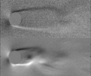
Figures 7 and 8 show the influence of  $Re$ at
  $M=0.5$ and the influence of
  $M$ at
  $Re=1000$, respectively, on the instantaneous flow structure. The separated shear layers are generated at the separation point on the cylinder, and the recirculation region and the Kármán vortex street are formed downstream of the cylinder. Figure 7 illustrates that the release location of the Kármán vortices moves upstream as
  $Re$ increases because the instability of the separated shear layer becomes strong with increasing
  $Re$ similar to the incompressible cases. It should be noted that the signal-to-noise ratio of the schlieren images decreases as
  $Re$ decreases due to a decrease in the atmospheric density, because the absolute value of the density fluctuation becomes small, and hence the density gradient becomes small.

Figure 7. Effect of  $Re$ on the instantaneous flow field at
  $M=0.5$. (a)
  $Re=1000$; (b)
  $Re=2000$; (c)
  $Re=3000$; (d)
  $Re=4000$.

Figure 8. Effect of  $M$ on the instantaneous flow field at
  $Re=1000$. (a)
  $M=0.2$; (b)
  $M=0.3$; (c)
  $M=0.4$; (d)
  $M=0.5$.
Figure 8 shows the  $M$ effect on the instantaneous flow structure at
  $Re=1000$. The generation of the separated shear layer and the formation of the Kármán vortices can be seen. Also, the length of the separated shear layer seems to be extended as
  $M$ increases. However, the schlieren image acquired by the present study is unclear, particularly at lower-
 $M$ and low-
 $Re$ conditions due to the small density fluctuation. Therefore, root-mean-square (r.m.s.) of the intensity of schlieren images was computed, and the distance between the downstream stagnation point of the cylinder and the maximum r.m.s. position
  $L_{rms\_max}$ was explored. In the present study, it was assumed that the maximum r.m.s. point is related to the pinch-off location of the Kármán vortices and the end of the recirculation region. The length of the recirculation region at
  $Re=20$ and 40 monotonically increase as
  $M$ increases for
  $0.1\leqslant M\leqslant 0.5$ (Canuto & Taira Reference Canuto and Taira2015). However, figure 9 illustrates that the
  $M$ dependence on
  $L_{rms\_max}$ is different between
  $Re\leqslant 3000$ and
  $Re\geqslant 4000$. In addition, there is an inflection point in the
  $M$ evolution on
  $L_{rms\_max}$ at
  $Re=2000$ and 3000, respectively. Hence, there is a difference in the influence of the
  $M$ effect on
  $L_{rms\_max}$ at
  $Re=O(10^{1})$ and
  $Re=O(10^{3})$. At
  $Re=3000$,
  $L_{rms\_max}$ decreases as
  $M$ increases up to
  $M=0.3$ and increases for
  $0.3\leqslant M\leqslant 0.5$. The separated shear layer is stabilized as
  $M$ increases because the Kelvin–Helmholtz instability is suppressed due to the compressibility effect, and thus the length of the recirculation region increases as
  $M$ increases. The increase in the length of the recirculation region with increasing
  $M$ has also been reported by Canuto & Taira (Reference Canuto and Taira2015) at
  $Re\leqslant 40$. The trend on
  $L_{rms\_max}$ at
  $Re=2000$ is similar to that at
  $Re=3000$, but the decrement and increment of
  $L_{rms\_max}$ are smaller than at
  $Re=3000$. For
  $Re\geqslant 4000$, on the other hand,
  $L_{rms\_max}$ monotonically decreases as
  $M$ increases, hence
  $L_{rms\_max}$ moves upstream as
  $M$ increases. The reason why
  $L_{rms\_max}$ decreases as
  $M$ increases at
  $M\geqslant 0.3$ for
  $Re\geqslant 4000$ seems to be the influence of the oblique instability wave on the separated shear layer due to the compressibility effect. The oblique instability wave is suppressed due to viscous and compressibility effects at lower-
 $Re$ conditions. Conversely, the oblique instability surpasses the stabilization effect due to compressibility effects as
  $Re$ increases because of the decrease of the stability for higher-
 $Re$ conditions. Hence, the
  $M$ effect on
  $L_{rms\_max}$ at
  $M\geqslant 0.3$ seems to be different for
  $Re\leqslant 3000$ and
  $Re\geqslant 4000$. The detailed discussions of the oblique instability, which connects to the spanwise flow structure, appear in § 3.2.

Figure 9. Effect of  $M$ on the position of the maximum r.m.s. of intensity of the schlieren image.
3.2 Planar distribution of pressure fluctuation
Figure 10 shows the results of AA-PSP measurements at  $2000\leqslant Re\leqslant 5000$ and
  $M\geqslant 0.3$. The left-hand side of figure 10 shows the PSD distribution of the pressure coefficient fluctuation (
 $\unicode[STIX]{x0394}C_{p}$) at the frequency of the Kármán vortex shedding. The distribution of PSD illustrates that the pressure fluctuation on the cylinder surface becomes stronger as
  $M$ increases. The right-hand side of figure 10 shows the phase difference of the pressure fluctuation from the reference point, which is located in the centre of the cylinder on the PSP images. There is no phase difference in the spanwise direction at
  $Re=2000$ for
  $M\leqslant 0.5$, at
  $Re=3000$ for
  $M\leqslant 0.4$, at
  $Re=4000$ for
  $M\leqslant 0.4$ or at
  $Re=5000$ for
  $M\leqslant 0.3$. However, this figure also shows that the phase difference in the spanwise direction can be observed at
  $Re=3000$ and 4000 at
  $M=0.5$ and
  $Re=5000$ at
  $M=0.4$, respectively. Therefore, the spanwise phase difference appears at higher-
 $Re$ and -
 $M$ conditions in the conditions investigated in the present study. Also, the phase difference in the spanwise direction at
  $Re=4000$ and
  $M=0.5$ is larger than that at
  $Re=5000$ and
  $M=0.4$ so that the
  $M$ effect seems to be more important than the
  $Re$ effect on the phase difference.
The phase difference in the pressure fluctuation is considered to be due to the oblique instability wave in the separated shear layer. The large-scale spanwise-aligned vortices, i.e. the Brown–Roshko vortices, are the dominant structures in the parallel shear layer under incompressible flow (Brown & Roshko Reference Brown and Roshko1974). The convective Mach number ( $M_{c}=(U_{1}-U_{2})/(a_{1}+a_{2})$) introduced by Bogdanoff (Reference Bogdanoff1983) is important to discuss the shear layer in the compressible flow. Here, subscripts 1 and 2 indicate the high-speed and low-speed sides, respectively, in the shear layer. Bogdanoff (Reference Bogdanoff1983) and Papamoschou & Roshko (Reference Papamoschou and Roshko1988) showed that the growth rate of the turbulent shear layer due to the compressibility effect appears approximately above
  $M_{c}=0.3$. In addition, Sandham & Reynolds (Reference Sandham and Reynolds1990, Reference Sandham and Reynolds1991) conducted DNS of the compressible Navier–Stokes equations. They showed that a three-dimensional structure called the
  $\unicode[STIX]{x1D6EC}$-vortex appears at
  $M_{c}>0.6$, and its growth rate surpasses that of the two-dimensional structure.

Figure 10. Distributions of PSD and phase difference of  $\unicode[STIX]{x0394}C_{p}$. (a)
  $Re=2000$; (b)
  $Re=3000$; (c)
  $Re=4000$; (d)
  $Re=5000$. The reference point is the centre of the cylinder surface in the spanwise direction.
The maximum fluid velocity around the cylinder in potential flow is double the freestream velocity. Therefore,  $M_{c}$ appears to be close to 0.6 in the case of
  $M=0.5$. The separated shear layers released from the cylinder are the shear layers between the flow in the recirculation region and its outer flow, and thus the flow physics of the separated shear layer seems to be similar. Hence, the oblique instability caused by the compressibility effects appears to occur, and it causes the spanwise phase differences in the pressure fluctuation. A smaller phase difference is thought to have occurred at
  $M=0.5$ and
  $Re<3000$, as compared to
  $M=0.5$ and
  $Re=5000$ because the growth of the oblique instability wave is reduced by a decrease in
  $Re$. In such a case, it is considered that the phase difference in the vortex shedding appears further downstream.
There is another possibility of the phase difference in the spanwise direction that has been observed in incompressible flows. The frequency discontinuity on the vortex shedding appears in the spanwise direction at  $Re<64$. In addition, the oblique shedding (
 $64<Re<180$), mode-A (
 $180<Re<230$) and mode-B (
 $Re>230$) appear at lower-
 $Re$ conditions of the incompressible flows. The slant angle of the wake was observed and its angle was approximately 10°–20° in the oblique shedding regime (Williamson Reference Williamson1988a,Reference Williamsonb). However, the
  $Re$ range investigated in the present study is
  $Re=O(10^{3})$, and thus the wake is at least mode-B or a more complicated structure and is fully three-dimensional. In the present study, visualization of the wake structure in the spanwise direction could not be conducted due to the structure of the experimental equipment so that the slant angle was estimated from the phase difference in the surface pressure fluctuation, the primary vortex shedding frequency and the estimated convective velocity of the separated shear layer. As a result, the estimated slant angle was less than 6° for all cases for which a phase difference was observed. It is estimated that the slant angle that was observed in the present study should be quite small because the angle of the oblique instability wave
  $\unicode[STIX]{x1D719}$ due to the compressibility effect is dominated by
  $M_{c}$ and can be estimated by the following equation (Sandham & Reynolds Reference Sandham and Reynolds1990):
 $$\begin{eqnarray}M_{c}\cos \unicode[STIX]{x1D703}\approx 0.6.\end{eqnarray}$$
 The flow conditions investigated in the present study seem to be close to the critical condition for the oblique instability so that the oblique instability wave is weak even though it appears. The small slant angle in the wake also appears in incompressible flows at  $Re<64$. In this flow pattern, another peak, ‘competing frequency’ (see Williamson Reference Williamson1988a), near the primary vortex shedding frequency appears so that the characteristics of the frequency spectra are changed by the three-dimensionality of the wake. In this case, the frequency of the vortex shedding is slightly changed in the spanwise direction. The higher frequency corresponds to the vortex shedding frequency in the centre region of the cylinder in the spanwise direction. The lower frequency corresponds to the vortex shedding frequency in the region near the sidewall. However, there are no such peaks in the present study except for
  $M=0.5$ at
  $Re=4000$. Therefore, ‘competing frequency’ is at least not related to the spanwise phase difference due to the
  $M$ effect.
Figure 11 shows the frequency spectra of the pressure fluctuation. The time-resolved pressure data were acquired by the unsteady pressure sensor at  $\unicode[STIX]{x1D703}=70^{\circ }$ and the FFT analysis was conducted. Here,
  $\unicode[STIX]{x1D703}$ indicates the angle from the upstream stagnation point. The frequency spectra have two peaks at approximately
  $St=0.2$ and 0.4 for each condition. The first peak is the frequency of the Kármán vortex shedding and the second one is its second harmonic wave. There is no large influence of
  $Re$ on the peak frequency at
  $M\leqslant 0.3$. Conversely, the peak frequency increases as
  $Re$ increases at
  $M>0.3$, particularly at
  $Re\geqslant 4000$, and the peak develops a blunt shape as
  $M$ increases. In addition, another peak appears near the primary peak at
  $Re=4000$ and
  $M=0.5$. The shift of peak seems to be caused by the oblique instability wave due to the compressibility effect. The effect of
  $M$ on the
  $St$ of vortex shedding is weak in low-
 $M$ cases. For higher-
 $M$ cases, on the other hand, the
  $St$ of vortex shedding decreases and increases as
  $M$ increases at
  $Re\leqslant 3000$ and
  $Re\geqslant 4000$, respectively. The separated shear layer is stabilized by the compressibility effect, and
  $St$ of vortex shedding decreases at
  $Re\leqslant 3000$. A similar trend was observed for the sphere at
  $Re\leqslant 1000$ (Nagata et al. Reference Nagata, Nonomura, Takahashi, Mizuno and Fukuda2016, Nagata et al. Reference Nagata, Nonomura, Takahashi and Fukudaunder review). Conversely, at
  $Re\geqslant 4000$, the oblique instability wave appears, and
  $St$ of vortex shedding increases. The oblique instability is not considered to appear at
  $Re\leqslant 3000$ because of the stronger viscous effect. Hence, the slight changes in the peak frequency and peak shape of the frequency spectra seem to be related to the oblique instability wave caused by compressibility effects. However, further investigations using numerical methods such as global stability analysis are essential to clarify the details of flow physics.

Figure 11. Distributions of PSD and phase difference. (a)  $M=0.2$; (b)
  $M=0.3$; (c)
  $M=0.4$; (d)
  $M=0.5$. The reference point is the centre of the cylinder surface in the spanwise direction.

Figure 12. Effect of  $Re$ on
  $St$ of vortex shedding.

Figure 13. Effect of  $M$ on
  $St$ of vortex shedding.
3.3 Strouhal number of vortex shedding
Figure 12 illustrates the influence of  $Re$ on
  $St$ of vortex shedding. Here,
  $St$ of vortex shedding is estimated based on the time-series schlieren images through the FFT analysis. The results show that
  $St$ of vortex shedding increases as
  $Re$ increases and its increment becomes large as
  $M$ increases. The effect of
  $Re$ on
  $St$ of vortex shedding is similar in each
  $M$ case. In addition, figure 13 shows the influence of
  $M$ on
  $St$ of vortex shedding. The
  $St$ of vortex shedding is not related to
  $M$ at
  $M\leqslant 0.3$, but
  $St$ of vortex shedding increases and decreases as
  $M$ increases for
  $Re\leqslant 3000$ and
  $Re\geqslant 4000$, respectively, at
  $M>0.3$. The trend at
  $Re\leqslant 3000$ is similar in the flows over a circular cylinder and over a sphere for lower-
 $Re$ conditions of
  $O(10^{1})\leqslant Re\leqslant O(10^{2})$ (Canuto & Taira Reference Canuto and Taira2015; Nagata et al. Reference Nagata, Nonomura, Takahashi, Mizuno and Fukuda2016), because a part of the fluctuation energy of the fluid is consumed for the expansion and compression of the fluid due to aeroelasticity. At
  $Re\geqslant 4000$, however,
  $St$ of vortex shedding increases as
  $M$ increases. Hence, the trend of the
  $M$ dependence on
  $St$ of vortex shedding is different in
  $Re\leqslant 3000$ and
  $Re\geqslant 4000$. According to the results of the AA-PSP measurement shown in figure 10, the phase difference of the vortex shedding in the spanwise direction becomes large as
  $Re$ increases at
  $Re\geqslant 4000$ so that the change of the
  $M$ effect on
  $St$ of vortex shedding might be related to the oblique instability caused by the compressibility effect. In the case of the incompressible low-
 $Re$ flow, the vortex shedding frequency discontinuously decreases and increases due to the mode transition from oblique shedding to mode-A at
  $Re\approx 180$ and from mode-A to mode-B at
  $Re\approx 230$, respectively. The Strouhal number of the vortex shedding discontinuously decreases in the case of the transition to mode-A. In this case, streamwise vortices are generated due to vortex dislocation, and the vortices appear every 3–4
 $D$ in the spanwise direction. In the case of the transition to mode-B, on the other hand,
  $St$ of the vortex shedding discontinuously increases, and the interval between streamwise vortices becomes approximately 1
 $D$. Therefore, from the viewpoint of
  $St$ of the vortex shedding, the mode transition due to compressibility effects observed in the present study is similar to the transition from the mode-A to mode-B in incompressible flow. However, in the conditions investigated in the present study was quite higher
  $Re$ so that the phase difference observed by PSP measurement is considered to be not related to the three-dimensional instability observed in the previous incompressible lower-
 $Re$ flows. Instead of that, it is considered that is due to the oblique instability in the shear layer by the compressibility effect discussed in figure 10. The increase in
  $St$ of vortex shedding reflects the destabilizing effect of the recirculation region. The phenomena that support this trend appear in
  $L_{rms\_max}$ discussed in figure 9.

Figure 14. Effect of  $Re$ on the time-averaged flow field at
  $M=0.5$. (a)
  $Re=1000$; (b)
  $Re=2000$; (c)
  $Re=3000$; (d)
  $Re=4000$.
4 Time-averaged flow fields
4.1 Mean-flow structure
Figures 14 and 15 show the  $Re$ and
  $M$ effects on the time-averaged flow field. The separated shear layers released from the cylinder surface are clearly visualized in the time-averaged images. The clearance between the upper and lower sides of the separated shear layer gradually increases downstream, and the separated shear layer becomes unclear in the vicinity of the pinch-off location of the Kármán vortices. Also, strong density fluctuations appear in the region where the Kármán vortices are released, while the time-averaged schlieren pattern forms a closed structure that looks like the recirculation region. Note that the schlieren pattern around the end of the recirculation region is weak for the case of the low-dynamic-pressure condition. Figure 14 illustrates that the clear region of the separated shear layers becomes short so that the recirculation region becomes small as
  $Re$ increases due to lower stability of the separated shear layer. Figure 15 illustrates that the influences of
  $M$ on the time-averaged flow field, on the other hand, do not clearly appear at
  $Re=1000$ in subsonic flows due to the low-density conditions. The maximum width of the separated shear layer
  $W_{max}$ was measured on the time-averaged images by tracking high- and low-intensity locations and the flow structure is characterized hereinafter.

Figure 15. Effect of  $M$ on the time-averaged flow field at
  $Re=1000$. (a)
  $M=0.2$; (b)
  $M=0.3$; (c)
  $M=0.4$; (d)
  $M=0.5$.

Figure 16. Effect of  $Re$ on the maximum width of the separated shear layer.
Figures 16 and 17 show the relationships between  $W_{max}$ and
  $Re$ and between
  $W_{max}$ and
  $M$, respectively. Figure 16 illustrates that
  $W_{max}$ decreases as
  $Re$ increases, and the trend is the same in each
  $M$. Here, the trajectory of the separated shear layer is similar in all of the conditions investigated in the present study so that
  $W_{max}$ is considered to be strongly related to the length of the recirculation region. Therefore, the length of the recirculation region is inferred to decrease as
  $Re$ increases. This trend is also observed in figure 7 and is similar to that under incompressible flow conditions for the same
  $Re$ range. Based on figure 17,
  $W_{max}$ increases as
  $M$ increases for
  $Re\leqslant 3000$. This implies that the length of the recirculation region increases as
  $M$ increases for
  $Re\leqslant 3000$, and the trend is similar to those in previous studies for lower-
 $Re$ conditions of
  $O(10^{1})\leqslant Re\leqslant O(10^{2})$ and
  $O(10^{2})\leqslant Re\leqslant O(10^{3})$ of the flows over a cylinder (Canuto & Taira Reference Canuto and Taira2015) and over a sphere (Nagata et al. Reference Nagata, Nonomura, Takahashi, Mizuno and Fukuda2018b), respectively. Conversely,
  $W_{max}$ decreases as
  $M$ increases for
  $Re\geqslant 4000$, so that the influence of
  $M$ on
  $W_{max}$ changes at
  $Re$ ranging from 3000 and 4000. The results of AA-PSP measurements discussed in § 3.2 show the possibility that the above change is owing to the spanwise phase difference of the vortex shedding due to the oblique instability wave.

Figure 17. Effect of  $M$ on the maximum width of the separated shear layer.
4.2 Distribution of pressure coefficient
Figure 18 shows the  $M$ effect on the distribution of the time-averaged pressure coefficient in the streamwise direction at the centre of the cylinder in the spanwise direction. The horizontal axis, which shows
  $\unicode[STIX]{x1D703}$, indicates the angle from the upstream stagnation point. Figure 18 illustrates that
  $C_{p}$ at the upstream stagnation point increases slightly as
  $M$ increases and agrees well with isentropic theory, as shown in figure 19, because the viscous effects near the upstream stagnation point is minimal because of the thin boundary layer. Here, the standard deviation of the measured pressure at the upstream stagnation point was 0.004–0.03, and the error on the stagnation pressure based on the standard deviation was less than 2.6 % of the measured pressure. The trend of the
  $M$ effect on the time-averaged pressure coefficient reverses around
  $\unicode[STIX]{x1D703}=45^{\circ }$ so that
  $C_{p}$ decreases as
  $M$ increases for
  $\unicode[STIX]{x1D703}>45$. This kind of result can be expected from the Prandtl–Glauert transformation (Glauert Reference Glauert1928). The compressibility effect described by the Prandtl–Glauert transformation works to increase the absolute value of
  $C_{p}$ in the attached region, and thus
  $C_{p}$ becomes higher and lower as
  $M$ increases in the region where
  $C_{p}>0$ and
  $C_{p}<0$, respectively. A similar trend can be observed at lower- and higher-
 $Re$ conditions. The reverse of
  $M$ effect on the
  $C_{p}$ distribution appears at around
  $\unicode[STIX]{x1D703}=90^{\circ }$ in the case of lower-
 $Re$ conditions of
  $Re=20$ and 40 (Canuto & Taira Reference Canuto and Taira2015). Also, the same phenomenon was observed at around
  $\unicode[STIX]{x1D703}=60^{\circ }$ at higher
  $Re$ of
  $Re=166\,000$ by Murthy & Rose (Reference Murthy and Rose1977) (see Zdravkovich (Reference Zdravkovich1997), p. 503). The position of the reverse of
  $C_{p}$ seems to be related to the position of the separation point. The reverse of
  $M$ effect on
  $C_{p}$ distribution does not appear at the further high
  $Re$ of
  $500\,000$. In this
  $Re$ range, the absolute value of
  $C_{p}$ for the low-subsonic condition is larger due to the turbulent transition. At higher-
 $M$ conditions, on the other hand, the absolute value of
  $C_{p}$ is smaller than that of incompressible flows due to suppression of the turbulence transition caused by the compressibility effect, so that reverse of the
  $M$ effect on
  $C_{p}$ distribution is not observed in this
  $Re$ range.

Figure 18. Time-averaged pressure coefficient distribution for different  $M$ (
$M$ ( $Re=4000$).

Figure 19. Measured and theoretical values of the pressure coefficient at the upstream stagnation point.
Figure 20 shows the influence of  $M$ on the minimum
  $C_{p}$ location
  $\unicode[STIX]{x1D703}_{C_{p}min}$ for different
  $Re$ conditions. A previous incompressible study by Takada (Reference Takada1975) reported that
  $\unicode[STIX]{x1D703}_{C_{p}min}$ is related to the position of the separation point because the separation point is located between the minimum
  $C_{p}$ location and the pressure recovery region, and the position of the separation point can be estimated by the position of
  $\unicode[STIX]{x1D703}_{C_{p}min}$. In the present study, the
  $C_{p}$ distribution was measured discretely, thus,
  $\unicode[STIX]{x1D703}_{C_{p}min}$ was estimated by the fitted curve of the
  $C_{p}$ distribution at around
  $\unicode[STIX]{x1D703}=70^{\circ }$. Figure 18 illustrates that the location of
  $\unicode[STIX]{x1D703}_{C_{p}min}$ tends to move downstream as
  $M$ increases. Therefore, the position of the separation point appears to move downstream as
  $M$ increases. This trend agrees with the
  $M$ effect on the viscous drag coefficient, which will be discussed in figure 21. On the other hand, the
  $M$ effect on
  $\unicode[STIX]{x1D703}_{C_{p}min}$ is quite small at
  $Re=20$ and 40 (Canuto & Taira Reference Canuto and Taira2015). Their results indicate that the position of the separation point is approximately constant even though
  $\unicode[STIX]{x1D703}_{C_{p}min}$ moves downstream as
  $M$ increases, the change in the position of the separation point from
  $M=0$ to 0.5 is less than 0. 5°. Therefore, there is the difference in the effect of
  $M$ on the position of the separation point at
  $Re=O(10^{1})$ and
  $O(10^{3})$.

Figure 20. Effect of  $M$ on the position of
  $\unicode[STIX]{x1D703}_{C_{p},min}$.

Figure 21. Effect  $M$ on the drag coefficient. (a) Total; (b) pressure component; (c) viscous component (Lindsey Reference Lindsey1938).
4.3 Drag coefficient
Figure 21 shows the  $M$ effect on the total, pressure and viscous drag coefficients. In the present study, the total drag coefficient was measured by a balance system. The pressure drag was calculated from the pressure distribution acquired by the steady pressure measurement, and the viscous drag was calculated by subtracting the pressure drag from the total drag. The standard deviation of the drag coefficient was approximately 0.02–0.04. The error on the drag coefficient based on the standard deviation was less than 3.4 % of the total drag coefficient and the percentage of the error based on the standard deviation increases as
  $Re$ and
  $M$ decrease. Figure 21(a) illustrates that the total drag coefficient increases as
  $M$ increases for each
  $Re$ condition, and figure 21(b) shows that the increment of the total drag coefficient is almost due to the increment of the pressure component, because the compressibility effect, which can be explained by the Prandtl–Glauert transformation, is dominant on the increment of the pressure drag in this
  $Re$ range. This trend is similar to that of the previous study at the lower-
 $Re$ condition (Canuto & Taira Reference Canuto and Taira2015). Figure 21(c) illustrates that the viscous component of the drag coefficient increases as
  $M$ increases but the increment is quite small. The increment of the viscous drag coefficient due to compressibility effects increases as
  $Re$ decreases because the estimated position of the separation point by
  $\unicode[STIX]{x1D703}_{C_{p}min}$ appears to move downstream as
  $M$ increases and the effect of viscosity becomes more effective as
  $Re$ decreases. In addition, the amount of movement of the separation point due to compressibility effects increases as
  $Re$ decreases, and thus, the increment of the viscous drag coefficient appears to reflect the movement of the position of the separation point.

Figure 22. Relationship between  $W_{max}/D$ and
  $St$ of vortex shedding.
5 Characterization of flow properties by flow geometry
5.1 Characterization of Strouhal number of vortex shedding
Figure 22 shows the relationship between  $W_{max}/D$ and
  $St$ of vortex shedding. As discussed in § 3.3,
  $St$ of vortex shedding depends on
  $Re$ and
  $M$ so that
  $St$ does not monotonically decrease with respect to
  $M$ (symbols in figure 22 are connected by solid lines in order of
  $M$ for each
  $Re$). However,
  $St$ of vortex shedding can be characterized by
  $W_{max}/D$ approximately regardless of the freestream condition. Figure 22 illustrates that the
  $St$ of vortex shedding tends to be small when
  $W_{max}/D$ is large. Here,
  $W_{max}/D$ on the time-averaged field appears to reflect the length of the recirculation region because the separation angle is almost the same in all the cases, thus, the length of the recirculation region is large when
  $W_{max}/D$ is large. In other words, the size of the recirculation region is large when
  $W_{max}/D$ is large. If the recirculation region is unstable, the size of the recirculation region in the time-averaged field is small and
  $St$ of vortex shedding is large. The effect of
  $M$ also seems to appear because the development speed of the vortices in the recirculation region is different due to compressibility effects, and its effect also can be characterized by
  $W_{max}/D$. Figure 23 shows the relationship between
  $Re$ and
  $St_{W_{max}}$, which is the
  $St$ of vortex shedding based on the freestream velocity and
  $W_{max}/D$. The parameter
  $St_{Wmax}$ also gives good characterization since the frequency of the vortex shedding is strongly influenced by the size of the recirculation region, as discussed with figure 22. In addition, the development speed of vortices in the recirculation region depends on
  $Re$, so that
  $St$ of vortex shedding can be characterized by
  $W_{max}/D$ and
  $Re$.
$Re$.

Figure 23. Relationship between  $Re$ and
  $St$ of vortex shedding based on
  $W_{max}/D$.
5.2 Characterization of drag coefficient
Figure 24 shows the relationship between  $W_{max}/D$ and the drag coefficient
  $C_{d}$. In incompressible flows, the size of the recirculation region is related to the pressure drag because the pressure drag is determined by the backpressure, and then the size of the recirculation region is related to the backpressure. Also, as shown in figure 21, the change in the viscous drag coefficient due to the
  $Re$ effect is quite a bit smaller than that in the pressure drag coefficient, and thus the total drag coefficient appears to be characterized by the size of the recirculation region if there are no compressibility effects. Figure 24(a) shows the relationship between
  $W_{max}/D$ and the drag coefficient. As shown in figure 24(a), the drag coefficient can be characterized by
  $W_{max}/D$, the drag coefficient decreases as
  $W_{max}/D$ increases. However, there is the strong compressibility effect on the
  $W_{max}/D{-}C_{d}$ curve. In figure 24(b), the vertical axis is
  $C_{d,PG}$ which corresponds to the corrected drag coefficient by the Prandtl–Glauert transformation as follows:
 $$\begin{eqnarray}C_{d,PG}=C_{d}\sqrt{1-M^{2}}.\end{eqnarray}$$
 Here,  $C_{d}$ is the measured drag coefficient that includes the compressibility effect,
  $C_{d,PG}$ is the corrected drag coefficient which is the drag coefficient excluding the compressibility effect estimated using the Prandtl–Glauert transformation. In the condition investigated in the present study,
  $M$ effects on the viscous drag are sufficiently smaller than that on the pressure drag as discussed in § 4.3. Hence, the Prandtl–Glauert transformation was applied to the total drag coefficient. Figure 24(b) illustrates that the effect of
  $M$ on the
  $W_{max}/D{-}C_{d}$ curve is reduced, and thus a better characterization can be obtained. This means that the
  $M$ effect on
  $C_{d}$ can approximately be characterized by the compressibility effect, which is described by the Prandtl–Glauert transformation. In particular,
  $C_{d,PG}$ depends only on
  $W_{max}/D$ for
  $M\leqslant 0.3$ at small
  $W_{max}/D$. However, the
  $M$ dependence on
  $C_{d,PG}$ becomes strong as
  $M$ increases. This trend indicates that the influence of the compressibility effect can be characterized by the Prandtl–Glauert transformation for small
  $W_{max}/D$ cases, but another compressibility effect, which cannot be characterized by the Prandtl–Glauert transformation, becomes effective in the case of large
  $W_{max}/D$. This is because that the Prandtl–Glauert transformation assumes attached flow over a thin body so that a part of the compressibility effect on the flow over a bluff body cannot be characterized.

Figure 24. Characterization of the drag coefficient using the Prandtl–Glauert transformation and  $W_{max}/D$.
6 Conclusions
In the present study, the flow properties of the compressible low- $Re$ flow over a circular cylinder were experimentally investigated using the low-density wind tunnel. The flow conditions investigated in the present study were the range of
  $1000\leqslant Re\leqslant 5000$ and
  $0.1\leqslant M\leqslant 0.5$. The visualizations of the wake structure and planar-pressure distribution were conducted by the schlieren and AA-PSP technique, respectively. In addition, the steady drag and the pressure distribution in the azimuthal direction were investigated by a force balance system and pressure taps, respectively. Furthermore, the unsteady pressure measurement was conducted by an unsteady pressure sensor and the frequency spectra of the pressure fluctuation on the cylinder surface were computed. As a result, we clarified the
  $Re$ and
  $M$ effects on the fundamental flow properties of flow over a circular cylinder under compressible low-
 $Re$ conditions.
The result of the present study was mainly compared with the two-dimensional numerical studies under the lower- $Re$ conditions of
  $O(10^{1})\leqslant Re\leqslant O(10^{2})$ at the subsonic flows (Canuto & Taira Reference Canuto and Taira2015) because of lack of data at the condition investigated in the present study. At higher-
 $Re$ and -
 $M$ conditions, the knowledge regarding the
  $M$ effects on the flow field (the release location of the Kármán vortices,
  $St$ of vortex shedding and the maximum width of the recirculation region) is not similar to the lower-
 $Re$ results because of the spanwise phase difference of the vortex shedding. In addition,
  $Re$ has a large effect on the state of the boundary layer and separated shear layer, and it is considered to lead to the difference in the flow separation and stability of the separated shear layer. Since the condition of our study does not include the critical
  $Re$ for the turbulent transition, however, the trend of the compressibility effects on each
  $Re$ should be the same if the flow geometry is similar. Hence, the trend of the
  $M$ effect on the
  $C_{p}$ distribution,
  $St$ of vortex shedding, the width and length of the recirculation region and the drag coefficient seem possible to extend from low
  $Re$. However, the discussion in the complex interaction between
  $Re$ and
  $M$ effects provided by the previous studies cannot extend from the lower-
 $Re$ range.
The position where r.m.s. of image intensity becomes maximum was investigated, which is related to the pinch-off location of the Kármán vortices and the end of the recirculation region. The position of maximum r.m.s. hardly changes by the  $M$ effect at
  $Re=2000$, but it moves upstream as
  $M$ increases at
  $Re=4000$ and 5000. At
  $Re=3000$,
  $L_{rms\_max}$ decreases and increases as
  $M$ increases at
  $M<0.3$ and
  $M>0.3$, respectively. Therefore, the trend of the
  $M$ effect on the flow field is changed. The change in the trend of the
  $M$ effect also appears on
  $St$ of vortex shedding and
  $W_{max}/D$. These results imply that the flow characteristics are changed at around
  $Re=3000$ of higher-
 $M$ conditions.
The spanwise phase difference in the vortex shedding was observed by the AA-PSP measurement at  $Re=3000$, 4000 at
  $M=0.5$ and
  $Re=5000$ at
  $M=0.4$, but it was not observed at
  $Re=2000$ for
  $M\leqslant 0.5$, at
  $Re=3000$ for
  $M\leqslant 0.4$, at
  $Re=4000$ for
  $M\leqslant 0.4$ and at
  $Re=5000$ for
  $M\leqslant 0.3$. The phase difference was observed in higher-
 $Re$ and -
 $M$ conditions so that it appears that phase difference is due to the oblique instability caused by the compressibility effects. In the lower-
 $Re$ conditions, the oblique instability is reduced due to stronger viscous effects. At higher-
 $Re$ conditions, on the other hand, the oblique instability wave becomes dominant with increasing
  $M$ due to less stability of the flow field. The spanwise instability seems to lead to the change in the flow field such as release location of the Kármán vortices, size of the recirculation region and
  $St$ of the vortex shedding, and this effect appears as the change in the trend of the
  $M$ effect on the flow characteristics. Here,
  $St$ of vortex shedding is influenced by
  $Re$ and
  $M$ so that the relationship between
  $Re$,
$Re$,  $M$ and
  $St$ of vortex shedding are nonlinear. The effects of
  $Re$ and
  $M$ on
  $St$ of vortex shedding were clarified to be characterized by
  $W_{max}/D$ because the size of the recirculation region is small/large and
  $St$ of vortex shedding is large/small if the flow field is unstable/stable. The drag coefficient can also be characterized by
  $W_{max}/D$ for each
  $M$. This trend reflects the relationship between the backpressure and the size of the recirculation region and between
  $C_{d}$ and backpressure, respectively. In addition, the corrected drag coefficient
  $C_{d,PG}$ using the Prandtl–Glauert transformation with
  $W_{max}/D$ can provide better characterization. However, the
  $M$ dependence on
  $C_{d,PG}$ becomes strong as
  $M$ increases, because the Prandtl–Glauert transformation assumes a thin body so that the compressibility effect, which cannot be characterized by the Prandtl–Glauert transformation, becomes effective due to large scale separation. This trend illustrates that the influence of the compressibility effect can be characterized by the Prandtl–Glauert transformation for small
  $W_{max}/D$ cases, but another compressibility effect, which cannot be characterized by the Prandtl–Glauert transformation, becomes effective in the case of large
  $W_{max}/D$.
Declaration of interests
The authors report no conflict of interest.


