


1 Introduction
Turbulent mixing of scalar quantities is of great importance for a wide range of engineering and environmental applications. Key processes in these applications depend on turbulence to mix scalar quantities rapidly. In some applications a single scalar mixes with a background flow (binary mixing) whereas in many others the mixing process is inherently multiscalar. While binary mixing has been studied extensively (e.g. Warhaft Reference Warhaft2000), multiscalar mixing has received much less attention. In the present study, we investigate several important aspects of three-scalar mixing.
The simplest multiscalar mixing process involves three scalars, which nevertheless possesses the essential characteristics of multiscalar mixing. In three-scalar mixing, the initial scalar configuration plays a key role in determining the mixing process. Different configurations will result in qualitatively different scalar fields and statistics. Previous studies have investigated mixing of two scalars introduced into a background scalar (air) (Sirivat & Warhaft Reference Sirivat and Warhaft1982; Warhaft Reference Warhaft1984; Tong & Warhaft Reference Tong and Warhaft1995) and that of three scalars arranged symmetrically (Juneja & Pope Reference Juneja and Pope1996). In a non-premixed reactive flow, however, the mixing configuration is different. For a simple reaction of two reactants forming a product, the product can directly mix with either reactant, but the reactants cannot mix with each other without mixing with the product. Therefore, the mixing process has qualitative differences from those in the previous studies.
In a reactive flow, mixing and reaction interact with each other, making understanding of mixing more challenging. Therefore, when studying mixing it is desirable to isolate it from the reaction, i.e. to study a mixing process that has similar important characteristics to that in a reactive flow, but without the influence of reaction. To better understand multiscalar mixing in turbulent non-premixed reactive flows, Cai et al. (Reference Cai, Dinger, Li, Carter, Ryan and Tong2011) studied three-scalar mixing in a coaxial jet emanating into co-flow air. In this flow the centre jet scalar (
 $\unicode[STIX]{x1D719}_{1}$
) and the co-flow air (
$\unicode[STIX]{x1D719}_{1}$
) and the co-flow air (
 $\unicode[STIX]{x1D719}_{3}$
) at the jet exit plane are separated by the annulus scalar (
$\unicode[STIX]{x1D719}_{3}$
) at the jet exit plane are separated by the annulus scalar (
 $\unicode[STIX]{x1D719}_{2}$
). Thus the initial mixing is between
$\unicode[STIX]{x1D719}_{2}$
). Thus the initial mixing is between
 $\unicode[STIX]{x1D719}_{1}$
and
$\unicode[STIX]{x1D719}_{1}$
and
 $\unicode[STIX]{x1D719}_{2}$
and between
$\unicode[STIX]{x1D719}_{2}$
and between
 $\unicode[STIX]{x1D719}_{2}$
and
$\unicode[STIX]{x1D719}_{2}$
and
 $\unicode[STIX]{x1D719}_{3}$
, but not between
$\unicode[STIX]{x1D719}_{3}$
, but not between
 $\unicode[STIX]{x1D719}_{1}$
and
$\unicode[STIX]{x1D719}_{1}$
and
 $\unicode[STIX]{x1D719}_{3}$
. Subsequent mixing between
$\unicode[STIX]{x1D719}_{3}$
. Subsequent mixing between
 $\unicode[STIX]{x1D719}_{1}$
and
$\unicode[STIX]{x1D719}_{1}$
and
 $\unicode[STIX]{x1D719}_{3}$
must involve
$\unicode[STIX]{x1D719}_{3}$
must involve
 $\unicode[STIX]{x1D719}_{2}$
. Therefore, this three-scalar mixing problem possesses the mixing configuration of a non-premixed reactive flow, thereby making it a suitable model problem for understanding mixing in turbulent non-premixed reactive flows. Thus investigations of the three-scalar mixing process and its dependencies on the key parameters will advance the understanding of the mixing process in non-premixed flows.
$\unicode[STIX]{x1D719}_{2}$
. Therefore, this three-scalar mixing problem possesses the mixing configuration of a non-premixed reactive flow, thereby making it a suitable model problem for understanding mixing in turbulent non-premixed reactive flows. Thus investigations of the three-scalar mixing process and its dependencies on the key parameters will advance the understanding of the mixing process in non-premixed flows.
We note that although in a reactive flow the product has a reaction source, making the flow physics more complex than non-reactive flows, the interaction between mixing and reaction is realized through the scalar fields. In a non-premixed reactive flow, once the product is generated, the three-scalar mixing configuration is established, which is the same as that in the coaxial jet.
Three-scalar mixing in a coaxial jet also has relevance to understanding mixing in the near field of piloted flames, such as the Sandia flames (Barlow & Frank Reference Barlow and Frank1998) and the Sidney piloted premixed jet flames (Dunn, Masri & Bilger Reference Dunn, Masri and Bilger2007). In such flames, the main jet and the co-flow are separated by the pilot, resulting in a three-stream mixing problem. While such a mixing process may be more complex since the reactions generate additional scalars, it is multiscalar, and the scalar configuration will play an important role.
Cai et al. (Reference Cai, Dinger, Li, Carter, Ryan and Tong2011) analysed in detail the mixing process in the near field of the flow. In addition to the scalar means, the root-mean-square (r.m.s.) fluctuations, the correlation coefficient, the segregation parameter, the mean scalar dissipation and the mean cross-dissipation, they also investigated the scalar joint probability density function (JPDF) and the mixing terms in the JPDF transport equation. These include the conditional diffusion, conditional dissipation and conditional cross-dissipation, which are important for probability density function (PDF) methods for modelling reactive flows. The results show that the diffusion velocity streamlines in the scalar space representing the conditional diffusion (the effects of molecular diffusion) generally converge quickly to a manifold, along which they continue at a lower rate. This mixing path presents a challenge for mixing models that use only scalar-space variables.
The three-scalar mixing in the coaxial jet has been simulated with the hybrid large-eddy simulation (LES)/filtered mass density function approach by Shetty, Chandy & Frankel (Reference Shetty, Chandy and Frankel2010). While the mean profiles were in good agreement with the experimental data, they failed to capture some key features of the r.m.s. profiles such as the two off-centreline peaks of the
 $\unicode[STIX]{x1D719}_{2}$
r.m.s. profile. Rowinski & Pope (Reference Rowinski and Pope2013) used both PDF and LES–PDF to simulate this three-scalar mixing problem. While the basic statistics such as mean and r.m.s. show excellent agreement with the measurements, different mixing models show their limitations in capturing some of the key features such as the bimodal JPDF and the diffusion manifold.
$\unicode[STIX]{x1D719}_{2}$
r.m.s. profile. Rowinski & Pope (Reference Rowinski and Pope2013) used both PDF and LES–PDF to simulate this three-scalar mixing problem. While the basic statistics such as mean and r.m.s. show excellent agreement with the measurements, different mixing models show their limitations in capturing some of the key features such as the bimodal JPDF and the diffusion manifold.
While Cai et al. (Reference Cai, Dinger, Li, Carter, Ryan and Tong2011) revealed important characteristics of the three-scalar mixing process, the velocity ratio between the annular flow and the centre jet was fixed (close to unity). So was the geometry of the coaxial jet. The velocity ratio determines the relative magnitudes of the velocity differences (shear strength) between the centre jet and the annular flow and between the annular flow and the co-flow, and therefore is an important parameter governing the mixing process. Its influence on the mixing process can also help understand the effects of the stoichiometric mixture fraction on the mixing process in turbulent non-premixed reactive flows. Since
 $\unicode[STIX]{x1D719}_{2}$
is analogous to a reaction product, which generally has the maximum mass fraction near the stoichiometric mixture fraction, varying the velocity ratio is, as far as mixing is concerned, analogous to shifting the location of the product (the stoichiometric mixture fraction) relative to the velocity profile (shear layer). In the present study we will investigate the effects of the velocity ratio on the three-scalar mixing process.
$\unicode[STIX]{x1D719}_{2}$
is analogous to a reaction product, which generally has the maximum mass fraction near the stoichiometric mixture fraction, varying the velocity ratio is, as far as mixing is concerned, analogous to shifting the location of the product (the stoichiometric mixture fraction) relative to the velocity profile (shear layer). In the present study we will investigate the effects of the velocity ratio on the three-scalar mixing process.
The ratio between the annulus width and the centre jet diameter also has important effects on the mixing process. The velocity and scalar length scales depend on the sizes of the centre jet and the width of the annulus. Due to the similar role in mixing played by
 $\unicode[STIX]{x1D719}_{2}$
to that by a reaction product, the width of the
$\unicode[STIX]{x1D719}_{2}$
to that by a reaction product, the width of the
 $\unicode[STIX]{x1D719}_{2}$
layer in the three-scalar mixing is analogous to the reaction zone width in a non-premixed reactive flow. Varying the width of the annulus (degree of separation between
$\unicode[STIX]{x1D719}_{2}$
layer in the three-scalar mixing is analogous to the reaction zone width in a non-premixed reactive flow. Varying the width of the annulus (degree of separation between
 $\unicode[STIX]{x1D719}_{1}$
and
$\unicode[STIX]{x1D719}_{1}$
and
 $\unicode[STIX]{x1D719}_{3}$
) will alter the shape of of the JPDF near the peak
$\unicode[STIX]{x1D719}_{3}$
) will alter the shape of of the JPDF near the peak
 $\unicode[STIX]{x1D719}_{2}$
region in the scalar space. Investigating the effects of the length scale ratio, therefore, is also important for understanding the influence of the reaction zone width on the multiscalar mixing process in flames.
$\unicode[STIX]{x1D719}_{2}$
region in the scalar space. Investigating the effects of the length scale ratio, therefore, is also important for understanding the influence of the reaction zone width on the multiscalar mixing process in flames.
In the present study we investigate experimentally the effects of the velocity ratio (mean shear) and the length scale ratio between the annular flow and the centre jet on the three-scalar mixing process. The objectives are to investigate the physics of three-scalar mixing, and to provide scalar statistics representing the mixing process for model comparison. The dependence of the important scalar statistics characterizing mixing on these ratios will be analysed. These include the mean, the r.m.s. fluctuations, the correlation coefficient, the segregation parameters, the scalar JPDF and the mixing terms in the JPDF transport equation. Scalar mixing is often analysed in physical space, e.g. using the scalar moment equations. However, it is also important to understand the mixing process in scalar space because molecular mixing, which is essential for scalar evolution, is local in both physical and scalar spaces. The scalar JPDF equation can facilitate investigation of the mixing process in both spaces to gain a deeper understanding of the mixing process.
The transport equation for the scalar JPDF,
 $f$
, can be derived using the method given by Pope (Reference Pope1985)
$f$
, can be derived using the method given by Pope (Reference Pope1985)
 $$\begin{eqnarray}\displaystyle & & \displaystyle \frac{\unicode[STIX]{x2202}f}{\unicode[STIX]{x2202}t}+\frac{\unicode[STIX]{x2202}}{\unicode[STIX]{x2202}x_{i}}[f(U_{i}+\langle u_{i}|\hat{\unicode[STIX]{x1D719}}_{1},\hat{\unicode[STIX]{x1D719}}_{2}\rangle )]=-\frac{\unicode[STIX]{x2202}}{\unicode[STIX]{x2202}\hat{\unicode[STIX]{x1D719}}_{1}}[f\langle D_{1}\unicode[STIX]{x1D6FB}^{2}\unicode[STIX]{x1D719}_{1}|\hat{\unicode[STIX]{x1D719}}_{1},\hat{\unicode[STIX]{x1D719}}_{2}\rangle ]-\frac{\unicode[STIX]{x2202}}{\unicode[STIX]{x2202}\hat{\unicode[STIX]{x1D719}}_{2}}[f\langle D_{2}\unicode[STIX]{x1D6FB}^{2}\unicode[STIX]{x1D719}_{2}|\hat{\unicode[STIX]{x1D719}}_{1},\hat{\unicode[STIX]{x1D719}}_{2}\rangle ]\nonumber\\ \displaystyle & & \displaystyle \quad =-\frac{\unicode[STIX]{x2202}^{2}}{\unicode[STIX]{x2202}x_{i}\unicode[STIX]{x2202}\hat{\unicode[STIX]{x1D719}}_{1}}\left[\left\langle \left.D_{1}\frac{\unicode[STIX]{x2202}\unicode[STIX]{x1D719}_{1}}{\unicode[STIX]{x2202}x_{i}}\right|\hat{\unicode[STIX]{x1D719}}_{1},\hat{\unicode[STIX]{x1D719}}_{2}\right\rangle f\right]-\frac{\unicode[STIX]{x2202}^{2}}{\unicode[STIX]{x2202}x_{i}\unicode[STIX]{x2202}\hat{\unicode[STIX]{x1D719}}_{2}}\left[\left\langle \left.D_{2}\frac{\unicode[STIX]{x2202}\unicode[STIX]{x1D719}_{2}}{\unicode[STIX]{x2202}x_{i}}\right|\hat{\unicode[STIX]{x1D719}}_{1},\hat{\unicode[STIX]{x1D719}}_{2}\right\rangle f\right]\nonumber\\ \displaystyle & & \displaystyle \qquad -\,\frac{1}{2}\frac{\unicode[STIX]{x2202}^{2}}{\unicode[STIX]{x2202}\hat{\unicode[STIX]{x1D719}}_{1}^{2}}[f\langle \unicode[STIX]{x1D712}_{1}|\hat{\unicode[STIX]{x1D719}}_{1},\hat{\unicode[STIX]{x1D719}}_{2}\rangle ]-\frac{1}{2}\frac{\unicode[STIX]{x2202}^{2}}{\unicode[STIX]{x2202}\hat{\unicode[STIX]{x1D719}}_{2}^{2}}[f\langle \unicode[STIX]{x1D712}_{2}|\hat{\unicode[STIX]{x1D719}}_{1},\hat{\unicode[STIX]{x1D719}}_{2}\rangle ]-\frac{\unicode[STIX]{x2202}^{2}}{\unicode[STIX]{x2202}\hat{\unicode[STIX]{x1D719}}_{1}\unicode[STIX]{x2202}\hat{\unicode[STIX]{x1D719}}_{2}}[f\langle \unicode[STIX]{x1D712}_{12}|\hat{\unicode[STIX]{x1D719}}_{1},\hat{\unicode[STIX]{x1D719}}_{2}\rangle ],\end{eqnarray}$$
where
 $U_{i}$
,
$U_{i}$
,
 $u_{i}$
are the mean and fluctuating velocities respectively. The diffusion coefficients for
$u_{i}$
are the mean and fluctuating velocities respectively. The diffusion coefficients for
 $\unicode[STIX]{x1D719}_{1}$
and
$\unicode[STIX]{x1D719}_{1}$
and
 $\unicode[STIX]{x1D719}_{2}$
,
$\unicode[STIX]{x1D719}_{2}$
,
 $D_{1}$
and
$D_{1}$
and
 $D_{2}$
, have values of
$D_{2}$
, have values of
 $0.1039~\text{cm}^{2}~\text{s}^{-1}$
and
$0.1039~\text{cm}^{2}~\text{s}^{-1}$
and
 $0.1469~\text{cm}^{2}~\text{s}^{-1}$
, respectively (Reid, Prausnitz & Poling Reference Reid, Prausnitz and Poling1989). The left-hand side of the equation is the time rate of change of the JPDF and the transport of the JPDF in physical space by the mean velocity and the conditional mean of the fluctuating velocity. The right-hand side gives two forms of the mixing terms. The first involves the conditional scalar diffusion,
$0.1469~\text{cm}^{2}~\text{s}^{-1}$
, respectively (Reid, Prausnitz & Poling Reference Reid, Prausnitz and Poling1989). The left-hand side of the equation is the time rate of change of the JPDF and the transport of the JPDF in physical space by the mean velocity and the conditional mean of the fluctuating velocity. The right-hand side gives two forms of the mixing terms. The first involves the conditional scalar diffusion,
 $\langle D_{\unicode[STIX]{x1D6FC}}\unicode[STIX]{x1D6FB}^{2}\unicode[STIX]{x1D719}_{\unicode[STIX]{x1D6FC}}|\hat{\unicode[STIX]{x1D719}}_{1},\hat{\unicode[STIX]{x1D719}}_{2}\rangle$
, whereas the second involves the conditional scalar dissipation,
$\langle D_{\unicode[STIX]{x1D6FC}}\unicode[STIX]{x1D6FB}^{2}\unicode[STIX]{x1D719}_{\unicode[STIX]{x1D6FC}}|\hat{\unicode[STIX]{x1D719}}_{1},\hat{\unicode[STIX]{x1D719}}_{2}\rangle$
, whereas the second involves the conditional scalar dissipation,
 $\langle \unicode[STIX]{x1D712}_{\unicode[STIX]{x1D6FC}}|\hat{\unicode[STIX]{x1D719}}_{1},\hat{\unicode[STIX]{x1D719}}_{2}\rangle =\langle 2D_{\unicode[STIX]{x1D6FC}}(\unicode[STIX]{x2202}\unicode[STIX]{x1D719}_{\unicode[STIX]{x1D6FC}}/\unicode[STIX]{x2202}x_{i})(\unicode[STIX]{x2202}\unicode[STIX]{x1D719}_{\unicode[STIX]{x1D6FC}}/\unicode[STIX]{x2202}x_{i})|\hat{\unicode[STIX]{x1D719}}_{1},\hat{\unicode[STIX]{x1D719}}_{2}\rangle ,\unicode[STIX]{x1D6FC}=1,2$
, and the conditional scalar cross-dissipation,
$\langle \unicode[STIX]{x1D712}_{\unicode[STIX]{x1D6FC}}|\hat{\unicode[STIX]{x1D719}}_{1},\hat{\unicode[STIX]{x1D719}}_{2}\rangle =\langle 2D_{\unicode[STIX]{x1D6FC}}(\unicode[STIX]{x2202}\unicode[STIX]{x1D719}_{\unicode[STIX]{x1D6FC}}/\unicode[STIX]{x2202}x_{i})(\unicode[STIX]{x2202}\unicode[STIX]{x1D719}_{\unicode[STIX]{x1D6FC}}/\unicode[STIX]{x2202}x_{i})|\hat{\unicode[STIX]{x1D719}}_{1},\hat{\unicode[STIX]{x1D719}}_{2}\rangle ,\unicode[STIX]{x1D6FC}=1,2$
, and the conditional scalar cross-dissipation,
 $\langle \unicode[STIX]{x1D712}_{12}|\hat{\unicode[STIX]{x1D719}}_{1},\hat{\unicode[STIX]{x1D719}}_{2}\rangle =\langle (D_{1}+D_{2})(\unicode[STIX]{x2202}\unicode[STIX]{x1D719}_{1}/\unicode[STIX]{x2202}x_{i})(\unicode[STIX]{x2202}\unicode[STIX]{x1D719}_{2}/\unicode[STIX]{x2202}x_{i})|\hat{\unicode[STIX]{x1D719}}_{1},\hat{\unicode[STIX]{x1D719}}_{2}\rangle$
, respectively, where the angle brackets denote an ensemble average. For convenience we omit the sample space variable,
$\langle \unicode[STIX]{x1D712}_{12}|\hat{\unicode[STIX]{x1D719}}_{1},\hat{\unicode[STIX]{x1D719}}_{2}\rangle =\langle (D_{1}+D_{2})(\unicode[STIX]{x2202}\unicode[STIX]{x1D719}_{1}/\unicode[STIX]{x2202}x_{i})(\unicode[STIX]{x2202}\unicode[STIX]{x1D719}_{2}/\unicode[STIX]{x2202}x_{i})|\hat{\unicode[STIX]{x1D719}}_{1},\hat{\unicode[STIX]{x1D719}}_{2}\rangle$
, respectively, where the angle brackets denote an ensemble average. For convenience we omit the sample space variable,
 $\hat{\unicode[STIX]{x1D719}}$
, hereafter. The terms with mixed physical–scalar-space derivatives represent mixed transport by conditional molecular fluxes. In the absence of differential diffusion (
$\hat{\unicode[STIX]{x1D719}}$
, hereafter. The terms with mixed physical–scalar-space derivatives represent mixed transport by conditional molecular fluxes. In the absence of differential diffusion (
 $D_{1}=D_{2}$
), they reduce to molecular diffusion of the JPDF,
$D_{1}=D_{2}$
), they reduce to molecular diffusion of the JPDF,
 $D_{1}(\unicode[STIX]{x2202}^{2}f/\unicode[STIX]{x2202}x_{i}\unicode[STIX]{x2202}x_{i})$
.
$D_{1}(\unicode[STIX]{x2202}^{2}f/\unicode[STIX]{x2202}x_{i}\unicode[STIX]{x2202}x_{i})$
.
While transport by the mean and conditional velocities are essentially the mean-flow advection and the turbulent convection of the JPDF in physical space, respectively, the mixing terms transport the JPDF in scalar space, and represent the effects of molecular mixing on the evolution of the scalar JPDF. The two forms of the mixing terms focus on different aspects of mixing. While the conditional dissipation rates quantifies the intensity of mixing for different compositions (the location in the scalar space), the conditional diffusion represents the velocity (direction and speed) at which mixing transports the JPDF in the scalar space. These terms can help us separate and understand the effects of the mean flow, the large-scale turbulent transport and small-scale mixing on the evolution in the scalar space. Note that transport of the JPDF by the conditional velocity will result in production and turbulent transport of the scalar variances and covariance.
The rest of the paper is organized as follows. Section 2 describes the experimental set-up and the data reduction procedures. The results are shown in § 3, with the conclusions following in § 4. The Appendix provides an estimate of the measurement resolution for the scalar dissipation rates using the Rayleigh scattering and acetone laser-induced fluorescence (LIF) techniques.

2 Experimental set-up and data reduction procedures
The measurements in this study were carried out in the turbulent flame facility at Clemson University. The coaxial jets used are similar to that in Cai et al. (Reference Cai, Dinger, Li, Carter, Ryan and Tong2011), which consists of two round tubes of different diameters placed concentrically (figure 1), resulting in a three-stream configuration. The mass fractions of the scalars emanating from the three streams are denoted as
 $\unicode[STIX]{x1D719}_{1}$
,
$\unicode[STIX]{x1D719}_{1}$
,
 $\unicode[STIX]{x1D719}_{2}$
and
$\unicode[STIX]{x1D719}_{2}$
and
 $\unicode[STIX]{x1D719}_{3}$
, which therefore sum to unity. The centre stream,
$\unicode[STIX]{x1D719}_{3}$
, which therefore sum to unity. The centre stream,
 $\unicode[STIX]{x1D719}_{1}$
, is unity at the centre jet exit, while the annular stream,
$\unicode[STIX]{x1D719}_{1}$
, is unity at the centre jet exit, while the annular stream,
 $\unicode[STIX]{x1D719}_{2}$
, is unity at the annular flow exit. The co-flow air represents the third scalar,
$\unicode[STIX]{x1D719}_{2}$
, is unity at the annular flow exit. The co-flow air represents the third scalar,
 $\unicode[STIX]{x1D719}_{3}$
.
$\unicode[STIX]{x1D719}_{3}$
.
Two coaxial jets with the same centre tube but different outer tubes were constructed for this work (the jet dimensions are listed in table 1), with the smaller one having identical dimensions to those used in Cai et al. (Reference Cai, Dinger, Li, Carter, Ryan and Tong2011). See Cai et al. (Reference Cai, Dinger, Li, Carter, Ryan and Tong2011) for the details of the construction. The centre stream was air seeded with approximately 9 % of acetone by volume, while the annular stream was pure ethylene. The densities of the centre stream and the annular stream were approximately 1.09 and 0.966 times the air density. The density differences are sufficiently small for the scalars to be considered as dynamically passive.
For each coaxial jet, measurements were made for the same centre jet (bulk) velocity with two annular flow (bulk) velocities, resulting in a total of four coaxial jet flows (table 2). The velocity ratio of the annular flow to the centre jet is close to unity for cases I and III while it is approximately 0.5 for cases II and IV. The velocities and Reynolds numbers of the four cases are listed in table 2. Note that case I is identical to the flow studied in Cai et al. (Reference Cai, Dinger, Li, Carter, Ryan and Tong2011). The Reynolds numbers are calculated as
 $Re_{j}=U_{jb}D_{ji}/\unicode[STIX]{x1D708}_{air}$
and
$Re_{j}=U_{jb}D_{ji}/\unicode[STIX]{x1D708}_{air}$
and
 $Re_{a}=U_{ab}(D_{ai}-(D_{ji}+2\unicode[STIX]{x1D6FF}_{j}))/\unicode[STIX]{x1D708}_{eth}$
, where
$Re_{a}=U_{ab}(D_{ai}-(D_{ji}+2\unicode[STIX]{x1D6FF}_{j}))/\unicode[STIX]{x1D708}_{eth}$
, where
 $\unicode[STIX]{x1D708}_{air}=1.56\times 10^{-5}~\text{m}^{2}~\text{s}^{-1}$
and
$\unicode[STIX]{x1D708}_{air}=1.56\times 10^{-5}~\text{m}^{2}~\text{s}^{-1}$
and
 $\unicode[STIX]{x1D708}_{eth}=0.86\times 10^{-5}~\text{m}^{2}~\text{s}^{-1}$
(Prausnitz, Poling & O’Connell Reference Prausnitz, Poling and O’Connell2001) are the kinematic viscosities of air and ethylene respectively;
$\unicode[STIX]{x1D708}_{eth}=0.86\times 10^{-5}~\text{m}^{2}~\text{s}^{-1}$
(Prausnitz, Poling & O’Connell Reference Prausnitz, Poling and O’Connell2001) are the kinematic viscosities of air and ethylene respectively;
 $D_{ji}$
,
$D_{ji}$
,
 $\unicode[STIX]{x1D6FF}_{j}$
,
$\unicode[STIX]{x1D6FF}_{j}$
,
 $D_{ai}$
and
$D_{ai}$
and
 $\unicode[STIX]{x1D6FF}_{a}$
are the inner diameter and the wall thickness of the inner tube and the annulus tube, respectively; and
$\unicode[STIX]{x1D6FF}_{a}$
are the inner diameter and the wall thickness of the inner tube and the annulus tube, respectively; and
 $U_{jb}$
and
$U_{jb}$
and
 $U_{ab}$
are the bulk velocities of the centre stream and the annular stream, respectively. The tube diameter
$U_{ab}$
are the bulk velocities of the centre stream and the annular stream, respectively. The tube diameter
 $D_{ji}$
and the hydraulic diameter of the annulus
$D_{ji}$
and the hydraulic diameter of the annulus
 $D_{ai}-(D_{ji}+2\unicode[STIX]{x1D6FF}_{j})$
are used in calculating the Reynolds numbers.
$D_{ai}-(D_{ji}+2\unicode[STIX]{x1D6FF}_{j})$
are used in calculating the Reynolds numbers.
Table 1. Dimensions of the coaxial jets. Here
 $D_{ji}$
,
$D_{ji}$
,
 $\unicode[STIX]{x1D6FF}_{j}$
,
$\unicode[STIX]{x1D6FF}_{j}$
,
 $D_{ai}$
and
$D_{ai}$
and
 $\unicode[STIX]{x1D6FF}_{a}$
are the inner diameter and the wall thickness of the inner tube and the annulus tube, respectively.
$\unicode[STIX]{x1D6FF}_{a}$
are the inner diameter and the wall thickness of the inner tube and the annulus tube, respectively.

Table 2. Characteristics of the coaxial jets. Here
 $U_{jb}$
and
$U_{jb}$
and
 $U_{ab}$
are the bulk velocities of the centre stream and the annular stream, respectively. The Reynolds numbers are calculated using the tube diameter
$U_{ab}$
are the bulk velocities of the centre stream and the annular stream, respectively. The Reynolds numbers are calculated using the tube diameter
 $D_{ji}$
and the hydraulic diameter of the annulus
$D_{ji}$
and the hydraulic diameter of the annulus
 $D_{ai}-(D_{ji}+2\unicode[STIX]{x1D6FF}_{j})$
, respectively.
$D_{ai}-(D_{ji}+2\unicode[STIX]{x1D6FF}_{j})$
, respectively.

The source of the centre jet air was a facility compressor, while ethylene came from a high pressure gas cylinder with chemically pure ethylene. Alicat mass flow controllers were used to control the air and ethylene flow rates. All controllers had been calibrated by the manufacturer. Particles were removed from both streams before the gases enter the flow controllers. Three acetone containers in a series were used for seeding spectroscopic grade acetone into air through bubbling (figure 2). Each acetone container has a volume of 1 litre, and was approximately 70 % full. Most of the acetone seeded came from the first container, which was placed in a hot water bath maintained at approximately
 $35\,^{\circ }\text{C}$
. The second and third containers ensured that the acetone vapour pressure reached the saturation level at room temperature. As a result there were no observable variations of the seeding level during the course of the experiment. Approximately 30 % of the centre jet air flow bubbled through the three acetone containers. The acetone-doped air stream mixed with the rest of the air flow before entering the centre tube. A very fine particle filter (
$35\,^{\circ }\text{C}$
. The second and third containers ensured that the acetone vapour pressure reached the saturation level at room temperature. As a result there were no observable variations of the seeding level during the course of the experiment. Approximately 30 % of the centre jet air flow bubbled through the three acetone containers. The acetone-doped air stream mixed with the rest of the air flow before entering the centre tube. A very fine particle filter (
 $0.01~\unicode[STIX]{x03BC}\text{m}$
) was placed in the path of the acetone-seeded air flow to remove any acetone mist, which would interfere with Rayleigh scattering imaging. In order to monitor the pulse-to-pulse fluctuations of the laser energy, the laser intensity profile across the image height and the acetone seeding concentration for normalization, a laminar flow reference jet was placed at approximately 0.5 m upstream of the main jet along the laser beam path. Approximately 5 % of the centre jet acetone-doped air was teed off from the main jet to the reference jet. Additional air (also controlled by an Alicat flow controller) was added to the reference jet to increase the velocity to maintain a steady laminar jet flow.
$0.01~\unicode[STIX]{x03BC}\text{m}$
) was placed in the path of the acetone-seeded air flow to remove any acetone mist, which would interfere with Rayleigh scattering imaging. In order to monitor the pulse-to-pulse fluctuations of the laser energy, the laser intensity profile across the image height and the acetone seeding concentration for normalization, a laminar flow reference jet was placed at approximately 0.5 m upstream of the main jet along the laser beam path. Approximately 5 % of the centre jet acetone-doped air was teed off from the main jet to the reference jet. Additional air (also controlled by an Alicat flow controller) was added to the reference jet to increase the velocity to maintain a steady laminar jet flow.

Figure 2. Schematic of the experimental set-up.
Simultaneous planar laser-induced fluorescence (PLIF) and planar laser Rayleigh scattering were employed to measure the mass fractions of the acetone-doped air (
 $\unicode[STIX]{x1D719}_{1}$
) and ethylene (
$\unicode[STIX]{x1D719}_{1}$
) and ethylene (
 $\unicode[STIX]{x1D719}_{2}$
). The experimental set-up (figure 2) is similar to that in Cai et al. (Reference Cai, Dinger, Li, Carter, Ryan and Tong2011). The second harmonic (532 nm) of a Q-switched Nd:YAG laser (Quanta-Ray LAB-170 operated at
$\unicode[STIX]{x1D719}_{2}$
). The experimental set-up (figure 2) is similar to that in Cai et al. (Reference Cai, Dinger, Li, Carter, Ryan and Tong2011). The second harmonic (532 nm) of a Q-switched Nd:YAG laser (Quanta-Ray LAB-170 operated at
 $10~\text{pulses}~\text{s}^{-1}$
) having a pulse energy of approximately 325 mJ was used for Rayleigh scattering. The fourth harmonic (266 nm) of another Q-switched Nd:YAG laser (Quanta-Ray PRO-350 also operated at
$10~\text{pulses}~\text{s}^{-1}$
) having a pulse energy of approximately 325 mJ was used for Rayleigh scattering. The fourth harmonic (266 nm) of another Q-switched Nd:YAG laser (Quanta-Ray PRO-350 also operated at
 $10~\text{pulses}~\text{s}^{-1}$
) was used for acetone PLIF, with a pulse energy approximately
$10~\text{pulses}~\text{s}^{-1}$
) was used for acetone PLIF, with a pulse energy approximately
 $80~\text{mJ}~\text{pulse}^{-1}$
. A telescope consisting of a planar-concave cylindrical lens (
$80~\text{mJ}~\text{pulse}^{-1}$
. A telescope consisting of a planar-concave cylindrical lens (
 $-200$
mm focal length) followed by a spherical lens (750 mm focal length) was placed in the beam path of the 532 nm beam to form a collimated laser sheet above the coaxial jets. The telescope in the 266 nm beam path also consisted of a planar-concave cylindrical lens and a spherical lens with focal lengths of
$-200$
mm focal length) followed by a spherical lens (750 mm focal length) was placed in the beam path of the 532 nm beam to form a collimated laser sheet above the coaxial jets. The telescope in the 266 nm beam path also consisted of a planar-concave cylindrical lens and a spherical lens with focal lengths of
 $-150$
mm and 1000 mm, respectively. A dichroic mirror reflecting 266 nm wavelength and transmitting 532 nm was employed to combine the two beams into a single one. The focal points of the two spherical lens were located approximately above the jet centreline. The height of the laser sheets were approximately 40 mm and 60 mm, respectively for the 532 nm beam and the 266 nm beam. However, only the centre 12 mm portion having a relative uniform intensity was imaged.
$-150$
mm and 1000 mm, respectively. A dichroic mirror reflecting 266 nm wavelength and transmitting 532 nm was employed to combine the two beams into a single one. The focal points of the two spherical lens were located approximately above the jet centreline. The height of the laser sheets were approximately 40 mm and 60 mm, respectively for the 532 nm beam and the 266 nm beam. However, only the centre 12 mm portion having a relative uniform intensity was imaged.
A Cooke Corp. PCO-1600 interline-transfer charge-coupled device (CCD) camera was used to collect both LIF and Rayleigh signals. The camera is 14-bit with two analogue-to-digital converters (ADCs), with a interframe transfer time of 150 ns. Its quantum efficiency is over 50 % for green light and the readout noise is only 11 e– at 10 MHz readout rate. Each 532 nm pulse for Rayleigh scattering was placed 210 ns before a 266 nm pulse for LIF. With the jet velocity less than
 $35~\text{m}~\text{s}^{-1}$
, the time lag between the beams was sufficiently short to be considered as instantaneous. It was however longer than the interframe transfer time of the camera to ensure that the Rayleigh image was transferred before the exposure for the LIF image begins. To operate the camera with frame rate at
$35~\text{m}~\text{s}^{-1}$
, the time lag between the beams was sufficiently short to be considered as instantaneous. It was however longer than the interframe transfer time of the camera to ensure that the Rayleigh image was transferred before the exposure for the LIF image begins. To operate the camera with frame rate at
 $20~\text{frames}~\text{s}^{-1}$
with two ADCs, the imaging array of the camera was cropped and the pixels binned
$20~\text{frames}~\text{s}^{-1}$
with two ADCs, the imaging array of the camera was cropped and the pixels binned
 $2\times 2$
before readout, resulting in an image of 800 pixels wide by 500 pixels high. The timing of lasers and cameras were controlled by a delay generator (Stanford Research Systems DG535). A custom lens arrangement consisting of a Zeiss 135 mm
$2\times 2$
before readout, resulting in an image of 800 pixels wide by 500 pixels high. The timing of lasers and cameras were controlled by a delay generator (Stanford Research Systems DG535). A custom lens arrangement consisting of a Zeiss 135 mm
 $f/2$
Apo lens followed by a Zeiss planar 85 mm
$f/2$
Apo lens followed by a Zeiss planar 85 mm
 $f/1.4$
lens was used for the PCO-1600 camera. The lenses, both focused at infinity, were connected face to face with the 85 mm lens mounted on the camera. The pixel size of the camera is
$f/1.4$
lens was used for the PCO-1600 camera. The lenses, both focused at infinity, were connected face to face with the 85 mm lens mounted on the camera. The pixel size of the camera is
 $7.4~\unicode[STIX]{x03BC}\text{m}$
(square), corresponding to
$7.4~\unicode[STIX]{x03BC}\text{m}$
(square), corresponding to
 $22.9~\unicode[STIX]{x03BC}\text{m}$
in the image plane after binning
$22.9~\unicode[STIX]{x03BC}\text{m}$
in the image plane after binning
 $2\times 2$
. The full width at half-maximum (FWHM) of line spread function (LSF) for the lens arrangement in the present study was approximately
$2\times 2$
. The full width at half-maximum (FWHM) of line spread function (LSF) for the lens arrangement in the present study was approximately
 $38~\unicode[STIX]{x03BC}\text{m}$
. The increased measurement resolution (camera lenses and pixel size) than that in Cai et al. (Reference Cai, Dinger, Li, Carter, Ryan and Tong2011) (38 versus
$38~\unicode[STIX]{x03BC}\text{m}$
. The increased measurement resolution (camera lenses and pixel size) than that in Cai et al. (Reference Cai, Dinger, Li, Carter, Ryan and Tong2011) (38 versus
 $76~\unicode[STIX]{x03BC}\text{m}$
) resulted in improved measured dissipation rates and cross-dissipation rate, which are approximately twice the previous values (see the Appendix for more details). The smallest scalar dissipation length scale is determined to be approximately
$76~\unicode[STIX]{x03BC}\text{m}$
) resulted in improved measured dissipation rates and cross-dissipation rate, which are approximately twice the previous values (see the Appendix for more details). The smallest scalar dissipation length scale is determined to be approximately
 $14~\unicode[STIX]{x03BC}\text{m}$
. The field of view was 11.45 mm (high) by 18.3 mm (wide). The LIF and Rayleigh images of the reference jet were recorded with two Andor intensified CCDs (ICCDs) (both are iStar 334T), placed face to face on either sides of the laser sheet. The images were not intensified. Background light was suppressed using a series of hard blackboards to enclose the wind tunnel, cameras and the reference jet.
$14~\unicode[STIX]{x03BC}\text{m}$
. The field of view was 11.45 mm (high) by 18.3 mm (wide). The LIF and Rayleigh images of the reference jet were recorded with two Andor intensified CCDs (ICCDs) (both are iStar 334T), placed face to face on either sides of the laser sheet. The images were not intensified. Background light was suppressed using a series of hard blackboards to enclose the wind tunnel, cameras and the reference jet.
The PLIF signal is linearly proportional to the laser intensity and acetone mole fraction, while the Rayleigh scattering signal is linearly proportional to the laser intensity and the effective Rayleigh cross-section, which is a mole-weighted average of Rayleigh cross-section of the three species in the flow (acetone, ethylene and air). With these relationships and the fact that mass fractions of the three scalars sum to unity, the three mass fractions can be obtained from the PLIF and Rayleigh scattering signals. More details about the data reduction procedures can be found in Cai et al. (Reference Cai, Dinger, Li, Carter, Ryan and Tong2011). The background signals were subtracted from both the main camera images and the reference jet images. The background images were taken with pure helium emanating from a McKenna burner and lasers operating normally, because helium does not have LIF emission with a 266 nm excitation beam and the Rayleigh cross-section of helium is negligible compared to that of air. The LIF and Rayleigh scattering images of a flat field, i.e. a uniform acetone doped air flow field, were used for calibration of the system response (obtaining the constant of proportionality). Issues in using LIF such as quenching and laser intensity attenuation, which is due to absorption, are accounted for in the data reduction procedures (Cai et al. Reference Cai, Dinger, Li, Carter, Ryan and Tong2011).
Table 3. Noise correction coefficients.
 $\langle n_{\unicode[STIX]{x1D719}_{1}}^{2}|\hat{\unicode[STIX]{x1D719}}_{1},\hat{\unicode[STIX]{x1D719}}_{2}\rangle =\unicode[STIX]{x1D6FC}_{0}+\unicode[STIX]{x1D6FC}_{1}\hat{\unicode[STIX]{x1D719}}_{1}$
,
$\langle n_{\unicode[STIX]{x1D719}_{1}}^{2}|\hat{\unicode[STIX]{x1D719}}_{1},\hat{\unicode[STIX]{x1D719}}_{2}\rangle =\unicode[STIX]{x1D6FC}_{0}+\unicode[STIX]{x1D6FC}_{1}\hat{\unicode[STIX]{x1D719}}_{1}$
,
 $\langle n_{\unicode[STIX]{x1D719}_{2}}^{2}|\hat{\unicode[STIX]{x1D719}}_{1},\hat{\unicode[STIX]{x1D719}}_{2}\rangle =\unicode[STIX]{x1D6FD}_{0}$
 $+\unicode[STIX]{x1D6FD}_{1}\hat{\unicode[STIX]{x1D719}}_{1}+\unicode[STIX]{x1D6FD}_{2}\hat{\unicode[STIX]{x1D719}}_{2}$
and
$+\unicode[STIX]{x1D6FD}_{1}\hat{\unicode[STIX]{x1D719}}_{1}+\unicode[STIX]{x1D6FD}_{2}\hat{\unicode[STIX]{x1D719}}_{2}$
and
 $\langle n_{\unicode[STIX]{x1D719}_{1}}n_{\unicode[STIX]{x1D719}_{2}}|\hat{\unicode[STIX]{x1D719}}_{1},\hat{\unicode[STIX]{x1D719}}_{2}\rangle =\unicode[STIX]{x1D6FE}_{0}+\unicode[STIX]{x1D6FE}_{1}\hat{\unicode[STIX]{x1D719}}_{1}$
.
$\langle n_{\unicode[STIX]{x1D719}_{1}}n_{\unicode[STIX]{x1D719}_{2}}|\hat{\unicode[STIX]{x1D719}}_{1},\hat{\unicode[STIX]{x1D719}}_{2}\rangle =\unicode[STIX]{x1D6FE}_{0}+\unicode[STIX]{x1D6FE}_{1}\hat{\unicode[STIX]{x1D719}}_{1}$
.

Typically 7500–7800 images were used to obtain the scalar statistics. Two components of scalar dissipation rates and diffusion were obtained with the scalar derivatives calculated using the tenth-order central difference schemes. Noise correction was performed for the r.m.s., correlation coefficient, segregation parameter, mean and conditional dissipation rates using the same method as in Cai et al. (Reference Cai, Dinger, Li, Carter, Ryan and Tong2011). The conditional noise variances obtained experimentally are given in table 3. Due to the increased resolution, the variances are approximately twice the values of those obtained in Cai et al. (Reference Cai, Dinger, Li, Carter, Ryan and Tong2011). The JPDF, conditional diffusion magnitudes and conditional dissipation rates were calculated using kernel density estimation (KDE) (Wand & Jones Reference Wand and Jones1995) in two dimensions with a resolution of 400 by 400 in the scalar sample space with an oversmooth parameter of 1.3. The statistical uncertainties and bias for the JPDF were estimated using the bootstrap method (Hall Reference Hall1990), while the uncertainties for the conditional dissipation rates were estimated using the method given by Ruppert (Reference Ruppert1997). The magnitudes of the statistical uncertainties are similar to those in Cai et al. (Reference Cai, Dinger, Li, Carter, Ryan and Tong2011).
3 Results
In this section analyses of the scalar means, r.m.s. fluctuations, fluctuation intensities, correlation coefficient, segregation parameter, JPDF, mean and conditional dissipation rates and conditional scalar diffusion computed from the two-dimensional images are presented. In the present study, the velocity field is not measured. Nevertheless, its qualitative effects can be inferred.

Figure 3. Evolution of the mean scalars on the jet centreline.
3.1 Effects on the evolution on the jet centreline
The scalar mean profiles on the jet centreline are shown in figure 3. For
 $x/d<6$
(for convenience we use
$x/d<6$
(for convenience we use
 $d$
to denote the inner diameter of the inner tube
$d$
to denote the inner diameter of the inner tube
 $D_{ji}$
in table 1), the profiles for both
$D_{ji}$
in table 1), the profiles for both
 $\langle \unicode[STIX]{x1D719}_{1}\rangle$
and
$\langle \unicode[STIX]{x1D719}_{1}\rangle$
and
 $\langle \unicode[STIX]{x1D719}_{2}\rangle$
overlap for cases I and II and for cases III and IV and the sum of
$\langle \unicode[STIX]{x1D719}_{2}\rangle$
overlap for cases I and II and for cases III and IV and the sum of
 $\langle \unicode[STIX]{x1D719}_{1}\rangle$
and
$\langle \unicode[STIX]{x1D719}_{1}\rangle$
and
 $\langle \unicode[STIX]{x1D719}_{2}\rangle$
is close to unity. Further downstream,
$\langle \unicode[STIX]{x1D719}_{2}\rangle$
is close to unity. Further downstream,
 $\langle \unicode[STIX]{x1D719}_{1}\rangle$
decreases monotonically while
$\langle \unicode[STIX]{x1D719}_{1}\rangle$
decreases monotonically while
 $\langle \unicode[STIX]{x1D719}_{2}\rangle$
increases and reach a maximum before decreasing further downstream. Case I (III) has smaller
$\langle \unicode[STIX]{x1D719}_{2}\rangle$
increases and reach a maximum before decreasing further downstream. Case I (III) has smaller
 $\langle \unicode[STIX]{x1D719}_{1}\rangle$
values but larger
$\langle \unicode[STIX]{x1D719}_{1}\rangle$
values but larger
 $\langle \unicode[STIX]{x1D719}_{2}\rangle$
values than case II (IV). While the cross-stream turbulent scalar fluxes are larger for case I (III) (see the discussions on the JPDF for more details), the different trends for
$\langle \unicode[STIX]{x1D719}_{2}\rangle$
values than case II (IV). While the cross-stream turbulent scalar fluxes are larger for case I (III) (see the discussions on the JPDF for more details), the different trends for
 $\langle \unicode[STIX]{x1D719}_{1}\rangle$
and
$\langle \unicode[STIX]{x1D719}_{1}\rangle$
and
 $\langle \unicode[STIX]{x1D719}_{2}\rangle$
are because their total streamwise flux across a cross-stream plane is conserved (Tennekes & Lumley Reference Tennekes and Lumley1972). The mean velocity cross-stream profile near the jet exit is wider (inferred from the jet exit conditions) for cases I (III), resulting in a slower decay of the centreline mean velocity. As a result,
$\langle \unicode[STIX]{x1D719}_{2}\rangle$
are because their total streamwise flux across a cross-stream plane is conserved (Tennekes & Lumley Reference Tennekes and Lumley1972). The mean velocity cross-stream profile near the jet exit is wider (inferred from the jet exit conditions) for cases I (III), resulting in a slower decay of the centreline mean velocity. As a result,
 $\langle \unicode[STIX]{x1D719}_{1}\rangle$
decreases faster than cases II (IV) in order to maintain a constant total streamwise mean flux. At a more detailed level, the slower decay of the mean velocity results in smaller mean-flow advection and therefore lower
$\langle \unicode[STIX]{x1D719}_{1}\rangle$
decreases faster than cases II (IV) in order to maintain a constant total streamwise mean flux. At a more detailed level, the slower decay of the mean velocity results in smaller mean-flow advection and therefore lower
 $\langle \unicode[STIX]{x1D719}_{1}\rangle$
values. The higher
$\langle \unicode[STIX]{x1D719}_{1}\rangle$
values. The higher
 $\langle \unicode[STIX]{x1D719}_{2}\rangle$
values for cases I (III) are due to larger mean-flow advection, which results from the faster decay of the mean velocity there. We will discuss this issue further along with the cross-stream profiles.
$\langle \unicode[STIX]{x1D719}_{2}\rangle$
values for cases I (III) are due to larger mean-flow advection, which results from the faster decay of the mean velocity there. We will discuss this issue further along with the cross-stream profiles.
To examine the effects of the annulus width (the
 $\unicode[STIX]{x1D719}_{2}$
length scale), we compare profiles for cases I and III and for cases II and IV. The
$\unicode[STIX]{x1D719}_{2}$
length scale), we compare profiles for cases I and III and for cases II and IV. The
 $\langle \unicode[STIX]{x1D719}_{1}\rangle$
values are larger for case III than for case I (figure 3
a), because the shear layer between the annular flow and the co-flow is farther from the centreline, resulting in smaller cross-stream turbulent convection. In addition, the mean advection is also smaller for case III. The
$\langle \unicode[STIX]{x1D719}_{1}\rangle$
values are larger for case III than for case I (figure 3
a), because the shear layer between the annular flow and the co-flow is farther from the centreline, resulting in smaller cross-stream turbulent convection. In addition, the mean advection is also smaller for case III. The
 $\langle \unicode[STIX]{x1D719}_{2}\rangle$
values are essentially the same for cases I and III for
$\langle \unicode[STIX]{x1D719}_{2}\rangle$
values are essentially the same for cases I and III for
 $x/d<12$
(figure 3
b), a result of the competition between the opposite effects of the smaller turbulent convection for case III and the wider
$x/d<12$
(figure 3
b), a result of the competition between the opposite effects of the smaller turbulent convection for case III and the wider
 $\unicode[STIX]{x1D719}_{2}$
stream, which tends to result in more
$\unicode[STIX]{x1D719}_{2}$
stream, which tends to result in more
 $\unicode[STIX]{x1D719}_{2}$
reaching the centreline. Further downstream (
$\unicode[STIX]{x1D719}_{2}$
reaching the centreline. Further downstream (
 $x/d=24$
), the
$x/d=24$
), the
 $\langle \unicode[STIX]{x1D719}_{1}\rangle$
values are very close for case I and case III, and also for case II and case IV. However, the
$\langle \unicode[STIX]{x1D719}_{1}\rangle$
values are very close for case I and case III, and also for case II and case IV. However, the
 $\langle \unicode[STIX]{x1D719}_{2}\rangle$
values for the larger annulus are higher, because the total
$\langle \unicode[STIX]{x1D719}_{2}\rangle$
values for the larger annulus are higher, because the total
 $\langle \unicode[STIX]{x1D719}_{2}\rangle$
flux is larger. There is also more
$\langle \unicode[STIX]{x1D719}_{2}\rangle$
flux is larger. There is also more
 $\unicode[STIX]{x1D719}_{3}$
(smaller
$\unicode[STIX]{x1D719}_{3}$
(smaller
 $\langle \unicode[STIX]{x1D719}_{1}\rangle +\langle \unicode[STIX]{x1D719}_{2}\rangle$
) on the centreline for case III than for case IV, which is similar to
$\langle \unicode[STIX]{x1D719}_{1}\rangle +\langle \unicode[STIX]{x1D719}_{2}\rangle$
) on the centreline for case III than for case IV, which is similar to
 $\langle \unicode[STIX]{x1D719}_{1}\rangle$
, due to the smaller mean-flow advection.
$\langle \unicode[STIX]{x1D719}_{1}\rangle$
, due to the smaller mean-flow advection.

Figure 4. Evolution of the r.m.s. fluctuations on the jet centreline.
The scalar r.m.s. profiles for both
 $\unicode[STIX]{x1D719}_{1}$
and
$\unicode[STIX]{x1D719}_{1}$
and
 $\unicode[STIX]{x1D719}_{2}$
(
$\unicode[STIX]{x1D719}_{2}$
(
 $\unicode[STIX]{x1D70E}_{1}$
and
$\unicode[STIX]{x1D70E}_{1}$
and
 $\unicode[STIX]{x1D70E}_{2}$
respectively) are shown in figure 4. The maximum values of both
$\unicode[STIX]{x1D70E}_{2}$
respectively) are shown in figure 4. The maximum values of both
 $\unicode[STIX]{x1D70E}_{1}$
and
$\unicode[STIX]{x1D70E}_{1}$
and
 $\unicode[STIX]{x1D70E}_{2}$
are larger for case I (III) than for case II (IV), a result of the larger production rates for case I (III), in which the cross-stream scalar mean gradients are larger for both scalars (see figure 9 in § 3.2). At
$\unicode[STIX]{x1D70E}_{2}$
are larger for case I (III) than for case II (IV), a result of the larger production rates for case I (III), in which the cross-stream scalar mean gradients are larger for both scalars (see figure 9 in § 3.2). At
 $x/d=21$
,
$x/d=21$
,
 $\unicode[STIX]{x1D70E}_{1}$
is slightly smaller while
$\unicode[STIX]{x1D70E}_{1}$
is slightly smaller while
 $\unicode[STIX]{x1D70E}_{2}$
is slightly larger for case I than case II. This trend is also consistent with the relative magnitudes of the scalar mean profiles (and gradients). At this downstream location
$\unicode[STIX]{x1D70E}_{2}$
is slightly larger for case I than case II. This trend is also consistent with the relative magnitudes of the scalar mean profiles (and gradients). At this downstream location
 $\unicode[STIX]{x1D719}_{1}$
and
$\unicode[STIX]{x1D719}_{1}$
and
 $\unicode[STIX]{x1D719}_{2}$
are already very well mixed; therefore, the relative magnitudes of the r.m.s. fluctuations should be consistent with those of the relative values of the mean scalars.
$\unicode[STIX]{x1D719}_{2}$
are already very well mixed; therefore, the relative magnitudes of the r.m.s. fluctuations should be consistent with those of the relative values of the mean scalars.
The
 $\unicode[STIX]{x1D70E}_{2}$
profiles appear to have minimum values between
$\unicode[STIX]{x1D70E}_{2}$
profiles appear to have minimum values between
 $x/d=15$
and 18, after which the values increase slightly, due to the inward shifting of the two off-centreline peaks of the cross-stream
$x/d=15$
and 18, after which the values increase slightly, due to the inward shifting of the two off-centreline peaks of the cross-stream
 $\unicode[STIX]{x1D719}_{2}$
r.m.s. profiles (see figure 10 in § 3.2). We will further discuss these results along with cross-stream r.m.s. profiles.
$\unicode[STIX]{x1D719}_{2}$
r.m.s. profiles (see figure 10 in § 3.2). We will further discuss these results along with cross-stream r.m.s. profiles.
Comparisons between the annuli show that an increased annulus width generally pushes the locations of the peak r.m.s. values further downstream. The maximum values for both
 $\unicode[STIX]{x1D70E}_{1}$
and
$\unicode[STIX]{x1D70E}_{1}$
and
 $\unicode[STIX]{x1D70E}_{2}$
are generally larger for the larger annulus cases, except that the peak value of
$\unicode[STIX]{x1D70E}_{2}$
are generally larger for the larger annulus cases, except that the peak value of
 $\unicode[STIX]{x1D70E}_{1}$
is slightly smaller for case IV compared to case II. Although the larger annulus width delays the growth of the fluctuations, it also allows the large eddies to grow further, generating larger fluctuations. The increased annulus length scale also reduces the decay rate of the scalar fluctuations beyond the peak locations, a trend similar to that of Sirivat & Warhaft (Reference Sirivat and Warhaft1982).
$\unicode[STIX]{x1D70E}_{1}$
is slightly smaller for case IV compared to case II. Although the larger annulus width delays the growth of the fluctuations, it also allows the large eddies to grow further, generating larger fluctuations. The increased annulus length scale also reduces the decay rate of the scalar fluctuations beyond the peak locations, a trend similar to that of Sirivat & Warhaft (Reference Sirivat and Warhaft1982).

Figure 5. Evolution of the scalar fluctuation intensities on the jet centreline.
The
 $\unicode[STIX]{x1D719}_{1}$
fluctuation intensity (figure 5),
$\unicode[STIX]{x1D719}_{1}$
fluctuation intensity (figure 5),
 $\unicode[STIX]{x1D70E}_{1}/\langle \unicode[STIX]{x1D719}_{1}\rangle$
, reaches a peak before decreasing toward an asymptotic value for cases I and III, whereas it appears to increase monotonically toward the asymptotic value for cases II and IV. The asymptotic values for all cases should be the same. The faster approach to the asymptotic value for cases II and IV suggests faster
$\unicode[STIX]{x1D70E}_{1}/\langle \unicode[STIX]{x1D719}_{1}\rangle$
, reaches a peak before decreasing toward an asymptotic value for cases I and III, whereas it appears to increase monotonically toward the asymptotic value for cases II and IV. The asymptotic values for all cases should be the same. The faster approach to the asymptotic value for cases II and IV suggests faster
 $\unicode[STIX]{x1D719}_{1}$
mixing, due to the presence of mean shear between the centre stream and the annular stream. The
$\unicode[STIX]{x1D719}_{1}$
mixing, due to the presence of mean shear between the centre stream and the annular stream. The
 $\unicode[STIX]{x1D719}_{2}$
fluctuation intensity,
$\unicode[STIX]{x1D719}_{2}$
fluctuation intensity,
 $\unicode[STIX]{x1D70E}_{2}/\langle \unicode[STIX]{x1D719}_{2}\rangle$
, decreases rapidly for
$\unicode[STIX]{x1D70E}_{2}/\langle \unicode[STIX]{x1D719}_{2}\rangle$
, decreases rapidly for
 $x/d<14$
, after which it appears to increase slightly, due to the mild increase of
$x/d<14$
, after which it appears to increase slightly, due to the mild increase of
 $\unicode[STIX]{x1D70E}_{2}$
on the centreline. Comparisons between profiles of the two annulus widths show that the fluctuation intensities approach the asymptotic values further downstream with increased annulus width. The peak value of the
$\unicode[STIX]{x1D70E}_{2}$
on the centreline. Comparisons between profiles of the two annulus widths show that the fluctuation intensities approach the asymptotic values further downstream with increased annulus width. The peak value of the
 $\unicode[STIX]{x1D719}_{1}$
fluctuation intensity for case III is also larger than for case I.
$\unicode[STIX]{x1D719}_{1}$
fluctuation intensity for case III is also larger than for case I.

Figure 6. Evolution of the correlation coefficient and segregation parameter between
 $\unicode[STIX]{x1D719}_{1}$
and
$\unicode[STIX]{x1D719}_{1}$
and
 $\unicode[STIX]{x1D719}_{2}$
on the jet centreline.
$\unicode[STIX]{x1D719}_{2}$
on the jet centreline.
Different from the scalar mean and r.m.s., which characterize individual scalar fields, the correlation coefficient between
 $\unicode[STIX]{x1D719}_{1}$
and
$\unicode[STIX]{x1D719}_{1}$
and
 $\unicode[STIX]{x1D719}_{2}$
fluctuations,
$\unicode[STIX]{x1D719}_{2}$
fluctuations,
 $\unicode[STIX]{x1D70C}=\langle \unicode[STIX]{x1D719}_{1}^{\prime }\unicode[STIX]{x1D719}_{2}^{\prime }\rangle /\unicode[STIX]{x1D70E}_{1}\unicode[STIX]{x1D70E}_{2}$
, is a measure of the extent of (molecular) mixing between the scalars. A positive correlation requires mixing between
$\unicode[STIX]{x1D70C}=\langle \unicode[STIX]{x1D719}_{1}^{\prime }\unicode[STIX]{x1D719}_{2}^{\prime }\rangle /\unicode[STIX]{x1D70E}_{1}\unicode[STIX]{x1D70E}_{2}$
, is a measure of the extent of (molecular) mixing between the scalars. A positive correlation requires mixing between
 $\unicode[STIX]{x1D719}_{1}$
and
$\unicode[STIX]{x1D719}_{1}$
and
 $\unicode[STIX]{x1D719}_{2}$
as well as entrainment of the co-flow air. The correlation coefficient (figure 6
a) should equal negative one close to the jet exit since there is no co-flow air there. It begins to increase downstream and reaches the maximum value earlier for case II than case I, indicating that the mean shear between the centre jet and the annular flow enhances mixing. The correlation coefficient for the larger annulus cases (figure 6
a) is still increasing at the furthest downstream measurement location. It appears that it would reach the value of unity earlier for case IV than case III, again indicating faster mixing. The correlation for the small annulus begins to increase and reaches the maximum value earlier than for the larger annulus, because both the entrainment and small-scale mixing are faster with the smaller annulus width (see the results on the evolution of the JPDF evolution for discussions).
$\unicode[STIX]{x1D719}_{2}$
as well as entrainment of the co-flow air. The correlation coefficient (figure 6
a) should equal negative one close to the jet exit since there is no co-flow air there. It begins to increase downstream and reaches the maximum value earlier for case II than case I, indicating that the mean shear between the centre jet and the annular flow enhances mixing. The correlation coefficient for the larger annulus cases (figure 6
a) is still increasing at the furthest downstream measurement location. It appears that it would reach the value of unity earlier for case IV than case III, again indicating faster mixing. The correlation for the small annulus begins to increase and reaches the maximum value earlier than for the larger annulus, because both the entrainment and small-scale mixing are faster with the smaller annulus width (see the results on the evolution of the JPDF evolution for discussions).
The segregation parameter,
 $\unicode[STIX]{x1D6FC}=\langle \unicode[STIX]{x1D719}_{1}^{\prime }\unicode[STIX]{x1D719}_{2}^{\prime }\rangle /\langle \unicode[STIX]{x1D719}_{1}\rangle \langle \unicode[STIX]{x1D719}_{2}\rangle$
, is also a measure of the extent of mixing between the scalars. Its evolution on the jet centreline is non-monotonic (figure 6
b). It is (and should be) close to zero near the jet exit (Cai et al.
Reference Cai, Dinger, Li, Carter, Ryan and Tong2011). It then becomes negative before increasing to positive values for the smaller annulus cases. At the farthermost downstream measurement location it appears to be still in the process of approaching an asymptotic value far downstream for all cases. The smaller annulus profiles evolve faster than the larger annulus, and case II evolves faster than for case I. However,
$\unicode[STIX]{x1D6FC}=\langle \unicode[STIX]{x1D719}_{1}^{\prime }\unicode[STIX]{x1D719}_{2}^{\prime }\rangle /\langle \unicode[STIX]{x1D719}_{1}\rangle \langle \unicode[STIX]{x1D719}_{2}\rangle$
, is also a measure of the extent of mixing between the scalars. Its evolution on the jet centreline is non-monotonic (figure 6
b). It is (and should be) close to zero near the jet exit (Cai et al.
Reference Cai, Dinger, Li, Carter, Ryan and Tong2011). It then becomes negative before increasing to positive values for the smaller annulus cases. At the farthermost downstream measurement location it appears to be still in the process of approaching an asymptotic value far downstream for all cases. The smaller annulus profiles evolve faster than the larger annulus, and case II evolves faster than for case I. However,
 $\unicode[STIX]{x1D6FC}$
for case III evolves faster than for case IV with two minimum values, indicating that the evolution of case III is different from the other cases.
$\unicode[STIX]{x1D6FC}$
for case III evolves faster than for case IV with two minimum values, indicating that the evolution of case III is different from the other cases.

Figure 7. Evolution of the scalar JPDF on the jet centreline for the smaller annulus. Case I: (a,c,e,g), case II: (b,d,f,h). The downstream locations are listed in the top of each figure. The last three contours correspond to boundaries within which the JPDF integrates to 90 %, 95 % and 99 %, respectively throughout the paper. The rest of the contours scale linearly over the remaining range.
The evolution of the scalar JPDF of
 $\unicode[STIX]{x1D719}_{1}$
and
$\unicode[STIX]{x1D719}_{1}$
and
 $\unicode[STIX]{x1D719}_{2}$
on the jet centreline is shown in figures 7 and 8. For scalars with equal diffusivities, the JPDF in the
$\unicode[STIX]{x1D719}_{2}$
on the jet centreline is shown in figures 7 and 8. For scalars with equal diffusivities, the JPDF in the
 $\unicode[STIX]{x1D719}_{1}$
–
$\unicode[STIX]{x1D719}_{1}$
–
 $\unicode[STIX]{x1D719}_{2}$
space should be confined to a triangle with the vertices at
$\unicode[STIX]{x1D719}_{2}$
space should be confined to a triangle with the vertices at
 $(1,0)$
,
$(1,0)$
,
 $(0,1)$
and
$(0,1)$
and
 $(0,0)$
, which represent the inflow conditions (pure
$(0,0)$
, which represent the inflow conditions (pure
 $\unicode[STIX]{x1D719}_{1}$
,
$\unicode[STIX]{x1D719}_{1}$
,
 $\unicode[STIX]{x1D719}_{2}$
and
$\unicode[STIX]{x1D719}_{2}$
and
 $\unicode[STIX]{x1D719}_{3}$
), respectively. In the present study, acetone in the centre jet has a slightly lower diffusivity; therefore, it may possible for the scalar values to be slightly outside of the triangle. The straight line connecting
$\unicode[STIX]{x1D719}_{3}$
), respectively. In the present study, acetone in the centre jet has a slightly lower diffusivity; therefore, it may possible for the scalar values to be slightly outside of the triangle. The straight line connecting
 $(1,0)$
and
$(1,0)$
and
 $(0,1)$
represents the
$(0,1)$
represents the
 $\unicode[STIX]{x1D719}_{1}$
–
$\unicode[STIX]{x1D719}_{1}$
–
 $\unicode[STIX]{x1D719}_{2}$
mixing line. The general evolution for case I has been discussed in Cai et al. (Reference Cai, Dinger, Li, Carter, Ryan and Tong2011). Here we focus on the differences among the cases.
$\unicode[STIX]{x1D719}_{2}$
mixing line. The general evolution for case I has been discussed in Cai et al. (Reference Cai, Dinger, Li, Carter, Ryan and Tong2011). Here we focus on the differences among the cases.
Near the nozzle exit, cases I and II are very similar. The difference begins to emerge near
 $x/d=4$
(not shown). At
$x/d=4$
(not shown). At
 $x/d=7.5$
, the JPDF area is significantly larger and extends further away from
$x/d=7.5$
, the JPDF area is significantly larger and extends further away from
 $(1,0)$
for case I than for case II, indicating stronger large-scale transport of the JPDF in physical space by the conditional velocity for case I. Note that transport of the JPDF can result in both production and transport of the scalar variances. The movement of the peak of JPDF towards smaller
$(1,0)$
for case I than for case II, indicating stronger large-scale transport of the JPDF in physical space by the conditional velocity for case I. Note that transport of the JPDF can result in both production and transport of the scalar variances. The movement of the peak of JPDF towards smaller
 $\unicode[STIX]{x1D719}_{1}$
values is faster for case I, consistent with the evolution of the scalar mean, which is primarily due to the smaller mean-flow advection of the JPDF. At
$\unicode[STIX]{x1D719}_{1}$
values is faster for case I, consistent with the evolution of the scalar mean, which is primarily due to the smaller mean-flow advection of the JPDF. At
 $x/d=10.9$
, the ridgeline of the JPDF is almost horizontal for case II, while it still has a negative slope for case I, indicating a negative correlation between
$x/d=10.9$
, the ridgeline of the JPDF is almost horizontal for case II, while it still has a negative slope for case I, indicating a negative correlation between
 $\unicode[STIX]{x1D719}_{1}$
and
$\unicode[STIX]{x1D719}_{1}$
and
 $\unicode[STIX]{x1D719}_{2}$
. The shapes of the JPDFs are also quite different for the two cases. There are larger fluctuations of
$\unicode[STIX]{x1D719}_{2}$
. The shapes of the JPDFs are also quite different for the two cases. There are larger fluctuations of
 $\unicode[STIX]{x1D719}_{2}$
and
$\unicode[STIX]{x1D719}_{2}$
and
 $\unicode[STIX]{x1D719}_{3}$
toward the left end of the JPDF for case I. Here the single but stronger shear layer between the
$\unicode[STIX]{x1D719}_{3}$
toward the left end of the JPDF for case I. Here the single but stronger shear layer between the
 $\unicode[STIX]{x1D719}_{2}$
–
$\unicode[STIX]{x1D719}_{2}$
–
 $\unicode[STIX]{x1D719}_{3}$
streams generates energy-containing eddies with larger length scales and fluctuations, resulting in stronger large-scale transport. The JPDF for case II is narrower in the
$\unicode[STIX]{x1D719}_{3}$
streams generates energy-containing eddies with larger length scales and fluctuations, resulting in stronger large-scale transport. The JPDF for case II is narrower in the
 $\unicode[STIX]{x1D719}_{2}$
direction than for case I, indicating better mixing of
$\unicode[STIX]{x1D719}_{2}$
direction than for case I, indicating better mixing of
 $\unicode[STIX]{x1D719}_{2}$
with
$\unicode[STIX]{x1D719}_{2}$
with
 $\unicode[STIX]{x1D719}_{1}$
and
$\unicode[STIX]{x1D719}_{1}$
and
 $\unicode[STIX]{x1D719}_{3}$
, due to the shear layers on both sides of the annular flow generating eddies with smaller length scales. Further downstream, the ridgeline of the JPDF begins to have a positive slope, indicating positive correlation. At
$\unicode[STIX]{x1D719}_{3}$
, due to the shear layers on both sides of the annular flow generating eddies with smaller length scales. Further downstream, the ridgeline of the JPDF begins to have a positive slope, indicating positive correlation. At
 $x/d=23.6$
,
$x/d=23.6$
,
 $\unicode[STIX]{x1D719}_{1}$
and
$\unicode[STIX]{x1D719}_{1}$
and
 $\unicode[STIX]{x1D719}_{2}$
are well correlated. The JPDF for case II is closer to the eventual near-Gaussian shape; therefore, although the initial evolution of the JPDF for case I is faster, the small-scale mixing is actually slower.
$\unicode[STIX]{x1D719}_{2}$
are well correlated. The JPDF for case II is closer to the eventual near-Gaussian shape; therefore, although the initial evolution of the JPDF for case I is faster, the small-scale mixing is actually slower.

Figure 8. Evolution of the scalar JPDF on the jet centreline for the larger annulus. Case III: (a,c,e,g), case IV: (b,d,f,h).
For the larger annulus the JPDF extends much further along the
 $\unicode[STIX]{x1D719}_{1}$
–
$\unicode[STIX]{x1D719}_{1}$
–
 $\unicode[STIX]{x1D719}_{2}$
mixing line before bending toward
$\unicode[STIX]{x1D719}_{2}$
mixing line before bending toward
 $(0,0)$
(figure 8), because the larger annulus width tends to keep the co-flow air from reaching the centreline. A major difference between cases III and IV is that at
$(0,0)$
(figure 8), because the larger annulus width tends to keep the co-flow air from reaching the centreline. A major difference between cases III and IV is that at
 $x/d=14.6$
, near the peak location for
$x/d=14.6$
, near the peak location for
 $\unicode[STIX]{x1D70E}_{1}/\langle \unicode[STIX]{x1D719}_{1}\rangle$
, the JPDF for case III is bimodal. The peaks represent a mostly
$\unicode[STIX]{x1D70E}_{1}/\langle \unicode[STIX]{x1D719}_{1}\rangle$
, the JPDF for case III is bimodal. The peaks represent a mostly
 $\unicode[STIX]{x1D719}_{1}$
–
$\unicode[STIX]{x1D719}_{1}$
–
 $\unicode[STIX]{x1D719}_{2}$
mixture and a mostly
$\unicode[STIX]{x1D719}_{2}$
mixture and a mostly
 $\unicode[STIX]{x1D719}_{2}$
–
$\unicode[STIX]{x1D719}_{2}$
–
 $\unicode[STIX]{x1D719}_{3}$
mixture respectively. The two mixtures are less mixed compared to case I due to the large annulus width, and are transported by the strong large-scale velocity fluctuations (flapping) generated by the larger mean shear between the
$\unicode[STIX]{x1D719}_{3}$
mixture respectively. The two mixtures are less mixed compared to case I due to the large annulus width, and are transported by the strong large-scale velocity fluctuations (flapping) generated by the larger mean shear between the
 $\unicode[STIX]{x1D719}_{2}$
–
$\unicode[STIX]{x1D719}_{2}$
–
 $\unicode[STIX]{x1D719}_{3}$
streams, resulting in the bimodal JPDF. Thus, the effects of the velocity ratio of the JPDF is more pronounced for the larger annulus. For case IV at this location, the JPDF is unimodal. Here,
$\unicode[STIX]{x1D719}_{3}$
streams, resulting in the bimodal JPDF. Thus, the effects of the velocity ratio of the JPDF is more pronounced for the larger annulus. For case IV at this location, the JPDF is unimodal. Here,
 $\unicode[STIX]{x1D719}_{1}$
is better mixed with
$\unicode[STIX]{x1D719}_{1}$
is better mixed with
 $\unicode[STIX]{x1D719}_{2}$
than for case III, similar to the differences between cases II and I. At
$\unicode[STIX]{x1D719}_{2}$
than for case III, similar to the differences between cases II and I. At
 $x/d=16.4$
, the JPDF becomes unimodal for case III. Moving further downstream, the JPDF has a positive slope.
$x/d=16.4$
, the JPDF becomes unimodal for case III. Moving further downstream, the JPDF has a positive slope.
We note that while figure 6 shows that the values of the correlation coefficient between
 $\unicode[STIX]{x1D719}_{1}$
and
$\unicode[STIX]{x1D719}_{1}$
and
 $\unicode[STIX]{x1D719}_{2}$
are nearly equal for cases III and IV at
$\unicode[STIX]{x1D719}_{2}$
are nearly equal for cases III and IV at
 $x/d=14.6$
, the JPDF shows that the states of mixing have some qualitative differences for these cases, an indication of the limitation of the correlation coefficient in representing the state of mixing, especially when it is small or negative.
$x/d=14.6$
, the JPDF shows that the states of mixing have some qualitative differences for these cases, an indication of the limitation of the correlation coefficient in representing the state of mixing, especially when it is small or negative.

Figure 9. Cross-stream scalar mean profiles. The downstream locations are given in the legend. The locations of the inner walls of the centre jet tube and the annulus tube are each indicated by a vertical line here and hereafter.

Figure 10. Cross-stream scalar r.m.s. profiles. The downstream locations are given in the legend.
3.2 Effects on the cross-stream profiles
The cross-stream scalar mean profiles for the smaller annulus are shown in figure 9(a,b). The
 $\langle \unicode[STIX]{x1D719}_{1}\rangle$
profiles are narrower and the
$\langle \unicode[STIX]{x1D719}_{1}\rangle$
profiles are narrower and the
 $\langle \unicode[STIX]{x1D719}_{1}\rangle$
values are generally smaller for case I than for case II, again due to the smaller mean-flow advection, as discussed in § 3.1. The maximum slopes of the profiles, however, are larger for case I. The cross-stream
$\langle \unicode[STIX]{x1D719}_{1}\rangle$
values are generally smaller for case I than for case II, again due to the smaller mean-flow advection, as discussed in § 3.1. The maximum slopes of the profiles, however, are larger for case I. The cross-stream
 $\langle \unicode[STIX]{x1D719}_{2}\rangle$
profiles have off-centreline peaks, at approximately the same locations for both cases at the upstream location (
$\langle \unicode[STIX]{x1D719}_{2}\rangle$
profiles have off-centreline peaks, at approximately the same locations for both cases at the upstream location (
 $x/d=3.29$
). The
$x/d=3.29$
). The
 $\langle \unicode[STIX]{x1D719}_{2}\rangle$
values are larger for case I than for case II at all radial locations. These trends are because of the faster decay of the mean velocity of the annulus stream for case I, which leads to larger mean advection, although the turbulent convection is also larger, partially countering the mean advection. Figure 9(b) also shows that the mean gradient of
$\langle \unicode[STIX]{x1D719}_{2}\rangle$
values are larger for case I than for case II at all radial locations. These trends are because of the faster decay of the mean velocity of the annulus stream for case I, which leads to larger mean advection, although the turbulent convection is also larger, partially countering the mean advection. Figure 9(b) also shows that the mean gradient of
 $\langle \unicode[STIX]{x1D719}_{2}\rangle$
on the left-hand side (closer to the centreline) of the peak is larger than the right-hand side for case I, whereas the difference between the slopes is smaller for case II. This reflects the difference in the mean shear for the two cases. The annular stream has mean shear on both sides for case II, whereas there is no significant mean shear on the left-hand side for case I, resulting in larger
$\langle \unicode[STIX]{x1D719}_{2}\rangle$
on the left-hand side (closer to the centreline) of the peak is larger than the right-hand side for case I, whereas the difference between the slopes is smaller for case II. This reflects the difference in the mean shear for the two cases. The annular stream has mean shear on both sides for case II, whereas there is no significant mean shear on the left-hand side for case I, resulting in larger
 $\langle \unicode[STIX]{x1D719}_{2}\rangle$
gradients. Moving downstream, the peak location shifts inward until the peaks on both sides merge at the centreline.
$\langle \unicode[STIX]{x1D719}_{2}\rangle$
gradients. Moving downstream, the peak location shifts inward until the peaks on both sides merge at the centreline.
The general trends for the cross-stream scalar mean profiles for the larger annulus (figure 9
c,d), are similar to those of the smaller annulus. Comparisons between the annuli show that the
 $\langle \unicode[STIX]{x1D719}_{1}\rangle$
values at
$\langle \unicode[STIX]{x1D719}_{1}\rangle$
values at
 $x/d=3.29$
are nearly equal for cases I and III (and for II and IV) for
$x/d=3.29$
are nearly equal for cases I and III (and for II and IV) for
 $r/d<0.6$
, beyond which case I (II) is larger. At
$r/d<0.6$
, beyond which case I (II) is larger. At
 $x/d=6.99$
,
$x/d=6.99$
,
 $\langle \unicode[STIX]{x1D719}_{1}\rangle$
is smaller for case I (II) than case III (IV) for
$\langle \unicode[STIX]{x1D719}_{1}\rangle$
is smaller for case I (II) than case III (IV) for
 $r/d<0.6$
, and is larger beyond. The spread of the
$r/d<0.6$
, and is larger beyond. The spread of the
 $\langle \unicode[STIX]{x1D719}_{1}\rangle$
is faster for the smaller annulus width, suggesting that the large-scale turbulent convection is stronger for case I (II) than for case III (IV). The
$\langle \unicode[STIX]{x1D719}_{1}\rangle$
is faster for the smaller annulus width, suggesting that the large-scale turbulent convection is stronger for case I (II) than for case III (IV). The
 $\langle \unicode[STIX]{x1D719}_{2}\rangle$
values are generally lower for the smaller annulus, again due to the stronger turbulent transport.
$\langle \unicode[STIX]{x1D719}_{2}\rangle$
values are generally lower for the smaller annulus, again due to the stronger turbulent transport.
The cross-stream profiles of
 $\unicode[STIX]{x1D70E}_{1}$
at
$\unicode[STIX]{x1D70E}_{1}$
at
 $x/d=3.29$
(figure 10
a) peak at the same locations for both cases I and II. However, the
$x/d=3.29$
(figure 10
a) peak at the same locations for both cases I and II. However, the
 $\unicode[STIX]{x1D70E}_{1}$
profile is narrower for case I, consistent with the widths of the mean scalar profiles. The
$\unicode[STIX]{x1D70E}_{1}$
profile is narrower for case I, consistent with the widths of the mean scalar profiles. The
 $\unicode[STIX]{x1D70E}_{1}$
peak value is larger for case I, a result of the larger production rate of
$\unicode[STIX]{x1D70E}_{1}$
peak value is larger for case I, a result of the larger production rate of
 $\unicode[STIX]{x1D70E}_{1}^{2}$
due to the larger mean scalar gradient. The peak value of
$\unicode[STIX]{x1D70E}_{1}^{2}$
due to the larger mean scalar gradient. The peak value of
 $\unicode[STIX]{x1D70E}_{1}$
decays faster for case II, again indicating faster mixing.
$\unicode[STIX]{x1D70E}_{1}$
decays faster for case II, again indicating faster mixing.
For the larger annulus (figure 10
c), the peak values of
 $\unicode[STIX]{x1D70E}_{1}$
are also larger for the higher velocity ratio case (III). However, the peak value increases from
$\unicode[STIX]{x1D70E}_{1}$
are also larger for the higher velocity ratio case (III). However, the peak value increases from
 $x/d=3.29$
to
$x/d=3.29$
to
 $x/d=6.99$
for case III whereas it decreases for case IV, suggesting that the
$x/d=6.99$
for case III whereas it decreases for case IV, suggesting that the
 $\unicode[STIX]{x1D719}_{1}$
field is still in the early stages of development for case III, probably because the stronger velocity fluctuations with larger length scales resulting in slower evolution of the scalar fields.
$\unicode[STIX]{x1D719}_{1}$
field is still in the early stages of development for case III, probably because the stronger velocity fluctuations with larger length scales resulting in slower evolution of the scalar fields.
There are two off-centreline peaks for each cross-stream
 $\unicode[STIX]{x1D70E}_{2}$
profile (figure 10
b,d), one located on each side of the peak of the
$\unicode[STIX]{x1D70E}_{2}$
profile (figure 10
b,d), one located on each side of the peak of the
 $\langle \unicode[STIX]{x1D719}_{2}\rangle$
profile. The peak locations are essentially the same for cases I and II at both
$\langle \unicode[STIX]{x1D719}_{2}\rangle$
profile. The peak locations are essentially the same for cases I and II at both
 $x/d=3.29$
and
$x/d=3.29$
and
 $x/d=6.99$
. Similar to
$x/d=6.99$
. Similar to
 $\unicode[STIX]{x1D70E}_{1}$
, the
$\unicode[STIX]{x1D70E}_{1}$
, the
 $\unicode[STIX]{x1D70E}_{2}$
values are generally larger for case I than for case II (figure 10
b), consistent with larger mean scalar gradients, which result in a larger production rate of
$\unicode[STIX]{x1D70E}_{2}$
values are generally larger for case I than for case II (figure 10
b), consistent with larger mean scalar gradients, which result in a larger production rate of
 $\unicode[STIX]{x1D70E}_{2}^{2}$
for case I. The value of the left peak (close to centreline) is larger than that of the right peak (away from the centreline) for case I, while the two peak values are very close for case II. These results are again consistent with the magnitudes of the mean scalar gradient. Therefore, the
$\unicode[STIX]{x1D70E}_{2}^{2}$
for case I. The value of the left peak (close to centreline) is larger than that of the right peak (away from the centreline) for case I, while the two peak values are very close for case II. These results are again consistent with the magnitudes of the mean scalar gradient. Therefore, the
 $\unicode[STIX]{x1D719}_{2}$
mixing process in the two mixing layers is more similar when there is mean shear on both sides of the annular flow. Similar to
$\unicode[STIX]{x1D719}_{2}$
mixing process in the two mixing layers is more similar when there is mean shear on both sides of the annular flow. Similar to
 $\unicode[STIX]{x1D70E}_{1}$
, the peak value of
$\unicode[STIX]{x1D70E}_{1}$
, the peak value of
 $\unicode[STIX]{x1D70E}_{2}$
decays faster for case II, indicating faster
$\unicode[STIX]{x1D70E}_{2}$
decays faster for case II, indicating faster
 $\unicode[STIX]{x1D719}_{2}$
mixing for case II.
$\unicode[STIX]{x1D719}_{2}$
mixing for case II.
For the larger annulus (figure 10
d), the peak values of the
 $\unicode[STIX]{x1D70E}_{2}$
profiles are larger for case III than for case IV except the right peak at
$\unicode[STIX]{x1D70E}_{2}$
profiles are larger for case III than for case IV except the right peak at
 $x/d=3.29$
. The inward shift of the left peak location for case III is slower, while the outward shift of the right peak location is similar for the two cases. The slower inward shift suggests slower mixing between
$x/d=3.29$
. The inward shift of the left peak location for case III is slower, while the outward shift of the right peak location is similar for the two cases. The slower inward shift suggests slower mixing between
 $\unicode[STIX]{x1D719}_{1}$
and
$\unicode[STIX]{x1D719}_{1}$
and
 $\unicode[STIX]{x1D719}_{2}$
for case III due to the lack of mean shear between the centre stream and the annular stream. We note that the downstream evolutions of the peaks and the minimum between them are responsible for the non-monotonic centreline profile of
$\unicode[STIX]{x1D719}_{2}$
for case III due to the lack of mean shear between the centre stream and the annular stream. We note that the downstream evolutions of the peaks and the minimum between them are responsible for the non-monotonic centreline profile of
 $\unicode[STIX]{x1D70E}_{2}$
for
$\unicode[STIX]{x1D70E}_{2}$
for
 $x/d>11$
(figure 4): the inward shift of the left peak and the minimum causes
$x/d>11$
(figure 4): the inward shift of the left peak and the minimum causes
 $\unicode[STIX]{x1D70E}_{2}$
to increase and then decrease. The broadening of the right peak eventually causes
$\unicode[STIX]{x1D70E}_{2}$
to increase and then decrease. The broadening of the right peak eventually causes
 $\unicode[STIX]{x1D70E}_{2}$
to slightly increases again on the centreline.
$\unicode[STIX]{x1D70E}_{2}$
to slightly increases again on the centreline.
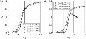
Figure 11. Cross-stream profiles of the scalar correlation coefficient. The downstream locations are given in the legend.
The cross-stream profiles of the correlation coefficient are shown in figure 11. The correlation coefficient generally has values close to negative one close to the centreline, increasing toward unity far away from the centreline. The differences between cases I and II and between cases III and IV are small. As discussed in § 3.3, there are significant differences between the JPDFs and conditional diffusion for the cases I (III) and II (IV), again an indication of the limitations of the correlation coefficient in representing the state of mixing. Comparisons between cases I and III and between cases II and IV show that the evolution of the correlation coefficient is slower for the larger annulus than for the smaller annulus. Note that the decrease for
 $r/d>0.8$
at
$r/d>0.8$
at
 $x/d=3.29$
for the larger annulus cases is because near the jet exit the scalar variances and covariance are very small toward the edge of the jet; therefore the results are affected by the residual noise after the noise correction.
$x/d=3.29$
for the larger annulus cases is because near the jet exit the scalar variances and covariance are very small toward the edge of the jet; therefore the results are affected by the residual noise after the noise correction.

Figure 12. Cross-stream profiles of the segregation parameter. The downstream locations are given in the legend.
The cross-stream profiles of the segregation parameter are shown in figure 12. For all the cases, the segregation parameter is negative close to the centreline because
 $\unicode[STIX]{x1D719}_{1}$
and
$\unicode[STIX]{x1D719}_{1}$
and
 $\unicode[STIX]{x1D719}_{2}$
are negatively correlated. (It is zero on the centreline very close to the jet exit. See Cai et al.
Reference Cai, Dinger, Li, Carter, Ryan and Tong2011.) The
$\unicode[STIX]{x1D719}_{2}$
are negatively correlated. (It is zero on the centreline very close to the jet exit. See Cai et al.
Reference Cai, Dinger, Li, Carter, Ryan and Tong2011.) The
 $\unicode[STIX]{x1D6FC}$
values are generally larger for case I than case II when
$\unicode[STIX]{x1D6FC}$
values are generally larger for case I than case II when
 $r/d>0.8$
, probably because the mixing between
$r/d>0.8$
, probably because the mixing between
 $\unicode[STIX]{x1D719}_{1}$
and
$\unicode[STIX]{x1D719}_{1}$
and
 $\unicode[STIX]{x1D719}_{2}$
is slower for case I. For the larger annulus, the profiles generally have off-centreline minima. The difference between case III and case IV are small. Comparisons between cases I and III and between cases II and IV show that
$\unicode[STIX]{x1D719}_{2}$
is slower for case I. For the larger annulus, the profiles generally have off-centreline minima. The difference between case III and case IV are small. Comparisons between cases I and III and between cases II and IV show that
 $\unicode[STIX]{x1D6FC}$
increases faster for the smaller annulus. Similar to
$\unicode[STIX]{x1D6FC}$
increases faster for the smaller annulus. Similar to
 $\unicode[STIX]{x1D70C}$
,
$\unicode[STIX]{x1D70C}$
,
 $\unicode[STIX]{x1D6FC}$
decreases for
$\unicode[STIX]{x1D6FC}$
decreases for
 $r/d>0.8$
at
$r/d>0.8$
at
 $x/d=3.29$
, because of the residual noise as well as the very small value of
$x/d=3.29$
, because of the residual noise as well as the very small value of
 $\langle \unicode[STIX]{x1D719}_{1}\rangle$
there.
$\langle \unicode[STIX]{x1D719}_{1}\rangle$
there.

Figure 13. Cross-stream profiles of the mean scalar dissipation rates and the mean cross-dissipation rate.
The cross-stream profiles of the mean scalar dissipation rates and mean cross-dissipation rate are shown in figure 13. The peak value of
 $\unicode[STIX]{x1D719}_{1}$
mean dissipation rate,
$\unicode[STIX]{x1D719}_{1}$
mean dissipation rate,
 $\langle \unicode[STIX]{x1D712}_{1}\rangle$
, is larger for case I (III) than case II (IV), because of the larger production rate of
$\langle \unicode[STIX]{x1D712}_{1}\rangle$
, is larger for case I (III) than case II (IV), because of the larger production rate of
 $\unicode[STIX]{x1D70E}_{1}^{2}$
due to the larger
$\unicode[STIX]{x1D70E}_{1}^{2}$
due to the larger
 $\langle \unicode[STIX]{x1D719}_{1}\rangle$
gradient. It decreases faster downstream for cases II and IV, again indicating the faster progression of mixing. The
$\langle \unicode[STIX]{x1D719}_{1}\rangle$
gradient. It decreases faster downstream for cases II and IV, again indicating the faster progression of mixing. The
 $\unicode[STIX]{x1D719}_{2}$
mean dissipation rate,
$\unicode[STIX]{x1D719}_{2}$
mean dissipation rate,
 $\langle \unicode[STIX]{x1D712}_{2}\rangle$
, values are also larger for case I (III) than case II (IV) at all radial locations, again consistent with the larger production rate of
$\langle \unicode[STIX]{x1D712}_{2}\rangle$
, values are also larger for case I (III) than case II (IV) at all radial locations, again consistent with the larger production rate of
 $\unicode[STIX]{x1D70E}_{2}^{2}$
for case I. It is interesting that the mean shear between the
$\unicode[STIX]{x1D70E}_{2}^{2}$
for case I. It is interesting that the mean shear between the
 $\unicode[STIX]{x1D719}_{1}$
–
$\unicode[STIX]{x1D719}_{1}$
–
 $\unicode[STIX]{x1D719}_{2}$
streams for case II does not result in higher
$\unicode[STIX]{x1D719}_{2}$
streams for case II does not result in higher
 $\langle \unicode[STIX]{x1D712}_{1}\rangle$
and
$\langle \unicode[STIX]{x1D712}_{1}\rangle$
and
 $\langle \unicode[STIX]{x1D712}_{2}\rangle$
(left peak) values. The peak value (maximum magnitude) of the mean cross-dissipation rate between
$\langle \unicode[STIX]{x1D712}_{2}\rangle$
(left peak) values. The peak value (maximum magnitude) of the mean cross-dissipation rate between
 $\unicode[STIX]{x1D719}_{1}$
and
$\unicode[STIX]{x1D719}_{1}$
and
 $\unicode[STIX]{x1D719}_{2}$
,
$\unicode[STIX]{x1D719}_{2}$
,
 $\langle \unicode[STIX]{x1D712}_{12}\rangle$
, for case I (III) is also larger than case II (IV), which is a result of larger mean gradients for both
$\langle \unicode[STIX]{x1D712}_{12}\rangle$
, for case I (III) is also larger than case II (IV), which is a result of larger mean gradients for both
 $\unicode[STIX]{x1D719}_{1}$
and
$\unicode[STIX]{x1D719}_{1}$
and
 $\unicode[STIX]{x1D719}_{2}$
.
$\unicode[STIX]{x1D719}_{2}$
.
The peak values of
 $\langle \unicode[STIX]{x1D712}_{1}\rangle$
are slightly larger for the smaller annulus than for the larger annulus at
$\langle \unicode[STIX]{x1D712}_{1}\rangle$
are slightly larger for the smaller annulus than for the larger annulus at
 $x/d=3.29$
. However, they are smaller at
$x/d=3.29$
. However, they are smaller at
 $x/d=6.99$
. The peak values of
$x/d=6.99$
. The peak values of
 $\langle \unicode[STIX]{x1D712}_{2}\rangle$
and
$\langle \unicode[STIX]{x1D712}_{2}\rangle$
and
 $\langle \unicode[STIX]{x1D712}_{12}\rangle$
are generally much smaller for the smaller annulus and the peak values decay faster downstream for the smaller annulus. Moving downstream the peak locations generally also shift (both inward and outward) faster for the smaller annulus, also suggesting faster progression of mixing for the smaller annulus.
$\langle \unicode[STIX]{x1D712}_{12}\rangle$
are generally much smaller for the smaller annulus and the peak values decay faster downstream for the smaller annulus. Moving downstream the peak locations generally also shift (both inward and outward) faster for the smaller annulus, also suggesting faster progression of mixing for the smaller annulus.

Figure 14. Cross-stream profiles of the scalar dissipation time scales.
The scalar dissipation time scale profiles are shown in figure 14. The time scale of
 $\unicode[STIX]{x1D719}_{1}$
,
$\unicode[STIX]{x1D719}_{1}$
,
 $\langle \unicode[STIX]{x1D719}_{1}^{\prime 2}\rangle /\langle \unicode[STIX]{x1D712}_{1}\rangle$
, is generally larger than the time scale of
$\langle \unicode[STIX]{x1D719}_{1}^{\prime 2}\rangle /\langle \unicode[STIX]{x1D712}_{1}\rangle$
, is generally larger than the time scale of
 $\unicode[STIX]{x1D719}_{2}$
,
$\unicode[STIX]{x1D719}_{2}$
,
 $\langle \unicode[STIX]{x1D719}_{2}^{\prime 2}\rangle /\langle \unicode[STIX]{x1D712}_{2}\rangle$
, for all cases. The scalar time scale generally increases with the downstream distance as the jet width grows. The cross-stream variations of the time scales are generally small, similar to two scalar mixing in turbulent jets (Panchapakesan & Lumley Reference Panchapakesan and Lumley1993), except at locations far away from the centreline (
$\langle \unicode[STIX]{x1D719}_{2}^{\prime 2}\rangle /\langle \unicode[STIX]{x1D712}_{2}\rangle$
, for all cases. The scalar time scale generally increases with the downstream distance as the jet width grows. The cross-stream variations of the time scales are generally small, similar to two scalar mixing in turbulent jets (Panchapakesan & Lumley Reference Panchapakesan and Lumley1993), except at locations far away from the centreline (
 $r/d>0.8$
) where the scalar mean dissipation rates are small (less than 10 % of the peak value) and are susceptible to measurement uncertainties. The time scale profiles for cases I(III) and II(IV) do not show significant differences. Comparisons between cases I(II) and III(IV) also do not show significant differences.
$r/d>0.8$
) where the scalar mean dissipation rates are small (less than 10 % of the peak value) and are susceptible to measurement uncertainties. The time scale profiles for cases I(III) and II(IV) do not show significant differences. Comparisons between cases I(II) and III(IV) also do not show significant differences.

Figure 15. Cross-stream evolution of the scalar JPDF at
 $x/d=3.29$
for the smaller annulus. Case I: (a,c,e), case II: (b,d,f). The radial location is given in the top of each figure.
$x/d=3.29$
for the smaller annulus. Case I: (a,c,e), case II: (b,d,f). The radial location is given in the top of each figure.
3.3 Cross-stream JPDF, conditional diffusion, and conditional dissipation
The JPDF for
 $x/d=3.29$
at three radial locations for the smaller annulus are shown in figure 15. As shown in Cai et al. (Reference Cai, Dinger, Li, Carter, Ryan and Tong2011), on the centreline the mixture is essentially pure
$x/d=3.29$
at three radial locations for the smaller annulus are shown in figure 15. As shown in Cai et al. (Reference Cai, Dinger, Li, Carter, Ryan and Tong2011), on the centreline the mixture is essentially pure
 $\unicode[STIX]{x1D719}_{1}$
. Moving away from the centreline, the JPDF extends toward
$\unicode[STIX]{x1D719}_{1}$
. Moving away from the centreline, the JPDF extends toward
 $(0,1)$
along the
$(0,1)$
along the
 $\unicode[STIX]{x1D719}_{1}$
–
$\unicode[STIX]{x1D719}_{1}$
–
 $\unicode[STIX]{x1D719}_{2}$
mixing line and then begins to bend toward
$\unicode[STIX]{x1D719}_{2}$
mixing line and then begins to bend toward
 $(0,0)$
. At
$(0,0)$
. At
 $r/d=0.372$
, the JPDF occupies a larger area in the scalar space for case I than for case II, a result of the stronger large-scale transport (flapping) for case I.
$r/d=0.372$
, the JPDF occupies a larger area in the scalar space for case I than for case II, a result of the stronger large-scale transport (flapping) for case I.
Near the peak location of
 $\unicode[STIX]{x1D70E}_{1}$
profile (e.g.
$\unicode[STIX]{x1D70E}_{1}$
profile (e.g.
 $r/d=0.521$
), the JPDF is bimodal for case I with peaks at (0.4, 0.5) and (0.10, 0.50), representing the
$r/d=0.521$
), the JPDF is bimodal for case I with peaks at (0.4, 0.5) and (0.10, 0.50), representing the
 $\unicode[STIX]{x1D719}_{1}$
–
$\unicode[STIX]{x1D719}_{1}$
–
 $\unicode[STIX]{x1D719}_{2}$
and
$\unicode[STIX]{x1D719}_{2}$
and
 $\unicode[STIX]{x1D719}_{2}$
–
$\unicode[STIX]{x1D719}_{2}$
–
 $\unicode[STIX]{x1D719}_{3}$
mixtures coming from the two mixing layers. The strong transport also results in larger fluctuations in the
$\unicode[STIX]{x1D719}_{3}$
mixtures coming from the two mixing layers. The strong transport also results in larger fluctuations in the
 $\unicode[STIX]{x1D719}_{2}$
–
$\unicode[STIX]{x1D719}_{2}$
–
 $\unicode[STIX]{x1D719}_{3}$
mixture. There is little mixing between
$\unicode[STIX]{x1D719}_{3}$
mixture. There is little mixing between
 $\unicode[STIX]{x1D719}_{1}$
and
$\unicode[STIX]{x1D719}_{1}$
and
 $\unicode[STIX]{x1D719}_{3}$
, however. The bimodal JPDF is again a result of the transport of the two mixtures by the large-scale velocity fluctuations (flapping) generated by the single but stronger shear layer, and the relatively poor small-scale mixing due to the lack of a shear layer between the
$\unicode[STIX]{x1D719}_{3}$
, however. The bimodal JPDF is again a result of the transport of the two mixtures by the large-scale velocity fluctuations (flapping) generated by the single but stronger shear layer, and the relatively poor small-scale mixing due to the lack of a shear layer between the
 $\unicode[STIX]{x1D719}_{1}$
and
$\unicode[STIX]{x1D719}_{1}$
and
 $\unicode[STIX]{x1D719}_{2}$
streams. By contrast, the JPDF for case II is unimodal at all radial locations, due to the weaker transport and better small-scale mixing caused by the presence of the shear layer between the
$\unicode[STIX]{x1D719}_{2}$
streams. By contrast, the JPDF for case II is unimodal at all radial locations, due to the weaker transport and better small-scale mixing caused by the presence of the shear layer between the
 $\unicode[STIX]{x1D719}_{1}$
and
$\unicode[STIX]{x1D719}_{1}$
and
 $\unicode[STIX]{x1D719}_{2}$
streams. At
$\unicode[STIX]{x1D719}_{2}$
streams. At
 $r/d=0.703$
, the JPDF for both cases is unimodal and the peak of the JPDF moves close to (0, 0). However, the JPDF peaks at larger
$r/d=0.703$
, the JPDF for both cases is unimodal and the peak of the JPDF moves close to (0, 0). However, the JPDF peaks at larger
 $\unicode[STIX]{x1D719}_{1}$
values for case II, likely due to the larger advection by the mean flow. Moving further outside, the ridgeline of the JPDF becomes a straight line with a positive slope for both cases.
$\unicode[STIX]{x1D719}_{1}$
values for case II, likely due to the larger advection by the mean flow. Moving further outside, the ridgeline of the JPDF becomes a straight line with a positive slope for both cases.

Figure 16. Cross-stream evolution of the scalar conditional diffusion at
 $x/d=3.29$
for the smaller annulus. Case I: (a,c,e), case II: (b,d,f). The contour magnitudes of the diffusion are the Euclidean norm of the diffusion velocity vector. The mean scalars (
$x/d=3.29$
for the smaller annulus. Case I: (a,c,e), case II: (b,d,f). The contour magnitudes of the diffusion are the Euclidean norm of the diffusion velocity vector. The mean scalars (
 $\langle \unicode[STIX]{x1D719}_{1}\rangle ,\langle \unicode[STIX]{x1D719}_{2}\rangle$
) are indicated in each streamline plot by a solid circle.
$\langle \unicode[STIX]{x1D719}_{1}\rangle ,\langle \unicode[STIX]{x1D719}_{2}\rangle$
) are indicated in each streamline plot by a solid circle.
The conditional scalar diffusion,
 $\langle D_{1}\unicode[STIX]{x1D6FB}^{2}\unicode[STIX]{x1D719}_{1}|\unicode[STIX]{x1D719}_{1},\unicode[STIX]{x1D719}_{2}\rangle$
and
$\langle D_{1}\unicode[STIX]{x1D6FB}^{2}\unicode[STIX]{x1D719}_{1}|\unicode[STIX]{x1D719}_{1},\unicode[STIX]{x1D719}_{2}\rangle$
and
 $\langle D_{2}\unicode[STIX]{x1D6FB}^{2}\unicode[STIX]{x1D719}_{2}|\unicode[STIX]{x1D719}_{1},\unicode[STIX]{x1D719}_{2}\rangle$
, for
$\langle D_{2}\unicode[STIX]{x1D6FB}^{2}\unicode[STIX]{x1D719}_{2}|\unicode[STIX]{x1D719}_{1},\unicode[STIX]{x1D719}_{2}\rangle$
, for
 $x/d=3.29$
at three radial locations for the smaller annulus is shown in figure 16. Since these diffusion terms transport the JPDF in the
$x/d=3.29$
at three radial locations for the smaller annulus is shown in figure 16. Since these diffusion terms transport the JPDF in the
 $\unicode[STIX]{x1D719}_{1}$
–
$\unicode[STIX]{x1D719}_{1}$
–
 $\unicode[STIX]{x1D719}_{2}$
scalar space and are two components of a diffusion velocity, we use diffusion streamlines to represent them. We use the mean dissipation rate and r.m.s. fluctuations of
$\unicode[STIX]{x1D719}_{2}$
scalar space and are two components of a diffusion velocity, we use diffusion streamlines to represent them. We use the mean dissipation rate and r.m.s. fluctuations of
 $\unicode[STIX]{x1D719}_{1}$
to non-dimensionalize the magnitude of the diffusion velocity. The mean composition, (
$\unicode[STIX]{x1D719}_{1}$
to non-dimensionalize the magnitude of the diffusion velocity. The mean composition, (
 $\langle \unicode[STIX]{x1D719}_{1}\rangle$
,
$\langle \unicode[STIX]{x1D719}_{1}\rangle$
,
 $\langle \unicode[STIX]{x1D719}_{2}\rangle$
), is represented by a solid circle in the diffusion streamline plot. Close to the centreline (not shown), the diffusion streamlines generally converge towards the
$\langle \unicode[STIX]{x1D719}_{2}\rangle$
), is represented by a solid circle in the diffusion streamline plot. Close to the centreline (not shown), the diffusion streamlines generally converge towards the
 $\unicode[STIX]{x1D719}_{1}$
–
$\unicode[STIX]{x1D719}_{1}$
–
 $\unicode[STIX]{x1D719}_{2}$
mixing line because the conditional diffusion is small and the measurement is dominated by the measurement uncertainties. Moving away from the centreline, a manifold, towards which the diffusion streamlines first converge to, begins to emerge first for case I and then for case II.
$\unicode[STIX]{x1D719}_{2}$
mixing line because the conditional diffusion is small and the measurement is dominated by the measurement uncertainties. Moving away from the centreline, a manifold, towards which the diffusion streamlines first converge to, begins to emerge first for case I and then for case II.
At
 $r/d=0.521$
, there are well defined and convex-shaped diffusion manifolds for both cases, which are close to the ridgelines of the JPDFs. The curvature of the manifold is much larger for case I than case II, again indicating a lesser degree of mixing for case I, because mixing will eventually lead to a straight JPDF ridgeline (well correlated
$r/d=0.521$
, there are well defined and convex-shaped diffusion manifolds for both cases, which are close to the ridgelines of the JPDFs. The curvature of the manifold is much larger for case I than case II, again indicating a lesser degree of mixing for case I, because mixing will eventually lead to a straight JPDF ridgeline (well correlated
 $\unicode[STIX]{x1D719}_{1}$
and
$\unicode[STIX]{x1D719}_{1}$
and
 $\unicode[STIX]{x1D719}_{2}$
) and a straight mixing line. The JPDF appears to be more symmetric with respect to the manifold in the
$\unicode[STIX]{x1D719}_{2}$
) and a straight mixing line. The JPDF appears to be more symmetric with respect to the manifold in the
 $\unicode[STIX]{x1D719}_{2}$
direction for case II, while it extends further in the direction of lower
$\unicode[STIX]{x1D719}_{2}$
direction for case II, while it extends further in the direction of lower
 $\unicode[STIX]{x1D719}_{2}$
values for case I, i.e. the fluctuations of
$\unicode[STIX]{x1D719}_{2}$
values for case I, i.e. the fluctuations of
 $\unicode[STIX]{x1D719}_{2}$
conditional on
$\unicode[STIX]{x1D719}_{2}$
conditional on
 $\unicode[STIX]{x1D719}_{1}$
is skewed toward small
$\unicode[STIX]{x1D719}_{1}$
is skewed toward small
 $\unicode[STIX]{x1D719}_{2}$
values. This may be due to the uneven mixing on the two sides of the annular stream for case I, with large mean shear on one side of the
$\unicode[STIX]{x1D719}_{2}$
values. This may be due to the uneven mixing on the two sides of the annular stream for case I, with large mean shear on one side of the
 $\unicode[STIX]{x1D719}_{2}$
stream, bringing in the co-flow air and generating large negative
$\unicode[STIX]{x1D719}_{2}$
stream, bringing in the co-flow air and generating large negative
 $\unicode[STIX]{x1D719}_{2}$
fluctuations. Since there is mean shear on both sides of the
$\unicode[STIX]{x1D719}_{2}$
fluctuations. Since there is mean shear on both sides of the
 $\unicode[STIX]{x1D719}_{2}$
stream for case II, the fluctuations of
$\unicode[STIX]{x1D719}_{2}$
stream for case II, the fluctuations of
 $\unicode[STIX]{x1D719}_{2}$
are more symmetric with respect to the manifold. The solid circle (mean scalar values) is well below the manifold for case I while it is closer to the manifold for case II, consistent with faster mixing for case II. Thus mixing does not transport the scalars toward their mean values. The manifold is actually close to the conditional mean,
$\unicode[STIX]{x1D719}_{2}$
are more symmetric with respect to the manifold. The solid circle (mean scalar values) is well below the manifold for case I while it is closer to the manifold for case II, consistent with faster mixing for case II. Thus mixing does not transport the scalars toward their mean values. The manifold is actually close to the conditional mean,
 $\langle \unicode[STIX]{x1D719}_{2}|\unicode[STIX]{x1D719}_{1}\rangle$
, and its separation from the mean scalars is an important consequence of the three-scalar flow configuration. They become closer as the mixing process progresses. At
$\langle \unicode[STIX]{x1D719}_{2}|\unicode[STIX]{x1D719}_{1}\rangle$
, and its separation from the mean scalars is an important consequence of the three-scalar flow configuration. They become closer as the mixing process progresses. At
 $r/d=0.703$
, the diffusion streamline patterns are the opposite of those close the centreline.
$r/d=0.703$
, the diffusion streamline patterns are the opposite of those close the centreline.

Figure 17. Conditional dissipation rate and conditional cross-dissipation rate at
 $x/d=3.29$
and
$x/d=3.29$
and
 $r/d=0.521$
for the smaller annulus. Case I: (a,c,e), case II: (b,d,f). (a,b), (c,d), (e,f) are for
$r/d=0.521$
for the smaller annulus. Case I: (a,c,e), case II: (b,d,f). (a,b), (c,d), (e,f) are for
 $\langle \unicode[STIX]{x1D712}_{1}|\unicode[STIX]{x1D719}_{1},\unicode[STIX]{x1D719}_{2}\rangle$
,
$\langle \unicode[STIX]{x1D712}_{1}|\unicode[STIX]{x1D719}_{1},\unicode[STIX]{x1D719}_{2}\rangle$
,
 $\langle \unicode[STIX]{x1D712}_{2}|\unicode[STIX]{x1D719}_{1},\unicode[STIX]{x1D719}_{2}\rangle$
and
$\langle \unicode[STIX]{x1D712}_{2}|\unicode[STIX]{x1D719}_{1},\unicode[STIX]{x1D719}_{2}\rangle$
and
 $\langle \unicode[STIX]{x1D712}_{12}|\unicode[STIX]{x1D719}_{1},\unicode[STIX]{x1D719}_{2}\rangle$
, respectively.
$\langle \unicode[STIX]{x1D712}_{12}|\unicode[STIX]{x1D719}_{1},\unicode[STIX]{x1D719}_{2}\rangle$
, respectively.
The conditional dissipation rates of
 $\unicode[STIX]{x1D719}_{1}$
and
$\unicode[STIX]{x1D719}_{1}$
and
 $\unicode[STIX]{x1D719}_{2}$
,
$\unicode[STIX]{x1D719}_{2}$
,
 $\langle \unicode[STIX]{x1D712}_{1}|\unicode[STIX]{x1D719}_{1},\unicode[STIX]{x1D719}_{2}\rangle$
and
$\langle \unicode[STIX]{x1D712}_{1}|\unicode[STIX]{x1D719}_{1},\unicode[STIX]{x1D719}_{2}\rangle$
and
 $\langle \unicode[STIX]{x1D712}_{2}|\unicode[STIX]{x1D719}_{1},\unicode[STIX]{x1D719}_{2}\rangle$
, and the conditional cross-dissipation rate,
$\langle \unicode[STIX]{x1D712}_{2}|\unicode[STIX]{x1D719}_{1},\unicode[STIX]{x1D719}_{2}\rangle$
, and the conditional cross-dissipation rate,
 $\langle \unicode[STIX]{x1D712}_{12}|\unicode[STIX]{x1D719}_{1},\unicode[STIX]{x1D719}_{2}\rangle$
, are non-dimensionalized by the maximum mean dissipation rate of
$\langle \unicode[STIX]{x1D712}_{12}|\unicode[STIX]{x1D719}_{1},\unicode[STIX]{x1D719}_{2}\rangle$
, are non-dimensionalized by the maximum mean dissipation rate of
 $\unicode[STIX]{x1D719}_{1}$
at the same
$\unicode[STIX]{x1D719}_{1}$
at the same
 $x/d$
location. For the smaller annulus at
$x/d$
location. For the smaller annulus at
 $x/d=3.29$
, the general forms of the dissipation rates are similar to those shown in Cai et al. (Reference Cai, Dinger, Li, Carter, Ryan and Tong2011). Figure 17 shows the rates at
$x/d=3.29$
, the general forms of the dissipation rates are similar to those shown in Cai et al. (Reference Cai, Dinger, Li, Carter, Ryan and Tong2011). Figure 17 shows the rates at
 $r/d=0.521$
. Here
$r/d=0.521$
. Here
 $\langle \unicode[STIX]{x1D712}_{1}|\unicode[STIX]{x1D719}_{1},\unicode[STIX]{x1D719}_{2}\rangle$
has a single peak (near (0.44, 0.3)) with values comparable for both cases. There are two peaks for
$\langle \unicode[STIX]{x1D712}_{1}|\unicode[STIX]{x1D719}_{1},\unicode[STIX]{x1D719}_{2}\rangle$
has a single peak (near (0.44, 0.3)) with values comparable for both cases. There are two peaks for
 $\langle \unicode[STIX]{x1D712}_{2}|\unicode[STIX]{x1D719}_{1},\unicode[STIX]{x1D719}_{2}\rangle$
. The right peak is close to the peak location of
$\langle \unicode[STIX]{x1D712}_{2}|\unicode[STIX]{x1D719}_{1},\unicode[STIX]{x1D719}_{2}\rangle$
. The right peak is close to the peak location of
 $\langle \unicode[STIX]{x1D712}_{1}|\unicode[STIX]{x1D719}_{1},\unicode[STIX]{x1D719}_{2}\rangle$
, because it also results from the mixing between
$\langle \unicode[STIX]{x1D712}_{1}|\unicode[STIX]{x1D719}_{1},\unicode[STIX]{x1D719}_{2}\rangle$
, because it also results from the mixing between
 $\unicode[STIX]{x1D719}_{1}$
and
$\unicode[STIX]{x1D719}_{1}$
and
 $\unicode[STIX]{x1D719}_{2}$
–
$\unicode[STIX]{x1D719}_{2}$
–
 $\unicode[STIX]{x1D719}_{3}$
mixture. As a result,
$\unicode[STIX]{x1D719}_{3}$
mixture. As a result,
 $\langle \unicode[STIX]{x1D712}_{12}|\unicode[STIX]{x1D719}_{1},\unicode[STIX]{x1D719}_{2}\rangle$
has a negative peak there. Near the left end of the JPDF
$\langle \unicode[STIX]{x1D712}_{12}|\unicode[STIX]{x1D719}_{1},\unicode[STIX]{x1D719}_{2}\rangle$
has a negative peak there. Near the left end of the JPDF
 $\langle \unicode[STIX]{x1D712}_{2}|\unicode[STIX]{x1D719}_{1},\unicode[STIX]{x1D719}_{2}\rangle$
is also comparable for both cases, in spite of the larger
$\langle \unicode[STIX]{x1D712}_{2}|\unicode[STIX]{x1D719}_{1},\unicode[STIX]{x1D719}_{2}\rangle$
is also comparable for both cases, in spite of the larger
 $\unicode[STIX]{x1D719}_{2}$
fluctuations. The conditional dissipation rates for the mixture fraction and temperature in a non-premixed (or partially premixed) flame also have a single peak and two peaks respectively (Cai et al.
Reference Cai, Wang, Tong, Barlow and Karpetis2009), due to the similarity between the scalar configurations for the coaxial jets and non-premixed reactive flows. Despite of the stronger transport of the JPDF creating large (conditional) fluctuations, the conditional dissipation rates have comparable magnitudes for the two cases; therefore, mixing for case I does not keep pace with production, delaying the evolution of the JPDF.
$\unicode[STIX]{x1D719}_{2}$
fluctuations. The conditional dissipation rates for the mixture fraction and temperature in a non-premixed (or partially premixed) flame also have a single peak and two peaks respectively (Cai et al.
Reference Cai, Wang, Tong, Barlow and Karpetis2009), due to the similarity between the scalar configurations for the coaxial jets and non-premixed reactive flows. Despite of the stronger transport of the JPDF creating large (conditional) fluctuations, the conditional dissipation rates have comparable magnitudes for the two cases; therefore, mixing for case I does not keep pace with production, delaying the evolution of the JPDF.

Figure 18. Conditions same as figure 15 but at
 $x/d=6.99$
.
$x/d=6.99$
.
Moving downstream to
 $x/d=6.99$
, the JPDF has already bent down toward
$x/d=6.99$
, the JPDF has already bent down toward
 $(0,0)$
on the centreline for both cases (figure 7) with case II bending further. The JPDF is again bimodal near the peak location of
$(0,0)$
on the centreline for both cases (figure 7) with case II bending further. The JPDF is again bimodal near the peak location of
 $\unicode[STIX]{x1D70E}_{1}$
profile (e.g.
$\unicode[STIX]{x1D70E}_{1}$
profile (e.g.
 $r/d=0.376$
) for case I (figure 18). However, the curvature of the ridgeline of the JPDF is smaller than at the upstream location (
$r/d=0.376$
) for case I (figure 18). However, the curvature of the ridgeline of the JPDF is smaller than at the upstream location (
 $x/d=3.29$
and
$x/d=3.29$
and
 $r/d=0.521$
), due to the progression of the mixing process. The JPDF is again unimodal for case II at all radial locations. At
$r/d=0.521$
), due to the progression of the mixing process. The JPDF is again unimodal for case II at all radial locations. At
 $r/d=0.538$
, the forms of the JPDF for the two cases are quite different, with case II having smaller
$r/d=0.538$
, the forms of the JPDF for the two cases are quite different, with case II having smaller
 $\unicode[STIX]{x1D719}_{2}$
fluctuations, due to better small-scale mixing resulting from the two shear layers. Further away from the centreline the ridgeline of the JPDF becomes a straight line.
$\unicode[STIX]{x1D719}_{2}$
fluctuations, due to better small-scale mixing resulting from the two shear layers. Further away from the centreline the ridgeline of the JPDF becomes a straight line.

Figure 19. Conditions same as figure 16 but at
 $x/d=6.99$
.
$x/d=6.99$
.
The conditional diffusion streamlines at
 $x/d=6.99$
(figure 19) have general patterns similar to those at
$x/d=6.99$
(figure 19) have general patterns similar to those at
 $x/d=3.29$
. The manifold is already well defined even on the centreline. For both cases I and II, the curvature of the manifold is smaller at
$x/d=3.29$
. The manifold is already well defined even on the centreline. For both cases I and II, the curvature of the manifold is smaller at
 $x/d=6.99$
than at
$x/d=6.99$
than at
 $x/d=3.29$
and the mean composition (the solid circle) is closer to the manifold. The curvature of the manifold is larger for case I than case II, again indicating a lesser degree of mixing for case I. The JPDF is somewhat skewed toward smaller
$x/d=3.29$
and the mean composition (the solid circle) is closer to the manifold. The curvature of the manifold is larger for case I than case II, again indicating a lesser degree of mixing for case I. The JPDF is somewhat skewed toward smaller
 $\unicode[STIX]{x1D719}_{2}$
values for case I, while it is quite symmetric with respect to the manifold for case II.
$\unicode[STIX]{x1D719}_{2}$
values for case I, while it is quite symmetric with respect to the manifold for case II.

Figure 20. Cross-stream evolution of the scalar JPDF at
 $x/d=3.29$
for the larger annulus. Case III: (a,c), case IV: (b,d).
$x/d=3.29$
for the larger annulus. Case III: (a,c), case IV: (b,d).
The JPDF at
 $x/d=3.29$
for the larger annulus (cases III and IV) are shown in figure 20. On the centreline, the mixture is again essentially pure
$x/d=3.29$
for the larger annulus (cases III and IV) are shown in figure 20. On the centreline, the mixture is again essentially pure
 $\unicode[STIX]{x1D719}_{1}$
. Near the centreline, the JPDF has a long tail toward
$\unicode[STIX]{x1D719}_{1}$
. Near the centreline, the JPDF has a long tail toward
 $(0,1)$
while the peak is still close to
$(0,1)$
while the peak is still close to
 $(1,0)$
for both cases. At
$(1,0)$
for both cases. At
 $r/d=0.448$
, the ridgeline of the JPDF connects
$r/d=0.448$
, the ridgeline of the JPDF connects
 $(0,1)$
and
$(0,1)$
and
 $(1,0)$
, a result of the turbulent transport (flapping of the
$(1,0)$
, a result of the turbulent transport (flapping of the
 $\unicode[STIX]{x1D719}_{1}$
–
$\unicode[STIX]{x1D719}_{1}$
–
 $\unicode[STIX]{x1D719}_{2}$
mixing layer). At
$\unicode[STIX]{x1D719}_{2}$
mixing layer). At
 $r/d=0.662$
, while its peak is very close to
$r/d=0.662$
, while its peak is very close to
 $(0,1)$
, the JPDF has tails pointing toward both
$(0,1)$
, the JPDF has tails pointing toward both
 $(0,0)$
and
$(0,0)$
and
 $(1,0)$
, indicating that nearly pure
$(1,0)$
, indicating that nearly pure
 $\unicode[STIX]{x1D719}_{2}$
mixture is mixing with
$\unicode[STIX]{x1D719}_{2}$
mixture is mixing with
 $\unicode[STIX]{x1D719}_{1}$
and
$\unicode[STIX]{x1D719}_{1}$
and
 $\unicode[STIX]{x1D719}_{3}$
separately. There is little direct mixing between
$\unicode[STIX]{x1D719}_{3}$
separately. There is little direct mixing between
 $\unicode[STIX]{x1D719}_{1}$
and
$\unicode[STIX]{x1D719}_{1}$
and
 $\unicode[STIX]{x1D719}_{3}$
because they are separated by nearly pure
$\unicode[STIX]{x1D719}_{3}$
because they are separated by nearly pure
 $\unicode[STIX]{x1D719}_{2}$
. The lower values of
$\unicode[STIX]{x1D719}_{2}$
. The lower values of
 $\unicode[STIX]{x1D719}_{2}$
for case IV are due to the faster mixing. The ‘corner’ of the JPDF near
$\unicode[STIX]{x1D719}_{2}$
for case IV are due to the faster mixing. The ‘corner’ of the JPDF near
 $(0,1)$
is sharper for case III (IV) than for case I (II). The tail toward
$(0,1)$
is sharper for case III (IV) than for case I (II). The tail toward
 $(0,0)$
becomes longer and the tail toward
$(0,0)$
becomes longer and the tail toward
 $(1,0)$
becomes shorter when moving further away from the centreline (not shown). The peak of JPDF also leaves
$(1,0)$
becomes shorter when moving further away from the centreline (not shown). The peak of JPDF also leaves
 $(0,1)$
and moves toward
$(0,1)$
and moves toward
 $(0,0)$
.
$(0,0)$
.

Figure 21. Scalar conditional diffusion at
 $x/d=3.29$
and
$x/d=3.29$
and
 $r/d=0.662$
for the larger annulus. Case III: (a), case IV: (b).
$r/d=0.662$
for the larger annulus. Case III: (a), case IV: (b).
The conditional diffusion at
 $x/d=3.29$
and
$x/d=3.29$
and
 $r/d=0.662$
for cases III and IV is shown in figure 21. Diffusion streamlines at other radial locations are not shown because they are dominated by measurement uncertainties. At
$r/d=0.662$
for cases III and IV is shown in figure 21. Diffusion streamlines at other radial locations are not shown because they are dominated by measurement uncertainties. At
 $r/d=0.662$
, the diffusion streamlines mostly converge to the
$r/d=0.662$
, the diffusion streamlines mostly converge to the
 $\unicode[STIX]{x1D719}_{1}$
–
$\unicode[STIX]{x1D719}_{1}$
–
 $\unicode[STIX]{x1D719}_{2}$
mixing line directly. There is no sign of a curved manifold. Here the mixing is still largely binary as
$\unicode[STIX]{x1D719}_{2}$
mixing line directly. There is no sign of a curved manifold. Here the mixing is still largely binary as
 $\unicode[STIX]{x1D719}_{1}$
and
$\unicode[STIX]{x1D719}_{1}$
and
 $\unicode[STIX]{x1D719}_{3}$
are still separated by nearly pure
$\unicode[STIX]{x1D719}_{3}$
are still separated by nearly pure
 $\unicode[STIX]{x1D719}_{2}$
without direct mixing between them, while a curved manifold generally is a result of three-scalar mixing.
$\unicode[STIX]{x1D719}_{2}$
without direct mixing between them, while a curved manifold generally is a result of three-scalar mixing.

Figure 22. Cross-stream evolution of the scalar JPDF at
 $x/d=6.99$
for the larger annulus. Case III: (a,c), case IV: (b,d).
$x/d=6.99$
for the larger annulus. Case III: (a,c), case IV: (b,d).
On the centreline at
 $x/d=6.99$
, the ridgelines of the JPDFs are still close to the
$x/d=6.99$
, the ridgelines of the JPDFs are still close to the
 $\unicode[STIX]{x1D719}_{1}$
–
$\unicode[STIX]{x1D719}_{1}$
–
 $\unicode[STIX]{x1D719}_{2}$
mixing line for both cases III and IV (figure 8). At
$\unicode[STIX]{x1D719}_{2}$
mixing line for both cases III and IV (figure 8). At
 $r/d=0.289$
(figure 22), the JPDF begins to bend toward
$r/d=0.289$
(figure 22), the JPDF begins to bend toward
 $(0,0)$
and extends much further toward
$(0,0)$
and extends much further toward
 $(0,1)$
for case III. Its area is also larger for case III, indicating stronger turbulent transport. Similar to case I, the JPDF for case III is also bimodal near the peak location of
$(0,1)$
for case III. Its area is also larger for case III, indicating stronger turbulent transport. Similar to case I, the JPDF for case III is also bimodal near the peak location of
 $\unicode[STIX]{x1D70E}_{1}$
profile (e.g.
$\unicode[STIX]{x1D70E}_{1}$
profile (e.g.
 $r/d=0.496$
). However, unlike at
$r/d=0.496$
). However, unlike at
 $x/d=3.29$
the peak of JPDF does not reach
$x/d=3.29$
the peak of JPDF does not reach
 $(0,1)$
, a result of the progression of the mixing process. The JPDF is unimodal for case IV at all radial locations. At
$(0,1)$
, a result of the progression of the mixing process. The JPDF is unimodal for case IV at all radial locations. At
 $r/d=0.744$
(not shown), the right peak has disappeared for case III. Moving further outside the general trends of the evolution of the JPDF are similar to those of the smaller annulus cases.
$r/d=0.744$
(not shown), the right peak has disappeared for case III. Moving further outside the general trends of the evolution of the JPDF are similar to those of the smaller annulus cases.

Figure 23. Cross-stream scalar conditional diffusion at
 $x/d=6.99$
and
$x/d=6.99$
and
 $r/d=0.496$
for the larger annulus. Case III: (a), case IV: (b).
$r/d=0.496$
for the larger annulus. Case III: (a), case IV: (b).
The patterns of conditional diffusion streamlines at
 $x/d=6.99$
for the larger annulus (figure 23) are generally similar to those of the smaller annulus cases at
$x/d=6.99$
for the larger annulus (figure 23) are generally similar to those of the smaller annulus cases at
 $x/d=3.29$
. The manifold begins to emerge at
$x/d=3.29$
. The manifold begins to emerge at
 $r/d=0.289$
(figures not shown) and it is well defined at
$r/d=0.289$
(figures not shown) and it is well defined at
 $r/d=0.496$
(figure 23). The curvature of the manifold is larger for case III than case IV. The mean composition is further away from the manifold for case III. The curvature of the manifold for case III at
$r/d=0.496$
(figure 23). The curvature of the manifold is larger for case III than case IV. The mean composition is further away from the manifold for case III. The curvature of the manifold for case III at
 $x/d=6.99$
appears to be larger than for case I at
$x/d=6.99$
appears to be larger than for case I at
 $x/d=3.29$
, consistent with the sharper ‘corner’ of the JPDF. The general trends of the conditional dissipation rates and conditional cross-dissipation rate (figures not shown) for the larger annulus at
$x/d=3.29$
, consistent with the sharper ‘corner’ of the JPDF. The general trends of the conditional dissipation rates and conditional cross-dissipation rate (figures not shown) for the larger annulus at
 $x/d=6.99$
are also similar to those of the smaller annulus.
$x/d=6.99$
are also similar to those of the smaller annulus.
4 Discussion and conclusions
In the present study, we investigated the effects of the velocity ratio (mean shear) and the length scale ratio on three-scalar mixing in turbulent coaxial jets. The velocity ratio alters the relative mean shear rates in the mixing layers between the centre jet and the annular flow and between the annular flow and the co-flow, modifying the scalar fields and the JPDF through mean-flow advection, turbulent transport and small-scale mixing. The length scale ratio determines the degree of separation between the centre jet and the co-flow. The mixing process in this flow better approximates that in turbulent non-premixed reactive flows than those in previous studies. Therefore, the results in the present study advance the understanding of turbulent mixing in reactive flows, and can be used to test mixing models.
For the cases with the higher velocity ratio (cases I and III) the cross-stream mean profiles for
 $\unicode[STIX]{x1D719}_{1}$
are narrower with the centreline values lower (the mean scalar gradient is higher, however), primarily due to the smaller mean-flow advection resulting from the wider mean velocity profile and the slower decay of the centreline velocity. The cross-stream turbulent convection is also larger, further reducing the centreline value. The peak value of
$\unicode[STIX]{x1D719}_{1}$
are narrower with the centreline values lower (the mean scalar gradient is higher, however), primarily due to the smaller mean-flow advection resulting from the wider mean velocity profile and the slower decay of the centreline velocity. The cross-stream turbulent convection is also larger, further reducing the centreline value. The peak value of
 $\langle \unicode[STIX]{x1D719}_{2}\rangle$
, on the other hand, is larger for these higher velocity ratio cases, due to the larger mean advection, although the cross-stream turbulent convection partially counters the mean advection. The r.m.s. scalar fluctuations are larger for both scalars for cases I and III, caused by the larger scalar variance production rates resulting from the larger mean scalar gradients and the higher turbulent fluxes. Thus, shifting the
$\langle \unicode[STIX]{x1D719}_{2}\rangle$
, on the other hand, is larger for these higher velocity ratio cases, due to the larger mean advection, although the cross-stream turbulent convection partially counters the mean advection. The r.m.s. scalar fluctuations are larger for both scalars for cases I and III, caused by the larger scalar variance production rates resulting from the larger mean scalar gradients and the higher turbulent fluxes. Thus, shifting the
 $\unicode[STIX]{x1D719}_{2}$
stream inward relative to the mean shear slows down the overall three-scalar mixing process.
$\unicode[STIX]{x1D719}_{2}$
stream inward relative to the mean shear slows down the overall three-scalar mixing process.
Analyses of the statistics based on the JPDF equation, especially their dependencies on the velocity and length scale ratios, allow us to understand the role played by mean-flow advection, (large-scale) turbulent transport (in physical space), and small-scale mixing (transport in scalar space) in the evolution of the JPDF. The effects of the velocity ratio and length scale ratio on the evolution of the JPDF are a result of their altering the interactions among these contributions.
Detailed analyses show that the peak location of the scalar JPDF (in the scalar space) is generally consistent with the mean scalar values, and therefore is dominated by the mean-flow advection of the JPDF. The larger velocity ratio causes decreased and increased mean-flow advection for
 $\unicode[STIX]{x1D719}_{1}$
and
$\unicode[STIX]{x1D719}_{1}$
and
 $\unicode[STIX]{x1D719}_{2}$
, respectively. It also generates eddies with larger length scales and stronger fluctuations, due to the single but stronger shear layer between
$\unicode[STIX]{x1D719}_{2}$
, respectively. It also generates eddies with larger length scales and stronger fluctuations, due to the single but stronger shear layer between
 $\unicode[STIX]{x1D719}_{2}$
–
$\unicode[STIX]{x1D719}_{2}$
–
 $\unicode[STIX]{x1D719}_{3}$
streams, thereby resulting in stronger large-scale turbulent transport of the JPDF. The conditional dissipation rates, however, are not substantially increased. As a result, the JPDF for these cases is bimodal at some locations, with one peak representing a mixture of
$\unicode[STIX]{x1D719}_{3}$
streams, thereby resulting in stronger large-scale turbulent transport of the JPDF. The conditional dissipation rates, however, are not substantially increased. As a result, the JPDF for these cases is bimodal at some locations, with one peak representing a mixture of
 $\unicode[STIX]{x1D719}_{2}$
and
$\unicode[STIX]{x1D719}_{2}$
and
 $\unicode[STIX]{x1D719}_{3}$
, and the other consisting of mostly
$\unicode[STIX]{x1D719}_{3}$
, and the other consisting of mostly
 $\unicode[STIX]{x1D719}_{1}$
. The bimodal JPDF is due to the poor mixing between
$\unicode[STIX]{x1D719}_{1}$
. The bimodal JPDF is due to the poor mixing between
 $\unicode[STIX]{x1D719}_{1}$
and the
$\unicode[STIX]{x1D719}_{1}$
and the
 $\unicode[STIX]{x1D719}_{2}$
–
$\unicode[STIX]{x1D719}_{2}$
–
 $\unicode[STIX]{x1D719}_{3}$
mixture and the large-scale turbulent transport (flapping). By contrast, the JPDF is always unimodal for the cases with the smaller velocity ratio (II and IV) due to the shear layers on both sides of the
$\unicode[STIX]{x1D719}_{3}$
mixture and the large-scale turbulent transport (flapping). By contrast, the JPDF is always unimodal for the cases with the smaller velocity ratio (II and IV) due to the shear layers on both sides of the
 $\unicode[STIX]{x1D719}_{2}$
stream generating eddies with smaller length scales and weaker fluctuations, thus speeding up the mixing process.
$\unicode[STIX]{x1D719}_{2}$
stream generating eddies with smaller length scales and weaker fluctuations, thus speeding up the mixing process.
Overall, the initial evolution of the scalar fields for the larger velocity ratio is faster due to the stronger transport of the JPDF. However, the shapes of the JPDF indicate that the evolution further downstream is delayed due to the slower small-scale mixing. Furthermore, the larger velocity ratio tends to preserve the initial three-scalar configurations, whereas the smaller velocity ratio results in more effective small-scale mixing, and thus tends to destroy the initial three-scalar configuration. Increasing the length scale ratio delays the progression of the mixing process and makes the effects of the velocity ratio more pronounced.
For all the cases the conditional diffusion streamlines in the scalar space representing the diffusion velocity generally converge quickly to a manifold. The streamline patterns have significant differences for the different velocity ratios. One of the important differences is the curvature of the diffusion manifold. For the cases with the larger velocity ratio (I and III), the curvature is larger with the mean composition farther from of the manifold, further indicating slower progress of the mixing process, since mixing tends to reduce the curvature, and will eventually lead to a straight line manifold with the mean composition on it. The larger annulus width also increases the curvature of the manifold, indicating slower mixing. Another important difference is the location of the manifold in the
 $\unicode[STIX]{x1D719}_{2}$
direction relative to the JPDF. For cases I and III the
$\unicode[STIX]{x1D719}_{2}$
direction relative to the JPDF. For cases I and III the
 $\unicode[STIX]{x1D719}_{2}$
fluctuations are skewed toward smaller values, due to uneven mixing in the two mixing layers. While the existence of the manifold is a result of the configuration of the coaxial jet itself, our analyses show that the different velocity ratios and length scales alter the large-scale turbulent transport and the small-scale mixing, resulting in different curvatures and locations of the manifold.
$\unicode[STIX]{x1D719}_{2}$
fluctuations are skewed toward smaller values, due to uneven mixing in the two mixing layers. While the existence of the manifold is a result of the configuration of the coaxial jet itself, our analyses show that the different velocity ratios and length scales alter the large-scale turbulent transport and the small-scale mixing, resulting in different curvatures and locations of the manifold.
The results in the present study have implications for understanding the mixing process in turbulent reactive flows and mixing models. Varying the velocity ratio alters the location of the peak
 $\langle \unicode[STIX]{x1D719}_{2}\rangle$
value relative to the mean shear, which is analogous to shifting the location of the product, and hence the stoichiometric mixture fraction in a non-premixed reactive flow. Thus, our results suggest that from the three-scalar mixing point of view, increasing the stoichiometric mixture fraction tends to decrease and increase the mean values of the fuel and product, respectively. The bimodal JPDF and the strong peak of
$\langle \unicode[STIX]{x1D719}_{2}\rangle$
value relative to the mean shear, which is analogous to shifting the location of the product, and hence the stoichiometric mixture fraction in a non-premixed reactive flow. Thus, our results suggest that from the three-scalar mixing point of view, increasing the stoichiometric mixture fraction tends to decrease and increase the mean values of the fuel and product, respectively. The bimodal JPDF and the strong peak of
 $\langle \unicode[STIX]{x1D712}_{1}|\unicode[STIX]{x1D719}_{1},\unicode[STIX]{x1D719}_{2}\rangle$
for the cases with the higher velocity ratio indicate that there exists a large jump in the
$\langle \unicode[STIX]{x1D712}_{1}|\unicode[STIX]{x1D719}_{1},\unicode[STIX]{x1D719}_{2}\rangle$
for the cases with the higher velocity ratio indicate that there exists a large jump in the
 $\unicode[STIX]{x1D719}_{1}$
value over a relatively thin layer (ramp-cliff structure) (Tong & Warhaft Reference Tong and Warhaft1995, Tong Reference Tong2001, Wang & Tong Reference Wang and Tong2002, Rajagopalan & Tong Reference Rajagopalan and Tong2003, Wang & Tong Reference Wang and Tong2005). In a turbulent non-premixed flame such a structure tends to result in flamelets (Wang et al.
Reference Wang, Tong, Barlow and Karpetis2007a
, Cai et al.
Reference Cai, Wang, Tong, Barlow and Karpetis2009).
$\unicode[STIX]{x1D719}_{1}$
value over a relatively thin layer (ramp-cliff structure) (Tong & Warhaft Reference Tong and Warhaft1995, Tong Reference Tong2001, Wang & Tong Reference Wang and Tong2002, Rajagopalan & Tong Reference Rajagopalan and Tong2003, Wang & Tong Reference Wang and Tong2005). In a turbulent non-premixed flame such a structure tends to result in flamelets (Wang et al.
Reference Wang, Tong, Barlow and Karpetis2007a
, Cai et al.
Reference Cai, Wang, Tong, Barlow and Karpetis2009).
Varying the length scale ratio alters the relative width of the
 $\unicode[STIX]{x1D719}_{2}$
stream, which from the mixing point of view is analogous to changing the reaction zone width. The results in the present study show that increasing the length scale ratio increases the curvature of the diffusion manifold and makes the ‘corner’ of the JPDF near the peak
$\unicode[STIX]{x1D719}_{2}$
stream, which from the mixing point of view is analogous to changing the reaction zone width. The results in the present study show that increasing the length scale ratio increases the curvature of the diffusion manifold and makes the ‘corner’ of the JPDF near the peak
 $\unicode[STIX]{x1D719}_{2}$
value sharper. When the reaction zone width in a reactive flow is increased (through chemistry), the curvature of the diffusion manifold decreases. The increased length scale slows down the mixing process, which tends to increase the curvature, partially countering the effects of the chemistry.
$\unicode[STIX]{x1D719}_{2}$
value sharper. When the reaction zone width in a reactive flow is increased (through chemistry), the curvature of the diffusion manifold decreases. The increased length scale slows down the mixing process, which tends to increase the curvature, partially countering the effects of the chemistry.
The observed dependence of the mixing process, e.g. the curvature of the diffusion manifold, on the velocity ratio and the annulus width presents a challenging test for mixing models, and provides an important means of evaluating their accuracy. The understanding of the effects of the velocity ratio and length scales can also potentially be used in a design process to achieve a certain desired JPDF shape and other mixing characteristics in turbulent reactive flows by tuning the relative magnitudes of mean-flow advection, turbulent transport and small-scale mixing.
Acknowledgements
The work at Clemson was supported by the National Science Foundation under grant CBET-1333489. We thank Professor S. Pope for valuable discussions.
Appendix. Measurement resolutions of the scalar dissipation rate
To assess the measurement resolution, we used both Rayleigh scattering and LIF to measure
 $\unicode[STIX]{x1D719}_{1}$
by feeding the annular stream with an air flow. While the
$\unicode[STIX]{x1D719}_{1}$
by feeding the annular stream with an air flow. While the
 $\unicode[STIX]{x1D719}_{1}$
mean profiles from the two techniques are essentially the same (figure not shown), the mean scalar dissipation rate, noise corrected using the method of Cai & Tong (Reference Cai and Tong2009), are quite different (figure 24
a). The mean dissipation rate obtained using LIF is lower than using Rayleigh scattering (approximately 40 % at the peak value). Thus the resolutions of the scalar dissipation rate for the two techniques are different. Measurements of the scalar dissipation rate require high spatial resolution. The measurement resolution is affected by several factors including the camera lens resolution, the image pixel size, the finite difference scheme and the laser sheet thickness.
$\unicode[STIX]{x1D719}_{1}$
mean profiles from the two techniques are essentially the same (figure not shown), the mean scalar dissipation rate, noise corrected using the method of Cai & Tong (Reference Cai and Tong2009), are quite different (figure 24
a). The mean dissipation rate obtained using LIF is lower than using Rayleigh scattering (approximately 40 % at the peak value). Thus the resolutions of the scalar dissipation rate for the two techniques are different. Measurements of the scalar dissipation rate require high spatial resolution. The measurement resolution is affected by several factors including the camera lens resolution, the image pixel size, the finite difference scheme and the laser sheet thickness.
The resolution of the camera lens (optical blurring) can be quantified by the line-spread function (LSF) (Wang & Clemens Reference Wang and Clemens2004). We quantified it by translating a razor blade across the imaging plane, using a set-up similar to that in Clemens (Reference Clemens2002). The FWHM of the LSF for the lens arrangement in the present study was approximately
 $38~\unicode[STIX]{x03BC}\text{m}$
. The measurement system resolution is also very sensitive to the camera lens focus, due to the small depth of field resulting from the large magnification ratio and the large aperture (small
$38~\unicode[STIX]{x03BC}\text{m}$
. The measurement system resolution is also very sensitive to the camera lens focus, due to the small depth of field resulting from the large magnification ratio and the large aperture (small
 $f$
-number). We fine tuned the focus by blocking a small part of the laser sheet using a fine metal wire, resulting in a shadow in the acquired images. The fringes resulting from the interference of the light above and below the wire in the neighbourhood of the shadow showed most details when the camera lens was focused.
$f$
-number). We fine tuned the focus by blocking a small part of the laser sheet using a fine metal wire, resulting in a shadow in the acquired images. The fringes resulting from the interference of the light above and below the wire in the neighbourhood of the shadow showed most details when the camera lens was focused.
The camera lens focus is also affected by the wavelength of the light signal. While the wavelength of the Rayleigh scattering signal is the same as the laser light (532 nm), with an extremely small linewidth, the LIF emission from acetone excited at 266 nm is broadband, from 320 nm to 550 nm with the peak at approximately 410 nm (Bryant, Donbar & Driscoll Reference Bryant, Donbar and Driscoll2000). Since the focal length of the camera lens varies with the wavelength, the camera lens is expected to be less well focused for acetone LIF than for Rayleigh scattering. Although we do not have a model to quantify its effects on the resolution of the scalar dissipation, the difference in the quality of the camera lens focus for the two techniques was obvious, with the image of the fringe produced by the fine wire having less details for the 266 nm beam.

Figure 24. Cross-stream profiles of the noise-corrected mean dissipation rate of
 $\unicode[STIX]{x1D719}_{1}$
(a) at
$\unicode[STIX]{x1D719}_{1}$
(a) at
 $x/d=3.29$
and the noise-corrected conditional scalar dissipation rate (b), where
$x/d=3.29$
and the noise-corrected conditional scalar dissipation rate (b), where
 $d$
denotes the inner diameter of the inner tube,
$d$
denotes the inner diameter of the inner tube,
 $D_{ji}$
. The annular stream is air flow with the same flow rate as ethylene for case I. The tenth-order central finite difference scheme is used to calculate the derivatives.
$D_{ji}$
. The annular stream is air flow with the same flow rate as ethylene for case I. The tenth-order central finite difference scheme is used to calculate the derivatives.
The measurement resolution is also affected by pixel averaging, which, to some extent, is similar to a top-hat filter with a filter size equalling the pixel size. The system resolution is further affected by the finite difference scheme used to calculate the scalar derivatives. The tenth-order central finite difference scheme is used in this work. Another factor affecting the measurement resolution is the laser sheet thickness. A non-zero sheet thickness averages the scalar in the direction perpendicular to the imaging plane. The laser sheet thicknesses (FWHM) were approximately 110 and
 $90~\unicode[STIX]{x03BC}\text{m}$
, respectively, for the 226 and 532 nm beams.
$90~\unicode[STIX]{x03BC}\text{m}$
, respectively, for the 226 and 532 nm beams.
The combined resolution can be estimated by comparing the measured scalar dissipation rate to the prediction using a scalar energy spectral model, which is filtered in the spectral domain taking into account all the above mentioned effects except the effects of the broadband LIF signal on the camera lens focus. The three-dimensional model spectrum of Pope (Reference Pope2000) for a homogeneous isotropic turbulent scalar field is used. The model for the effects of LSF, pixel averaging, laser sheet thickness and differential scheme are the same as that in Wang et al. (Reference Wang, Clemens, Barlow and Varghese2007b
), with the parameters using values given above. The scalar dissipation length scale can be inferred by matching the ratios of the dissipation rates calculated with finite difference schemes of different orders using the experimental data (all noise corrected) to those using the scalar energy spectrum (Cai et al.
Reference Cai, Barlow, Karpetis and Tong2010). The results show that the scalar dissipation length scale is approximately
 $14~\unicode[STIX]{x03BC}\text{m}$
, and that the Rayleigh scattering and LIF techniques would resolve approximately 72 % and 68 %, respectively, of the mean scalar dissipation rate. Thus, the difference in the laser sheet thickness account for only 4 % difference in the peak mean dissipation rate, since the other parameters accounted are the same for the two techniques. However, the difference in the measured peak mean dissipation rate is 40 %, which must be due to the camera lens focus. Thus, the resolved mean dissipation rate of acetone LIF corresponds to approximately 43 % of the ‘true’ mean dissipation rate. The increased measurement resolution (camera lenses and pixel size) from that in Cai et al. (Reference Cai, Dinger, Li, Carter, Ryan and Tong2011) (38 versus
$14~\unicode[STIX]{x03BC}\text{m}$
, and that the Rayleigh scattering and LIF techniques would resolve approximately 72 % and 68 %, respectively, of the mean scalar dissipation rate. Thus, the difference in the laser sheet thickness account for only 4 % difference in the peak mean dissipation rate, since the other parameters accounted are the same for the two techniques. However, the difference in the measured peak mean dissipation rate is 40 %, which must be due to the camera lens focus. Thus, the resolved mean dissipation rate of acetone LIF corresponds to approximately 43 % of the ‘true’ mean dissipation rate. The increased measurement resolution (camera lenses and pixel size) from that in Cai et al. (Reference Cai, Dinger, Li, Carter, Ryan and Tong2011) (38 versus
 $76~\unicode[STIX]{x03BC}\text{m}$
) resulted in improved measured dissipation rates and cross-dissipation rate, which are approximately twice the previous values.
$76~\unicode[STIX]{x03BC}\text{m}$
) resulted in improved measured dissipation rates and cross-dissipation rate, which are approximately twice the previous values.
Although the LIF measurements resolve only 43 % of the peak mean dissipation rate, the reduced resolution is not expected to significantly alter the shape of the measured mean dissipation rate profile, since the profiles obtained by the LIF and Rayleigh scattering techniques are very similar. Furthermore, the estimated percentages of the mean dissipation rates resolved in the present study can be used as resolution corrections, thereby allowing some quantitative comparisons with model predictions. In addition, the results of the conditional scalar dissipation rate (figure 24
b) also show similar trends. These similarities are likely because the scale corresponding to the peak of the dissipation spectrum is still resolved as our resolution is equivalent to
 $\unicode[STIX]{x1D705}\unicode[STIX]{x1D702}\approx 0.3$
using Pope’s model dissipation spectrum (Pope Reference Pope2000). Thus, the spatial resolution of the measurement system is sufficient to support the results obtained and the conclusions drawn from the measured dissipation rate when normalized by the peak measured dissipation.
$\unicode[STIX]{x1D705}\unicode[STIX]{x1D702}\approx 0.3$
using Pope’s model dissipation spectrum (Pope Reference Pope2000). Thus, the spatial resolution of the measurement system is sufficient to support the results obtained and the conclusions drawn from the measured dissipation rate when normalized by the peak measured dissipation.


