3.1 Global flow characterization

The low-frame-rate data were used to determine the global flow parameters for each wall case. Due to the spanwise flow heterogeneity induced by the relatively large surface topography and the interface porosity of the current wall models, the boundary-layer parameters were assessed via a double-averaging approach (Manes et al. Reference Manes, Pokrajac and McEwan2007; Mignot, Barthélemy & Hurther Reference Mignot, Barthélemy and Hurther2009; Fang et al. Reference Fang, Han, He and Dey2018; Kim et al. Reference Kim, Blois, Best and Christensen2018, Reference Kim, Blois, Best and Christensen2019). This method was originally proposed in vegetated flow studies (Wilson & Shaw Reference Wilson and Shaw1977; Raupach & Shaw Reference Raupach and Shaw1982) and has been applied more recently to flow over large roughness in uniform and periodic configurations (Nikora et al. Reference Nikora, Goring, McEwan and Griffiths2001). As noted by Nikora et al. (Reference Nikora, Goring, McEwan and Griffiths2001), if the spatial variability over at least one roughness wavelength is considered, this method yields statistically significant wall-normal profiles of mean and turbulence quantities that reflect the global impact of surface roughness on the mean flow. In the current context, the low-frame-rate PIV measurements conducted at the crest and trough positions for flow over the rough and smooth permeable walls were used in concert with double averaging (Cheng & Castro Reference Cheng and Castro2002; Manes et al. Reference Manes, Pokrajac and McEwan2007) to obtain representative, spatially averaged mean and turbulence profiles for each flow configuration. Boundary-layer parameters for the current flow configurations, computed following the approach reported in Kim et al. (Reference Kim, Blois, Best and Christensen2018, Reference Kim, Blois, Best and Christensen2019), are summarized in table 3.

Figure 3. Double-averaged wall-normal profiles for the permeable smooth- and rough-wall cases, along with profiles from the baseline impermeable smooth-wall case. (a) Mean streamwise velocity, (b) streamwise Reynolds normal stress, (c) wall-normal Reynolds normal stress and (d) Reynolds shear stress. The notation $\langle \overline{\cdot }\rangle$ represents double-averaged flow quantities.

Table 3. Flow parameters for the impermeable smooth and permeable smooth and rough walls based on double-averaged flow quantities. $\unicode[STIX]{x1D6FF}$: boundary-layer thickness; $d$: zero-plane displacement (measured from the base of the permeable walls); $u_{\unicode[STIX]{x1D70F}}$: friction velocity; $y_{\ast }$: viscous length scale; $t_{\ast }$: viscous time scale; $Re_{\unicode[STIX]{x1D70F}}$: friction $Re$; $Re_{\unicode[STIX]{x1D703}}$: $Re$ based on momentum thickness; $Re_{K}$: $Re$ based on permeability, $K$; $K_{a}$: acceleration parameter.

Figure 3(a) presents double-averaged profiles of streamwise velocity for the three wall conditions (impermeable smooth and permeable smooth and rough). A downward shift relative to the impermeable smooth-wall profile is observed for both permeable walls, with the permeable rough-wall case showing a larger downward shift compared to its smooth-wall counterpart. Such a shift is characteristic of rough-wall flows owing to increased flow resistance at the wall (Raupach Reference Raupach1981; Jiménez Reference Jiménez2004). Similarly, the permeable smooth- and rough-wall cases presented herein display such a shift owing to increased flow resistance at the boundary, with the latter due to combined permeability and topography effects and the former only due to permeability. Interestingly, however, both permeable-wall profiles display a clear logarithmic region in these double-averaged profiles, which facilitated the use of a modified Clauser chart method to determine the boundary-layer thickness ($\unicode[STIX]{x1D6FF}$), friction velocity ($u_{\unicode[STIX]{x1D70F}}$) and zero-plane displacement ($d$) measured from the base of the permeable walls (Kim et al. Reference Kim, Blois, Best and Christensen2018, Reference Kim, Blois, Best and Christensen2019). With these parameters determined, profiles of the Reynolds normal and shear stresses are presented in figure 3(b–d) for all three wall models. The influence of permeability on the turbulent stresses is notable in the near-wall region when comparing the impermeable and permeable smooth-wall cases (symbol size embodies the uncertainty bounds in the turbulence statistics presented). A reduction in $\langle \overline{u^{2}}\rangle ^{+}$ and $-\langle \overline{uv}\rangle ^{+}$ is observed in the near-wall region due to the presence of slip and penetration compared to its impermeable, smooth-wall counterpart. The added influence of topography is evident in these turbulence quantities when comparing the permeable rough-wall results with those of the permeable smooth-wall case. In particular, the hemispherical surface topography of the permeable rough wall enhances the near-wall turbulence levels relative to the permeable smooth-wall case. This topographically induced enhancement suggests more efficient turbulent mixing across the permeable interface, likely due to the wakes shed from the individual hemispheres exposed to the surface flow, as noted by Rosti, Cortelezzi & Quadrio (Reference Rosti, Cortelezzi and Quadrio2015). Despite these surface-dependent features of turbulence in the near-wall region, both permeable-wall cases show excellent agreement with the impermeable smooth-wall case in the outer region of the boundary layer. Furthermore, it is noted in figure 3(d) that $-\langle \overline{uv}\rangle ^{+}$ decays rapidly to zero within both permeable beds, suggesting a shear penetration depth of less than $k$ in both cases (shallower in the smooth permeable case).

As noted above, the friction velocity ($u_{\unicode[STIX]{x1D70F}}$) was estimated using the modified Clauser chart method (Perry & Li Reference Perry and Li1990). A validation based on the total stress method (Flack, Schultz & Connelly Reference Flack, Schultz and Connelly2007) was also performed, and the difference in $u_{\unicode[STIX]{x1D70F}}$ between the two methods was within 5 %. The virtual origin offset (or zero-plane displacement, $d$) was estimated simultaneously with $u_{\unicode[STIX]{x1D70F}}$ with a best-fitting approach that is often employed in studies of flow overlying complex topographies (Bomminayuni & Stoesser Reference Bomminayuni and Stoesser2011; Chan et al. Reference Chan, MacDonald, Chung, Hutchins and Ooi2015) whereby the location of $d$ is adjusted to maximize the linear fit in the log region of the double-averaged streamwise velocity profile (Dixit & Ramesh Reference Dixit and Ramesh2009). The fidelity of this approach was verified in Kim et al. (Reference Kim, Blois, Best and Christensen2019) for the case of flow over an impermeable rough wall formed from hemispheres of identical size and arrangement as that utilized herein. In the current investigation, $d$, measured from the actual wall interface ($y=0$) is located at an elevation 8.1 mm above this interface for the permeable rough-wall case (i.e. the $x{-}z$ plane that intersects the centre of the top layer of spheres of the permeable rough-wall case; see figure 1e). For the permeable smooth-wall case, $d$ was zero, meaning that the virtual origin determined in this fashion coincides with the elevation of the smooth interface of this wall model. The boundary-layer thickness ($\unicode[STIX]{x1D6FF}$) was determined as the distance from the zero plane (i.e. $y-d=0$) to the wall-normal elevation where the double-averaged streamwise velocity profile reached 99 % of the free-stream value. Further details on estimation of the boundary-layer parameters can be found in Kim et al. (Reference Kim, Blois, Best and Christensen2018).

The degree of favourable pressure gradient present in each flow case, a consequence of the constant cross-section of the test section, was quantified by the acceleration parameter, $K_{a}$, given by

(3.1)$$\begin{eqnarray}K_{a}=\frac{\unicode[STIX]{x1D708}}{U_{e}^{2}}\frac{\text{d}U_{e}}{\text{d}x},\end{eqnarray}$$

where $x$ is the streamwise coordinate. As summarized in table 3, the flow cases considered herein sit in the range $5\times 10^{-8}\leqslant K_{a}\leqslant 7.1\times 10^{-8}$. This pressure-gradient condition was classified as mild, as this value is just above the nominally zero-pressure-gradient conditions ($K_{a}\leqslant 1.0\times 10^{-8}$) reported by Flack et al. (Reference Flack, Schultz and Connelly2007) in studies of rough-wall turbulence, and is almost two orders of magnitude smaller than that associated with relaminarization of the flow ($K_{a}>3.5\times 10^{-6}$; Sreenivasan Reference Sreenivasan1982). Finally, the flow facility utilized for the measurements presented herein did not allow for direct quantification of the permeability ($K$), so an estimate was made using the Carman–Kozeny equation (Breugem et al. Reference Breugem, Boersma and Uittenbogaard2006; Voermans et al. Reference Voermans, Ghisalberti and Ivey2017) given by

(3.2)$$\begin{eqnarray}K=\frac{\unicode[STIX]{x1D6F7}^{3}}{180(1-\unicode[STIX]{x1D6F7})^{2}}D^{2},\end{eqnarray}$$

where $D$ is the sphere diameter (25.4 mm herein). This equation gives $K=1.47~\text{mm}^{2}$, which yields a permeability $Re$ ($Re_{K}=u_{\unicode[STIX]{x1D70F}}\sqrt{K}/\unicode[STIX]{x1D708}$) of approximately 50 for both permeable walls.

3.2 Spatial features of surface–subsurface interactions

This section examines qualitatively the flow interactions between the surface and subsurface domains using representative instantaneous velocity fields as well as statistical approaches that highlight dominant flow patterns across the interface. Hereafter, the analysis focuses exclusively on the trough position where these interactions manifest across the simple cubic internal structure of the permeable walls.

Figure 4. Representative instantaneous flow fields for the permeable (a,b) smooth and (c,d) rough cases in the $x{-}y$ measurement plane. Contour maps of (a,c) instantaneous streamwise velocity ($U$) superimposed with instantaneous streamlines and (b,d) corresponding instantaneous streamwise velocity fluctuations with instantaneous, in-plane velocity vectors overlaid (same instantaneous fields as in (a) and (c)). The $y$-origin is set at the permeable interface while the dashed lines outline the solid structure of each permeable wall in the measurement plane at the trough position.

The nature of surface–subsurface flow interactions across the smooth and rough permeable interfaces at the trough position can be clearly seen in the representative instantaneous velocity fields presented in figures 4(a) and 4(c), respectively. Here, contours of instantaneous streamwise velocity overlaid with streamlines for both permeable-wall models reveal upwelling and downwelling events through the permeable interfaces that transport pore fluid into the surface flow and surface fluid into the pore flow, respectively. These upwelling and downwelling events correlate well with the occurrence of large-scale flow events in the surface flow as is evident in figures 4(b) and  4(d), which present contours of streamwise velocity fluctuations ($u$) overlaid with in-plane fluctuating velocity vectors. In particular, the results reported in figures 4(a) and 4(b) for the permeable smooth-wall case reveal the presence of instantaneous upwelling ($x/k=6$) and downwelling ($x/k=4$) flow events across the wall interface. At these same streamwise positions, large-scale regions of low and high streamwise momentum ($u<0$ and $u>0$), respectively, are also observed to occur in the surface flow. These observations, which are consistent with previous studies (Breugem et al. Reference Breugem, Boersma and Uittenbogaard2006; Kim et al. Reference Kim, Blois, Best and Christensen2018), suggest a clear link between the passage of large-scale structures in the surface flow and fluid exchange across the interface in the form of sweeps from the surface flow transported into the permeable wall and ejections of pore fluid into the surface flow. The absence of any surface topography in these permeable smooth-wall results indicates that these interactions across the interface are a consequence of wall permeability.

Similar physics is notable in the permeable rough-wall case as presented in figures 4(c) and 4(d). Here, multiple events of upwelling ($x/k=8$ and 10) and downwelling ($x/k=0.5$, 2.5 and 4.5) flow across the permeable interface are noted in this representative instantaneous velocity field, suggesting an enhancement of these interactions due to surface topography. In addition, the intensity of these wall-normal flow motions in the permeable rough-wall case is enhanced compared to those in the smooth-wall case, suggesting that the surface topography of a permeable wall can significantly influence fluid exchange across the permeable interface by strengthening the Reynolds-shear-stress producing upwelling and downwelling events. These events again correlate well with the passage of large-scale regions of low ($u<0$) and high ($u>0$) streamwise momentum, respectively, in the surface flow. The streamwise extent (${\sim}1{-}3\unicode[STIX]{x1D6FF}$) of these large-scale motions, and their slight inclination away from the wall ($10^{\circ }{-}20^{\circ }$), are quite similar to those that drive momentum and energy transport in both impermeable smooth- (Adrian, Meinhart & Tomkins (Reference Adrian, Meinhart and Tomkins2000b), Christensen & Adrian (Reference Christensen and Adrian2001), Ganapathisubramani, Longmire & Marusic (Reference Ganapathisubramani, Longmire and Marusic2003), Natrajan & Christensen (Reference Natrajan and Christensen2006), among others) and rough-wall (Volino, Schultz & Flack Reference Volino, Schultz and Flack2007; Wu & Christensen Reference Wu and Christensen2010, among others) turbulence that are now understood to modulate the amplitude of the near-wall small scales (Mathis et al. Reference Mathis, Hutchins and Marusic2009), with this modulation effect increasing with $Re$.

Figure 5. Contour maps of r.m.s. wall-normal velocity at the trough position for the permeable (a) smooth- and (b) rough-wall cases. Black markers indicate a reference point for the conditional events discussed in § 3.3.1.

To further explore the characteristics and intensity of upwelling and downwelling events across the permeable interfaces, figure 5 presents contour maps of root-mean-square (r.m.s.) wall-normal velocity, $\overline{v}_{rms}^{+}$, at the trough region for the permeable smooth- and rough-wall cases. Spatial patterns consistent with intense vertical exchange of fluid across the permeable interfaces, as observed in the instantaneous velocity fields, are present, particularly below the interface where specific patterns of more intense vertical velocity fluctuations appear immediately upstream of the solid matrix contact points. These patterns are presumably associated with preferential paths of penetrating turbulence across the interface. Comparing these patterns between the two permeable-wall cases at the trough position suggests that the vertical momentum exchange across the wall interface is different both in intensity and pattern for the smooth and rough permeable walls. As shown in figure 5(a), flow penetration into the permeable smooth wall is inclined and originates immediately upstream of the sphere contact points. In contrast, the penetrating flow path for the rough permeable wall (figure 5b) is oriented normal to the wall and the magnitude of $\overline{v}_{rms}^{+}$ is higher than the smooth-wall case in both the surface and subsurface flow regions. Since the internal structure of the two permeable walls is identical, these differences in intensity and pattern are attributable to the hemispherical topography of the rough-wall case. Furthermore, this result supports the notion that the surface condition of a permeable wall plays a crucial role in defining how momentum is exchanged across the interface, as reported by Rosti et al. (Reference Rosti, Cortelezzi and Quadrio2015). These simple structural features will be recalled below as guidance for investigating the dynamics the surface–subsurface flow interactions across the permeable walls, particularly the potential existence of amplitude modulation of the flow near and within the permeable walls by larger-scale motions in the surface flow.

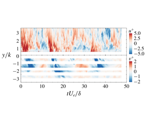
3.3 Indirect evidence of amplitude modulation

This section explores the connection between the small-scale turbulence near and within the porous beds and large-scale motions overlying the beds in the surface flow, using various statistical approaches and leveraging the high-resolution, low-frame-rate PIV measurements. Based on the instantaneous and statistical results presented in the previous section, the relationship between upwelling and downwelling events (i.e. those events that drive flow into and out of the permeable walls) and the streamwise velocity fluctuations above the permeable walls that demarcate the passage of large-scale structures was evident. Kim et al. (Reference Kim, Blois, Best and Christensen2018) used conditionally averaged velocity fields obtained for a given local vertical flow event at the permeable interface to demonstrate that upwelling ($v>0$)/downwelling ($v<0$) events at the wall interface are statistically tied to the simultaneous occurrence of large-scale regions of negative/positive streamwise velocity fluctuations, respectively, in the surface-flow region that are highly reminiscent of large-scale motions in impermeable-wall turbulence. In impermeable, smooth-wall turbulence, Hutchins & Marusic (Reference Hutchins and Marusic2007a) reported that small-scale streamwise velocity fluctuations in the near-wall region are more energetic/quiescent under the influence of positive/negative large-scale streamwise velocity fluctuations in the outer layer. This AM of the near-wall, small scales by larger scales in the outer layer was quantified by Mathis et al. (Reference Mathis, Hutchins and Marusic2009). The behaviour of the wall-normal velocity component at the interface of the permeable walls considered herein, particularly its role in transport across the interface, may also be linked to the same phenomenological relationship. In this regard, the link between velocity quantities at the interface ($u$, the sign of $v$) and the passage of large-scale motions in the surface flow could be indicative of modulation of the small scales near, and within, the permeable walls by outer large-scale motions, similar to that originally found in smooth-wall turbulence (Mathis et al. Reference Mathis, Hutchins and Marusic2009). While the high-frame-rate PIV data will be used to quantify these connected interactions using the AM metrics that were introduced by Mathis et al. (Reference Mathis, Hutchins and Marusic2009) for smooth-wall turbulence, following Efstathiou & Luhar (Reference Efstathiou and Luhar2018), this connection is first explored using unconditional and conditionally averaged profiles of streamwise velocity skewness to infer enhanced/diminished AM effects. Inference of AM effects from velocity skewness was recently suggested, as wall-normal profiles of the AM correlation coefficient proposed by Mathis et al. (Reference Mathis, Hutchins and Marusic2009) show remarkable resemblance to wall-normal profiles of streamwise velocity skewness (Schlatter & Örlü Reference Schlatter and Örlü2010b; Mathis et al. Reference Mathis, Marusic, Hutchins and Sreenivasan2011b). Then, the spatial characteristics of surface–subsurface interactions are explored using conditional averaging of the high-resolution, low-frame-rate PIV data based on the occurrence of upwelling and downwelling events.

3.3.1 Skewness

Following the approach of Efstathiou & Luhar (Reference Efstathiou and Luhar2018), profiles of streamwise velocity skewness ($\text{Skew}_{u}$) are used to infer the presence of AM effects in the permeable smooth- and rough-wall cases. This analysis is restricted to the low-frame-rate PIV data acquired at the trough position of each wall model as this region of each permeable wall embodies flow interactions across the interface. To explore potential AM effects during upwelling and downwelling processes, the velocity fields for each wall model were separated by upwelling (characterized by $v>0$ at the permeable interface) and downwelling ($v<0$) events at the interface. The conditional streamwise velocity skewness, $\text{Skew}_{u}$, was then calculated for upwelling and downwelling events by first ensemble averaging across the conditional ensembles (one for $v>0$ and the other for $v<0$) followed by line averaging in the streamwise direction over a limited region of $3.6<x/k<5.3$ and $3.1<x/k<5.8$ comprising one open pore space along the trough position for the permeable smooth- and rough-wall cases, respectively. The reference point for the conditional event (i.e. discerning between upwelling and downwelling events) was positioned at $x_{ref}=4.4k$ and $y_{ref}=-0.2k$, as indicated by the black markers in figure 5. This procedure appropriately reflects the impact of upwelling and downwelling events on $\text{Skew}_{u}$ across the permeable interface. In addition to these conditionally averaged skewness profiles, the unconditional skewness was also calculated, as was the skewness of the impermeable smooth-wall case, to highlight the effects of permeability.

Figure 6. Wall-normal profiles of unconditional and conditionally averaged streamwise velocity skewness for the permeable (a) smooth- and (b) rough-wall cases. Profiles from the impermeable smooth-wall case and the DNS of Schlatter & Örlü (Reference Schlatter and Örlü2010a) are included for comparison.

Figure 6 presents the unconditional and conditional streamwise velocity skewness profiles for the permeable smooth- and rough-wall cases as well as the impermeable smooth-wall case. As shown in figure 6(a), the impermeable smooth wall $\text{Skew}_{u}$ shows excellent agreement with the direct numerical simulations (DNS) from Schlatter & Örlü (Reference Schlatter and Örlü2010a) at comparable $Re$ ($Re_{\unicode[STIX]{x1D703}}\simeq 2540$), validating the measurement protocol used herein as well as the fidelity of the PIV data. The unconditional skewness profile for the permeable smooth-wall case diverges from the baseline impermeable smooth-wall case below $(y-d)/\unicode[STIX]{x1D6FF}=0.05$, illustrating that permeability increases near-wall streamwise velocity skewness. Leveraging the intrinsic link between $\text{Skew}_{u}$ and AM (Schlatter & Örlü Reference Schlatter and Örlü2010b; Mathis et al. Reference Mathis, Marusic, Hutchins and Sreenivasan2011b), these trends represent further inferential evidence of AM effects in permeable-wall turbulence. In particular, the higher magnitude of unconditional $\text{Skew}_{u}$ for the permeable-wall case compared to the impermeable bed suggests that wall permeability enhances this modulating effect, in a similar fashion to that recently observed for impermeable rough-wall flow (Anderson Reference Anderson2016; Pathikonda & Christensen Reference Pathikonda and Christensen2017).

The conditionally averaged $\text{Skew}_{u}$ profiles for the permeable smooth-wall case diverge from the unconditional one, with the $\text{Skew}_{u}$ associated with downwelling flow (linked to the passage of large-scale regions of $u>0$ in the surface flow) being higher in magnitude and the $\text{Skew}_{u}$ associated with upwelling events being lower in magnitude. This difference persists until $(y-d)/\unicode[STIX]{x1D6FF}\simeq 0.6$, after which the conditional $\text{Skew}_{u}$ profiles collapse with the unconditional profile. In the context of AM, the higher skewness associated with downwelling events, which occur during the passage of large-scale regions of high streamwise momentum in the surface flow, is entirely consistent with that previously reported for impermeable-wall turbulence where the passage of high-momentum events in the outer layer excites small-scale turbulence in the near-wall region (Chung & McKeon Reference Chung and McKeon2010; Hutchins et al. Reference Hutchins, Monty, Ganapathisubramani, Ng and Marusic2011; Pathikonda & Christensen Reference Pathikonda and Christensen2019). Likewise, the lower skewness associated with upwelling events, which occur during the passage of large-scale regions of low streamwise momentum in the surface flow, is consistent with impermeable-wall turbulence where the passage of low-momentum events in the outer layer suppresses small-scale turbulence in the near-wall region. Zhang & Chernyshenko (Reference Zhang and Chernyshenko2016) interpreted AM of the ‘small’ and ‘fast’ scales near the wall by the ‘large’ and ‘slow’ scales in the outer region in a quasi-steady, quasi-homogeneous manner, with the former responding to the latter as a slow variation in instantaneous $Re$. Metzger & Klewicki (Reference Metzger and Klewicki2001) and Mathis et al. (Reference Mathis, Marusic, Hutchins and Sreenivasan2011b) examined the increasing trend displayed by skewness factor with $Re$ and noted that this behaviour is consistent with a similar trend of AM and $Re$. Thus, as the large-scale motions strengthen with increasing $Re$, so do AM effects and skewness. In this regard, the noted deviations between the conditionally averaged $\text{Skew}_{u}$ profiles may be due to variation of the local $Re$ whereby the passage of large-scale regions of high/low streamwise momentum, associated with downwelling/upwelling events at the interface, results in an increase/decrease of the local $Re$.

The permeable rough-wall case (figure 6b) displays a similar behaviour as the permeable smooth-wall case, with downwelling-associated skewness consistently higher than the unconditional and upwelling-associated skewness profiles. Interestingly, unlike the permeable smooth-wall case, where deviation from the impermeable smooth-wall case was noted in the near-wall region, the unconditional skewness for the permeable rough-wall case does not diverge from the baseline smooth impermeable case except in the immediate vicinity of the hemispherical topography where noted peaks are observed in both the unconditional and conditional $\text{Skew}_{u}$ profiles for the permeable rough-wall case.

3.3.2 POD filtered conditional averages

With the clear linkage between the occurrence of upwelling/downwelling events across the permeable interface with the passage of large-scale regions of low/high streamwise momentum in the surface flow, and the coupled diminished/enhanced AM effect under such conditions, the spatial signatures of these processes are considered further. In order to examine the modulating effect of outer large scales on the small scales near and within the permeable interface for the smooth- and rough-wall cases, a scale decomposition based on POD was employed (Berkooz, Holmes & Lumley Reference Berkooz, Holmes and Lumley1993; Adrian, Christensen & Liu Reference Adrian, Christensen and Liu2000a), followed by conditional averaging based on the occurrence of upwelling and downwelling events. To this end, POD was performed on the permeable smooth- and rough-wall cases for a targeted domain of $12k\times 3.5k$ (equivalently $3.4\unicode[STIX]{x1D6FF}\times 1\unicode[STIX]{x1D6FF}$) and $12k\times 5.2k$ ($2.6\unicode[STIX]{x1D6FF}\times 1\unicode[STIX]{x1D6FF}$) in the surface-flow region, respectively. One-thousand uncorrelated velocity fields per wall condition from the low-frame-rate PIV data at the trough position were employed in this analysis.

Figure 7. Contour maps of conditionally averaged large-scale (a,e) streamwise ($u_{L}^{+}$) and (b,f) wall-normal ($v_{L}^{+}$) velocities and small-scale r.m.s. (c,g) streamwise ($u_{rms,S}^{+}$) and (d,h) wall-normal ($v_{rms,S}^{+}$) velocities based on (a–d) upwelling and (e–h) downwelling events for the permeable smooth-wall case. Arrows indicate the sign of the wall-normal velocity events at the interface used to condition the ensembles.

The case of the permeable smooth wall is examined first to isolate the role of wall permeability. Using the relationship between cumulative TKE and POD mode number (not reported herein for brevity), a cutoff filter was set at 60 % of cumulative TKE to decouple the large scales (the first 46 most energetic POD modes) from the small scales (POD modes 47 and up). It should be noted that the analysis presented is rather insensitive to the POD mode cutoff selected to separate the larger and smaller spatial scales. Each instantaneous velocity field in a given conditional ensemble (upwelling/downwelling) was then projected onto the first 46 modes to yield the associated instantaneous, large-scale velocity field. The associated instantaneous, small-scale field was then formed by subtracting this large-scale field from the original one. Conditional averages of the large-scale streamwise and wall-normal velocities and the small-scale streamwise and wall-normal turbulence intensities were computed to explore enhancement/suppression of small-scale turbulence near and within the permeable walls by large-scale motions in the surface flow during downwelling/upwelling events.

Figure 7 presents these conditionally averaged quantities for upwelling and downwelling events for the permeable smooth-wall case. These results confirm that the large-scale streamwise surface flow is always negatively correlated with the large-scale, wall-normal flow at the wall interface, which is consistent with the patterns noted in the instantaneous velocity fields presented in figure 4. Of particular interest, small-scale turbulence activity very close to the wall is excited/suppressed (figures 7g and 7h/7c and 7d) under the action of large-scale regions of positive/negative streamwise velocity fluctuations (figures 7e/7a) associated with downwelling/upwelling (figures 7f/7b) events at the permeable interface. These patterns are entirely consistent with that previously noted in impermeable smooth- and rough-wall turbulence and demonstrate the specific role of the surface-flow large scales in modulating the near-wall small scales linked to upwelling and downwelling motions. Remarkably, just below the wall interface, a similar excitation/suppression of small-scale turbulence persists with the passage of high/low streamwise momentum large scales in the surface flow. This region of enhanced/diminished small-scale turbulence within the permeable smooth wall occurs along the inclined pathway of penetrating flow apparent in the conditionally averaged large-scale wall-normal velocity (figures 7b and 7f) and that identified in figure 5(a). Thus, it appears that AM effects not only occur in the near-surface-flow region, but they also persist within the permeable smooth wall.

Figure 8. As in figure 7, but for the permeable rough-wall case.

Figure 9. (a,b) Schematics illustrating flow penetration paths for the permeable smooth- and rough-wall cases, respectively, as identified in figure 5. (c,d) Time–height contours of fluctuating streamwise velocity, $u^{+}(y,t)$, in the surface flow ($y/k>0$) and fluctuating wall-normal velocity, $v^{+}(y,t)$, in the subsurface flow ($y/k<0$) sampled at the streamwise positions noted with vertical red and blue lines in (a,b) for the surface- and subsurface-flow regions, respectively.

The same approach was applied to the permeable rough-wall case wherein the POD analysis indicated that the first thirty most-energetic modes embodied 60 % of the cumulative energy (in contrast to the first 46 POD modes for the permeable smooth-wall case). Figure 8 presents the conditionally averaged large-scale streamwise and wall-normal velocities as well as the small-scale turbulence intensities for the permeable rough-wall case. As with the permeable smooth-wall case, a negative correlation between the large-scale streamwise surface flow and the vertical transport of fluid across the wall interface is noted. Owing to the presence of topography, the large-scale events appear to be larger and more intense. In addition, the large-scale events associated with upwelling/downwelling events at the interface considerably impact the small-scale energy in the vicinity of, and within, the permeable interface by enhancing small-scale activity in both the streamwise and wall-normal velocity components with respect to the occurrence of the low-/high-speed streamwise surface flow. Finally, the enhanced/diminished small-scale activity within the permeable rough wall occurs along the vertically oriented penetrating flow path apparent in the conditionally averaged large-scale wall-normal velocity (figures 8b and 8f) and identified for this wall model in figure 5(b).

3.4 Direct quantification of amplitude modulation

The results presented in the previous section suggest that pore-penetrating turbulence, which contributes to the exchange processes across the permeable interface, is controlled and modulated by the passage of large-scale motions in the surface flow. In fact, this modulating phenomenon appears to extend into the wall, specifically along the preferential paths of the penetrating flow. This section leverages the high-frame-rate PIV measurements to compute quantitative AM metrics for the permeable smooth- and rough-wall cases and to explore the spatio-temporal signatures of these processes.

As noted earlier, each wall model displayed a different characteristic penetrating flow path across the permeable interface (the permeable smooth wall showed an inclined penetration path while the permeable rough wall displayed a vertically oriented path). These penetrating flow paths (schematically illustrated in figures 9a and 9b for the permeable smooth- and rough-wall cases, respectively) are used to guide the temporal probing of the flow using the high-frame-rate PIV data. Figures 9(c) and 9(d) display time–height contours of fluctuating streamwise (surface-flow region, $y/k>0$) and wall-normal (subsurface-flow region, $y/k<0$) velocity extracted from the high-frame-rate PIV data for the permeable smooth- and rough-wall cases, respectively. These time–height fields were constructed by sampling temporal velocity signals for each flow case at fixed streamwise locations (as denoted with lines in figures 9a and 9b). The pore-flow sampling location was shifted $0.5k$ downstream of the sampling location for the surface flow to capture the dynamics within the penetrating flow patterns described in figure 5. This offset corresponds to $tU_{e}/\unicode[STIX]{x1D6FF}\simeq 0.14$, which is negligible in any variation of the structural characteristics of both the surface and subsurface flows. It should also be noted that, owing to the mask residing along the perimeter of the packing spheres, where excessive optical aberration occurred, the pore flow is only partially presented in figures 9(c) and 9(d).

The time–height fields presented in figures 9(c) and 9(d) confirm the periodic nature of the surface-flow events, which alternate between high and low streamwise momentum, and reveal that this periodicity also occurs within the subsurface flow. In particular, they clearly illustrate that downwelling flow events ($v<0$) in the subsurface-flow region, transporting fluid deep into the porous domain, occur simultaneously with large-scale regions of high streamwise momentum ($u>0$) in the surface flow. The opposite occurs during subsurface upwelling events ($v>0$) that transport pore-scale fluid towards the interface, for which large-scale regions of low streamwise momentum ($u<0$) occur simultaneously in the surface flow. These plots represent a direct way to visualize these temporal connections and provide additional evidence that substantiates the hypothesis that modulation of the small scales occurs not only in the near-wall region but also within the permeable walls. These time–height contours also reveal that the temporal interactions between the surface and subsurface flows are very different for the permeable smooth- and rough-wall cases. For the permeable rough-wall case (figure 9d), the subsurface flow is characterized by periodic and larger-scale coherent motions that penetrate deep into the porous bed and appear to be in-phase with the surface flow. In contrast, flow over the smooth permeable wall (figure 9c) exhibits significantly reduced penetration depth and flow coherence, although the subsurface vertical motions remain in-phase with the surface flow. This observation highlights the apparent role of surface topography in inducing more intense and more regularized transport of momentum and energy across the permeable interface.

The inner–outer interactions between the large scales in the surface flow and the smaller scales near the wall interface, as well as within the subsurface, can be quantified using various correlation metrics as introduced and discussed by Mathis et al. (Reference Mathis, Hutchins and Marusic2009), Schlatter & Örlü (Reference Schlatter and Örlü2010b), Bernardini & Pirozzoli (Reference Bernardini and Pirozzoli2011) and Eitel-Amor, Örlü & Schlatter (Reference Eitel-Amor, Örlü and Schlatter2014) for wall-bounded turbulence. Mathis et al. (Reference Mathis, Hutchins and Marusic2009), based on time series of streamwise velocity acquired at fixed wall-normal positions in the inner and log regions of the turbulent boundary layer, proposed the correlation

(3.3)$$\begin{eqnarray}R^{AM}(y_{2};y_{1})=\frac{\overline{u_{L}(y_{1})E_{L}[u_{s}(y_{2})]}}{\unicode[STIX]{x1D70E}_{u_{L}}(y_{1})\unicode[STIX]{x1D70E}_{E_{L}[u_{s}]}(y_{2})},\end{eqnarray}$$

between the large-scale streamwise velocity $u_{L}(y_{1})$ (separated from the smaller scales, $u_{s}(y_{2})$ via a low-pass filter with a cutoff wavelength comparable to $\unicode[STIX]{x1D6FF}$) and the large-scale envelope of the small-scale streamwise velocity $E_{L}[u_{s}(y_{2})]$ determined using a Hilbert transform [where $\unicode[STIX]{x1D70E}_{(\cdot )}$ denotes the r.m.s. of $(\cdot )$]. Mathis et al. (Reference Mathis, Hutchins and Marusic2009) reported two versions of this correlation: $R^{AM}(y_{2};y_{1}=y_{2})$, which samples the large scales at the same wall-normal position as the small scales (single-point analysis), and $R^{AM}(y_{2};y_{1})$, where the large scales are sampled at a fixed wall-normal position in the outer region, $y_{1}$, while the small scales are sampled at all wall-normal positions (two-point analysis). More recently, leveraging whole-field velocity data afforded by computations, Bernardini & Pirozzoli (Reference Bernardini and Pirozzoli2011), Eitel-Amor et al. (Reference Eitel-Amor, Örlü and Schlatter2014) and Dogan et al. (Reference Dogan, Örlü, Gatti, Vinuesa and Schlatter2019) reported full two-dimensional cross-correlations of the form

(3.4)$$\begin{eqnarray}R_{\boldsymbol{u}}(y_{1},y_{2})=\frac{\overline{u_{L}(y_{1})E_{L}[\boldsymbol{u}_{s}(y_{2})]}}{\unicode[STIX]{x1D70E}_{u_{L}}(y_{1})\unicode[STIX]{x1D70E}_{E_{L}[\boldsymbol{u}_{s}]}(y_{2})},\end{eqnarray}$$

and

(3.5)$$\begin{eqnarray}C_{\boldsymbol{u}}(y_{1},y_{2})=\frac{\overline{u_{L}(y_{1})\boldsymbol{u}_{s}^{2}(y_{2})}}{\unicode[STIX]{x1D70E}_{u_{L}}(y_{1})\unicode[STIX]{x1D70E}_{\boldsymbol{u}_{s}}^{2}(y_{2})},\end{eqnarray}$$

respectively, where $\boldsymbol{u}=(u,v)$ (the two velocity components resolved in the PIV measurements presented herein), with the latter suggested as an alternative (Schlatter & Örlü Reference Schlatter and Örlü2010b), yet complementary (Mathis et al. Reference Mathis, Marusic, Hutchins and Sreenivasan2011b), AM metric based on the relationship between skewness and amplitude modulation in wall turbulence. It should be noted that $R^{AM}$ of Mathis et al. (Reference Mathis, Hutchins and Marusic2009) is a subset of the fully two-dimensional $R(y_{1},y_{2})$, with the single-point version of $R^{AM}$ being the diagonal of $R$ with $y_{1}=y_{2}$, while the two-point version of $R^{AM}$ represents a profile across $R$ for $y_{1}=\text{const}$. In the current work, the high-frame-rate planar PIV data acquired simultaneously in the streamwise–wall-normal plane of both the surface and subsurface flows for both permeable smooth- and rough-wall flow are leveraged to compute both $R$ and $C$ within the $y_{1}{-}y_{2}$ plane for the streamwise and wall-normal velocity components. Although previous studies have suggested that scale separation via filtering in the spanwise direction is most effective, particularly at low and moderate $Re$ (Bernardini & Pirozzoli Reference Bernardini and Pirozzoli2011; Eitel-Amor et al. Reference Eitel-Amor, Örlü and Schlatter2014; Dogan et al. Reference Dogan, Örlü, Gatti, Vinuesa and Schlatter2019), the current high-frame-rate PIV datasets contain no spatial information in the spanwise direction. Therefore, a temporal filter corresponding to $\unicode[STIX]{x1D706}_{c}=\unicode[STIX]{x1D6FF}$ (similar to that employed by Mathis et al. (Reference Mathis, Hutchins and Marusic2009)) is used herein to separate the larger and smaller scales in the streamwise and wall-normal velocity components in the surface-flow region.

Figure 10. Correlation coefficients (a,c,e) $R_{u}(y_{1},y_{2})$ and (b,d,f) $R_{v}(y_{1},y_{2})$ for the permeable (a,b) smooth- and (c,d) rough-wall cases, contrasted with that for (e,f) impermeable smooth-wall flow reproduced from Pathikonda & Christensen (Reference Pathikonda and Christensen2019).

Figure 11. Correlation coefficients (a,c) $C_{u}(y_{1},y_{2})$ and (b,d) $C_{v}(y_{1},y_{2})$ for the permeable (a,b) smooth- and (c,d) rough-wall cases.

The degree of interaction between the outer larger scales and the smaller scales close to the smooth and rough permeable interfaces is first considered in figure 10 from the perspective of $R_{u}$ and $R_{v}$, given by (3.4), for the permeable smooth- and rough-wall cases. These permeable-wall results are contrasted with the same in figures 10(e) and 10(f) for the baseline case of impermeable smooth-wall flow at $Re_{\unicode[STIX]{x1D70F}}=1410$ from Pathikonda & Christensen (Reference Pathikonda and Christensen2019), computed from similar high-frame-rate PIV measurements in the same flow facility and with the same filtering methodology utilized herein. As discussed in Bernardini & Pirozzoli (Reference Bernardini and Pirozzoli2011), the imprint of inner–outer interactions can be discerned in this two-dimensional correlation coefficient via strong, off-diagonal, positive correlation values for $y_{1}>y_{2}$. All three cases presented in figure 10 embody this imprint of AM effects in both the streamwise and wall-normal velocity components, highlighting the clear presence of amplitude modulation of the near-wall smaller scales by the outer, larger scales. Of note, the magnitude of this correlation for $y_{1}>y_{2}$ is larger in both permeable-wall cases compared to the baseline impermeable-wall flow in both $R_{u}$ and $R_{v}$, meaning that the large-scale motions overlying these permeable walls have a stronger modulating effect on the small-scale turbulence very close to both permeable interfaces, as compared to the baseline impermeable-wall flow. This distinction suggests that wall permeability enhances the AM phenomenon, as inferred earlier from indirect measures of the same effect (streamwise velocity skewness and conditional averaging). The permeable rough-wall results, particularly for $R_{u}$, suggest that the coupling of permeability with surface topography further increases the AM effect, likely because the large-scale motions along the trough position exhibit enhanced coherence due to the effects of roughness-formed channelling (Kim et al. Reference Kim, Blois, Best and Christensen2018, Reference Kim, Blois, Best and Christensen2019). An additional source for this enhancement could be the more regular shedding of smaller-scale structures from the hemispherical roughness elements of the permeable rough wall. Thus, the enhanced coherence of the large-scale motions and additional small scales shed from the permeable rough wall may be responsible for inducing a stronger AM effect as compared to the permeable smooth-wall case.

A similar trend is noted in figure 11 which presents $C_{u}$ and $C_{v}$, given by (3.5), for the permeable smooth- and rough-wall cases (Pathikonda & Christensen (Reference Pathikonda and Christensen2019) did not report $C$ for impermeable smooth-wall flow). As discussed in Eitel-Amor et al. (Reference Eitel-Amor, Örlü and Schlatter2014) and Dogan et al. (Reference Dogan, Örlü, Gatti, Vinuesa and Schlatter2019), this two-dimensional correlation coefficient in the $y_{1}{-}y_{2}$ plane also reveals the presence of AM effects via strong, off-diagonal, positive correlation values for $y_{1}>y_{2}$. In contrast to $R$, $C$ leverages the link between the skewness and AM effects as previously reported by Schlatter & Örlü (Reference Schlatter and Örlü2010b) and Mathis et al. (Reference Mathis, Marusic, Hutchins and Sreenivasan2011b), whereby the overall skewness can be reconstructed from various combinations of $u_{L}$ and $u_{s}$, with the specific cross-correlation term between $u_{L}$ and $u_{s}^{2}$ providing an alternative diagnostic for identifying AM of the near-wall smaller scales by the outer, larger scales. Here we extend this concept to both the streamwise and wall-normal velocity components through $C_{u}$ and $C_{v}$, similar to that reported in Blackman & Perret (Reference Blackman and Perret2016) for a turbulent boundary layer overlying an array of cubes. Both the permeable smooth- and rough-wall cases show strong, off-diagonal, positive correlation magnitudes for $y_{1}>y_{2}$, reflecting the noted influence of the outer larger scales on the smaller scales near the permeable interface. As was observed in $R$, the permeable rough-wall $C_{u}$ and $C_{v}$ metrics show higher correlation magnitudes, indicating that these inner–outer interactions are stronger in the presence of topography for flow over a permeable interface.

With the existence of AM effects clearly established in the region just above the smooth and rough permeable walls, the possibility of AM effects penetrating within the permeable walls is considered. To do so, space–time correlations between the large scales in the surface flow and the small scales in the subsurface-flow region were computed. In this case, the large scales were sampled at fixed outer locations of $(y-d)/\unicode[STIX]{x1D6FF}=0.06$ and 0.05 for the permeable smooth- and rough-wall cases (horizontal dashed lines in figures 9c and 9d), respectively, while the temporal signals of the pore flow were acquired along the vertical blue lines illustrated in figures 9(a) and 9(b). A different spectral filter size was required to properly decompose the large and small scales in the subsurface flow. The present subsurface flow travelling along the trough side is dominated by a channelling effect with a periodic acceleration and deceleration at each pore (Horton & Pokrajac Reference Horton and Pokrajac2009; Manes et al. Reference Manes, Pokrajac, McEwan and Nikora2009; Kim et al. Reference Kim, Blois, Best and Christensen2018). Thus, the dominant length scale of the subsurface flow is smaller than that of the surface flow, so a quarter of the boundary-layer thickness, which is approximately half the size of the packing sphere diameter, was used as the cutoff wavelength ($\unicode[STIX]{x1D706}_{c}=0.25\unicode[STIX]{x1D6FF}$) in the spectral filter, whereas the filter size for the large-scale surface flow remained identical ($\unicode[STIX]{x1D706}_{c}=\unicode[STIX]{x1D6FF}$).

Figure 12. AM correlation maps between the small-scale (a,b) streamwise and (c,d) wall-normal subsurface velocities and the large-scale surface flows for the permeable (a,c) smooth- and (b,d) rough-wall cases. Black dashed line demarcates $R=0.3$ iso-contour level.

Figure 12 presents AM correlation maps in the space–time domain illustrating AM of the small-scale subsurface flow by the large scales in the surface flow. Remarkably, these results suggest that AM effects extend deep into the subsurface-flow region, as conjectured earlier via indirect measures of this effect. Figure 12 also highlights that, for both permeable walls, the modulation occurs mainly along the penetrating flow paths of upwelling and downwelling flow and progressively vanishes deep into the wall as the small-scale turbulence decays. Further, these results suggest that the interfacial topography plays a role in defining the penetration depth of the AM effect. To highlight this behaviour, an iso-contour line in these correlations is highlighted as a black dashed-line for a value of $R=0.3$. By doing so, two distinct regions of high correlation, separated by a relatively narrow band of lower correlation, are identified. For the permeable smooth-wall case, these regions are labelled $S_{u}^{\prime }/S_{v}^{\prime }$ and $S_{u}^{\prime \prime }/S_{v}^{\prime \prime }$ for the streamwise/wall-normal velocity component (figures 12a and 12c), where $S_{u}^{\prime }$ and $S_{v}^{\prime }$ are located near the interface ($-0.5<y/k<0$), while $S_{u}^{\prime \prime }$ and $S_{v}^{\prime \prime }$ are located deeper in the permeable bed ($-2<y/k<-1.4$). Of note, these two regions of strong correlation occur at different times relative to the passage of a large-scale event in the surface flow at zero time delay. While $S_{u}^{\prime }$ and $S_{v}^{\prime }$ reveal an AM penetration depth of about $0.5{-}0.6k$ that is temporally in-phase with the passage of a large-scale motion in the surface flow at zero time lag ($\unicode[STIX]{x1D70F}U_{e}/\unicode[STIX]{x1D6FF}=0$), $S_{u}^{\prime \prime }$ and $S_{v}^{\prime \prime }$ are positioned at $\unicode[STIX]{x1D70F}U_{e}/\unicode[STIX]{x1D6FF}=-1.6$, suggesting that the flow at $y/k\simeq -1.5$ is only weakly correlated to the penetrating flow at $\unicode[STIX]{x1D70F}U_{e}/\unicode[STIX]{x1D6FF}=0$, but more strongly correlated to the penetrating flow occurring earlier in time at an upstream location. The permeable rough-wall correlations (figures 12b and 12d) exhibit several fundamental differences with their smooth-wall counterparts. First, the primary high-correlation regions, $R_{u}^{\prime }$$R_{v}^{\prime }$, are notably larger and extend deeper into the bed ($-1<y/k<0$), revealing an AM penetration depth of approximately $k$. Moreover, the secondary correlations, $R_{u}^{\prime \prime }$ and $R_{v}^{\prime \prime }$, which are smaller in spatial extent, reside deeper in the bed near $y/k=-2.5$ and are centred at positive time delays. This latter observation suggests that these AM effects occur after the passage of the large-scale motion in the surface flow at zero time delay, meaning that it is correlated to a large-scale event that sits downstream at the time of the subsurface excitation. Thus, these results indicate that, due to enhanced flow penetration induced by surface topography, the permeable rough-wall case exhibits more intense and deeper penetration of AM effects compared to the smooth-wall case.

3.5 Conditional averaging based on zero-crossing events

Due to the rich spatio-temporal information of the surface and subsurface flows embodied in the high-frame-rate PIV measurements, the aforementioned modulating effect can also be explored using conditional averaging of the large- and small-scale spatial signatures captured within the PIV FOVs. The conditional event utilized herein is given by zero crossings of the large-scale velocity fluctuations in a space–time domain. Unlike the conditional averaging by POD (figure 7) or the AM correlation coefficients (figures 10, 11 and 12), the advantage of the zero-crossing conditional event in this study is that it simultaneously reveals the spatial characteristics of the modulating effect along with its temporal evolution.

The concept of this conditional averaging approach was first employed by Baars et al. (Reference Baars, Talluru, Hutchins and Marusic2015) to decompose the large- and small-scale fluctuating energies for wall-bounded turbulence. Although this work was based on point measurements by leveraging Taylor’s hypothesis, unique features for the modulating phenomenon were successfully revealed. A similar approach was also used with LES data of turbulent channel flow to reconstruct large-scale coherent regions interacting with small-scale turbulence (Chung & McKeon Reference Chung and McKeon2010). Recently, the zero-crossing conditional averaging was extended to high-frame-rate PIV data by Pathikonda & Christensen (Reference Pathikonda and Christensen2019) to capture directly the spatio-temporal signature of the large- and small-scale interactions (without the need for Taylor’s hypothesis reconstruction) in a smooth-wall TBL. In the present work, a similar approach was utilized to give a clear picture of AM effects in a space–time domain for the flow overlying the two permeable walls.

Time series of large-scale streamwise velocity, $u_{L}$, were used to define the events for conditional averaging and were extracted at the same sampling point, $\boldsymbol{x}_{ref}=(x_{ref},y_{ref})$, as that used in the calculation of the AM correlation coefficients. The spectral cutoff filter ($\unicode[STIX]{x1D706}_{c}=\unicode[STIX]{x1D6FF}$) was applied to obtain the large scales from the given time series at the reference point. Following Pathikonda & Christensen (Reference Pathikonda and Christensen2019), positive zero crossings in $u_{L}$ were utilized as the conditional event for this analysis. Following Pathikonda & Christensen (Reference Pathikonda and Christensen2019), identifying the temporal instances $\unicode[STIX]{x1D70F}_{ref^{+}}^{i}$ (where $i$ refers to the $i$th identified zero-crossing event, the ‘+’ denotes the positive zero crossing and $\unicode[STIX]{x1D70F}=tU_{e}/\unicode[STIX]{x1D6FF}$ herein) as the $u_{L}$ crosses from negative to positive in the absolute time ($t$), the conditional events are given by

(3.6)$$\begin{eqnarray}u_{L}(\unicode[STIX]{x1D70F}_{ref^{+}})\equiv u_{L}(x_{ref},y_{ref},\unicode[STIX]{x1D70F}_{ref^{+}})=0,\end{eqnarray}$$

and

(3.7)$$\begin{eqnarray}\frac{\text{d}u_{L}}{\text{d}t}(x_{ref},y_{ref},\unicode[STIX]{x1D70F}_{ref^{+}})>0.\end{eqnarray}$$

The velocity fields associated with these zero-crossing events in both the sFOV and pFOV were formed by collecting the velocity fields as

(3.8)$$\begin{eqnarray}[\boldsymbol{u}|_{+}(x,y,\unicode[STIX]{x1D70F})]^{i}=[\boldsymbol{u}(x,y,\unicode[STIX]{x1D70F}_{ref^{+}}+\unicode[STIX]{x1D70F})]^{i},\end{eqnarray}$$

where $[\cdot ]^{i}$ denotes an ensemble. The $[\boldsymbol{u}|_{+}(x,y,\unicode[STIX]{x1D70F})]$ ensembles were formed around the positive zero crossing at $\unicode[STIX]{x1D70F}_{ref^{+}}$ over an interval $\pm 2.5\unicode[STIX]{x1D70F}$ (where $\unicode[STIX]{x1D70F}=tU_{e}/\unicode[STIX]{x1D6FF}$). Applying this process to the permeable smooth- and rough-wall datasets yielded 323 and 279 positive zero-crossing events, respectively, and these ensembles were employed in the conditional averages at each $\unicode[STIX]{x1D70F}$.

Figure 13. Representative time series of large-scale (a) streamwise ($u_{L}^{+}$) and (b) wall-normal ($v_{L}^{+}$) velocity extracted at $y_{ref}/\unicode[STIX]{x1D6FF}\simeq 0.06$ for the permeable smooth-wall case. All identified positive zero-crossing points ($\unicode[STIX]{x1D70F}_{ref^{+}}$; red circles) and three example neighbourhoods of width $\pm 2.5\unicode[STIX]{x1D70F}$ (where $\unicode[STIX]{x1D70F}=tU_{e}/\unicode[STIX]{x1D6FF}$) (red lines) are identified.

Figures 13(a) and 13(b) present representative time series of large-scale streamwise and wall-normal velocity fluctuations, respectively, from the permeable smooth-wall case, acquired at the aforementioned reference point $(x_{ref},y_{ref})$. Of all positive $u_{L}$ zero crossings demarcated by the red circles in figure 13(a), three examples are highlighted with solid red lines demarcating the temporal neighbourhoods [$-2.5tU_{e}/\unicode[STIX]{x1D6FF}$, $2.5tU_{e}/\unicode[STIX]{x1D6FF}$] around each positive zero crossing. Each identified $u_{L}$ event embodies a local minimum and local maximum that correlates well with a local upwelling (local maximum in $v_{L}^{+}$) and local downwelling (local minimum in $v_{L}^{+}$) event in the time series of $v_{L}$ (figure 13b). Thus, this conditional averaging approach resolves a characteristic signature of the penetrating flow across the wall interface, allowing a better understanding of the spatial structure of the transporting fluid and its resulting influence on the near-wall and subsurface small-scale turbulence in the transitional layer of the permeable walls. As discussed in Pathikonda & Christensen (Reference Pathikonda and Christensen2019), there are instances when identified positive zero-crossing neighbourhoods overlap. Such occurrences were rather rare (∼5 %) and occurred in two neighbourhoods at most. Thus, no exceptions were made for these instances. Finally, while positive zero crossings are utilized herein to identify large-scale conditional events for averaging, this analysis could be performed using negative zero crossings in $u_{L}$, which yields an equivalent result simply shifted in time relative to the positive zero-crossing result (Pathikonda & Christensen Reference Pathikonda and Christensen2019).

To explore the temporal variation of small-scale turbulent kinetic energy immediately above and within the permeable walls under the influence of the large scales in the surface flow via conditional averaging, the small-scale velocity field at each instance was decoupled and the corresponding TKE variables were formed as

(3.9)$$\begin{eqnarray}\displaystyle & \displaystyle \langle \boldsymbol{u}|_{+}\rangle _{L}=\langle \boldsymbol{u}|_{+}\rangle ^{i}, & \displaystyle\end{eqnarray}$$

(3.10)$$\begin{eqnarray}\displaystyle & \displaystyle [\boldsymbol{u}|_{+}]_{s}^{i}=[\boldsymbol{u}|_{+}]^{i}-\langle \boldsymbol{u}|_{+}\rangle _{L}, & \displaystyle\end{eqnarray}$$

(3.11)$$\begin{eqnarray}\displaystyle & \displaystyle \langle \text{TKE}|_{+}\rangle _{s}^{i}={\textstyle \frac{1}{2}}\langle \boldsymbol{u}|_{+}^{2}\rangle _{s}^{i}, & \displaystyle\end{eqnarray}$$

and

(3.12)$$\begin{eqnarray}\unicode[STIX]{x1D6E5}\langle \text{TKE}|_{+}\rangle _{s}^{i}=\langle \text{TKE}|_{+}\rangle _{s}^{i}-\langle \text{TKE}|_{+}\rangle _{s,\unicode[STIX]{x1D70F}}^{i},\end{eqnarray}$$

where $\langle \cdot \rangle ^{i}$ indicates an ensemble average over all temporal instances and $\langle \cdot \rangle _{\unicode[STIX]{x1D70F}}^{i}$ refers to ensemble averaging and time averaging to obtain unconditional quantities. Here, TKE denotes a surrogate TKE formed from $u$ and $v$ owing to the planar, two-component velocity data acquired in the $x{-}y$ plane. The small-scale TKE discrepancy, $\unicode[STIX]{x1D6E5}\langle \text{TKE}|_{+}\rangle _{s}^{i}$, is also considered herein to better highlight the variation in the small-scale TKE relative to its unconditional ensemble average. Thus, this TKE discrepancy is a spatio-temporal measure of the energy surplus or deficit from the nominal TKE value depending on enhancement/suppression via AM effects by the passage of high/low streamwise momentum events in the surface flow.

Figure 14. Contour maps of (a–c) large-scale streamwise, $\langle u|_{+}\rangle$, (above the wall) and wall-normal $\langle v|_{+}\rangle$ (below the wall) velocity, (d–f) small-scale TKE, $\langle \text{TKE}|_{+}\rangle _{s}$ (above and within the wall) and (g–i) small-scale TKE discrepancy, $\unicode[STIX]{x1D6E5}\langle \text{TKE}|_{+}\rangle _{s}$ (zoomed in around the permeable interface) for the permeable smooth-wall case at three temporal instances: $\unicode[STIX]{x1D70F}=-0.76$, 0, and 0.76. The dashed lines demarcate the solid structure in the measurement plane at the trough position.

Figure 15. As in figure 14, but for the permeable rough-wall case at three temporal instances: $\unicode[STIX]{x1D70F}=-1.12$, 0 and $1.12$.

The temporal evolution of $\langle u|_{+}\rangle _{L}$ (above the wall) and $\langle v|_{+}\rangle _{L}$ (within the wall) as well as $\langle \text{TKE}|_{+}\rangle _{s}$ and $\unicode[STIX]{x1D6E5}\langle \text{TKE}|_{+}\rangle _{s}$ above and within the permeable smooth and rough walls are shown in figures 14 and 15, respectively, at three temporal instances. These results highlight the mutual interplay between the large-scale surface and subsurface flows and the modulating effect of the large scales upon the small scales in the vicinity of, and within, each permeable wall. The $\langle u|_{+}\rangle _{L}$ contour maps in the surface flow for both wall cases are marked by the passage of large-scale, inclined regions of low ($\langle u|_{+}\rangle _{L}<0$) and high ($\langle u|_{+}\rangle _{L}>0$) streamwise momentum that are spatially correlated with upwelling ($\langle v|_{+}\rangle _{L}>0$) and downwelling ($\langle v|_{+}\rangle _{L}<0$) events across each permeable wall. These patterns are entirely consistent with those identified in the instantaneous velocity fields presented in figure 4 as well as via POD filtering and conditional averaging based on the occurrence of upwelling and downwelling events in figures 7 and 8. However, the results shown in figures 14 and 15 provide more comprehensive spatio-temporal views of these interactions, including how the small-scale TKE just above, and within, the permeable walls evolve with the passage of large-scale structures in the surface flow, particularly during the transition from a large-scale region of low streamwise momentum to a high-momentum region with increasing time. During this transition, large-scale upwelling flow is followed by downwelling flow across the permeable interfaces (evident in $\langle v|_{+}\rangle _{L}$). Under the influence of these large-scale structures in the surface flow, the small-scale TKE, $\langle \text{TKE}|_{+}\rangle _{s}$, is subjected to a modulation effect, revealing suppression (negative $\unicode[STIX]{x1D70F}$) followed by excitation (positive $\unicode[STIX]{x1D70F}$) of small-scale turbulence close to the wall for both permeable cases (figures 14d–f and 15d–f). This excitation/suppression phenomena is quite reminiscent of the POD filtered and conditionally averaged results shown in figures 7 and 8 from the temporally uncorrelated, low-frame-rate PIV data. The corresponding small-scale TKE discrepancy further highlights this modulating effect with respect to the passage of large scales in the surface flow. In particular, a small-scale energy deficit is noted under the influence of a large-scale region of low streamwise momentum (negative $\unicode[STIX]{x1D70F}$) and a small-scale energy surplus is noted with the passage of a high streamwise momentum event (positive $\unicode[STIX]{x1D70F}$), all relative to its mean value for both permeable wall cases. Remarkably, as first identified in the POD filtered conditional averaging results in figures 7 and 8, these plots of small-scale TKE discrepancy in figures 14 and 15 again indicate that the modulating influence of large scales in the surface flow on the small-scale turbulence extends into the permeable walls, with small-scale energy deficit/surplus below the permeable interface with the passage of large-scale low/high streamwise momentum events in the surface flow.

Taken together, these results provide substantial evidence of AM effects in turbulent flow overlying a permeable wall and provide the first direct evidence that these AM effects not only exist in the near-wall region (as has been previously identified in studies of impermeable-wall turbulence) but also extend into the permeable wall through penetrating flow across the permeable interface. The imprint of this modulation effect is more clearly discerned in the permeable rough-wall case, likely because wall permeability accompanied by surface topography induces a more pronounced penetrating flow, allowing more intense vertical exchange of flow between the surface and subsurface regions compared to that of the permeable smooth-wall case.