2.1 Facility

The studied jets exhaust from a convergent nozzle into the $10~\text{m}\times 8~\text{m}\times 8~\text{m}$ anechoic room of the Laboratoire de Mécanique des Fluides et d’Acoustique at École Centrale de Lyon. Compressed dry air is supplied by a centrifugal compressor, which allows continuous operation at a maximum flow rate up to $0.85~\text{kg}~\text{s}^{-1}$ . The maximum nozzle pressure ratio (NPR) is 3.9, corresponding to $M_{j}=1.54$ . The nozzle diameter is $D=38~\text{mm}$ , its nozzle lip is 0.5 mm thick and the contraction ratio is $4.4:1$ (André Reference André2011). Static pressure is measured in the inlet duct 15 diameters upstream of the nozzle, and is combined with ambient pressure measurements and isotropic flow relations to evaluate $M_{j}$ . These flow conditions are monitored to ensure that, once set, $M_{j}$ remains constant within $\pm 0.2\,\%$ . The total temperature is monitored by a K-type thermocouple protruding into the inlet pipe. After a run-time of half an hour, the air supply system is such that the total temperature stabilises at $30\,^{\circ }\text{C}\pm 2\,^{\circ }\text{C}$ depending on day-to-day variation of air temperature at the compressor inlet. The ambient temperature in the anechoic room is also monitored by a thermocouple probe located in a region at rest. Results obtained with two different experimental techniques are reported here: high-speed schlieren visualisations of the jet shear layer and its surroundings, and near-field acoustic measurements. These techniques are applied to 10 jets whose corresponding Mach numbers and characteristics are provided in table 2. The screech Strouhal number $St_{s}$ and the jet Reynolds number $Re_{j}$ are based on the equivalent fully expanded jet velocity $U_{j}$ and density $\unicode[STIX]{x1D70C}_{j}$ . Those setting points are chosen to cover the axisymmetric modes A1 and A2, as well as the flapping mode B. Three setting points relate to the A1 mode. Only one deals with the A2 mode because it tends to coexist with another mode as soon as it moves apart from $M_{j}=1.15$ . Above $M_{j}=1.23$ , a flapping mode is obtained and is studied through six different setting points, which allows one to assess a potential effect of $M_{j}$ on the screech loop characteristics for this given mode. These modes are illustrated in appendix A, on the basis of schlieren visualisations.

2.2 Apparatus

The near-field acoustic measurements are performed using two $1/8$ -inch B&K 4138 microphones, with a Nexus 2692 conditioner. The first reference microphone is mounted fixed to the nozzle rig; the second is mounted on a motorised rig allowing for axial and radial traverses. The same rig is also used to support the conventional $Z$ -type schlieren system set-up built up from two 200 mm f/8 parabolic mirrors spaced by 2.5 m. The light source is a focused high-power Cree XP-L light-emitting diode (LED). Comparative tests on data post-processing specific to this study led to the knife edge being set perpendicular to the jet axis. Axial density gradients are thus observed. The knife edge cut-off is set to approximately 50 %. Grey-scale images are recorded by a Phantom V12 CMOS camera; the grey-level field is denoted by $g(y,z,t)$ . The collecting optics is a Sigma 120–400 mm f/4.5–5.6.

The schlieren films recorded as part of this study arise from two test campaigns. Cases at $M_{j}=1.10$ and $M_{j}=1.35$ were acquired in 2011 by André, Castelain & Bailly (Reference André, Castelain and Bailly2011a ); other cases were acquired in 2016 with identical experimental set-ups. The $M_{j}=1.15$ jet is available from the 2011 and 2016 campaigns, so it can be used for checking consistency. Far-field noise spectra measured in 2011 and 2016 at $130^{\circ }$ with respect to the jet axis are compared in figure 1. The screech frequency and amplitude are found to be in good agreement in the two campaigns. The peak frequency and the sound pressure level of the broadband shock-associated noise also compare very well with each other. The similarity of the hydrodynamic structure of the $M_{j}=1.15$ jets measured in 2011 and in 2016 can also be verified in figure 2 through the juxtaposition of the time-averaged schlieren images. They are also compared in figure 3 by superimposing the profiles along the jet axis of time-averaged grey levels $\overline{g}$ . In these two figures, the grey levels are normalised to get around the different light and camera settings. The distance between the leading edge of the second shock cell and the leading edge of the seventh is found to be 1.3 % longer in 2016 than in 2011. This difference may be attributed to the uncertainties emerging from the calibration of the scaling factor, the precision of the setting points, and possible small modifications of the rig undergone between the two campaigns.

Figure 1. Acoustic spectrum for the $M_{j}=1.15$ jet measured at a distance of 55 $D$ from the nozzle, with an angle of $130^{\circ }$ from the jet axis, in 2011 (——) and 2016 (

).

Figure 2. Time-averaged grey-level field $\bar{g}(y,z)$ of schlieren images of a $M_{j}=1.15$ jet captured in 2011 (top) and in 2016 (bottom).

Figure 3. Normalised profile of $\bar{g}(z)$ (arbitrary units) on the jet axis computed from schlieren images of a $M_{j}=1.15$ jet, in 2011 (——) and 2016 (

).

2.3 Schlieren measurement procedure

Five parameters are taken into account for acquiring the schlieren visualisations. The first one is the spatial extent of the field of view. The second one is the desired sampling rate. These two parameters determine the maximum frame size and the corresponding magnification factor. Finally the exposure time is set by the sampling period and the light intensity. The use of the schlieren visualisation is twofold: to study the turbulent flow in the shear layer and the screech-associated phenomena in the region surrounding the jet. Therefore, two sets of records are available from each campaign. The corresponding camera settings are provided in table 3. One puts priority on the extent of the field of view, and the other prioritises the sampling rate. The minimum acquisition frequency for analysing some flow properties was determined after the work of Veltin, Day & McLaughlin (Reference Veltin, Day and McLaughlin2011), who found satisfactory results by sampling at 15 times the jet characteristic frequency $f_{c}=U_{j}/D_{j}$ , with $U_{j}$ and $D_{j}$ the exit velocity and diameter of the equivalent fully expanded jet. For the worst case, $M_{j}=1.50$ , $f_{c}$ is approximately 10 kHz, so the sampling rate is chosen higher than 150 kHz. This frequency is reached by reducing the size of the frames in the radial direction while keeping a large axial size. Previous studies summarised in table 1 recognised the source of screech to be located between the second and the fifth shock tips. Consequently, the frame used for this study is chosen to contain at least the first five shock cells. However, this measurement is not achievable on one single frame when $M_{j}$ is higher than 1.23 because the spatial extent is limited by the mirror diameter. For these cases, the camera is shifted by an increment of 100 mm ( $2.6D$ ) until the fifth shock cell is filmed. The dataset is thus composed of several films. Schlieren images must be interpreted with some caution because they are altered by integration effects along the optical path. These artefacts are, however, weaker when the flow is characterised by a strong azimuthal and radial coherence, as with screech.

3.1 Overview

A snapshot and time-averaged picture of the schlieren visualisation of the $M_{j}=1.15$ jet are presented in figure 4(a,b). These images clearly show the quasi-periodic pattern of shock cells consisting of compression and expansion waves. The mean spatial period of this pattern is called the shock cell length $L_{sc}$ . The average image shows the decrease of the shock cell intensity with increasing downstream distance from the nozzle. For each pixel, a time signal $g(y,z,t)$ of grey levels acquired at a high sampling rate is available, and the amplitude of its Fourier transform at the screech frequency, denoted by $G_{s}(y,z)$ , is reported in figure 4(c). High values of this coefficient correspond to the darkest regions, and are obtained next to the shock themselves. This high level of fluctuation is attributed to shock oscillation at the screech frequency (Panda Reference Panda1998; André, Castelain & Bailly Reference André, Castelain and Bailly2011b ). Another remark concerns the presence of lobes in the near field that can be linked to the standing-wave pattern observed by Westley & Woolley (Reference Westley and Woolley1969). They interpreted this phenomenon as the resultant effect of the interaction between the instability wave convected with the flow and the screech acoustic waves. More details about the lobed pattern can be observed in figure 5, which represents the axial profiles of grey-level fluctuations at the screech frequency. These profiles are measured at a radial position chosen to display the maximum of instability wave features, and therefore as close as possible to the lip line. However, if the measure is conducted too close to the jet, shocks periodically cross the probed line and sharp discontinuities appear in the profile; therefore the interpretation of those results becomes complicated. A convenient position for the measurement line is found along the line at $y/D=0.55$ for $M_{j}$ lower than 1.32, and along the line at $y/D=0.75$ for higher $M_{j}$ . A look into these profiles shows similarities between all cases. The first observation concerns the lobed shape of the curves, which is similar to the observation in figure 4(c) for the $M_{j}=1.15$ jet. Considering only the midline of the profiles by putting aside the undulations, a second similarity comes out. The wavy pattern is supported by a bell-shaped curve that points out the amplification rate of instability waves. They first grow with increasing distance from the nozzle, then saturate, and finally decay further downstream.

Figure 4. (a) Instantaneous schlieren image $g(y,z,t)$ ( $4~\unicode[STIX]{x03BC}\text{s}$ time exposure). The dashed rectangle shows the field of view of the high-speed records. (b) Averaged field $\overline{g}(y,z)$ . (c) Fluctuating field $G_{s}(y,z)$ at the fundamental screech frequency from schlieren measurement of a jet at $M_{j}=1.15$ , mode A2.

Figure 5. Modulation of the grey-level field $G_{s}$ at the screech frequency (arbitrary scale) along a line at $y/D=0.55$ : (a)  $M_{j}=1.07$ , (b)  $M_{j}=1.10$ , (c)  $M_{j}=1.13$ , (d)  $M_{j}=1.15$ , (e)  $M_{j}=1.23$ , (f)  $M_{j}=1.32$ , (g)  $M_{j}=1.35$ , (h)  $M_{j}=1.37$ , (i)  $M_{j}=1.45$ and (j)  $M_{j}=1.50$ . Shock locations are indicated by vertical dotted lines.

The wavenumber $k_{sw}$ of the lobed pattern was derived by Panda (Reference Panda1999) from the acoustic and hydrodynamic wavenumbers $k_{s}$ and $k_{h}$ , by considering upstream-propagating acoustic and downstream-propagating instability waves. This corresponds to the region upstream of the screech acoustic source, but both waves travel in the same direction downstream of the source. Here we choose to denote by $k_{sw}^{-}$ the wavenumber of the wave pattern where acoustic is retrograde, and $k_{sw}^{+}$ where acoustic is propagative, giving

By convention, all wavenumbers are chosen positive. The corresponding wavelengths $L_{sw}^{-}=2\unicode[STIX]{x03C0}/k_{sw}^{-}$ and $L_{sw}^{+}=2\unicode[STIX]{x03C0}/k_{sw}^{+}$ can be expressed as a function of the screech frequency $f_{s}$ , the convective velocity at screech frequency $U_{c}$ and the speed of sound $c_{0}$ in the jet surrounding: As an illustration, if the convective velocity is approximated to $0.6U_{j}$ , these relations provide $L_{sw}^{-}=0.63D$ and $L_{sw}^{+}=2.68D$ for the case $M_{j}=1.13$ , and $L_{sw}^{-}=1.20D$ and $L_{sw}^{+}=7.26D$ for the case $M_{j}=1.37$ .

The profile of $G_{s}(z)$ for the $M_{j}=1.13$ case shown in figure 5(c) covers the first seven shock cells of the jet. Since the source is expected to be located between the second and the fifth shock tips, the source is somewhere within the profile. The lobes, however, are spaced by a distance similar to $L_{sw}^{-}$ , and there is no clear experimental evidence of a $L_{sw}^{+}$ length scale. More generally, the transition from $L_{sw}^{-}$ to $L_{sw}^{+}$ is not visible for all 10 cases, and the observed wavelength is closer to $L_{sw}^{-}$ than to $L_{sw}^{+}$ .

Nonetheless, the $M_{j}=1.13$ jet presents a notable characteristic that delimits two regions. Upstream of the fourth shock, the lobed pattern wavelength is smaller than the shock cell length, whereas both length scales are equal downstream. The $M_{j}=1.15$ jet exhibits the same features: upstream of a region in between the third and the fourth shocks, the lobes are spaced by a length $L_{sw}^{-}$ smaller than $L_{sc}$ , and these lengths are equal downstream. These jets are the only two having $L_{sw}^{-}$ different from $L_{sc}$ . All other cases present only a single wavelength, which appears to be equal to the shock cell length everywhere. Moreover, the similarity between $L_{sw}^{-}$ and $L_{sc}$ is consistent with Tam’s theoretical conclusions about these length scales. According to Tam et al. (Reference Tam, Seiner and Yu1986, Reference Tam, Parrish and Viswanathan2014), a necessary condition for the screech feedback mechanism to be self-sustained is

By comparison with (3.1a ), $k_{h}-k_{sw}^{-}=-k_{s}$ , Tam’s theory straightforwardly imposes that $L_{sw}^{-}=L_{sc}$ . This statement is not supported by the present experimental results for both $M_{j}=1.13$ and $M_{j}=1.15$ cases. However, the difference between $L_{sw}^{-}$ and $L_{sc}$ is small, although it is clearly observable, which indicates that the condition (3.3) is overly rigid, and the screech conforms with a slightly different condition provided by (3.1a ). The behaviour of the modulation upstream of the source can thus be explained by the theoretical model relying on the wave superposition.

Downstream of the source, the lobes are not spaced by the distance expected from (3.1b ). The period of the pattern seems to be equal to the shock cell length. This feature is likely to result from the modulation of the instability wave by the shock cells, and from the weak amplitude of acoustic waves because of the upstream directivity of screech. The role of shock cells in the existence of the lobed pattern can be demonstrated by considering the jets at $M_{j}=1.07$ , 1.37 and 1.45. For these three Mach numbers, the field of view of the schlieren visualisation is large enough to cover the mixing layer farther downstream from the last detectable shock tip. In each case, the amplitude of lobes starts decaying downstream of the last noticeable shock cell. In addition, the ability of shock cells to modulate the turbulence has been pointed out by André (Reference André2012, in his figure 5.33) throughout particle image velocimetry (PIV) measurements in underexpanded screeching or non-screeching jets. Moreover, the absence of the wavelength $L_{sw}^{+}$ involved in the acoustic–hydrodynamic interaction downstream of the source can be explained by two reasons. Firstly, $k_{h}$ and $k_{s}$ are expected to be close, in particular for the jets at highest Mach numbers, so $k_{sw}^{+}=k_{h}-k_{s}$ is small and may not be noticeable in the spatial extent of the images. Secondly, far-field measurement at the fundamental screech frequency shows a strong upstream directivity (Norum Reference Norum1983; Berland et al. Reference Berland, Bogey and Bailly2007); thus, even in the near field, screech acoustic waves are likely to be weaker downstream of the source.

Finally, the features of the overall profile can be explained as follows. All along the jet, the instability wave is modulated by the shock cell pattern. This phenomenon could explain by itself the presence of lobes spaced by $L_{sc}$ in the near-field map of screech-associated fluctuations, but jets at $M_{j}=1.13$ and $M_{j}=1.15$ are characterised by a modulation wavelength $L_{sw}^{-}$ different from $L_{sc}$ in the first three or four shock cells. This remark suggests that acoustics also plays a role in explaining the lobes where its contribution is strong, but since $L_{sw}^{-}$ is expected to be close to $L_{sc}$ , the difference between them is not perceptible for all other jets. However, downstream of the source, the acoustic contribution is too weak in comparison to the instability wave, preventing any observation of $L_{sw}^{+}$ . If $L_{sc}$ coincides with $L_{sw}^{-}$ in the region upstream of the source, then from (3.1) and (3.3),

This identity will be tested from the analysis of the screech-associated wavenumbers in the next section.

3.2 Wavenumber–frequency spectrum analysis

An attempt is made to experimentally determine the different wavenumbers involved in the screech feedback loop. This is carried out through a one-dimensional spatial Fourier transform applied to Fourier coefficients $G_{s}(z)$ at the screech frequency along the axial direction at $y/D=0.55$ , themselves computed from the high-speed schlieren films. A first analysis is performed in a region located upstream from the source, namely $0\leqslant z\leqslant z_{N}$ , where $z_{N}$ denotes the coordinate of the source location. The determination of this position is detailed in the next section, which benefits from the general overview given in the present section. The source is found either at the third or at the fourth shock tip. As a consequence, the discrete Fourier transform is performed over a short extent that contains only two to four wavelengths depending on the case, so the resolution is low in the wavenumber space. The spatial signal $G_{s}(z)$ used as input to the spatial Fourier transform is weighted by a Gaussian function of width five standard deviations. The wavenumber resolution is improved by doubling the length of the signal by adding zeros. This process is undertaken in order to better distinguish between lobes and randomness, but tests have been performed to ensure that zero padding has no effect on the characterisation of the two main peaks described hereafter.

Figure 6. Wavenumber spectrum at screech frequency $\unicode[STIX]{x1D6F7}_{s}$ (arbitrary linear scale) upstream of the source (——) and downstream (– – –): (a)  $M_{j}=1.07$ , (b)  $M_{j}=1.10$ , (c)  $M_{j}=1.13$ , (d)  $M_{j}=1.15$ , (e)  $M_{j}=1.23$ , (f)  $M_{j}=1.32$ , (g)  $M_{j}=1.35$ , (h)  $M_{j}=1.37$ , (i)  $M_{j}=1.45$ and (j)  $M_{j}=1.50$ . The wavenumber $k_{s}=-\unicode[STIX]{x1D714}_{s}/c_{0}$ is indicated by the vertical dotted line.

The result is shown in figure 6 as a solid line. It consists of a pair of dominant peaks, one characterised by a positive wavenumber and a second characterised by a negative wavenumber. The locations of local maxima are estimated using a method from Gasior & Gonzalez (Reference Gasior and Gonzalez2004) to improve the wavenumber resolution. This method takes advantage of the Gaussian shape of the spectrum calculated from a single-frequency signal windowed by a Gaussian function. The method can be extended to a signal containing more frequencies if their respective Fourier transforms do not overlap. As a consequence, the location of the maximum of a peak can be estimated from the Gaussian function that best fits the peak. The three points on the top of the peaks are used for fitting in this study. Gasior & Gonzalez (Reference Gasior and Gonzalez2004) reported a maximum error of less than $1\,\%$ of the frequency resolution. In the present study the worst resolution is found to be $80~\text{rad}~\text{m}^{-1}$ for the $M_{j}=1.07$ jet without zero padding. An error of less than $1\,\%$ would lead to an error of less than $0.8~\text{rad}~\text{m}^{-1}$ . In order to assess the method, the spatial spectra along all the available radial positions have been computed. The results are found to be weakly dependent on the considered radial position, except for $M_{j}=1.45$ , probably because the distance between the peaks in the wavenumber space is small. In addition, this case exhibits strong shock oscillations that intercept the probed line, causing large discontinuities that produce a significant amount of harmonics. These are likely to influence the determination of the maximum of peaks. The same problem is observed for the $M_{j}=1.50$ jet. In general, the error observed from the lowest peaks is found to be larger, because the effect of overlapping is more significant.

The maxima of the peaks are marked by crosses in figure 6, and are tabulated in table 4. The wavenumber corresponding to the retrograde screech acoustic wave $-k_{s}=-\unicode[STIX]{x1D714}_{s}/c_{0}$ is represented by a dotted line. The comparison between this prediction and the maximum of the peak in the negative wavenumber range shows a good agreement, as also reported in table 4. It provides some confidence to state that this peak is related to the upstream-propagating acoustic wave. As for the peak in positive wavenumbers, it is expected to be $k_{h}=\unicode[STIX]{x1D714}_{s}/U_{c}$ ; the corresponding convective velocity is provided in table 4 normalised by $U_{j}$ , and is indeed roughly equal to $0.6U_{j}$ for all cases. This result is consistent with many studies, for instance those by Powell et al. (Reference Powell, Umeda and Ishii1992), Massey & Ahuja (Reference Massey and Ahuja1997) or Panda & Raman (Reference Panda and Raman1997).

The speed of sound tabulated in table 4 is not equal to the speed of sound of $337~\text{m}~\text{s}^{-1}$ expected from the ambient temperature measured during the experiment. An error of 5 % or less is observed for seven of the 10 cases. A larger error is noticed for the $M_{j}=1.35$ , $1.45$ and $1.50$ jets, in particular for $M_{j}=1.45$ , whose validity has already been examined and called into question. Unfortunately, that dispersion prevents us from providing evidence for the existence or absence of an eventual other type of feedback mentioned by Shen & Tam (Reference Shen and Tam2002), Chatterjee, Ghodake & Singh (Reference Chatterjee, Ghodake and Singh2009) or Edgington-Mitchell, Honnery & Soria (Reference Edgington-Mitchell, Honnery and Soria2015).

Finally, the last column of table 4 compares the wavenumber $k_{sw}^{-}=k_{h}+k_{s}$ associated with the lobed pattern, see (3.1a ), to the shock cell wavenumber averaged over $0\leqslant z\leqslant z_{N}$ . The shock positions are measured from the centreline grey profiles of the averaged schlieren images with an accuracy of $\pm 0.007D$ arising from the width of the shocks, and an additional error of $\pm 0.04z$ from the scaling factor of pixels, but these uncertainties are insignificant in comparison to the margin of error pointed out on $k_{s}$ . The modulation wavenumber is found to be larger than the shock cell wavenumber by a few per cent, except for the case $M_{j}=1.15$ that exhibits $k_{sw}$ 28 % larger than $k_{sc}$ because of the jump in frequency, whereas no change in aerodynamic characteristics of the jet is observed (Clem, Zaman & Fagan Reference Clem, Zaman and Fagan2016). The second largest $k_{sw}^{-}$ in comparison to $k_{sc}$ is found for case $M_{j}=1.13$ : $k_{sw}^{-}$ is 10 % larger than  $k_{sc}$ . The case $M_{j}=1.45$ should not be considered because of the problem of peak overlapping mentioned above. These results are consistent with the conclusions of § 3.1: $k_{h}-k_{s}$ is actually close to $k_{sc}$ , so $L_{sw}^{-}$ is close to $L_{sc}$ , for all but the $M_{j}=1.13$ and $M_{j}=1.15$ cases.

A procedure similar to the one outlined for the region upstream of the source is applied for $z_{N}\leqslant z\leqslant z_{max}$ , where $z_{max}$ is the maximum reachable distance with respect to the schlieren record. The results are plotted as a dashed line in figure 6. The peak in positive wavenumbers is still associated with the instability wave. The corresponding convection velocity is summarised in table 4. Its value is found to be close to $0.7U_{j}$ , hence slightly higher than upstream of the source. A trend of rising convective velocity with axial location was observed by Gojon et al. (Reference Gojon, Bogey and Marsden2015) from a numerical study, and from the same experimental data as the present study but using a different method by Mercier, Castelain & Bailly (Reference Mercier, Castelain and Bailly2016). Regarding the peak in negative wavenumbers denoted by $k_{d}^{-}$ , the distance between this peak and $k_{h}$ is compared to $k_{sc}$ in the last column of table 4, with $k_{sc}$ estimated from the shock cells visible in the range of the spatial spectral analysis. Since the shock cell structure fades out with downstream distance, the estimation of $k_{sc}$ can only be approximate by comparison with the accuracy mentioned for the first few shocks. Nonetheless, the comparison highlights the similarity of these two values in most cases. The $M_{j}=1.45$ case again shows a surprising result in terms of both $k_{h}$ and $(k_{h}+k_{d}^{-})/k_{sc}$ values. In addition to the peak overlapping, the absence of clearly detectable shocks downstream of the fourth one must be pointed out. Thus, comparing $(k_{h}+k_{d}^{-})$ to $k_{sc}$ might not be relevant. For all other cases, the peak in negative wavenumbers $k_{d}^{-}\simeq k_{sc}-k_{h}$ is recognised as the interaction between the shock cell pattern and the instability wave. The corresponding phase velocity $\unicode[STIX]{x1D714}_{s}/k_{d}^{-}$ is subsonic for all cases. No wavenumber peak associated with a retrograde acoustic wave is observed, which is consistent with the determination of the source location $z_{N}$ . No propagative acoustic wave is detected; this is likely to be attributed to the screech directivity, weaker in the jet axis direction with respect to the upstream direction (Norum Reference Norum1983; Berland et al. Reference Berland, Bogey and Bailly2007).

4.1 Radial traverse

In the radial configuration, the reference microphone is fixed at $z=-1.8D$ and $y=1.8D$ considering the centre of the grid as a reference with a precision of $\pm 0.03D$ . The mobile microphone moves along the $y$ direction by steps of 3–5 mm from $y=0.5D$ to $y\simeq 8D$ . The position of the rig is accurately measured at each step. Both microphones are in a region upstream of the jet in which screech is strong, and there is no contribution from the hydrodynamic pressure field; the signals are therefore clean and the phase lag variation along the probed line is expected to be smooth. The relative phase is deduced from the cross-spectrum of the two signals at the screech frequency. It is then unwrapped by adding $2\unicode[STIX]{x03C0}$ at the corresponding jumps, and finally compared with the predicted phase lags. Results for Mach numbers 1.13, 1.15 and 1.35 are presented in figure 7, through the entire spatial range in figure 7(a,c,e), and zoomed in closer to the nozzle in figure 7(b,d,f). The predicted phase lag is superimposed onto experimental results for three different source locations: the third, the fourth and the fifth shock tips.

Figure 7. Comparison between the experimental and the expected phase lag between a reference microphone and a microphone moving along a line perpendicular to the jet axis in the nozzle exit plane. Graphs on the right are the same as graphs on the left but focused close to the nozzle. Curves: ——, fourth shock tip;

, third shock tip;

, fifth shock tip; $\cdots \cdots$ , measurements. Jet Mach number: (a,b)  $M_{j}=1.13$ , (c,d)  $M_{j}=1.15$ , (e,f)  $M_{j}=1.35$ .

Two regions of different behaviour can be observed in these results. For $y/D$ between 0.5 and 4, the phase follows a pattern in fairly good agreement with the results predicted from (4.1). Farther, for $y/D$ between 4 and 8, the phase draws unexpected patterns, particularly for the jets at $M_{j}=1.13$ and 1.35. The choice of the shock corresponding to the screech acoustic source is not straightforward. There is no clear demarcation that would designate unambiguously the source location – the choice might change according to whether the considered region is only $y/D$ between 0.5 and 4, or all the available spatial domain. Nevertheless, the interpretation of the results must be discussed when the distance to the nozzle increases. In fact, the fourth shock is located at $z/D=2.7$ , $2.9$ and $4.8$ for $M_{j}=1.13$ , $1.15$ and $1.35$ respectively. When the moving microphone is at $y/D=4$ , the angle formed between the jet axis and the lines linking the microphone to the source is $124^{\circ }$ , $126^{\circ }$ and $140^{\circ }$ . Norum (Reference Norum1983) investigated the directivity of screech for B and C modes. He observed for the B mode a maximum of screech amplitude at angles close to $170^{\circ }$ , and a drop of 10 dB at an angle of $133^{\circ }$ , and again a 10 dB drop to reach $123^{\circ }$ . These observations were made in the far field, and are therefore not directly applicable in the near field. Nevertheless, measurements of the screech pressure level across the moving microphone path are presented for the case $M_{j}=1.35$ in figure 8. They exhibit the same sharp decrease of amplitude with increasing distance from the nozzle as expected from far-field data. The level is decreased by 20 dB at $y=5.5D$ . The lower the amplitude of the screech acoustic wave, the higher the influence of reflection and other contributions to phase measurement. For this reason, the result of this experiment must be considered with caution when $y$ goes up. After these remarks, the results should not be regarded in the entire domain, and a look back at figure 7(b,d,f) leads us to conclude that the source is located between the third and the fifth shock tips. A better precision in source localisation cannot be obtained with the present method because the displacement of the source does not induce a sufficient phase shift between the two microphones. Better results would be obtained if one of the two microphone phases was less sensitive to the source location. In this configuration, a displacement of the source would involve a larger variation in phase for one microphone than for the other. This is obtainable by placing the reference in the plane perpendicular to the jet axis that passes through the expected source, so $r_{0}$ in (4.1) would be only slightly sensitive to the variation of source location, and $\unicode[STIX]{x0394}\unicode[STIX]{x1D719}$ would mostly be dependent upon $r$ . This method requires a priori knowledge of the result, but this problem is circumvented by moving a microphone along a line parallel to the jet.

Figure 8. Sound pressure level (SPL) measured by the moving microphone SPL normalised by the reference microphone SPL in dB Hz $^{-1}$ at $f_{s}$ , for $M_{j}=1.35$ along the radial traverse in the nozzle exit plane.

4.2 Axial traverse post-processing

In the axial configuration, the reference microphone is fixed at $y=2.4D$ and $z=0.4D$ with the same precision of $\pm 0.03D$ as mentioned for the radial traverse. The moving microphone measures the fluctuating pressure along the $z$ direction by steps of 3–5 mm from $z=-0.1D$ to $z=6D$ or $8D$ . In contrast to the radial traverse, in this configuration the microphone is moved along a line close to the jet, and the fluctuating pressure results from the contribution of the acoustic and of the hydrodynamic pressure fields. The interaction between these two waves modulates the amplitude, the phase velocity and the spatial phase evolution of the resultant wave. This modulation makes it difficult to distinguish the $2\unicode[STIX]{x03C0}$ phase jumps from regular sharp variations in the region where the hydrodynamic pressure field is strong. This is a source of ambiguity for the unwrapping process; the problem is exacerbated because strong hydrodynamic fluctuations are expected to occur near the screech radiation source. For this reason we chose not to use classical methods for phase analysis such as cross-spectrum or cross-correlation, but to extract the screech coherent signal from random fluctuations by performing a phase average analysis. Such an analysis allows for tracking a single phase-averaged wavefront, and as a consequence avoids the $2\unicode[STIX]{x03C0}$ indeterminacy problem.

The phase average is performed for all probed locations along the measurement line. At each location, two synchronous signals are available, one from the reference microphone and the other from the moving microphone. The aim of the first step is to extract the phase at screech frequency provided by the fixed microphone, which will serve as the reference. The signal from the moving microphone will be sorted according to this reference in a second step. To this purpose, the signal measured on the fixed microphone is bandpass-filtered around the screech frequency. The filter is a finite impulse response (FIR) type with cut-off frequency at $\pm 10\,\%$ of $f_{s}$ and a drop of 30 dB at $\pm 30\,\%$ of $f_{s}$ . This filter is applied with a zero-lag method to ensure that the phase of the filtered signal does not become frequency-dependent, so there is no bias in the case of slight drift of the screech frequency. The resulting clean signal is the phase reference, and its maxima delimit the periods of screech. All periods of the record are then discretised into 20 bins of equal length that correspond to 20 increments of phase in a screech period. The samples of the moving microphone record that are in the same bin with respect to a period, and thus in phase, are averaged. This process is repeated for all longitudinal locations of the experiment. A complementary sketch presenting the method is provided in figure 9. In this figure, the phase axis is displayed between 0 and $4\unicode[STIX]{x03C0}$ ; the phase average is performed over two consecutive periods because the wavefront tracking requires that the followed wavefront has enough time to travel from the source to the limits of the measured domain, here $z=0$ and $z=6$ or $8D$ .

Phase-averaged results of all probed locations are in phase with the same reference; the spatial wave can therefore be rebuilt for each phase step. The spatial distribution of the coherent fluctuating pressure $p_{s}$ against the phase with respect to the screech cycle $\unicode[STIX]{x1D719}_{s}$ is provided in figure 10 for the $M_{j}=1.32$ jet. The zero crossing points of the coherent fluctuating pressures are marked by squares or triangles depending on whether they correspond to a rising or a falling edge. These zero crossing points form a pattern which depicts curved lines representing the wavefronts of screech-associated waves. The direction of propagation of these waves is reversed near $z=5D$ . Considering the rising and the falling edges, four wavefronts can be observed in each direction. Both upstream and downstream of the slope inversion position, one of the wavefronts is found to be continuous from the source to the limits of the domain, and is selected to be compared with the expected phase variation $\unicode[STIX]{x0394}\unicode[STIX]{x1D719}$ calculated from (4.1).

Figure 9. Example of phase average process. On the left: ——, reference bandpass filtered signal; $\cdots \cdots$ , moving microphone signal; $\mid$ , period marks. On the right: $\cdots \cdots$ , data from the moving microphone sorted with respect to their phases; ——, phase-averaged signal.

Figure 10. Coherent fluctuating pressure along a line at $y=1.5D$ against the phase with respect to screech cycle in the jet $M_{j}=1.32$ near field. The locations of the wavefronts are reported for the 40 phase steps: ▫, rising edges; ◃, falling edges.

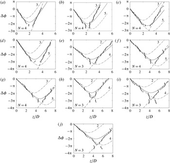
Figure 11. Comparison between the experimental and the expected phase lag between a reference microphone and the microphone moving parallel to the jet at (a–f)  $y=1.5D$ and (g–j)  $y=2D$ : $\cdots \cdots$ ,  $\unicode[STIX]{x0394}\unicode[STIX]{x1D719}$ ; 

  $\text{d}\unicode[STIX]{x1D719}_{s}/\text{d}z=2\unicode[STIX]{x03C0}f_{s}/(0.7U_{j})$ ; ——, the expected result for the source at the shock $N$ ; and $-\cdot -$ , at the labelled shock. Jet Mach number: (a)  $M_{j}=1.07$ , (b)  $M_{j}=1.10$ , (c)  $M_{j}=1.13$ , (d)  $M_{j}=1.15$ , (e)  $M_{j}=1.23$ , (f)  $M_{j}=1.32$ , (g)  $M_{j}=1.35$ , (h)  $M_{j}=1.37$ , (i)  $M_{j}=1.45$ and (j)  $M_{j}=1.50$ .

4.3 Experimental results on source location

The spatial phase evolution of the screech phenomenon is studied across an axially oriented measurement line. This survey aims at investigating the axial evolution of the phase lag. It concerns all the cases defined in table 2. The experimental results are compared with the corresponding expected phase lag in figure 11. A first look at this figure shows that the experimental results exhibit a slope sign inversion at a certain location as well as the expected phase lag. The slope $\text{d}\unicode[STIX]{x1D719}_{s}/\text{d}z$ is inversely proportional to the phase velocity of the wave projected onto the line along which the microphone is moved. The inversion of the sign of the slope translates to the inversion of the direction of wave propagation. In the present study, upstream of the location of slope inversion, the wave propagates upstream and conversely downstream. The study of the slopes of the upstream and downstream branches of the phase evolution provides information about their nature.

Considering only the upstream branch, the measured and the expected phase variations are similar. It is then concluded that the wavenumber of the measured phenomenon is the same as used in the model given in (4.1), $k_{s}$ , for a speed of sound $c_{0}=337~\text{m}~\text{s}^{-1}$ . The wave detected in this region corresponds to the screech acoustic wave.

The measurement across the downstream branch diverges from the prediction. This divergence comes from a difference of slope, that is, a different speed of propagation. The slope of the measured axial phase evolution is higher than the predicted slope for an acoustic wave; the phase velocity of the phenomenon is thus lower than the speed of sound. The near-field pressure at the screech frequency is composed of acoustic and hydrodynamic contributions. The hydrodynamic convective velocity is subsonic for all the cases and is therefore eligible for explaining the slope of the downstream branch. This is also consistent with the conclusion of § 3 stating the absence of acoustic signature downstream of a given region. The slope of the measured phase evolution is compared to the expected slope considering a convective velocity $U_{c}=0.7U_{j}$ , which corresponds to estimation from the wavenumber analysis in § 3. This slope is

The hydrodynamic pressure field is attached to the coherent structures that travel inside the mixing layer almost parallel to the jet axis, and to the line of measurements; thereby, there is no effect of projection. The hydrodynamic phase velocity measured by the microphone traverse is directly equal to the convective velocity. A line of slope corresponding to $U_{c}=0.7U_{j}$ is added as a grey dashed line in figure 11. This line fits the experimental results well, demonstrating that the downstream-propagating branch is dominated by hydrodynamic near-field pressure. The instability wave at the screech frequency is recognised in § 3.1 to be strongly modulated by shock cells, resulting in nodes and antinodes of its amplitude. Thus, the relative acoustic and hydrodynamic amplitudes are dependent upon $z$ . For a given acoustic pressure level, hydrodynamics might dominate at antinodes of the instability wave, and might be dominated by acoustics at nodes. Upstream of the source, the slope of acoustic associated phase lag is negative, and turns positive downstream of the source. The slope of hydrodynamic associated phase lag is positive everywhere. Therefore, wherever the slope is negative, the acoustic pressure field dominates, and the source is necessarily located downstream. This observation sets an upstream limit for the source location, but the downstream limit is still not defined. The source is assumed to be located at a distance of one shock cell or more downstream from the position where the negative slope turns positive. Then, between the inversion location and the source, the positive slope would be sustained by the dominance of the hydrodynamic contribution. Yet, since this contribution is modulated with a wavelength of one shock cell, acoustic should become stronger than hydrodynamic at a certain location upstream of the next shock, so the slope would turn negative again, in contradiction with our first hypothesis. Therefore, the source must be located somewhere in between the last place of negative slope and one shock cell downstream. Constraining the screech source to be located at a shock tip, the shock tip number $N$ corresponding to the source is selected for being the first shock downstream of the last negative slope location. The expected phase lags obtained from the previous and the next shock tips are also included in figure 11 in order to show that there is no ambiguity in finding which agrees better. The fourth shock is found to be the source for all cases except $M_{j}=1.23$ , 1.37, 1.45 and 1.50. The source is the third shock tip for these four cases. The source locations and the associated shock tips are summarised for all cases in table 5. Since acoustic sources are identified, the screech loop is delimited in space, and can be examined in a suitable domain as discussed in § 3.