


1. Introduction
The lateral exchange between a fast moving current and a slower recirculating flow on the side is often encountered in the design of man-made waterways and in the training of natural rivers (Shields, Cooper & Knight Reference Shields, Cooper and Knight1995; Uijttewaal, Lehmann & van Mazijk Reference Uijttewaal, Lehmann and van Mazijk2001). The sedimentation and vegetation in the low-flow areas along the shore are affected by turbulence and waves. Many laboratory experiments were conducted to study the exchanges between the mainstream and the recirculating flow on the side. Most of the existing studies were for sub-critical flow with the value of the Froude number well below unity (Alavian & Chu Reference Alavian and Chu1985; Babarutsi, Ganoulis & Chu Reference Babarutsi, Ganoulis and Chu1989; Booij Reference Booij1989; Uijttewaal Reference Uijttewaal2005; Van Prooijen, Battjes & Uijttewaal Reference Van Prooijen, Battjes and Uijttewaal2005; Xiang et al. Reference Xiang, Yang, Wu, Gao, Li and Li2020; Yossef & de Vriend Reference Yossef and de Vriend2010). Numerical simulations have also been conducted for sub-critical flow of low Froude number using the rigid-lid approximation (McCoy, Constantinescu & Weber Reference McCoy, Constantinescu and Weber2008; Xiang et al. Reference Xiang, Yang, Wu, Gao, Li and Li2020). However, the flow in rivers is often super-critical during flooding events (Petaccia et al. Reference Petaccia, Natale, Savi, Velickovic, Zech and Soares-Fraz ao2013; Kvočka, Ahmadian & Falconer Reference Kvočka, Ahmadian and Falconer2017). These super-critical flows with large Froude numbers are not describable by the conventional theory of turbulence. The waves have a prominent role but their effect on turbulent mixing is not well understood.
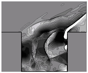
To study the role of waves, we conducted numerical simulations for the exchange between a recirculating flow on the side of a fast moving stream covering a range of mainstream Froude numbers varying from  $Fr_{o} = 0.2\text { to }4.5$. Figure 1 shows the top view of the simulation problem and vorticity patterns on a horizontal
  $x\text {--}y$ plane for several mainstream Froude numbers. Gravity is in the direction perpendicular to the plane. The depth and velocity of the mainstream are
  $H_o$ and
  $U_{o}$, respectively, and the dimension of the square basin is
  $L_b$. At low Froude numbers, the roll-up of the vortex sheet across the mixing layer to form eddies determines the exchange process. The mixing at higher Froude numbers is affected by the radiation of the waves from the mixing layer and the waves in the recirculating flow.

Figure 1. The exchange processes between the mainstream in a shallow open-channel flow and the recirculating flow in a square basin. The profiles of the vorticity,  $\zeta =\frac{\partial v}{\partial x} - \frac{\partial u}{\partial y} $, on the horizontal
  $x\text {--}y$ plane depict the exchanges for three different mainstream Froude numbers of (a)
  $Fr_{o} = 0.2$, (b)
  $Fr_{o} = 1.5$ and (c)
  $Fr_{o} = 3.0$. The red dashed lines in (b,c) mark the ‘Froude line’ with an oblique angle of
  $\theta =\sin ^{-1}(1/{ Fr}_{o})$.
We used a well-calibrated weighted essentially non-oscillatory (WENO) scheme to capture the shock waves while resolving turbulence in the mixing layer and the recirculating flow. Karimpour & Chu (Reference Karimpour and Chu2019) used this computational algorithm to examine the development of the free mixing layer between parallel streams. Their simulations were conducted for a range of convective Froude numbers,  $Fr_{ c} = (U_1-U_2)/(c_1+c_2)= 0.2\text { to }1.5$, where
  $U_1$ and
  $U_2$ are the velocities and
  $c_1$ and
  $c_2$ the celerity of gravity waves in the free streams on the sides of the free mixing layer. Their results have shown that the shock waves hinder the growth of the mixing layer. The gas-dynamic studies by Papamoschou & Roshko (Reference Papamoschou and Roshko1988), Samimy & Elliott (Reference Samimy and Elliott1990) and Pantano & Sarkar (Reference Pantano and Sarkar2002) for Mach numbers up to
  $Ma_{ c}$ = 1.1 have produced a similar reduction in the spreading rate of the free mixing layer between parallel air streams.
In the present simulation, tracer mass was introduced in the recirculating flow and monitored for its exchange with the mainstream during the simulation. The focus of the simulation was the determination of a retention time to compare with the laboratory measurements by Wang, Ghannadi & Chu (Reference Wang, Ghannadi and Chu2010) and Wang (Reference Wang2015). The experiments by Wang et al. (Reference Wang, Ghannadi and Chu2010) and Wang (Reference Wang2015) cover a range of Froude numbers varying from  $Fr_{o} = 0.2\text { to }3.5$. The paper has seven sections including this Introduction. Formulation of the shallow-water hydraulic model is given in § 2. Section 3 introduces a retention time to quantify the rate of the exchanges between the mainstream and the recirculating flow. The laboratory experiment and the correlation of a retention-time coefficient with the Froude number are given in § 4. A grid-refinement study is carried out in § 5 to determine the accuracy of the simulation. Section 6 shows the structure of the mixing layer and its interaction with the breaking shock waves within the recirculating flow. The final section contains the summary and conclusion.
2. Shallow-water hydraulic model
The numerical simulations for the exchanges were based on a shallow-water hydraulic model. The depth-averaged equations of the model are
 \begin{gather} \frac{\partial h}{\partial t}+\frac{\partial q_i}{\partial x_i} = 0, \end{gather}
 \begin{gather} \frac{\partial q_i}{\partial t}+ \frac{\partial (u_jq_i)}{\partial x_j}={-}gh \frac{\partial h}{\partial x_i}+ghS_{i}- \frac{c_f}{2} u_i\sqrt{u_ju_j} - \frac{1}{\rho} \left( \frac{\partial{h\tau_{ij}} }{\partial x_j} \right), \end{gather}
 \begin{gather} \frac{\partial ch}{\partial t}+\frac{\partial u_ich}{\partial x_i} = 0, \end{gather}
where  $h$ is the depth of the flow,
  $u_i$ are the velocity components in the
  $x_i$-directions,
  $q_i$ is the flow rate,
  $c$ is the tracer-mass concentration,
  $c_f$ is the bottom friction factor,
  $\rho$ is the density, and
  $g$ is gravity. The indices are
  $i=1,2$ and
  $j=1,2$. The components of the velocity and discharge are
  $u_i = (u_x, u_y)$ and
  $q_i= (q_x, q_y)$ for the two-dimensional flow on the
  $x\text {--}y$ plane. The channel slope
  $S_i=(S_o, 0)$ has only one component that is the longitudinal slope,
  $S_o$, in the
  $x$-direction. The repeated indices follow the tensor summation convention. We used the sub-grid-scale model by Vreman (Reference Vreman2004) to conduct the large-eddy simulation of the turbulent flow. In this model, the sub-grid-scale stresses,
  $\tau_{ij}$, and viscosity,
  $\nu_{sg}$, are
 \begin{gather} \tau_{ij} ={-} 2\nu_{sg}S_{ij} + \frac{1}{2} \delta_{ij} \tau_{kk} ={-} \nu_{sg}\left[\frac{\partial u_i}{\partial x_j}+\frac{\partial u_j}{\partial x_i}\right] + \frac{1}{2} \delta_{ij} \tau_{kk}, \end{gather}
 \begin{gather} \nu_{sg} = c\,\sqrt\frac{B_\beta}{\alpha_{ij}\,\alpha_{ij}}, \end{gather}
where
 \begin{equation} \alpha_{ij}= \frac{\partial {u_j}}{\partial{x_i}}, \quad \beta_{ij} = \Delta^2\,\alpha_{mi}\alpha_{mj} \quad \textrm{and} \quad B_{\beta}=\beta_{11}\,\beta_{22}-\beta_{12}^2. \end{equation}
The model constant  $c=2.5C_s^2$ and the value of the Smagorinsky constant is taken to be
  $C_s=0.2$. The sub-grid scale filter size,
  $\Delta$, is defined as
  $\Delta = \sqrt {\Delta x \Delta y}$. The coefficients in (2.6) were introduced by Vreman (Reference Vreman2004) to ensure that the sub-grid viscosity is small in laminar and shear flows and is not as dissipative as the well-known Smagorinsky eddy viscosity. Our computational algorithm calculates
  $\alpha _{ij}$ first from the velocity field. It subsequently, calculates
  $\beta _{ij}$, and ultimately the value of
  $B_{\beta }$.
We used the fifth-order WENO scheme by Shu (Reference Shu2009) for the spatial interpolations. The logarithmic law of the wall is assumed for the velocity and discharge profiles near the basin's boundaries. The time integration of the equations was conducted using a fourth-order Runge–Kutta method. The numerical method and the validation of the method for simulations of sub-critical and super-critical open-channel flow were given previously by Karimpour & Chu (Reference Karimpour and Chu2015).
The dimensions of the square basin are  $0.45\ \textrm {m} \times 0.45\ \textrm {m}$ and the basin is located 1.2 m downstream from the inlet of the main channel. The length and width of the open-channel main flow are 2.10 m and 3.00 m, respectively. The mesh sizes are
  ${\Delta } x$ =
  $\Delta y = 0.005\ \textrm {m}$. The depth of the main flow is
  $H_o= 0.042\ \textrm {m}$. The bottom friction coefficient has a value of
  ${c_f} = 0.008$. The longitudinal slope,
  $S_{o}$, of the open channel was selected to produce the desirable velocity
  $U_{o}$ and the Froude number,
  $Fr_{o}=U_o/\sqrt {gH_o}$, in the mainstream. The lateral slope of the channel is zero. Table 1 summarizes the parameters for 16 simulation cases and Froude numbers. The flow is uniform across the mainstream as it enters the computational domain. The outflow boundary condition is zero gradient. Figure 1 shows the vorticity profiles for three mainstream Froude numbers of (a)
  $Fr_{o} = 0.2$, (b)
  $Fr_{o} = 1.5$ and (c)
  $Fr_{o} = 3.0$. Waves were produced as the mainstream interacted with the recirculating flow in the square basin. For the cases of the super-critical mainstream as shown in (b,c), the mainstream was modified by oblique shock waves. The Froude lines with an angle of
  $\theta =\sin ^{-1}(1/{ Fr}_{o})$ in the figure mark the location of the oblique shock waves separating the undisturbed mainstream from the flow exchanging with the recirculating flow in the basin. The waves and turbulence produced by the exchange is complex but the overall exchange can be defined by a retention time as explained in the subsequent section.
Table 1. Summary of parameters for numerical cases. Grid-refinement studies are performed for cases 8-1, 8-2, 8-3 and 12-1, 12-2, 12-3 for  $Fr_{o}$ = 2.5 and 3.5, respectively.

3. Retention time
The retention time,  $\tau$, is a time scale introduced to characterize the exchange of the tracer mass in the recirculating flow with its external mainstream. It is defined by the fractional-rate equation as follows:
 \begin{equation} \frac{1}{\bar{c}}\frac{\textrm{d}\bar{c}}{\textrm{d}t}=\frac{1}{\tau}, \end{equation}
where  $\bar {c}$ is an average of tracer-mass concentration over an area in the recirculating flow. The solution to the fractional-rate equation is
 \begin{equation} \ln \left(\frac{\bar{c}}{c_o}\right) = \left( -{\frac{t}{\tau}} \right). \end{equation}
Booij (Reference Booij1989) used this retention time to characterize the exchange between a recirculating flow in a square basin and a sub-critical mainstream. The dimensionless parameter corresponding to retention time is the retention-time coefficient
 \begin{equation} C_{\tau}=\frac{\tau U_o}{L_b}. \end{equation}
 In the present simulation, tracer mass of uniform concentration,  $c_o$, was specified over the entire square basin at a time
  $t=t_1$, when the recirculating flow had reached the quasi-steady state. Figures 2(a), 2(b) and 2(c) show the subsequent instantaneous tracer-mass concentration distribution,
  $c(x, y, t)$, for the mainstream Froude numbers of
  $Fr_{o}= 0.2, 3.2$ and 3.8, respectively. The development of a mixing layer between the mainstream and the recirculating flow in the basin is responsible for the tracer-mass exchange. The entrainment of the fluids from two sides of the mixing layer led to the exchanges that caused the depletion of tracer mass in the basin. Figure 2(d) shows the basin-average dye concentration,
  $\bar {c}/c_o$, and its reduction with time,
  $(t-t_1)U_{o}/L_b$, on a semi-logarithmic scale for these three mainstream Froude numbers. Reduction in concentration with time perfectly matches the solution of the fractional-rate equation, (3.2). The retention-time coefficient,
  $C_{ \tau }$, was determined as the inverse slope of the straight lines, marked in the semi-logarithmic plots. This slope was maintained despite several orders of magnitude reduction in tracer-mass concentration,
  $\bar {c}/c_o$.

Figure 2. Sequence of images for the  ${c}/c_o$ distribution in the recirculating flow in the square basin for (a)
  $Fr_{o} = 0.2$, (b)
  $Fr_{o} = 3.2$ and (c)
  $Fr_{o} = 3.8$. (d) The average of the dye concentration over the square basin,
  $\bar {c}/c_o$, obtained from numerical simulation, and its reduction with the dimensionless time,
  $t^*=(t-t_1)U_{o}/L_b$, on a semi-logarithmic scale for
  $Fr_{o} = 0.2, 3.2$ and 3.8. Here,
  $t_1$ is the onset of quasi-steady state mixing and is when the tracer is introduced into the basin and
  $c_o$ is the initial tracer concentration at
  $t_1$.
Figure 2(d) demonstrates that the retention time is a unique parameter that can be identified for any Froude number. The values of the retention-time coefficient as defined by the inverse slopes of the lines in figure 2(d) are
 \begin{gather} C_{\tau}= 32, \quad \textrm{for} \ {Fr_ o}= 0.2, \end{gather}
 \begin{gather} C_{\tau}= 134, \quad \textrm{for} \ {Fr_ o}= 3.2, \end{gather}
 \begin{gather} C_{\tau}= 55,\quad \textrm{for} \ {Fr_ o}= 3.8. \end{gather}
This variation of the retention time with the Froude number is not monotonic. The retention-time coefficient increased from  $C_{\tau }=$ 32 to 134 from
  $Fr_{o}=$ 0.2 to 3.2, and then dropped sharply from
  $C_{\tau }=$ 134 to 55 as the Froude number varied only slightly from
  $Fr_{o}=$ 3.2 to 3.8.
The value of the retention-time coefficient,  $C_{ \tau } = 32$, for the sub-critical mainstream Froude number of
  $Fr_{o}=$ 0.2 was in agreement with the laboratory measurements by Booij (Reference Booij1989) and Altai & Chu (Reference Altai and Chu1997). The significant increase in the retention-time coefficient between
  $Fr_{o}=$ 0.2 and 3.2, by more than a factor of 4 from
  $C_{ \tau } =$ 32 to 134, is associated with the suppression of mixing-layer growth which, according to Karimpour & Chu (Reference Karimpour and Chu2019), is due to the radiation of waves from the mixing layer. This suppression of the mixing-layer growth is consistent with the analogous study in gas dynamics by Pantano & Sarkar (Reference Pantano and Sarkar2002). Figure 2(d) also shows a sharp drop in the retention-time coefficient from
  $Fr_{o}=$ 3.2 to 3.8. This drop cannot be explained by the suppression of growth in the mixing layer. The interaction of the mixing layer with the shock waves in the side basin affects the retention-time coefficient. The explanation of this sharp drop will be given later in § 6.
Figure 3 shows the dependence of the retention-time coefficient,  $C_{\tau }$, on the mainstream Froude number
  $Fr_{o}$ and the comparison of simulation results with the laboratory measurements. The retention-time coefficient increases with the Froude number from a value of
  $C_{\tau }= 32$ at
  $Fr_{o}= 0.2$ to a value of
  $C_{\tau }=$ 134 at
  $Fr_{o}= 3.2$. These simulation results over the range of
  $Fr_{o}=$ 0.2 to 3.0 are in support of the laboratory experiments by Wang et al. (Reference Wang, Ghannadi and Chu2010) and Wang (Reference Wang2015). But the most remarkable result shown in figure 3 is the ‘sharp drop’ in value of the retention-time coefficient from the value of
  $C_{\tau }= 134$ at
  $Fr_{o}= 3.2$ to a value of
  $C_{\tau }= 60$ at
  $Fr_{o}= 3.4$.

Figure 3. Non-monotonic variations of the retention-time coefficient,  $C_{\tau }=\tau U_{o}/L_b$, with the mainstream Froude number,
  $Fr_{o}$. The simulation results, denoted by the solid symbols, cover a range of Froude numbers varying from
  $Fr_{o}=$ 0.2 to 4.5. The laboratory measurements by Wang et al. (Reference Wang, Ghannadi and Chu2010) and Wang (Reference Wang2015), denoted by the open symbols, cover a smaller range of Froude numbers from
  $Fr_{o}=$ 0.2 to 3.5.
The irregularities in the increasing retention-time coefficient part in figure 3 cannot be attributed to computational inaccuracies. These are believed to be associated with the waves in the basin and their interactions with the mixing layer. The review paper by Rockwell & Naudascher (Reference Rockwell and Naudascher1978) has provided discussions on such interactions at low Mach numbers.
4. Comparison with laboratory experiments
Two sets of experimental data are presented in figure 3 that were obtained from two different experimental facilities. The experimental set-ups are illustrated in detail in Wang et al. (Reference Wang, Ghannadi and Chu2010) and Wang (Reference Wang2015). The retention-time coefficients obtained in the first series of experiments by Wang et al. (Reference Wang, Ghannadi and Chu2010), denoted by the open-diamond symbols in the figure, were generally higher than the coefficients obtained by the numerical simulation. The coefficients obtained in the later series of experiments by Wang (Reference Wang2015), denoted by the open-square symbols, however, were lower in value than the numerical results. The experiments by Wang et al. (Reference Wang, Ghannadi and Chu2010) were conducted a number of years earlier in a different facility from the experiments conducted later by Wang (Reference Wang2015).
The earlier experiments by Wang et al. (Reference Wang, Ghannadi and Chu2010) were conducted in a 142 cm wide channel. The dimensions of the basin on the side were  $15\ \textrm {cm}\times 15\ \textrm {cm}$ and the basin was located immediately after the entrance to the main channel. The retention time was determined in the earlier experiments based on the average of the tracer-mass concentration over a small central region,
  $\bar {c}_c$. Figure 4 shows the small central region in the basin that was used to determine the average concentration,
  $\bar {c}_c$. The retention-time coefficient was determined by curve fitting the data with (3.2). In these experiments, rhodamine red dye was introduced into the basin with an initial concentration
  $c_o$ and a dye flow rate
  $q_o$ for a period of time until the concentration in the basin had reached a quasi-steady state. The concentration of the red dye was determined using the video imaging method developed by Zhang & Chu (Reference Zhang and Chu2003) and Chu, Liu & Altai (Reference Chu, Liu and Altai2004). The presence of the red dye in the basin reduced the intensity of the green light. The percentage of the green-light intensity reduction was used to determine the dye concentration. The data denoted by the open symbols in the figure were the dimensionless concentration,
  $\bar {c}_c U_{o} L_b H/c_oq_o$, for an experiment with a mainstream Froude number of
  $Fr_{o}= 3.5$. The dashed line is (3.2) for
  $C_{\tau }=$ 145 that best fit the experimental data.

Figure 4. The determination of the retention-time coefficient in the laboratory experiment by Wang et al. (Reference Wang, Ghannadi and Chu2010) for  $Fr_{o}= 3.5$. The average concentration,
  $\bar {c}_c$, was obtained in the central region of the basin marked by the square symbols. The dashed line is the (3.2) for
  $C_{\tau }$ = 145 that fits the experimental data.
The later experiments by Wang (Reference Wang2015) were conducted in a smaller channel. The width of the small channel was only 35.5 cm. The basin dimension for the smaller facility was  $24\ \textrm {cm} \times 24\ \textrm {cm}$. The retention time was determined in the later experiment based on the average of the tracer-mass concentration over the entire basin,
  $\bar {c}$. The super-critical flow was produced using a sluice gate in this facility. In the super-critical range, large surface waves were produced by the edges of the sluice gate. The disturbances caused by the surface waves in the narrow main channel produced great penetration to the mixing layer. This might have caused the retention-time coefficient obtained in the experiments by Wang (Reference Wang2015) to be slightly lower than the results of the numerical simulation.
Furthermore, Wang et al. (Reference Wang, Ghannadi and Chu2010) obtained the retention-time coefficient using the concentration averaged over a small area in the core region of the recirculating flow. The entrapment of the tracer dye in the core region is more persistent than in the outer region. This explains further why the retention-time coefficients,  $C_{\tau }$, obtained by Wang et al. (Reference Wang, Ghannadi and Chu2010) were generally higher than those in the numerical simulation. Despite the difference in the experimental set-ups, both experiments produced retention-time coefficients that follow a similar trend of dependence on the mainstream Froude number,
  $Fr_{o}$, as the trend of dependence in the simulation, up to a Froude number of approximately
  $Fr_{o} \simeq$ 3.0.
In both experiments, the dye concentration was estimated based on a calibration curve. Red dye of known concentration was placed in a calibration box. The calibration curve is a relationship between the reduction of green-light intensity in the video image and the known dye concentrations. This video imaging method is affected by the presence of surface waves. For super-critical flow of high Froude number, the amplitude of the wave was comparable to the water depth and the accuracy of the video imaging is compromised. To compensate for the wave's effect, an artificial disturbance was introduced to the water in the calibration box. Such an artificial disturbance in the box cannot perfectly replicate the surface waves in the square basin at large Froude numbers. We believe that this has partly contributed to discrepancies between numerical simulations and laboratory measurements.
We have experienced difficulties of measuring the dye concentration at high Froude numbers. The free-surface waves that obscured the incident and reflected light beams were very large in amplitude for Froude numbers greater than 3.5. For this reason, Wang (Reference Wang2015) and Wang et al. (Reference Wang, Ghannadi and Chu2010) did not report any experimental data beyond  $Fr_{o}= 3.5$.
5. Grid-refinement study
To corroborate the unexpected result, we conducted a grid-refinement study for a Froude number  $Fr_{o}= 2.5$, before the sharp drop in value of the retention-time coefficient, and at Froude number
  $Fr_{o}= 3.5$, immediately after the drop. The refinement ratio, the corresponding retention coefficient, the order of convergence (P) and the fractional error (FE) are presented in table 2. The convergent values, as defined by Karimpour & Chu (Reference Karimpour and Chu2015), were for
  $\tau U_{o}/L_b = 56.85$ and 118.5 at
  $Fr_{o}= 3.5$ and 2.5, respectively. The respective fractional error and order of convergence were
  $\textrm {FE}(\%) = 0.22$ and 0.11, and
  $\textrm {P} = 2.5$ and 2.9. The grid-refinement study not only established the accuracy of the numerical simulation, it also ascertained the existence of the sharp drop in value of the retention-time coefficient from
  $C_{\tau } =\tau U_{o}/L_b=$ 118 to 57 across the changes in Froude number from
  $Fr_{o}$ = 2.5 to 3.5. The simulation results presented in figure 3 were obtained using
  $N= 1.0/\Delta x = 200$ nodal points.
Table 2. The mesh-refinement study for the accuracy and order of convergence conducted for the two mainstream Froude numbers of  $Fr_{o} = 2.5$ (cases 8-1, 8-2 and 8-3) and 3.5 (cases 12-1, 12-2 and 12-3) before and after the ‘sharp drop’ in the value of
  $\tau U_{o}/L_b$.

6. Discussion
We have shown how the retention time is a uniquely defined parameter that characterizes the exchange between the recirculating flow and the mainstream. The retention-time coefficient increased from a value of  $C_{\tau } \simeq 32$ at
  $Fr_{o}= 0.2$ to a value of
  $C_{ \tau } \simeq 134$ at
  $Fr_{o}= 3.2$. This then was followed by a ‘sharp drop’ to the value of
  $C_{ \tau } \simeq 61$ at
  $Fr_{o}= 3.4$. This striking variation of the retention-time coefficient with the mainstream Froude number shown in figure 3 is associated with structural changes in the mixing layer and the recirculating flow as explained in the following sub-sections.
6.1. The mixing layer between the mainstream and the recirculating flow
The vorticity and the tracer-mass concentration profiles in figures 1 and 2 delineate the structural dependence of the flow on the mainstream Froude number. The sub-critical exchanges at  $Fr_{o}=$ 0.2, as shown in figures 1(a) and 2(a), were associated with the coherent eddies in the mixing layer. The eddies coalesced to form bigger eddies in the mixing layer as the fluid was drawn into the mixing layer through a process known as entrainment, from the mainstream on one side and from the recirculating flow in the basin on the other side.
Studies of free mixing layers between parallel streams by Karimpour & Chu (Reference Karimpour and Chu2019) and Pantano & Sarkar (Reference Pantano and Sarkar2002) have found that the spreading rate is reduced by the radiation of waves from the mixing layers. Similar effect on the spreading rate may occur in the mixing layer between the mainstream and the recirculating flow and this may explain the consistent increase in the retention-time coefficient with the mainstream Froude number from  $Fr_{o}=$ 0.2 to 3.2.
The lateral spreading of the mixing layer is affected by the wave radiation from the mixing layer. With radiation of the wave energy, less energy is available for the production of turbulence in the mixing layer. The mixing layers of higher Froude numbers were relatively less energetic and, therefore, made less contribution to the exchange processes. The suppression of turbulence in the mixing layer can explain the increase in the retention-time coefficient with the mainstream Froude number. This, however, cannot explain the ‘sharp drop’ in value of the retention-time coefficient from  $Fr_{o}= 3.2$ to
  $Fr_{o}= 3.4$.
6.2. The occurrence of shock waves within the recirculating flow
The contours of the relative depth,  $h/H_o$, in figures 5(a), 5(b), and 5(c) delineate further the interaction between the eddies and waves for the cases with the mainstream Froude numbers
  $Fr_{o}=$ 0.2, 1.5 and 4.5, respectively. For the sub-critical flow with
  $Fr_{o}= 0.2$, the depth fluctuations in the range of
  $h/H_o\simeq 1 \pm 0.07$ were quite small. The depth fluctuations increased with the Froude number to
  $h/H_o\simeq 1 \pm 0.24$ for
  $Fr_{o}= 2.0$ and then to
  $h/H_o\simeq 1 \pm 0.48$ for
  $Fr_{o}= 4.5$. For the mainstream with the large Froude number of
  $Fr_{o}=$ 4.5, shock waves of significant amplitude were observed to occur within the recirculating flow in the basin. The wave height of the shock waves,
  $(h_{ max}-h_{ min})/H_o \simeq 0.96$, in this case was comparable to the mean depth.

Figure 5. The eddies and waves as defined by the depth  $h/H$ for the mainstreams with (a)
  $Fr_{o} = 0.2$, (b)
  $Fr_{o} = 2.0$ and (c)
  $Fr_{o} = 4.5$. The red dashed lines in (b,c) are the ‘Froude lines’ separating the undisturbed mainstream from exchange flow with the recirculating flow in the basin.
The ‘sharp drop’ in retention-time coefficient was associated with a major structural change in the recirculating flow. We examine this structural change in figures 6(a) and 6(b) using the local Froude number  $Fr = \sqrt {u^2+v^2}/\sqrt {gh}$ as the indicator. The distinction between flow shown in figure 6(a) with the mainstream Froude number of
  $Fr_{o}= 2.0$ and the flow shown in figure 6(b) of
  $Fr_{o}= 4.5$ is the formation of shock waves inside the basin. The red colour in the contours defines the area where the local Froude number is
  $Fr>1$. The blue colour, on the other hand, defines the area where the local Froude number is
  $Fr<1$. The change in blue to red defines the front of the shock waves in this figure.

Figure 6. The wave dynamics in the recirculating flow as delineated by the local Froude number  $Fr = \sqrt {u^2+v^2}/\sqrt {gh}$ shown at 10 s intervals, (a) for
  $Fr_{o}$ = 2.0 before the sharp drop and (b) for
  $Fr_{o} = 4.5$ after the sharp drop. The corresponding velocity profile for
  $u/U_{o}$ across the flow at the mid-section (
 $x = L_b/2$) is in (c,d).
The recirculating flow in case (a) with a  $Fr_{o}= 2.0$, had a nearly stagnant core. The local Froude number in the core defined by the blue colour is nearly zero. The tracer mass entrapped in the stagnant core was not accessible for exchange across the mixing layer. The circulation mainly around the edge of the basin was relatively steady with fewer waves in the circulation.
The velocity of the recirculating flow was much higher in case (b) with  $Fr_{o}= 4.5$. The local Froude number is rapidly changing from the sub-critical (blue) to super-critical (red). Shock waves of large amplitude were observed contributing to mixing throughout the entire basin. The large-amplitude shock waves in the basin and their interaction with the mixing layer promoted the exchanges leading to the sharp drop in the value of the retention-time coefficient at
  $Fr_{o}= 3.4$ (between the
  $Fr_{o}= 2.0$ and 4.5).
The magnitude of the recirculating velocity in the basin was approximately equal to one third of the mainstream velocity,  $U_o$, as shown in figures 6(c) and 6(d) for mainstream Froude numbers of
  $Fr_{o}$ = 2.0 and 4.5. Therefore, the local Froude number in the recirculating area would begin to exceed the critical value of unity when the mainstream Froude number exceeds
  $Fr_{o} \simeq 3.0$. The interaction of these shock waves in the basin with the mixing layer is believed to be the reason for the sudden increase in the exchange and the sharp drop in the value of retention-time coefficient at the mainstream Froude number of approximately
  $Fr_{o}= 3.4$.
7. Summary and conclusion
We conducted numerical simulations of the recirculating flow in a square basin using a shallow-water hydraulic model for a range of mainstream Froude numbers varying from  $Fr_{o}=$ 0.2 to 4.5. A retention-time coefficient was introduced to characterize the exchange of mass across the mixing layer. Two distinct ranges of dependence on Froude number have been observed: (i) the value of the retention-time coefficient increased with the Froude number over the range of
  $Fr_{o}=$ 0.2 to 3.2, and (ii) a sharp drop in the value of the coefficient occurred at a Froude number of
  $Fr_{o} \simeq 3.4$. The increase in values of the retention-time coefficient over the range of
  $Fr_{o}=$ 0.2 to 3.2 is due to the suppression of turbulence production in the mixing layer. The sharp drop, on the other hand, is associated with the formation of shock waves within the recirculating flow in the basin and the interaction of these shock waves with the mixing layer. The laboratory observation is consistent with the numerical simulations in the range of Froude number from
  $Fr_{o}$= 0.2 to 3.0.
This is the first study highlighting the role of shock waves within a recirculating flow on the exchange process with the mainstream. Geometrical variations of the basin produced by the length-to-width ratio, the change in depth within the basin and the existence of adjacent basins, have effects on the exchange processes and the sudden drop in the retention-time coefficient. The role of these variations has been studied in subcritical flows by Uijttewaal et al. (Reference Uijttewaal, Lehmann and van Mazijk2001). Further studies are required to investigate their role in the exchange process for supercritical flows of high Froude numbers.
The shallow-water hydraulic model had reproduced the flow at low mainstream Froude number when the exchange was governed by the production of coherent eddies and roll-up of the vortex sheet in the mixing layer. The model was also capable of producing the waves when the exchange process was affected by the shock waves in the basin. The success of the numerical simulations for the high-speed shear flow is attributable to the reliable shock capture schemes developed by Karimpour & Chu (Reference Karimpour and Chu2015) for the numerical simulations. Karimpour & Chu (Reference Karimpour and Chu2014) used this shallow-water hydraulic model to find the lateral discharge from a side weir in an open-channel flow. Their results produced discharge coefficients in perfect agreement with those of laboratory experiments. Karimpour & Chu (Reference Karimpour and Chu2016, Reference Karimpour and Chu2019) studied the role of waves on the development of the free mixing layer using the same computational algorithm. Their results for open-channel flow were validated by the observations made in the analogous gas-dynamic problem. The present simulation is an additional piece of evidence supporting the general use of the model for simulation of shallow shear flows over a wide range of Froude numbers.
Declaration of interests
The authors report no conflict of interest.


