2. Governing equations

We consider only the flow beneath the evaporating surface and as such the working fluid is liquid water, which is treated as Newtonian. We investigate flows without invoking the Oberbeck–Boussinesq approximation and therefore take into account variations of the density and transport properties with temperature. For this reason, the system of governing equations is the low Mach number approximation of the compressible Navier–Stokes–Fourier equations (Majda & Sethian Reference Majda and Sethian1985; Lessani & Papalexandris Reference Lessani and Papalexandris2006)

(2.1)\begin{gather} \frac{\partial\rho}{\partial t} + \boldsymbol{\nabla} \boldsymbol{\cdot} \left(\rho \boldsymbol{u} \right) =0, \end{gather}

(2.2)\begin{gather}\frac{\partial \!\left( \rho \boldsymbol{u} \right)}{\partial t} + \boldsymbol{\nabla} \boldsymbol{\cdot} \left(\rho {\boldsymbol{uu}} \right) =\boldsymbol{\nabla} \boldsymbol{\cdot} {\boldsymbol{\tau}} - \boldsymbol{\nabla} p + \rho \boldsymbol{g}, \end{gather}

(2.3)\begin{gather}\frac{\partial \!\left( \rho c_p T \right)}{\partial t} + \boldsymbol{\nabla} \boldsymbol{\cdot} \left( \rho c_p \boldsymbol{u} T \right) = \boldsymbol{\nabla} \boldsymbol{\cdot} \left( \lambda \boldsymbol{\nabla} T \right) + \frac{\textrm{d}p_0 \left(t \right)}{\textrm{d} t}, \end{gather}

where ρ stands for the fluid density and $\boldsymbol {u}=(u,v,w)$ for the fluid velocity vector. In (2.2), $p$ stands for the sum of the second-order term of the low Mach number expansion of the pressure and the bulk viscous pressure (Georgiou & Papalexandris Reference Georgiou and Papalexandris2018; Papalexandris Reference Papalexandris2019). Also ${\boldsymbol {\tau }}$, stands for the deviatoric part of the viscous stress tensor, defined as ${\boldsymbol {\tau }} = \mu ( \boldsymbol {\nabla } \boldsymbol {u} + ( \boldsymbol {\nabla } \boldsymbol {u} )^\textrm {T} -\frac {2}{3} ( \boldsymbol {\nabla } \boldsymbol {\cdot } \boldsymbol {u} ) {\boldsymbol {I}} )$, where ${\boldsymbol {I}}$ is the identity matrix and $\mu$ the dynamic viscosity.

In (2.3), $c_p$ is the specific heat, $\lambda$ the thermal conductivity and $p_0(t)$ the first-order component of the asymptotic expansion of pressure at the zero Mach limit, interpreted as the thermodynamic pressure. According to the low Mach number expansion, it is spatially uniform and a function of time only. For open domains, $p_0$ is equal to the ambient pressure whereas for closed domains, $p_0$ varies with time and can be computed from the equation of state of the working medium. In this study the domain is open. For this reason, $p_0$ is constant and set to the ambient pressure of one atmosphere. We note that the mass loss leaving the system due to evaporation is not modelled and the surface level is constant throughout. For the highest evaporation case the mass loss through the free surface would be equivalent to 3 %. This is considered to have a minor effect on the free-surface level over the simulation times considered.

In order to close the system of governing equations, an isobaric ‘equation of state’ for the water density is required. More specifically, a $\rho -T$ relation is introduced. This relation is a fourth-order polynomial fit (2.4) of the tabulated data in (Lemmon et al. Reference Lemmon, Huber and McLinden2010) for water density at one atmosphere and over the temperature range of interest. The other fluid thermodynamic properties, $\lambda$ and $\mu$ are also calculated from a quartic polynomial fit of the form (2.4) with data originating from the same reference. For a generic quantity $\phi$, this fit reads

(2.4)\begin{equation} \phi =c_4 T^4 + c_3 T^3 + c_2 T^2 + c_1 T + c_0 . \end{equation}

An example set of coefficients for the fits of $\rho /p_{0}$, $\lambda$ and $\mu$ are provided in table 8 of the Appendix.

For the case with the largest ${\rm \Delta} T$, the dynamic viscosity and the thermal conductivity vary respectively by 24 % and 2 % over the temperature range of interest. In other words, even though the density variations are small, the induced variations in the transport properties of water are non-negligible. On the other hand, $c_p$ varies by a maximum of only 0.4 % over the maximum temperature range investigated. It is thus taken as a constant, case-dependent, value in all simulations; see table 8. We note that with the aforementioned variations in fluid properties, $Pr$ varies by 26 % across the domain for the highest evaporation case.

For the numerical solution of (2.1)–(2.3) we employ a second-order accurate time-integration scheme for convective and diffusive terms, taking into account the current and the two previous time steps. Regarding the spatial discretization, the governing equations are discretized using second-order central difference schemes on a collocated grid system. A flux interpolation technique is used in the spirit of Rhie & Chow (Reference Rhie and Chow1983), to avoid pressure odd–even decoupling (Weller et al. Reference Weller, Tabor, Jasak and Fureby1998; Lessani & Papalexandris Reference Lessani and Papalexandris2006, Reference Lessani and Papalexandris2008).

For the pressure–velocity coupling a Pressure-Implicit with Splitting of Operators (PISO) projection method is used, similar to the methods proposed by Issa (Reference Issa1985) and Oliviera & Issa (Reference Oliviera and Issa2001) for incompressible flows. The divergence of the momentum equation is taken and the continuity equation is used as a constraint to formulate the variable-coefficient Poisson equation to be solved for $p$. In this low Mach number PISO algorithm, the temporal derivative of the density, $\partial \rho /\partial t$, emerges on the left-hand side of the Poisson equation which would be zero for the incompressible case.

3. Estimation of evaporation rates

For specified thermal boundary conditions at the walls of the pool and for given ambient conditions, the evaporation rate depends on the gas-side transport phenomena. In the present work, however, the focus is not on such phenomena but on the thermal mixing water side. For this reason, we only solve for the flow field below the free surface, referred to interchangeably herein as the interface. This in turn requires the mean temperature at the interface to be specified, from which the evaporation rates and temperature gradients at the interface can then be estimated. Also for a given mean interface temperature, the bottom wall temperature is not known in advance and must be estimated a priori on a case-by-case basis. As first approximations we take estimations from high surface temperature evaporation experiments, where data are provided for temperature drops across water domains during evaporation. These are subsequently refined in preliminary simulations until the correct temperature drop is found.

In this section we obtain realistic approximations of the heat losses at the upper boundary, as well as the corresponding lower wall temperatures. This will enable the assignment of thermal boundary conditions in the following section. To estimate these quantities we start with an energy balance across the interface which provides the following relation:

(3.1)\begin{equation} \dot{q}^{\prime\prime}_{add} = \dot{q}^{\prime\prime}_{conv} +\dot{q}^{\prime\prime}_{evap}. \end{equation}

Here, the right-hand side terms, $\dot {q}^{\prime \prime }_{conv}$ and $\dot {q}^{\prime \prime }_{evap}$, represent respectively the convective and latent heat losses per unit surface area to the ambient gas-side environment. The left-hand side term, $\dot {q}^{\prime \prime }_{add}$, represents the heat added to the interface from the water side. By expanding this latter quantity and $\dot {q}^{\prime \prime }_{evap}$, we arrive at the following:

(3.2)\begin{equation} \left.\frac{\overline{\partial T}}{\partial y}\right|_{w} = \frac{1}{\lambda_{w}}\left(\dot{q}^{\prime\prime}_{conv} + \dot{m}^{\prime\prime} h_{lv} \right), \end{equation}

where $\dot {m}^{\prime \prime }$ is the evaporative mass flux, $h_{lv}$ is the interface-temperature-dependent latent heat of evaporation and $\lambda _{w} \overline {\partial T/ \partial y} \vert _{w}$ is the mean heat flux at the water side of the interface, with $\lambda _{w}$ as the thermal conductivity of water at the mean interface temperature, $T_{int}$. The task is then to find approximations for the right-hand side terms in (3.2) which will form the basis of our non-zero Neumann boundary condition.

As a first step in calculating $\dot {q}^{\prime \prime }_{evap}$ we fix the gas-side conditions at a distance far from the interface. Estimates are taken from the experimental work of Martin & Migot (Reference Martin and Migot2019) investigating high temperature evaporation, with values provided in table 9 of the Appendix. In this table, $T_{\infty }$ is the temperature far from the interface and $p_{0}$ is the thermodynamic pressure. The water vapour partial pressure, $p_{v,\infty }$, is calculated from a Wagner equation (Poling, Prausnitz & O’Connell Reference Poling, Prausnitz and O'Connell2001), before taking into account the relative humidity, RH, also provided in table 9. The water vapour mass fraction far from the interface, $Y_{v,\infty }$, can then be found from the following relation:

(3.3)\begin{equation} Y_{v} = \frac{p_{v} M_{w}}{p_{v} M_{w} + (p_0 - p_{v}) M_{a}} , \end{equation}

where $M_{w}$ and $M_{a}$ are respectively the molar masses of water and air. Assuming a binary mixture of water vapour and air, the mass fraction of air at the same location is found from $1-Y_{v,\infty }$. The gaseous mixture density far from the interface, $\rho _{\infty }$, is calculated from the mass fractions and the ideal-gas equation of state and is given in table 9 of the Appendix. Equivalently, we set the conditions at the interface representative of different evaporation fluxes. First, $T_{int}$ is selected and a corresponding saturation pressure, $p_{v,int}$, is found. The vapour mass fraction, $Y_{v,int}$, and mixture density, $\rho _{int}$, are then calculated as above with values provided in table 10 of the Appendix.

We assume that, on the gas side, the transition from the interface conditions to those far away takes place within a layer of finite thickness, referred to herein as a film. Finding the mean of the interface values and those at a distance far away allows for an estimation of the film properties. We require the quantities of $\rho _{f}$, ${c_p}_{f}$, $\mu _{f}$ and $\lambda _{f}$, representing respectively the film density, specific heat, dynamic viscosity and thermal conductivity. Of these, both $\rho _{f}$ and ${c_p}_{f}$ are mass averaged using the film mass fraction, $Y_{v, f}$, whereas the quantities of $\mu _{f}$ and $\lambda _{f}$ are found from the kinetic theory of gases; see Wilke (Reference Wilke1950) and Mason & Saxena (Reference Mason and Saxena1958), respectively. The film diffusion coefficients for momentum, $\nu _{f}$, and energy, $\kappa _{f}$, respectively the kinematic viscosity and the thermal diffusivity are then found from a combination of the aforementioned properties. Finally, the film mass diffusivity for the binary mixture of air and vapour, $D_{f}$, is found from the following relation (Marrero & Mason Reference Marrero and Mason1972):

(3.4)\begin{equation} D_{f} = 1.87 \times 10^{-10}\, \frac{T^{2.072}_{f}}{p_0}\quad \left(\frac{\textrm{m}^2}{\textrm{s}}\right) , \end{equation}

where the thermodynamic pressure, $p_0$, is equal to 1 atm. The film diffusion coefficients are used to find the film Prandtl ($Pr_{f}$), Schmidt ($Sc_{f}$) and Lewis ($Le_{f}$) numbers, all of which are provided in table 1. For all cases examined herein, it was assumed that $Le = 1$, implying that the concentration and thermal boundary layer heights above the interface are equal. This allows us to find a gas-side concentration Rayleigh number using properties based on the local water vapour mass fraction and temperature.

Table 1. Gas-side dimensionless parameters. In this table $Pr_{f} = \nu _{f}/\alpha _{f}$, $Sc_{f} = \nu _{f}/D_{f}$ and $Le = Sc_{f}/Pr_{f}$. The non-dimensional groups $Ra_{c}$, $Sh$, $Ra_{t}$ and $Nu_{t}$ are defined in the text.

Pertinent experimental studies of free-surface evaporation include Boelter et al. (Reference Boelter, Gordon and Griffin1946) and Bower & Saylor (Reference Bower and Saylor2009). Both measured evaporation rates into a quiescent air environment; however, Bower & Saylor (Reference Bower and Saylor2009) used an improved set-up, allowing for more realistic air-side natural convection conditions. Both papers provide Sherwood number ($Sh$) correlations based on a relationship with the Schmidt number ($Sc$) and the concentration Rayleigh number, $Ra_{c}$, defined as follows:

(3.5)\begin{equation} Ra_{c} = \frac{|{\boldsymbol{g}}| \left(\rho_{\infty} - \rho_{int} \right) W^3}{D_{f} \mu_{f}} . \end{equation}

Bower & Saylor (Reference Bower and Saylor2009) then proposed the following correlation, used here to find an estimation of the concentration boundary layer height, $\delta _{c}$,

(3.6)\begin{equation} Sh = 0.23Sc^{0.333}{Ra_{c}}^{0.321} \approx \frac{W}{\delta_{c}}. \end{equation}

The fact that $Sh$ is inversely proportional to the height of the concentration boundary layer is again an analogy with heat transfer that holds in cases with $Le=1$. The mass flux can then be estimated with the following relation (Lienhard & Lienhard Reference Lienhard IV and Lienhard V2019):

(3.7)\begin{equation} \dot{m}^{\prime\prime} = \frac{\rho_{f} D_{f}}{\delta_{c}} \log \left( 1 + B_{m}\right), \end{equation}

with the mass transfer driving force, $B_{m}$, defined as

(3.8)\begin{equation} B_{m} = \left(\frac{Y_{v,\infty} - Y_{v,int}}{Y_{v,int} - 1}\right) . \end{equation}

Substituting (3.6) into (3.7) gives the following relation for the mass flux:

(3.9)\begin{equation} \dot{m}^{\prime\prime} = Sh \frac{ \rho_{f} D_{f}}{W} \log \left( 1 + B_{m}\right) . \end{equation}

The latent heat flux is then found from $\dot {q}^{\prime \prime }_{evap} = \dot {m}^{\prime \prime } h_{lv}$ and the final heat and mass fluxes are provided in table 2.

Table 2. Fluxes at the interface. In this table $\dot {m}^{\prime \prime }$ is the mass flux, $\dot {q}^{\prime \prime }_{evap}$ is the evaporative heat flux and $\dot {q}^{\prime \prime }_{conv}$ is the convective heat flux. The prescribed temperature gradient, $\overline {\partial T/ \partial y} \vert _{w}$, is the dimensional form of the non-zero Neumann upper thermal boundary condition. The values are rounded to the nearest thousand to highlight their approximate nature.

Next, the convective heat loss is estimated by assuming that it is proportional to the difference between the temperature of the interface, $T_{int}$, and the ambient gas-side temperature, $T_{\infty }$, with the heat transfer coefficient, $h$, as the proportionality coefficient. Overall we have the following:

(3.10)\begin{equation} \dot{q}^{\prime\prime}_{conv} = h\!\left(T_{int} - T_{\infty}\right) , \end{equation}

where $h$ is estimated from the following correlation for a horizontal flat surface that is warmer than the ambient air above (Lloyd & Moran Reference Lloyd and Moran1974),

(3.11)\begin{equation} \frac{h W}{ \lambda_{f}} = Nu_{t} = 0.54 {Ra_{t}}^{0.25}. \end{equation}

In the above relation, $Ra_{t}$ is the gas-side thermal Rayleigh number,

(3.12)\begin{equation} Ra_{t} = \frac{|{\boldsymbol{g}}| \beta_{\infty} \left(T_{int} - T_{\infty}\right) W^3 }{ \kappa_{f} \nu_{f}} , \end{equation}

and $W$ is the characteristic length scale, the width of the domain. We provide values for $Ra_{t}$ and $Nu_{t}$ in table 1 and $\dot {q}^{\prime \prime }_{conv}$ in table 2.

With the upper temperature gradient known, it remains to find an estimate for the corresponding case-dependent lower wall temperatures, $T_{low}$. Martin & Migot (Reference Martin and Migot2019) carried out evaporation experiments of water at high surface temperatures and measured the temperature drop between the water bulk and the interface, ${\rm \Delta} T_{u} = T_{bulk}-T_{int}$. They reported that the temperature drop from the interface to the bulk increases in a nonlinear manner with increasing evaporation rate. They also observed that the temperature drop between the heated lower wall and the bulk, ${\rm \Delta} T_{l} = T_{low} - T_{bulk}$, was approximately equal to that between the bulk and the interface. That is, ${\rm \Delta} T_{l} \approx {\rm \Delta} T_{u}$. Therefore, in our configuration, the total temperature difference across the pool is first approximated as follows:

(3.13)\begin{equation} {\rm \Delta} T = T_{low}-T_{int} = 2{\rm \Delta} T_{u}, \end{equation}

with ${\rm \Delta} T_{u}$ estimated from the experiments of Martin & Migot (Reference Martin and Migot2019).

This first approximation is updated in preliminary simulations until the correct time- and area-averaged $T_{int}$ is found. As ${\rm \Delta} T_{u}$ was reported to increase with evaporation rates, the lower wall temperature, $T_{low}$ is case dependent. A physical explanation for this is seen in (3.1), where a higher evaporation flux is only possible with more heat added to the interface from below. In the current configuration, this energy addition must be via an increase in $T_{low}$. The lower wall temperatures are provided in table 3, alongside the predicted time- and area-averaged $T_{int}$.

Table 3. Thermal boundary conditions: in this table $T_{int}$ is the predicted interface value, $T_{low}$ is the fixed lower wall temperature and $T_{ref}$ is the mean pool temperature. The normalized temperature is defined as $\hat {\theta }=(T-T_{ref})/{\rm \Delta} T$, so that the upper and lower boundary values correspond to $\hat {\theta }_{int} = -0.5$ and $\hat {\theta }_{low} = 0.5$, respectively, for all cases.

It is worth adding here an observation of Boelter et al. (Reference Boelter, Gordon and Griffin1946), that evaporation measurements were invalidated above an upper physical limit. In their experiments boiling at the lower wall began at bulk water temperatures in excess of 361.15 K. In table 3, we see that the $T_{low}$ of case 5 exceeds this limit; the results for this case are therefore caveated but are included to explore the parameter space more completely. At the other end of the scale, the smallest $Ra$ investigated herein corresponds to an interface temperature of 40 K. At lower temperatures, the associated evaporation rate produces too small a ${\rm \Delta} T$ to drive turbulent convection below.

Finally, we define the normalized temperature as follows:

(3.14)\begin{equation} \hat{\theta} = (T-T_{ref})/{\rm \Delta} T, \end{equation}

with $T_{ref}$ as the mean of the lower wall and interface temperatures. If the estimations of the evaporative heat losses and corresponding lower wall temperatures are correct, we have $\hat {\theta }_{int} = -0.5$ and $\hat {\theta }_{low} = 0.5$, at the statistically stationary solution.

4. Numerical set-up

The computational domain is a cube of unity aspect ratio. As mentioned in the introduction, deviations away from the classical turbulent RBC set-up in the current configuration are in both the hydrodynamic and thermal boundary conditions prescribed at the upper boundary. Before expanding on this, we introduce dimensionless variables denoted by a hat ($\widehat {..}$) and provide reference values used for non-dimensionalization purposes in table 4. The reference length is the height of the cube, $H$, and is constant for all cases. With the reference velocity as the free-fall velocity, $U_{ff} = \sqrt {|{\boldsymbol {g}}| H \beta _{ref} {\rm \Delta} T}$, we find a reference free-fall time from $t_{ff} = H/U_{ff}$. Finally, the reference temperature is the mean in the pool, $T_{ref}$, with all reference properties then relative to $T_{ref}$.

Table 4. Reference values for non-dimensionalization purposes. The reference height, $H$, is 0.045 m for all cases.

The lower wall is located at $\hat {y}=0$, the upper boundary at $\hat {y}=1$ and, likewise, the sidewalls at $\hat {x}=0$ ($\hat {z}=0$) and $\hat {x}=1$ ($\hat {z}=1$). No-slip velocity boundary conditions are enforced at the side and lower walls. The free-slip condition is prescribed at the upper boundary, i.e. $\partial \hat {u}/\partial \hat {y} = \partial \hat {w}/\partial {\hat {y}} = 0$ and $\hat {v}=0$ at $\hat {y}=1$. This can be considered as a first-order approximation of a free surface. For the thermal boundary conditions outlined in the previous section we have adiabatic sidewalls with $\partial \hat {\theta }/\partial {\hat {x}}$ prescribed. At $\hat {y}=0$ we set $\hat {\theta }=0.5$ as a Dirichlet boundary condition, whereas at $\hat {y}=1$ we prescribe the non-zero Neumann conditions provided in table 2. The non-dimensional form of the prescribed temperature gradients are found by dividing by the case-specific ${\rm \Delta} T/H$, which gives $\partial \hat {\theta }/\partial {\hat {y}} = 21.4$, $25.7$, $38.6$, $45.0$ and $50.4$ for cases 1–5, respectively.

As a result of the aforementioned boundary conditions, five hydrodynamic boundary layers exist, one at each of the vertical sidewalls and one at the lower wall. On the other hand, there are only two thermal boundary layers, at the cooled upper boundary and heated lower wall. Finally, and with regard to the initial conditions, a linear temperature profile from $T_{low}$ to $T_{int}$ is employed across the vertical direction, whereas for the velocity a quiescent field is enforced to which small random perturbations are applied.

The Rayleigh number is then calculated as follows:

(4.1)\begin{equation} Ra= \frac{g \beta_{ref} (T_{low} - T_{int}) H^3 }{\nu_{ref} \kappa_{ref} } , \end{equation}

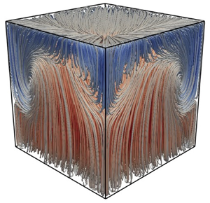
with the ${\rm \Delta} T$ now specific to our boundaries. We provide values for $Ra$ in table 3 and herein refer to cases 1–5 via their corresponding $Ra$. An instantaneous view of typical temperature isosurfaces are presented in figure 2 for the cases of $Ra=1.5\times 10^7$ and $Ra=9 \times 10^7$; smaller flow structures appear as evaporation is increased.

Figure 2. Instantaneous isosurfaces of the temperature field: (a) a low evaporation case corresponding to $Ra=1.5\times 10^7$ and (b) a high evaporation case corresponding to $Ra=9 \times 10^7$.

5. Resolution requirements

The accuracy of a DNS is ensured only when the smallest length scales of the flow are everywhere resolved. The first criterion is therefore to ensure adequate resolution of the hydrodynamic and thermal boundary layers in the vertical direction. A universal criterion based on the laminar Prandtl–Blasius boundary layer theory has been developed by Shishkina et al. (Reference Shishkina, Stevens, Grossman and Lohse2010). For all cases the thermal boundary layer height is predicted as $\hat {\delta }_{\theta }={1}/{2Nu}$.

For the cases where $Pr_{ref} > 3$, the a priori estimate of the dimensionless hydrodynamic boundary layer height, $\hat {\delta }_{\boldsymbol {u}}$, is given by

(5.1)\begin{equation} \hat{\delta}_{\boldsymbol{u}} = \tfrac{1}{2}E^{-1}Nu^{-1}Pr^{{1}/{3}}, \end{equation}

where the empirical constant $E=0.982$. Then, according to Shishkina et al. (Reference Shishkina, Stevens, Grossman and Lohse2010), the minimum resolution requirements for $\hat {\delta }_{\boldsymbol {u}}$ and $\hat {\delta }_{\theta }$, denoted by $N_{\boldsymbol {u}}$ and $N_\theta$, respectively, are

(5.2)\begin{gather} N_{\boldsymbol{u}} =\sqrt{2} a E^{{1}/{2}} Nu^{{1}/{2}} Pr^{{1}/{3}} , \end{gather}

(5.3)\begin{gather}N_{\theta} = \sqrt{2} a E^{{3}/{2}} Nu^{{1}/{2}} , \end{gather}

where the empirical constant $a=0.482$.

Equivalently, where $Pr_{ref} < 3$, the estimate of $\hat {\delta }_{\boldsymbol {u}}$ is given by

(5.4)\begin{equation} \hat{\delta}_{\boldsymbol{u}} = \tfrac{1}{2}Nu^{-1}Pr^{0.357-0.022 \log Pr}, \end{equation}

and the minimum resolution requirements, $N_{\boldsymbol {u}}$ and $N_\theta$, by

(5.5)\begin{gather} N_{\boldsymbol{u}} = \sqrt{2} a Nu^{{1}/{2}} Pr^{0.3215+0.011 \log Pr }, \end{gather}

(5.6)\begin{gather}N_{\theta} = \sqrt{2} a Nu^{{1}/{2}} Pr^{-0.0355+0.033\log Pr} .\ \end{gather}

The values of $N_{\boldsymbol {u}}$ and $N_{\theta }$ are rounded to the next integer and are provided in table 5, where they are taken as minimum requirements for the number of points inside the boundary layers. In fact, as can be seen by the difference in values of those in parentheses and those outside, we intentionally over-resolve by a factor of two.

Table 5. Resolution criteria. In this table $N_{y}$ is minimum number of points required in the vertical direction to satisfy both bulk and boundary layer resolution requirements (we then set $N_{y} = N_{x} = N_{z}$), $N_{\theta }$ is the minimum number of points in the thermal boundary layer, $N_{\boldsymbol {u}}$ is the minimum number of points in the hydrodynamic boundary layer, $\widehat {{\rm \Delta} y}_{min}$ and $\widehat {{\rm \Delta} y}_{max}$ are the minimum and maximum dimensionless cell size and the penultimate and final columns show the maximum ratio of cell size to the calculated a posteriori Kolmogorov and temperature microscales, respectively.

Further, in turbulent RBC the dissipation of turbulent kinetic energy peaks in the near-wall regions. It is therefore important to ensure that the grid is adequately refined in these regions too. Accordingly, we choose to refine equally in all directions using a hyperbolic–tangent expansion from a minimum cell size at the boundaries to a maximum in the centre of the pool. This results in $\widehat {{\rm \Delta} y}_{max} = \widehat {{\rm \Delta} x}_{max} = \widehat {{\rm \Delta} z}_{max}$ in the centre.

The second resolution criterion is to ensure that the bulk of the domain is adequately resolved. A satisfactory refinement can be predicted a priori by using the method of Stevens, Verzicco & Lohse (Reference Stevens, Verzicco and Lohse2010), itself based originally on Grötzbach (Reference Grötzbach1983). To this end, we recall that the Kolmogorov scale $\eta$ is defined as $\eta = (\nu ^3 / \epsilon )^{{1}/{4}}$, with $\epsilon$ as the kinetic-energy dissipation. Moreover, for fluids at $Pr > 1$, it is the temperature microscale and not the Kolmogorov equivalent that is limiting. Interestingly, however, the temperature microscale itself is $Pr$-dependent. That is, for fluids at $Pr \le 1$, the relevant temperature microscale is the Corrsin scale, $\eta _{C} = \eta /Pr^{{3}/{4}} = (\kappa ^3 / \epsilon )^{{1}/{4}}$. Whereas, for $Pr > 1$ the Batchelor scale, $\eta _{B} = \eta /Pr^{{1}/{2}} = (\kappa ^3 Pr/\epsilon )^{{1}/{4}}$, should be used (Tennekes & Lumley Reference Tennekes and Lumley1972). As a side note, $\eta _{C}=\eta _{B}$ for the case of $Pr=1$ (Batchelor Reference Batchelor1959). The above analysis suggests that the relevant temperature microscale for fluids at $Pr > 1$ should always be $\eta _{B}$; however, Grötzbach (Reference Grötzbach1983), Stevens et al. (Reference Stevens, Verzicco and Lohse2010) and many other authors in the turbulent RBC literature use $\eta _{C}$.

Now, we let $\varDelta$ be the maximum length of a given computational cell. The maximum wavenumber seen by the grid, $k_{max} = {\rm \pi}/\varDelta$, must then be greater than the reciprocal of the Kolmogorov and temperature microscales (Grötzbach Reference Grötzbach1983; Stevens et al. Reference Stevens, Verzicco and Lohse2010). The combination of the above relations leads to the following constraints:

(5.7)\begin{equation} \varDelta \leqslant {\rm \pi}\eta ={\rm \pi} \left(\nu^3/\epsilon\right)^{{1}/{4}}, \end{equation}

and either

(5.8)\begin{equation} \varDelta \leqslant {\rm \pi}\eta_{C}={\rm \pi} \left(\kappa^3/\epsilon\right)^{{1}/{4}}, \end{equation}

or

(5.9)\begin{equation} \varDelta \leqslant {\rm \pi}\eta_{B}=\pi \left(\kappa^3 Pr/\epsilon\right)^{{1}/{4}}. \end{equation}

For fluids at $Pr>1$, the condition (5.8) oft-used by the turbulent RBC community is more stringent. For this reason, it is constraint (5.8) that is used from hereon based on $\eta _{C}$, with this latter quantity now referred to as the temperature microscale, $\eta _{\theta }$.

Deardroff & Willis (Reference Deardroff and Willis1967) argued that the turbulent kinetic-energy dissipation profile in turbulent RBC is flat in the bulk of the flow. This led Grötzbach (Reference Grötzbach1983) to assume this dissipation to be constant and equal to the buoyant production. The hydrodynamic resolution requirement based on the smallest Kolmogorov scale is then given by

(5.10)\begin{equation} \varDelta \leqslant {\rm \pi}\eta \approx{\rm \pi} H \left(\frac{Pr^2}{Ra\,Nu}\right)^{{1}/{4}} . \end{equation}

Next, using the Corrsin scale relation, $\eta _{\theta }/\eta = Pr^{{3}/{4}}$, (5.10) is transformed into an thermal resolution requirement as follows,

(5.11)\begin{equation} \varDelta \leqslant {\rm \pi}\eta_{\theta}\approx{\rm \pi} H\left( \frac{1}{Ra\,Pr\,Nu}\right)^{{1}/{4}} , \end{equation}

with $H$ as the height of the domain.

We note that a prediction of $Nu$ is required in (5.10) and (5.11) and that, to the authors knowledge, no correlation exists in the literature for the current configuration. Previous studies showed that a first estimate for $Nu$ can be obtained via a classical $Ra\text {--}Nu$ correlation from the literature, for example $Nu=0.124Ra^{0.309}$ (Niemala et al. Reference Niemala, Skrbek, Sreenivasan and Donnelly2000). Increasing this value by approximately $30\,\%$ then allows for the shear-free upper boundary effect to be taken into account. Preliminary simulations are then performed on a coarse grid, where coarse is defined as reducing the number of cells necessary for a resolved DNS by a factor of two in each direction, whilst still respecting the minimum boundary layer refinements in table 5.

These preliminary simulations are run until statistically steady whereupon we take statistics over 300 free-fall times and assess the time- and area-averaged temperature at the upper boundary. If this value corresponds to the predicted $T_{int}$ provided in table 3, then the $Ra$ provided in the same table is accurate and $Nu$ is updated in (5.10) and (5.11). The coarse grid solutions are then used for initialization purposes for the fully resolved DNS.

The number of cells in the $x$, $y$ and $z$ directions for the fully resolved DNS are then given respectively by $N_{x}$, $N_{y}$ and $N_{z}$ and are provided in table 5. In order to assess this refinement a posteriori we find the ratios of grid spacing to the local Kolmogorov (5.7) and temperature (5.8) microscales. The final two columns in table 5 show the maximum ratios in the domain, where all refinements are shown to be adequate, that is smaller than unity.

The time step in our simulations is computed from a maximum Courant number of 0.25. As in Kaczorowski & Wagner (Reference Kaczorowski and Wagner2008), the constraint on the time-step for numerical stability purposes is then stricter than that of the Kolmogorov and temperature time scales. The smallest of the flow time scales can therefore be considered well captured.

6. Numerical results and discussion

The results section is divided into two parts. First, we look at the mean flow characteristics including the structure of the LSC, measurements of the r.m.s. of vertical velocity in the bulk of the flow and the dimensionless heat transfer. We then analyse the turbulent statistics across the vertical direction and in doing so assess the impact of increasing $Ra$ on boundary layer behaviour. The notation adopted is as follows: the mean of a generic variable $\phi$ is denoted by $\langle \phi \rangle$ and refers to averaging over time, additional averaging over a given horizontal $x\text {--}z$ plane is denoted by $\langle \phi \rangle _{xz}$, and over volume by $\langle \phi \rangle _{xyz}$. The fluctuating component is then denoted by $\phi '$ and the r.m.s. value by $\phi _{rms}= \sqrt {\langle \phi '\phi '\rangle }$. The time averaging in our study was taken over 300 free-fall times which is similar to the time interval used by Kaczorowski & Xia (Reference Kaczorowski and Xia2013) for the range of $Ra$ investigated. We later test the adequacy of this interval.

6.1. Mean flow properties

To assess the accuracy of the prescribed heat fluxes at the upper boundary, we first analyse the time- and area-averaged upper boundary temperatures. Figure 3 shows the time-averaged normalized temperature at the upper boundary. We note first that in turbulent RBC with fixed temperature boundary conditions the coldest physical temperature is $\hat {\theta }=-0.5$, whereas in the current configuration cold spots appear near the intersection of the upper boundary and sidewalls corresponding to twice this value. However, the time- and area-averaged values, $\langle \hat {\theta }_{int} \rangle _{xz}$, are provided in table 6, where they are seen to match well the predicted values in table 3. The prescribed heat fluxes are therefore considered accurate.

Figure 3. Time-averaged normalized temperature, $\langle \hat {\theta }\rangle $, at the interface and lower wall for $Ra=9\times 10^7$: (a) side view showing constant $\hat {\theta }_{low}=0.5$ on lower wall and spatially variable $\langle \hat {\theta }_{int}\rangle $ on upper boundary ($-1.14<\langle \hat {\theta }_{int}\rangle <-0.33$) and (b) top view of upper boundary with superimposed velocity vectors showing LSC impingement and subsequent flow direction.

Table 6. Time-averaged results. Where $\langle \hat {\theta }_{int} \rangle _{xz}$ is the time- and area-averaged normalized interface temperature, $Nu$ is the volume- and time-averaged Nusselt number, $\hat {\delta }_{\theta _{int}}$ and $\hat {\delta }_{\theta _{low}}$ are the thermal boundary layer heights at the interface and the lower wall, respectively, whereas $\hat {\delta }_{\boldsymbol {u}}$ is the hydrodynamic boundary layer height at the lower wall; $Re_{ctr}=(v_{rms})_{ctr} H/\nu _{ref}$ is the Reynolds number in the centre of the domain, where $(v_{rms})_{ctr}=\sqrt {\langle v'v' \rangle }_{ctr}$ ($\textrm {m}\,\textrm {s}^{-1}$) is the r.m.s. of the vertical velocity in the same location; $Re = (v_{rms})_{xyz} H/\nu _{ref}$ is the global Reynolds number where $(v_{rms})_{xyz}=\sqrt {\langle v'v' \rangle }_{xyz}$ ($\textrm {m}\,\textrm {s}^{-1}$) is the volume-averaged r.m.s. of the vertical velocity.

The impingement point of the LSC can also be identified from the local peak in temperature seen on the upper boundary in figure 3. This is a result of the hot plumes released from the heated lower wall travelling with the mean wind. Further, we note that the direction of the LSC at the shear-free boundary following impingement is also visible from the superimposed velocity vectors in figure 3(b).

We next examine the diagonal plane occupied by the large-scale circulation at ${Ra=5 \times 10^{7}}$ shown in figure 4(a). Similar to turbulent RBC in a cube, the large-scale circulation occupies the entire height of the domain. Further, the LSC creates recirculation zones in opposite top and bottom corners. However, contrary to turbulent RBC in a cube, these recirculation zones are asymmetric in the current configuration. We define the coordinate of the lowest point of the upper recirculation zone as $\hat {y}_{r_1}$. Equivalently, the highest point of the lower recirculation zone is defined as $\hat {y}_{r_2}$. These values represent the $\hat {y}$ at which the vertical component of the mean velocity changes sign nearest the sidewall in figure 4(a). From the same figure, the recirculation zone at the lower wall visibly occupies a smaller zone than its equivalent in the opposite corner, that is $\hat {y}_{r_2} < 1 - \hat {y}_{r_1}$. The explanation is in the role played by the shear-free boundary, accelerating the large-scale flow in the negative $y$-direction. The limits of the recirculation zones, $\hat {y}_{r_1}$ and $\hat {y}_{r_2}$, are provided in table 7 for the five cases. A general trend is observed where the recirculation zones become taller and thinner as $Ra$ is increased. These zones are pushed towards the corner regions by the increasing strength of the LSC. However, at the highest $Ra$ investigated, small secondary structures were observed in the bottom-left corner of the LSC plane (underneath $\hat {y}_{r_1}$). We believe this to be the cause of the non-monotonic behaviour suggested in table 7.

Figure 4. Diagonal planes showing $\hat {\theta }_{rms}$ fields at $Ra=5\times 10^7$: (a) plane containing the LSC and (b) the plane orthogonal to that shown in (a). The mean velocity vector field is superimposed for clarity. The legend is as follows: $\hat {y}_{r_1}$ is the coordinate of the lowest point of the upper recirculation zone in the LSC plane, $\hat {y}_{r_2}$ is the highest point of the lower recirculation zone in the LSC plane and $\hat {y}_{r_3}=t{y}_{r_4}$ is the coordinate at which the counter-rotating vortex structures in the orthogonal plane interact.

Table 7. Vertical limits of the recirculation zones. The coordinates $\hat {y}_{r_1}$ to $\hat {y}_{r_4}$ are shown in figures 4 and 5.

Figure 4(b) shows the orthogonal plane to that given in 4(a). We observe four counter-rotating vortical cells, similar again to previous observations in wall-bounded turbulent RBC. However, contrary to turbulent RBC in a box (Foroozani et al. Reference Foroozani, Niemala, Armenio and Sreenivasan2014), the counter-rotating vortical cells occupy more space in the upper volume of the pool than in the lower. Their size can be qualitatively inferred by the locations of the peak $\hat {\theta }_{rms}$ on the sidewalls. The vertical coordinate at which the upper and lower counter-rotating vortical cells interact is again found from the first $\hat {y}$ at which the vertical component of the mean velocity changes sign nearest the sidewall in figure 4(b). For turbulent RBC in a cube, this occurs at $\hat {y}=0.5$, whereas for the current configuration this location is found closer to the lower wall; see $\hat {y}_{r_3}=\hat {y}_{r_4}$ in table 7. The explanation is the same as for the LSC plane; the rotating vortical cells accelerate towards the boundaries after impingement at the shear-free surface. This is visible from the vector field in figure 4(b), showing stronger downward motion than upward. The structure of the LSC is thus visibly impacted by the presence of the free surface. We again provide values for the recirculation zone limits, $\hat {y}_{r_3}$ and $\hat {y}_{r_4}$, in table 7 and note that the counter-rotating vortical cells near the shear-free surface occupy an increasingly larger zone as $Ra$ is augmented. To better visualize the LSC and the location of the points $\hat {y}_{r_i}$, $i=1\text {--}5$, we plot in figure 5 time-averaged streamlines coloured by the vertical velocity, $\hat {v}$, for the $Ra=5\times 10^7$ case.

Figure 5. Time-averaged streamlines coloured by the mean vertical velocity, $\langle \hat {v}\rangle $, for the $Ra=5\times 10^7$ case. We annotate the figure with the direction of the LSC on the free-slip upper boundary as well as the vertical limits of the recirculation zones.

One consequence of the asymmetry is that the upper recirculation zone extends towards the mid-plane of the domain at $\hat {y}=0.5$. To better understand the LSC, we therefore plot, in figure 6, the mean vertical velocity, $\langle \hat {v} \rangle$, across the diagonal containing the LSC at $\hat {y}=0.4$. Therein, we observe the near-zero (vertical) velocity region in the centre of the LSC, also visible in figure 4(a). The peaks near the sidewalls correspond respectively to the upward, ${x}/{\sqrt {2}H} \approx 0.03$, and downward, ${x}/{\sqrt {2}H} \approx 0.97$, motions of the LSC. Instead of the symmetric peaks observed in the equivalent plot of Foroozani et al. (Reference Foroozani, Niemela, Armenio and Sreenivasan2017) (at $\hat {y}=0.5$), here the shear-free boundary accelerates the fluid following impingement. This results in the magnitude of the downward velocity exceeding that of the upward. This can also be clearly observed in the vector field superimposed onto figure 4(a). The insets in figure 6 show how the LSC is pushed towards the corner walls as $Ra$ is increased; a trend also noted in both Cioni, Ciliberto & Sommeria (Reference Cioni, Ciliberto and Sommeria1997) and Foroozani et al. (Reference Foroozani, Niemela, Armenio and Sreenivasan2017) for confined turbulent RBC.

Figure 6. Plot of the mean dimensionless vertical velocity, $\langle \hat {v} \rangle$, along the diagonal line containing the LSC at $\hat {y}=0.4$. The insets show zooms near the corner regions. The legend is as follows: $Ra=7.5\times 10^6$ (), $Ra=1.5\times 10^7$ (), $Ra=5\times 10^7$ (), $Ra=9\times 10^7$ () and $Ra=1.3\times 10^8$ ().

It is worth adding that LSC reorientations are a known phenomenon in thermal convection configurations such as turbulent RBC (Cioni et al. Reference Cioni, Ciliberto and Sommeria1997; Brown & Ahlers Reference Brown and Ahlers2006; Foroozani et al. Reference Foroozani, Niemela, Armenio and Sreenivasan2017). We also observed such events in our simulations. However, since this paper does not concentrate on LSC reorientations, all results presented herein are from simulations whose time-averaging periods correspond to a stable LSC.

We next present analysis of the r.m.s. of the vertical velocity fluctuations in the centre of the domain, $(v_{rms})_{ctr}=\sqrt {\langle v'v' \rangle }_{ctr}$. Non-dimensionalizing by $\nu _{ref}/H$, provides the following local Reynolds number:

(6.1)\begin{equation} Re_{ctr} = \frac{(v_{rms})_{ctr}\, H}{\nu_{ref}} . \end{equation}

Values of $Re_{ctr}$ are provided in table 6 and are plotted in figure 7(a), where the associated power-law fit,

(6.2)\begin{equation} Re_{ctr} = 1.0\times 10^{-3}Ra^{0.68}, \end{equation}

merits further discussion.

Figure 7. The $Ra$-scaling plots: (a) $Ra$ scaling of $Re_{ctr}$ and $(v_{rms})_{ctr}$. The legend is as follows: $Re_{ctr}$ data (); $(v_{rms})_{ctr}$ data (); the power-law fits to the present data, $Re_{ctr} = 1.0\times 10^{-3} Ra^{0.68}$ () above and $(v_{rms})_{ctr} \propto Ra^{0.41}$ () below; the power-law fit of Daya & Ecke (Reference Daya and Ecke2001), $Re_{ctr} = Ra^{0.36}$ (); and the power-law fit of Foroozani et al. (Reference Foroozani, Niemala, Armenio and Sreenivasan2014), $Re_{ctr} = 0.31Ra^{0.39}$ (). (b) $Ra$ scaling of $Nu$. The legend is as follows: $Nu$ data (); power-law fit to the present data, $Nu =0.178Ra^{0.301}$ (); and the power-law fit of Niemala et al. (Reference Niemala, Skrbek, Sreenivasan and Donnelly2000), $Nu =0.124Ra^{0.309}$ ().

The turbulent RBC experiments of Daya & Ecke (Reference Daya and Ecke2001) measured $Re_{ctr}$ over 1.3 decades of $Ra$ for cubic geometries and provided the power-law fit, $Re_{ctr} = Ra^{\beta }$, with $\beta =0.36\pm 0.05$, whereas Foroozani et al. (Reference Foroozani, Niemala, Armenio and Sreenivasan2014) found numerically $Re_{ctr} = 0.31Ra^{0.39}$ over an increased range of $Ra$. Importantly, in both these studies the mean temperature in the domain remained constant as $Ra$ was increased. As a result, the viscosity used for the non-dimensionalization in (6.1) was also constant between experiments (or simulations).

In contrast, the Rayleigh numbers investigated in this paper are updated via changes in thermal boundary conditions. As such, both $T_{ref}$ and $\nu _{ref}$ vary significantly between cases, as shown in tables 3 and 4. We know this to be the cause of the discrepancy in the exponents because, according to our simulations, a power-law fit of the $(v_{rms})_{ctr}$ data reads

(6.3)\begin{equation} (v_{rms})_{ctr} \propto Ra^{0.41}, \end{equation}

see also figure 7(a). The exponent in (6.3) is in good agreement with Daya & Ecke (Reference Daya and Ecke2001) and Foroozani et al. (Reference Foroozani, Niemala, Armenio and Sreenivasan2014) for turbulent RBC.

We also provide in table 6 the r.m.s. of the vertical velocity based on the combined volume–time averages; $(v_{rms})_{xyz}=\sqrt {\langle v'v' \rangle }_{xyz}$, as well as the associated global Reynolds number, $Re$. We see the same trend in the power-law fits for the global data where we have

(6.4a,b)\begin{equation} Re=1.0\times 10^{-3}Ra^{0.73} \quad \textrm{and} \quad (v_{rms})_{xyz} \propto Ra^{0.49}. \end{equation}

Our fit of $(v_{rms})_{xyz}$ matches well that of Scheel & Schumacher (Reference Scheel and Schumacher2014) for turbulent RBC in cylindrical domains, according to which $Re$ scales as $Ra^{\beta }$, with $\beta =0.49\pm 0.01$. Please note that, since $(v_{rms})_{ctr}$ and $(v_{rms})_{xyz}$ are dimensional quantities, only the exponents of the corresponding power laws are of interest here.

Similarly to Daya & Ecke (Reference Daya and Ecke2001), the explored parameter space is limited to a rather short range of 1.25 $Ra$ decades, what is of interest, however, is the similar scaling for the $v_{rms}$ observed both globally and in the centre of the domain. Of course, the current set-up differs from turbulent RBC due to the free-slip upper boundary. The similar scaling for the r.m.s. of vertical velocity fluctuations in the bulk suggests that, away from the boundaries, the behaviour of this fluctuating quantity is similar for the two configurations.

The dimensionless heat transfer across any $x\text {--}z$ plane is measured by the local Nusselt number, $Nu_y$, and is calculated from the sum of two contributions as follows:

(6.5)\begin{equation} Nu_y=\underbrace{\sqrt{Ra Pr} \, \langle \hat{\rho} \hat{v} \hat{\theta} \rangle_{xz}}_{Nu_{conv}} \ \underbrace{- \left\langle \hat{\lambda} \frac{\partial \hat{\theta}}{\partial \hat{y}}\right\rangle_{xz}}_{Nu_{diff}} . \end{equation}

This relation is found from time and area averaging of the dimensionless form of the energy equation (2.3). The volume-averaged (global) Nusselt, $Nu$, is found from

(6.6)\begin{equation} Nu =\sqrt{RaPr} \, \langle \hat{\rho} \hat{v} \hat{\theta} \rangle_{xyz} - \left\langle \hat{\lambda}\frac{\partial {\hat{\theta}}}{\partial {\hat{y}}}\right\rangle_{xyz}. \end{equation}

For the flow in question, a statistically stationary solution gives $Nu_{y}$ as constant and further equal to $Nu$. Indeed, for all examined cases, our simulations predicted constant $Nu_{y}$ and in excellent agreement with $Nu$, the values of which are provided in table 6. Moreover, for all cases investigated, the global value after 150 free-fall times, or half the averaging time, changed by less than 1 %. This finding suggests that the time-averaging interval is indeed sufficient.

The contributions of the convective and diffusive components of $Nu_{y}$ are shown in figures 8(a) and 8(b), respectively. The convective component, $Nu_{conv}$, tends to a non-zero, albeit very small, value inside the thermal boundary layers and is the dominant contribution away from the walls. For the diffusive component, $Nu_{diff}$, only the near-wall contribution is shown, as it is negligible in the bulk. The definitions (6.5) and (6.6) take into account the variable density and thermal conductivity of the working fluid. However, these thermodynamic properties vary by a maximum of only 1.5 % and 2 %, respectively, and hence the non-Oberbeck–Boussinesq effect on $Nu$ is very small for the flow considered.

Figure 8. Plots of the time- and area-averaged components of $Nu_y$. (a) $Nu_{conv}$ across the vertical direction and (b) $Nu_{diff}$ zoom on lower boundary. The legend is as follows: $Ra=7.5\times 10^6$ (), $Ra=1.5\times 10^7$ (), $Ra=5\times 10^7$ (), $Ra=9\times 10^7$ () and $Ra=1.3\times 10^8$ ().

With respect to the scaling with $Ra$ we provide figure 7(b) where we find a power-law fit of

(6.7)\begin{equation} Nu = 0.178Ra^{0.301}, \end{equation}

over 1.25 decades of $Ra$. Again, although the explored parameter space could be considered limited, what is of interest here is the excellent agreement with the exponent of Niemala et al. (Reference Niemala, Skrbek, Sreenivasan and Donnelly2000) who obtained $Nu = 0.124Ra^{0.309}$ for turbulent RBC. As $Nu$ is a measure of the total (convective plus diffusive) heat transfer to diffusive heat transfer, the increased prefactor in our scaling is a result of the reduced number of hydrodynamic boundary layers present; see also the relevant discussion in Straus (Reference Straus1973).

6.2. Flow statistics

In this section we compare vertical profiles of time- and area-averaged flow fields. For comparison against the more general thermal convection configuration of evaporative cooling, figure 1(a), we use the experimental references of Katsaros et al. (Reference Katsaros, Liu, Businger and Tillman1976) and Flack et al. (Reference Flack, Saylor and Smith2001). Equivalently, for turbulent RBC, figure 1(b), we use the DNS results of Kerr (Reference Kerr1996). Finally, for comparisons against the set-up most similar to ours, we select Zikanov et al. (Reference Zikanov, Slinn and Dhanak2002). In this latter paper, numerical experiments of turbulent convection driven by surface cooling were carried out in a domain with periodicity in the $x$ and $z$ directions.

The profiles of the r.m.s. of the velocity components are presented in figure 9. Concerning the r.m.s. of the vertical velocity fluctuations, $\hat {v}_{rms}$, an almost parabolic profile is observed in figure 9(a) with zero values at the boundaries rising steeply towards a maximum in the bulk. Overall, the profiles are similar to those for the flows seen in turbulent RBC of Kerr (Reference Kerr1996) and also to those reported by Zikanov et al. (Reference Zikanov, Slinn and Dhanak2002), which had a shear-free upper boundary.

Figure 9. Plots of the r.m.s. of velocity fluctuations across the vertical direction: (a) r.m.s. of vertical velocity fluctuations, $\hat {v}_{rms}$, (b) r.m.s. of in-plane velocity fluctuations, $\bar {u}_{rms}$. The velocities have been made dimensionless using $\kappa _{ref}/H$. The legend is as follows: $Ra=7.5\times 10^6$ (), $Ra=1.5\times 10^7$ (), $Ra=5\times 10^7$ (), $Ra=9\times 10^7$ () and $Ra=1.3\times 10^8$ ().

However, contrary to the profile in Kerr (Reference Kerr1996) and Zikanov et al. (Reference Zikanov, Slinn and Dhanak2002) who both considered periodic domains, the profile is not fully symmetric with respect to the mid-plane $\hat {y}=0.5$. This may be attributed to the non-periodic nature of our flow and the fact that averages are taken across a horizontal which includes sidewall boundary layers. On the other hand, we note that the free-slip condition has no significant effect on the profile of $\hat {v}_{rms}$ close to the upper boundary. This is due to the fact that the vertical velocity component prescribed at both rigid walls and free-slip boundaries is zero.

In figure 9(b) we observe the profile of the fluctuating component of the in-plane velocity defined as follows:

(6.8)\begin{equation} \bar{u}_{rms}=\sqrt{\langle \hat{u}'^2 + \hat{w}'^2 \rangle}_{xz}. \end{equation}

There is a clear asymmetry observed in the profile of the r.m.s. of in-plane velocity fluctuations, where a hydrodynamic boundary layer is visible near the lower wall only. The shear-free upper boundary results in the maximum in-plane velocity being found at the surface, in line with figure 3(b) showing the presence of strong surface currents. This observation has also been made experimentally by Flack et al. (Reference Flack, Saylor and Smith2001) investigating turbulent structures in evaporative cooling. The near-flat bulk profile observed in the current configuration is different to the bulk profile seen by Kerr (Reference Kerr1996) and later Zikanov et al. (Reference Zikanov, Slinn and Dhanak2002), where both noted a characteristic dip in the bulk. This feature of our configuration is attributed to the container geometry, with its sidewall boundaries leading to the formation of the counter-rotating vortical cells seen in figure 4(b). This flow structure results in higher r.m.s. values of in-plane velocity in the bulk. In fact, the maximum bulk value seen in figure 9(b) corresponds to the vertical position at which the counter-rotating vortical cells interact, $\hat {y}_{r_3} = \hat {y}_{r_4}$, provided in the last column of table 7.

The hydrodynamic boundary layer created by the shear of the large-scale circulation has a height, $\hat {\delta }_{\boldsymbol {u}}$. According to Kerr (Reference Kerr1996) and Xin & Xia (Reference Xin and Xia1997) this height can be estimated from the local peak in $\bar {u}_{rms}$ for which we provide values in table 6. It is confirmed that, at the lower boundary, the hydrodynamic layer is substantially thicker than the thermal one, as expected for $Pr>1$. Further, as a result of the increasing shear generated by the LSC, $\hat {\delta }_{\boldsymbol {u}}$ is negatively correlated with $Ra$.

The profiles of the mean normalized temperatures are presented in figure 10, with the insets showing the boundary layers at the upper boundary and lower wall. We first observe that the normalized temperature in the bulk (or centre) of the flow, $\hat {\theta }_{c}$, is smaller than the reference (or mean), $\hat {\theta }_{m} = (\hat {\theta }_{int} + \hat {\theta }_{low})/2=0$. In other words, the mean temperature profile is shifted towards the temperature of the cold upper boundary. Conversely, Ahlers et al. (Reference Ahlers, Brown, Araujo, Funfschilling, Grossmann and Lohse2006) showed that with water as the working fluid, the non-Oberbeck–Boussinesq effect in turbulent RBC results in $\hat {\theta }_{c} > \hat {\theta }_{m}$. That is, if variable thermodynamic properties are taken into account in turbulent RBC, the result is a mean bulk temperature shifted towards that at the hotter lower wall. These two statements taken together suggest that the free-slip and non-Oberbeck–Boussinesq effects are competing with the former being dominant. A similar observation was reported in Hay & Papalexandris (Reference Hay and Papalexandris2019) for flows with a shear-free boundary under non-Oberbeck–Boussinesq conditions but with a fixed upper boundary temperature. We can therefore confirm that a shear-free upper boundary plays an important role in the thermal mixing in the pool, irrespective of whether the upper boundary temperature is fixed or spatially variable. Further, the temperature drop from the bulk to the interface, ${\rm \Delta} T_{u}$, is shown to be 45 % smaller than the temperature drop between the lower wall and the bulk, ${\rm \Delta} T_{l}$. This observation merits future experimental validation.

Figure 10. Plots of the mean normalized temperature, $\langle \hat {\theta }\rangle _{xz}$, across the vertical direction. The top and bottom insets are zooms on the upper and lower boundary layers, respectively. The legend is as follows: $Ra=7.5\times 10^6$ (), $Ra=1.5\times 10^7$ (), $Ra=5\times 10^7$ (), $Ra=9\times 10^7$ () and $Ra=1.3\times 10^8$ ().

The r.m.s. plots of the normalized temperature fluctuations, $\hat {\theta }_{rms}$, are provided in figure 11. The observed profile shows a single peak at the lower wall, a minimum value in the bulk and a maximum at the upper boundary. This is in contrast to turbulent RBC with fixed temperature boundaries which have zero $\hat {\theta }_{rms}$ values at the boundaries and maximums defining the thermal boundary layer heights at the top and bottom near-wall regions. In our configuration, at the lower wall, the thermal boundary layer is contained within its hydrodynamic equivalent. Within the thermal boundary layer, the r.m.s. of the temperature fluctuations increase with distance from the lower wall, as a result of the velocity fluctuations also increasing and more effectively stirring the fluid. The dip in the bulk is due to the ejected plumes losing their temperature contrast with the core fluid as they move through the domain (Tilgner, Belmonte & Libchaber Reference Tilgner, Belmonte and Libchaber1993). The maximum $\hat {\theta }_{rms}$ at the shear free boundary can be explained by the peak in $\bar {u}_{rms}$ at the same location; water is increasingly stirred up to the interface.

Figure 11. Plots of the r.m.s. of the normalized temperature fluctuations, $\hat {\theta }_{rms}$, across the vertical direction. The top and bottom insets are zooms on the upper and lower boundaries, respectively. The legend is as follows: $Ra=7.5\times 10^6$ (), $Ra=1.5\times 10^7$ (), $Ra=5\times 10^7$ (), $Ra=9\times 10^7$ () and $Ra=1.3\times 10^8$ ().

We denote by $\hat {\delta }_{\theta _{low}}$ and $\hat {\delta }_{\theta _{int}}$ the boundary layer heights at the hot wall and cold interface, respectively. The height of the thermal boundary layer on the lower wall can be defined as the location of the local peak in temperature variance (Kerr Reference Kerr1996). We then readily find $\hat {\delta }_{\theta _{low}}$ from figure 11 and provide values in table 6. We observe, however, that the maximum $\hat {\theta }_{rms}$ across the vertical direction appears at the upper boundary; we must then estimate $\hat {\delta }_{\theta _{int}}$ by another means. An alternative method is proposed by Katsaros et al. (Reference Katsaros, Liu, Businger and Tillman1976), where the thermal boundary layer height at an evaporating interface is defined as follows:

(6.9)\begin{equation} \delta_{\theta_{int}} = -\lambda_{w} \frac{T_{int} - T_{bulk}}{\dot{q}^{\prime\prime}_{tot}}, \end{equation}

with $\dot {q}^{\prime \prime }_{tot}$ as the total heat flux, i.e. the sum of the convective and latent contributions, applied at the interface and $\lambda _{w}$ as the thermal conductivity of water at the interface. Note that this quantity is calculated from (3.2) and the rounded values of $\overline {\partial T/ \partial y} \vert _{w}$ from table 2. The dimensional $T_{bulk}$ is interpreted from figure 10 and we provide values for $\hat {\delta }_{\theta _{int}}$ in table 6. A similar approach is used in the turbulent RBC literature for calculating a boundary layer thickness scale based on the local temperature gradients at the hot and cold walls (Ahlers et al. Reference Ahlers, Brown, Araujo, Funfschilling, Grossmann and Lohse2006; Stevens et al. Reference Stevens, Verzicco and Lohse2010; Scheel & Schumacher Reference Scheel and Schumacher2014).

We next focus on the inhomogeneities between the upper and lower thermal boundary layers. In particular, $\hat {\delta }_{\theta _{low}}$ is larger than $\hat {\delta }_{\theta _{int}}$, in accordance with the observations made regarding the vertical mean temperature profile. This observation was also made in Hay & Papalexandris (Reference Hay and Papalexandris2019) but for a fixed temperature upper boundary, as opposed to the spatially variable interface temperature investigated here. We attribute the inhomogeneities to the presence of the shear-free boundary. Sun et al. (Reference Sun, Cheung and Xia2008) state that the thermal boundary layers in turbulent RBC are not isolated from but modified (and stabilized) by the viscous shear of the LSC. This same shear also produces the hydrodynamic boundary layers which are dynamically coupled to their thermal equivalents. The asymmetry introduced by the differing hydrodynamic boundary conditions results in an asymmetric LSC whose modifying (and stabilizing) capacity on the thermal boundary layers is, of course, impacted. The thinner thermal boundary layer above is therefore a result of the increase in LSC velocity. Further, and with similar reasoning, the thermal boundary layer thinning effect with increasing $Ra$ is confirmed from table 6.

We also provide in table 6 the estimation for thermal boundary layer heights in RBC between two rigid plates, ${1}/{2Nu}$, which assumes symmetry between the upper and lower boundaries. We find that despite the asymmetry introduced by the shear-free surface, the relation $(\hat {\delta }_{\theta _{low}}+\hat {\delta }_{\theta _{int}})\approx {1}/{Nu}$ still holds.

In terms of third-order statistics we provide in figure 12 the skewness of the normalized temperature

(6.10)\begin{equation} \hat{S}_{\theta} = \frac{\langle \hat{\theta}'^3 \rangle_{xz}}{\hat{\theta}^3_{rms}} . \end{equation}

We observe a negative skewness profile near the lower wall inside the thermal boundary layer turning positive just outside, similar to that seen in turbulent RBC (Castaing et al. Reference Castaing, Gunaratne, Heslot, Kadanoff, Libchaber, Thomae, Wu, Zaleski and Zanetti1989). There is then a change in sign at $\hat {y}\approx 0.4$ and contrary to the situation at the lower wall, the upper boundary skewness is never positive. This is in contrast to turbulent RBC between rigid plates where the profile is symmetric and where the change in sign occurs at the mid-height, i.e. $\hat {y} = 0.5$ (Kerr Reference Kerr1996). The uniquely negative skewness underneath the evaporating surface is a feature of evaporative cooling and seen experimentally in Katsaros et al. (Reference Katsaros, Liu, Businger and Tillman1976). Further, the predominantly negative skewness profile represents more intense and frequent plume formation at the shear-free surface which then travel in the negative direction, similar to the observation reported by Zikanov et al. (Reference Zikanov, Slinn and Dhanak2002). In summary, the skewness profile in figure 12 shows unique traits of the current turbulent convection configuration, which borrows characteristics from both turbulent RBC and evaporative cooling.

Figure 12. Plots of the normalized temperature skewness, $\hat {S}_{\theta }$, across the vertical direction. The legend is as follows: $Ra=7.5\times 10^6$ (), $Ra=1.5\times 10^7$ (), $Ra=5\times 10^7$ (), $Ra=9\times 10^7$ () and $Ra=1.3\times 10^8$ ().

7. Summary and conclusions

In this article direct numerical simulations have been carried out of a thermal convection set-up with similarities to both turbulent Rayleigh–Bénard convection and evaporative cooling. The flow is a simplified model of the water-side thermal mixing occurring beneath an air–water interface during high temperature evaporation of spent-fuel pools. Five cases have been evaluated with the heat fluxes applied at the upper boundary approximating the evaporative heat loss. For the geometry chosen, a sixteenfold increase in evaporation rate induces a 1.25 decade change in Rayleigh number for the convective flow beneath the interface. For each case investigated, the statistically steady time-averaged temperature at the upper boundary has significant spatial variation, but the time- and area-averaged value matches well with the predicted temperatures corresponding to the prescribed heat fluxes.

The upper boundary is also shear free and, as such, is an approximation of a free surface. One consequence of the free slip at the upper boundary is the asymmetric large-scale circulation. The large-scale circulation impinges the upper surface near one corner, where it is subsequently accelerated, suggesting the presence of strong surface currents, before falling back down in the opposite corner. This acceleration leads to inhomogeneous recirculation zones in the cubic geometry, which become taller and thinner with increasing $Ra$. As a result, the structure of the large-scale circulation is affected by the presence of the free surface.

Another impact of the shear-free surface is an increase in convective heat transfer, $Nu$. The provided power-law fit, $Nu = 0.178Ra^{0.301}$, shows a similar exponent to turbulent RBC but with an increased prefactor due to the reduced number of hydrodynamic boundary layers. Our definition of $Nu$ takes into account the variable density and thermal conductivity; however, these thermodynamic properties vary by a maximum of only 1 % and 2 %, respectively, and hence the non-Oberbeck–Boussinesq effect on $Nu$ is very small for the flow considered.

Further, a shear-free upper boundary is shown to introduce inhomogeneities in the heights of thermal boundary layers between the lower wall and upper boundary. This is in spite of taking into account the variable thermodynamic properties of water which tend to have the opposite effect. Such an observation is novel for the current set-up with a spatially variable temperature boundary condition on the upper surface.

The modelled flow is an idealized system whereby the evaporation rate at the interface, although representative in an overall sense, is applied uniformly; the evaporation rate is constant in time and space. For a more realistic dynamic boundary condition based on local surface temperatures, a similar time- and area-averaged interface temperature is expected to emerge and will be the focus of future research.