


1 Introduction
The interplay between turbulent flows and mobile beds is a classical problem related to a number of practical engineering challenges including the design of stable channels and structures such as bridge piers, aquatic habitat management and flood impact assessment (e.g. Graf Reference Graf1984; Raudkivi Reference Raudkivi1998; Nikora et al. Reference Nikora, Cameron, Albayrak, Miler, Nikora, Siniscalchi, Stewart, O’Hare, Rodi and Uhlmannm2012). Traditional methods of assessing bed stability and transport rates such as Shields’ (Reference Shields1936) threshold curve or Einstein’s (Reference Einstein1950) stochastic approach result in large uncertainties when applied to field conditions. One key constraint to developing refined sediment transport models is that the physical mechanisms involved in the entrainment and motion of sediment particles are not yet well understood at the scale of an individual grain. These mechanisms are the focus of our study. Below we provide some pertinent background information starting with large and very large-scale turbulent motions which are likely to induce particle entrainment.
1.1 Large and very large-scale motions
Kim & Adrian (Reference Kim and Adrian1999) identified that the premultiplied streamwise velocity spectra ( $kS_{u}$, where
  $k$ is wavenumber and
  $S_{u}$ is streamwise velocity autospectra) in pipe flows had a bimodal shape and referred to the structures contributing to the respective spectral peaks as large-scale motions (LSM) and very large-scale motions (VLSM). The bimodal spectral characteristic was subsequently identified also in boundary layer and closed-channel flows (e.g. Hutchins & Marusic Reference Hutchins and Marusic2007; Monty et al. Reference Monty, Hutchins, Ng, Marusic and Chong2009) and recently in open-channel flows (Cameron, Nikora & Stewart Reference Cameron, Nikora and Stewart2017). In the case of boundary-layer flows, VLSM are typically referred to as ‘superstructures’ where they are thought to be confined to the logarithmic flow layer. In other flow types VLSM can be identified throughout the whole flow domain. Kim & Adrian (Reference Kim and Adrian1999) proposed that LSM identified with streamwise wavelengths of 2–3 times the pipe radius were associated with packets of hairpin-shaped vortices and that VLSM that were found to extend 12–14 pipe radii resulted from the preferential alignment of several hairpin packets. Evidence from boundary-layer (Hutchins & Marusic Reference Hutchins and Marusic2007) and open-channel (Cameron et al. Reference Cameron, Nikora and Stewart2017) flow studies that VLSM are associated with meandering depth scale counter-rotating vortical structures, however, suggests a different formation mechanism, possibly associated with a flow instability (e.g. Hwang & Cossu Reference Hwang and Cossu2010). Compared to pipe, channel and boundary layer flows, the VLSM identified in open-channel flow appear to be much longer, often extending up to 50 flow depths in the streamwise direction, although the reasons for the scale difference is yet to be identified. Evidence of the existence of VLSM in open-channel flows challenges the conventional assumption that the largest turbulent structures are just a few flow depths long (e.g. Nezu & Nakagawa Reference Nezu and Nakagawa1993; Roy et al. Reference Roy, Buffin-Belanger, Lamarre and Kirkbride2004; Nezu Reference Nezu2005; Franca & Brocchini Reference Franca and Brocchini2015). One reason that the presence of VLSM in open-channels has been missed until recently is likely due to the fact that their reliable identification requires high-resolution and very long-term measurements (several hours for typical laboratory scale conditions), which were not possible previously. Nevertheless, there have been indirect circumstantial indications in a number of earlier studies reflecting the presence of VLSM in open-channel flows (e.g. Zaitsev Reference Zaitsev1984; Grinvald & Nikora Reference Grinvald and Nikora1988; Franca & Lemmin Reference Franca and Lemmin2005; Nezu Reference Nezu2005).
1.2 Origin and scales of drag forces acting on bed particles
Recent experiments (Cameron, Nikora & Marusic Reference Cameron, Nikora and Marusic2019) demonstrated that the premultiplied frequency spectrum of drag force fluctuations ( $f\,S_{D}$, where
  $f$ is frequency and
  $S_{D}$ is drag force autospectra) acting on spherical bed particles has a bimodal shape, with a low frequency peak corresponding to the presence of VLSM in the flow, and a higher frequency peak corresponding to the action of turbulent pressure spatial fluctuations (figure 1a). The low frequency peak in figure 1(a) is sensitive to the particle protrusion (
 $P$) reflecting increased exposure of the particle to the flow. The high frequency peak, in contrast, is much less sensitive to
  $P$, suggesting that the pressure fluctuations penetrate below the roughness tops exposing the full frontal area of the particle regardless of the protrusion. It is important to distinguish that the spatial pressure fluctuations referred to here are those that exist in the turbulent flow overlying a sediment particle rather than those that can be measured at the particle surface which result from the interaction of the flow field with the particle. The contribution of VLSM and pressure spatial fluctuations to drag forces on particles was not previously recognised despite a number of studies exploring forces on sediments (e.g. Schmeeckle, Nelson & Shreve Reference Schmeeckle, Nelson and Shreve2007; Detert, Nikora & Jirka Reference Detert, Nikora and Jirka2010; Dwivedi et al. Reference Dwivedi, Melville, Shamseldin and Guha2011a; Celik, Diplas & Dancey Reference Celik, Diplas and Dancey2014). Their contribution should be incorporated into revised models coupling drag force fluctuations, velocity fluctuations and pressure field fluctuations.

Figure 1. Premultiplied spectra of drag force fluctuations for different particle protrusions (a); and gain functions  $|T_{D_{u}}|$ and
  $|T_{D_{p}}|$ (b).
Assuming quasi-linearity in flow-particle interactions, low external noise, and negligible correlations between the local pressure and velocity fluctuations, it follows from the theory of random functions (e.g. Bendat & Piersol Reference Bendat and Piersol2000) that the particle drag force spectra  $S_{D}(f)$ can be approximated as a function of the fluid velocity spectra
  $S_{u}(f)$ and the fluid pressure spectra
  $S_{p}(f)$ at representative points near the particle as
 $$\begin{eqnarray}S_{D}(f)=\left\{\unicode[STIX]{x1D70C}C_{D_{u}}A_{u}\bar{u}\right\}^{2}|T_{D_{u}}(f)|^{2}S_{u}(f)+\left\{C_{D_{p}}A_{p}\right\}^{2}|T_{D_{p}}(f)|^{2}S_{p}(f),\end{eqnarray}$$
 where  $\unicode[STIX]{x1D70C}$ is the fluid density,
  $C_{D_{u}}$ is a drag-velocity coefficient,
  $A_{u}$ is exposed frontal area of the particle relevant to velocity fluctuations,
  $\bar{u}$ is the mean streamwise velocity extracted from a point near the particle,
  $T_{D_{u}}(f)$ is the dimensionless drag-velocity frequency response function,
  $C_{D_{p}}$ is a drag-pressure coefficient,
  $A_{p}$ is the particle frontal area relevant to pressure fluctuations and
  $T_{D_{p}}(f)$ is the dimensionless drag-pressure frequency response function. Equation (1.1) combines the leading-order terms contributing to the drag force spectra. In general, additional terms may be required to account for non-Gaussian velocity fluctuations, higher-order relationships between velocity and drag fluctuations (Dwivedi et al. Reference Dwivedi, Melville, Shamseldin and Guha2010), correlations between pressure and velocity fluctuations (which are typically small due to the non-local property of pressure fluctuations, e.g. Tsinober (Reference Tsinober2001)), and potentially other mechanisms contributing to the drag force. The reference location for the velocity and pressure signals should, in general, be not so close to the particle where the signals are modified by its presence (i.e. it should be outside the particle wake region) but not so far away from the particle for the correlation with the particle drag force to be lost. As a practical measure, Dwivedi et al. (Reference Dwivedi, Melville, Shamseldin and Guha2010) chose a reference point for the velocity field that maximised the correlation coefficient with the particle drag force. Cameron et al. (Reference Cameron, Nikora and Marusic2019) adopted the same procedure which is also used here. The effective frontal areas
  $A_{u}$ and
  $A_{p}$ are not necessarily equivalent and reflect the respective distributions of velocity and pressure around the particle. The gain function
  $|T_{D_{u}}|$, i.e. the modulus of the complex valued frequency response function
  $T_{D_{u}}$, is obtained from the velocity-drag cross-spectrum
  $S_{uD}$ as
 $$\begin{eqnarray}|T_{D_{u}}|={\displaystyle \frac{1}{\unicode[STIX]{x1D70C}C_{D_{u}}A_{u}\bar{u}}}{\displaystyle \frac{|S_{uD}|}{S_{u}}},\end{eqnarray}$$
with
 $$\begin{eqnarray}S_{uD}(f)=\frac{1}{T}\int _{0}^{T}u(t_{1})\text{e}^{\text{i}2\unicode[STIX]{x03C0}ft_{1}}\,\text{d}t_{1}\int _{0}^{T}F_{D}(t_{2})\text{e}^{-\text{i}2\unicode[STIX]{x03C0}ft_{2}}\,\text{d}t_{2},\end{eqnarray}$$
 where  $u(t_{1})$ is the velocity time series,
  $F_{D}(t_{2})$ is the drag force time series,
  $T$ is the time span and
  $\text{i}$ is the imaginary unit. The function
  $T_{D_{u}}$ reflects the averaging of small-scale velocity fluctuations over the spatial domain with volume comparable to the particle volume and is illustrated in figure 1(b) from the data presented in Cameron et al. (Reference Cameron, Nikora and Marusic2019). The drag-pressure gain function
  $|T_{D_{p}}|$ is defined using the pressure-drag cross-spectrum
  $S_{pD}$ as
 $$\begin{eqnarray}|T_{D_{p}}|={\displaystyle \frac{1}{C_{D_{p}}A_{p}}}{\displaystyle \frac{|S_{pD}|}{S_{p}}},\end{eqnarray}$$
with
 $$\begin{eqnarray}S_{pD}(f)=\frac{1}{T}\int _{0}^{T}p(t_{1})\text{e}^{\text{i}2\unicode[STIX]{x03C0}ft_{1}}\,\text{d}t_{1}\int _{0}^{T}F_{D}(t_{2})\text{e}^{-\text{i}2\unicode[STIX]{x03C0}ft_{2}}\,\text{d}t_{2},\end{eqnarray}$$
 where  $p(t_{1})$ is the pressure time series. The function
  $T_{D_{p}}$ acts as a differencing filter reflecting that the drag force is proportional to the pressure difference between upstream and downstream particle faces. Data are not available yet to directly estimate
  $|T_{D_{p}}|$. Cameron et al. (Reference Cameron, Nikora and Marusic2019), however, suggest that it is reasonably approximated by
  $|T_{D_{p}}|\approx \sin (\unicode[STIX]{x03C0}fD/u_{c})$ which is plotted in figure 1(b), where
  $u_{c}$ is the convection velocity of pressure fluctuations. Together, the gain functions
  $T_{D_{u}}$ and
  $T_{D_{p}}$ (figure 1) define the time scales of velocity and pressure fluctuations, respectively, that contribute to particle drag force and potentially entrainment.
Equation (1.1) can also be obtained by considering a time-domain parameterisation for the instantaneous drag force as
 $$\begin{eqnarray}F_{D}(t)=0.5\unicode[STIX]{x1D70C}C_{D_{u}}A_{u}[\dot{u}(t)]^{2}+C_{D_{p}}A_{p}\unicode[STIX]{x1D6E5}_{p}(t)\end{eqnarray}$$
 and following a derivation procedure similar to that used in Naudascher & Rockwell (Reference Naudascher and Rockwell1994) and Dwivedi et al. (Reference Dwivedi, Melville, Shamseldin and Guha2010), where  $\dot{u}(t)$ is the streamwise component of velocity near the particle after filtering to remove high frequency fluctuations that do not contribute to the drag force, and
  $\unicode[STIX]{x1D6E5}_{p}(t)$ is the pressure difference in the flow above the particle at a streamwise separation equal to the particle diameter. Similar filtering of the streamwise velocity component has previously been proposed by Nelson et al. (Reference Nelson, Shreve, McLean and Drake1995) after identifying that low frequency velocity fluctuations were contributing a majority of the sediment transport. Such parameterisation of the drag force may be implemented in sediment transport models (e.g. Schmeeckle & Nelson Reference Schmeeckle and Nelson2003; Ancey et al. Reference Ancey, Davison, Böhm, Jodeau and Frey2008; Ali & Dey Reference Ali and Dey2016) to more accurately account for the scales of velocity fluctuations contributing to drag forces and incorporate the role of pressure spatial fluctuations. Insufficient data, however, are currently available to generalise the behaviour of
  $A_{u}$,
  $A_{p}$,
  $C_{D_{p}}$,
  $C_{D_{u}}$,
  $T_{D_{u}}(f)$,
  $T_{D_{p}}(f)$ and the pressure and velocity spectra (
 $S_{p}(f)$ and
  $S_{u}(f)$, respectively) over a range of flow-submergences (
 $H/D$ where
  $H$ is flow depth and
  $D$ is particle diameter), particle Reynolds numbers (
 $D^{+}=Du_{\ast }/\unicode[STIX]{x1D708}$ where
  $u_{\ast }$ is shear velocity and
  $\unicode[STIX]{x1D708}$ is fluid kinematic viscosity), particle relative protrusions (
 $P/D$) and particle shapes.
Fluctuating lift forces on particles have proven more difficult to analyse than drag forces with Schmeeckle et al. (Reference Schmeeckle, Nelson and Shreve2007) and Dwivedi et al. (Reference Dwivedi, Melville, Shamseldin and Guha2011b) reporting poor correlation with the local streamwise or vertical fluid velocity. Hofland & Booij (Reference Hofland and Booij2004) on the other hand found a relation between the vertical velocity component and lift, but this result is likely uniquely related to their flat-topped particle with a single pressure sensor to approximate the lift force. Considering spatial fluctuations in the pressure field rather than the velocity field, Smart & Habersack (Reference Smart and Habersack2007) proposed that lift forces generated by pressure fluctuations often exceeded particle weight forces and could cause particle entrainment. This role of spatial pressure fluctuations suggests that a modified version of (1.1) may also be applicable to parameterise particle lift forces.
Overall, the indications of figures 1(a) and 1(b) and the analysis of Cameron et al. (Reference Cameron, Nikora and Marusic2019) are that as VLSM contribute significantly to particle drag forces, they should also directly contribute to particle entrainment, particularly at larger protrusions. This hypothesis will be tested in this study using particle image velocimetry (PIV) recordings of the flow field leading up to, during, and after the instant of the entrainment of single spherical particles.
1.3 Objectives
The first objective of the study is to explore the relationship between drag force fluctuations and particle entrainment which is a key component of sediment transport models (e.g. Einstein Reference Einstein1950; Ancey et al. Reference Ancey, Davison, Böhm, Jodeau and Frey2008). While it is straightforward to define a threshold entrainment condition where drag and lift forces are balanced by the particle weight and friction with the bed, it is known that the destabilising forces need to persist for sufficient duration to completely displace a particle from its resting pocket (e.g. Diplas et al. Reference Diplas, Dancey, Celik, Valyrakis, Greer and Akar2008; Celik et al. Reference Celik, Diplas, Dancey and Valyrakis2010; Valyrakis et al. Reference Valyrakis, Diplas, Dancey, Greer and Celik2010; Maldonado & de Almeida Reference Maldonado and de Almeida2019). The cited authors identify the force impulse, i.e. the product of force and duration, as the key parameter characterising particle entrainment. Their studies, however, largely relate to the conditions of maximum particle protrusion, with single spherical particles overlying a coplanar spherical particle bed. We will, in this study, explore the relationship between drag force fluctuations and entrainment at low and intermediate particle protrusions ( $P<0.5D$). To do this we will compare mean waiting times until entrainment estimated from drag force time series with those obtained from single particle entrainment experiments. The waiting time is defined as the elapsed time before a resting particle is entrained by the flow. For independent entrainment events, the waiting time is expected to follow an exponential distribution (e.g. Cinlar Reference Cinlar2013) characterised by a single parameter, the entrainment rate
  $\unicode[STIX]{x1D706}_{t}$ where
  $\unicode[STIX]{x1D706}_{t}^{-1}$ is the mean waiting time. For a given flow condition, the mean waiting time is a function of the particle protrusion with increasing
  $P$ expected to correspond to decreasing
  $\unicode[STIX]{x1D706}_{t}^{-1}$. We can define the protrusion corresponding to a particular mean waiting time as
  $P_{\unicode[STIX]{x1D706}^{-1}}(D^{+},\unicode[STIX]{x1D70C}_{s}/\unicode[STIX]{x1D70C},H/D)$, where
  $\unicode[STIX]{x1D70C}_{s}$ is the particle density and
  $\unicode[STIX]{x1D70C}$ is the fluid density. In this study we will establish and utilise
  $P_{\unicode[STIX]{x1D706}^{-1}}=P_{60}$, i.e. the protrusion corresponding to a mean waiting time of 60 s, by recording waiting times for single particles over a range of
  $\unicode[STIX]{x1D70C}_{s}/\unicode[STIX]{x1D70C}$ and
  $H/D$ with constant
  $D^{+}$. This first objective provides new information regarding interrelations between fluctuating drag and entrainment events and also underpins the PIV entrainment experiments.
The second objective of this study is to explore the relationship between the velocity field and particle entrainment events. To do this we used stereoscopic particle image velocimetry to record the velocity fields during entrainment events over a range of  $\unicode[STIX]{x1D70C}_{s}/\unicode[STIX]{x1D70C}$ and
  $H/D$. These experiments were conducted with particle protrusions that resulted in a standardised 60 s mean waiting time with
  $P=P_{60}$ which is the outcome of the first objective. Similar experiments have been conducted in the past focussing on single particles to identify ‘coherent structures’ responsible for entrainment (e.g. Hofland & Booij Reference Hofland and Booij2004; Dwivedi et al. Reference Dwivedi, Melville, Shamseldin and Guha2011a; Wu & Shih Reference Wu and Shih2012) along with more general studies of mobile beds (Sutherland Reference Sutherland1967; Séchet & Le Guennec Reference Séchet and Le Guennec1999). No convincing evidence has emerged that there is a dominant ‘coherent structure’ responsible for entrainment except for the general observation that entrainment is correlated with ‘sweep’ events (i.e. with the streamwise velocity fluctuation greater than zero, and the vertical velocity fluctuation negative) which might be associated with Adrian’s (Reference Adrian2007) type hairpin vortices. Hofland & Booij (Reference Hofland and Booij2004) identified that ‘sweep’ events allowed the flow to penetrate deeper into the bed increasing drag forces on a cube-shaped particle, while, at the same time, producing negative lift forces due the downward directed flow. Similarly, Sutherland (Reference Sutherland1967) hypothesised eddies that disrupted the viscous sublayer and directly impinged on the particle surface to be responsible for entrainment. Séchet & Le Guennec (Reference Séchet and Le Guennec1999) in contrast claimed a more significant contribution of low speed ‘ejection’ events. These studies, however, predate the observations of VLSM in open-channel flows (Cameron et al. Reference Cameron, Nikora and Stewart2017), and it is timely to re-investigate this matter with specially targeted experiments, i.e. with multiple measurement plane orientations and with extended fields of view.
The structure of the paper is as follows. In § 2 we describe the flow conditions and equipment used for two types of experiments: firstly to establish the mean waiting time until entrainment across different flow depths and particle densities, and secondly to reveal the velocity field at the time of entrainment. In § 3 we present our experimental results and in the final section we summarise our main findings.
2 Experimental setup
Experiments were conducted in the Aberdeen open-channel facility (known as AOCF) using the same flow and bed conditions as in Cameron et al. (Reference Cameron, Nikora and Stewart2017, Reference Cameron, Nikora and Marusic2019). The bed was made of a single layer of 16 mm diameter ( $D$) glass spheres in a hexagonally close-packed arrangement. The flow depth (
 $H$) varied between 30 mm and 120 mm (table 1) while adjusting the bed slope (
 $S_{0}$) to keep the shear velocity
  $u_{\ast }=\sqrt{gHS_{0}}$ constant, where
  $g$ is acceleration due to gravity. The roughness Reynolds number
  $D^{+}=Du_{\ast }/\unicode[STIX]{x1D708}$ was 605 indicating fully rough bed conditions. The flows were steady, uniform, and the large flow width to depth ratio (
 $B/H>10$) ensured that the central region of the flow away from the sidewalls was fairly two-dimensional and generally free of secondary currents (Cameron et al. Reference Cameron, Nikora and Stewart2017). Target experiments for this study were conducted using flow conditions H030, H070 and H120 (table 1). The H050 and H095 flow parameters are retained in table 1 as we will re-use in our analysis some of the data from Cameron et al. (Reference Cameron, Nikora and Stewart2017, Reference Cameron, Nikora and Marusic2019).
Table 1. Flow conditions for the experiments. Here  $H$ is flow depth above the roughness tops,
  $B=1180~\text{mm}$ is channel width,
  $D=16~\text{mm}$ is particle diameter,
  $Q$ is flow rate,
  $S_{0}$ is bed surface slope,
  $U=Q/(BH)$ is the bulk velocity,
  $u_{\ast }=\sqrt{gHS_{0}}$ is shear velocity,
  $R=UH/\unicode[STIX]{x1D708}$ is the bulk Reynolds number,
  $Fr=U/\sqrt{gH}$ is the Froude number, the
  $+$ superscript denotes normalization with the viscous length scale
  $\unicode[STIX]{x1D708}/u_{\ast }$,
  $\unicode[STIX]{x1D708}$ is fluid kinematic viscosity and
  $g$ is acceleration due to gravity.

For this study we have performed two types of experiments: (1) waiting time experiments to address the first objective (§ 1.3), and (2) synchronous stereoscopic particle image velocimetry with entrainment of a single mobile particle to achieve the second objective. These are described below.
2.1 Waiting time experiments
In order to measure the distribution of waiting times until entrainment of individual particles, we constructed a computer-controlled device to automatically place a sphere onto the bed of the flume, record the time until it was entrained by the flow, and then load a new sphere. The time of entrainment of the target particle was determined by a fibre-coupled photodiode beneath the target sphere which indicated increased light intensity when the sphere was not present. The optical fibre was mounted inside a 1 mm diameter vertically orientated steel tube which could be height adjusted to control the protrusion of the particle between  $P=0$ (coplanar) and
  $P=0.5D$. For a given flow condition, the mean waiting time is expected to decrease with increasing particle protrusion. We chose a target mean waiting time of 60 s and performed experiments to establish the particle protrusion corresponding to this mean waiting time (i.e.
  $P_{60}$). The 60 s period is somewhat arbitrary, but it needed to be long enough that it was possible to place the particle in a stable position on the bed, and short enough to allow a sufficient number of entrainment events to be captured.
Experiments were performed with spheres made of Nylon (‘N’) with a density of  $1.12~\text{g}~\text{cm}^{-3}$ and Delrin (‘D’) with a density of
  $1.38~\text{g}~\text{cm}^{-3}$. We recorded the waiting times for 500 entrainment events with a protrusion resulting in a mean waiting time of between 40 s and 60 s, and 500 events with a protrusion resulting in a mean waiting time between 60 s and 80 s. The protrusion for a 60 s mean waiting time (
 $P_{60}$) was then calculated by linear interpolation of the mean waiting time versus
  $P$ curve (e.g. figure 2). Uncertainty in the estimation of
  $P_{60}$ using this method was approximately
  $\pm 0.1~\text{mm}$. This procedure was repeated for ‘N’ and ‘D’ spheres with flow conditions H030, H070 and H120 (table 1).

Figure 2. Illustration of how the protrusion  $P_{60}$ corresponding to a mean waiting time between entrainments of 60 s is obtained.
2.2 Particle image velocimetry with a single mobile particle
To assess the flow structure at the instant of particle entrainment we have used stereoscopic PIV in two planes, ‘cross-flow’ and ‘streamwise’ (figure 3a). The ‘cross-flow’ plane extended 320 mm in the transverse direction and was centred at the midpoint of the flume cross-section. The ‘streamwise’ plane extended 340 mm upstream of the target particle and 200 mm downstream, i.e. covering a total streamwise extent of 540 mm. Both configurations covered the flow region from the roughness tops to the water surface. The ‘cross-flow’ plane PIV configuration is equivalent to that reported in detail in Cameron et al. (Reference Cameron, Nikora and Stewart2017, Reference Cameron, Nikora and Marusic2019). To set up the ‘streamwise’ plane we have reorientated the light sheet to enter the water around 1 m downstream of the measurement area via an immersed 20 mm prism. The four cameras used for the ‘cross-flow’ plane were split into two groups of two cameras, with one group covering the upstream 270 mm and the other group covering the downstream 270 mm with a small overlap between the measuring regions of each group. The PIV processing algorithms and parameters were the same as those used in Cameron et al. (Reference Cameron, Nikora and Stewart2017, Reference Cameron, Nikora and Marusic2019). For the ‘streamwise’ plane, the two subregions were combined in post-processing to create a seamless 540 mm wide measuring region.

Figure 3. Transverse and streamwise PIV measurement planes relative to mobile sphere (a); forces and force lever arms acting on a sphere (b); and frontal area and centre of area for different particle protrusions (c).
We used the ‘cross-flow’ and ‘streamwise’ configurations to record 25 entrainment events for each of the ‘N’ and ‘D’ particles at their respective  $P_{60}$ protrusion with flow conditions H030, H070 and H120. In total we recorded 150 entrainment events with the ‘cross-flow’ configuration and 150 entrainment events with the ‘streamwise’ configuration. The recording duration covered the 30 s prior to the entrainment time and 5 s afterwards. The sampling frequency was 100 Hz, 50 Hz and 32 Hz for H030, H070 and H120, respectively. Additionally, we used the ‘streamwise’ configuration with a fixed coplanar bed and a recording duration of 10 min to measure directly the wavenumber velocity spectra for the H030, H070 and H120 flows. These data are reported in § 3.1.
3 Results
3.1 Background flow statistics
As reported in Cameron et al. (Reference Cameron, Nikora and Stewart2017), the double-averaged (in time and in space) streamwise velocity  $\langle \bar{u}\rangle$ for the studied flow conditions exhibits a logarithmic scaling range for elevations
  $0.5D<z<0.5H$, despite the small relative submergence (
 $H/D$). The von Kàrmàn constant
  $\unicode[STIX]{x1D705}$ was found to be 0.38 with a zero-plane displacement
  $d\approx 1.7~\text{mm}$, i.e. the ‘virtual bed’ is just below the roughness tops which are at
  $z=0$. Both the von Kàrmàn constant and the zero-plane displacement appeared to be only very weakly dependent on the relative submergence. Figure 4(a) shows that the additive term
  $B$ in the logarithmic law
 $$\begin{eqnarray}{\displaystyle \frac{\langle \bar{u}\rangle }{u_{\ast }}}={\displaystyle \frac{1}{\unicode[STIX]{x1D705}}}\ln \left({\displaystyle \frac{z+d}{D}}\right)+B\end{eqnarray}$$
 increases from  $B=9.8$ for H120 to
  $B=10.5$ for H030 as the relative submergence
  $H/D$ decreases from 7.5 to 1.9 (table 1). Above
  $0.5H$, the velocity distributions deviate only slightly from the log law and are pseudo-logarithmic through most of the flow depth. Towards the bed, the velocity gradient increases and reaches a maximum near the roughness tops.

Figure 4. Mean velocity (a) and velocity variance (b). The roughness tops are at  $z=0$ while the dashed lines in (a) are the log law with
  $\unicode[STIX]{x1D705}=0.38$,
  $d=1.7~\text{mm}$ and offset
  $B$ as indicated,
  $u^{\prime }$,
  $v^{\prime }$ and
  $w^{\prime }$ are streamwise, transverse and vertical velocity fluctuations, respectively. Angular brackets define spatial averaging and overbar defines time averaging.
Second-order statistics (figure 4b) reveal a clear effect of decreasing streamwise velocity variance with decreasing relative submergence. We demonstrated in Cameron et al. (Reference Cameron, Nikora and Marusic2019) that below the roughness tops the velocity variances tend to collapse as a function of  $z/D$ whereas in the outer flow the profiles converge if expressed as a function of
  $z/H$. Just above the roughness tops neither scaling holds and the velocity variances are a function of
  $H/D$. Higher-order statistics, two-point correlation functions and premultiplied spectra for these flow conditions are reported in Cameron et al. (Reference Cameron, Nikora and Stewart2017).
The ‘streamwise’ plane PIV measurements described in § 2.2 permit estimates of velocity spectra directly in the wavenumber domain, compared to the approximation of applying Taylor’s hypothesis to frequency domain measurements in Cameron et al. (Reference Cameron, Nikora and Stewart2017). Therefore it is worth re-examining velocity spectra with this new data, particularly given its relationship to the drag force spectra (i.e. equation (1.1)). The PIV window size is not sufficiently large to directly resolve VLSM. However, the directly measured wavenumber spectra extend to higher wavenumbers ( $k=2\unicode[STIX]{x03C0}/\unicode[STIX]{x1D706}$, where
  $\unicode[STIX]{x1D706}$ is wavelength) compared to the frequency domain based estimates. Figures 5 and 6 therefore report hybrid spectra, via frequency domain using Cameron et al.’s (Reference Cameron, Nikora and Stewart2017) data for
  $k<50~\text{m}^{-1}$ and direct wavenumber spectra estimates using newly collected data for
  $k>50~\text{m}^{-1}$.

Figure 5. Autospectra (a–c) and premultiplied autospectra (d–f) of streamwise velocity fluctuations at different elevations. Red dashed lines are the scaling ranges of Nikora & Goring (Reference Nikora and Goring2000).

Figure 6. Cospectra (a–c) and premultiplied cospectra (d–f) of streamwise-vertical velocity fluctuations at different elevations. Red dashed lines are the scaling ranges of Nikora & Goring (Reference Nikora and Goring2000).
Near-bed streamwise velocity spectra  $S_{u}$ are expected to collapse across two ranges of the normalised wavenumbers (
 $kz$) with
  $S_{u}\propto (kz)^{-1}$ for the ‘
 $-1$’ scale range and
  $S_{u}\propto (kz)^{-5/3}$ for inertial subrange scales (e.g. Perry, Lim & Henbest Reference Perry, Lim and Henbest1987; Raupach, Antonia & Rajagopalan Reference Raupach, Antonia and Rajagopalan1991; Nikora & Goring Reference Nikora and Goring2000). Similarly, the cospectra
  $-C_{uw}$ are expected to exhibit analogous ranges where
  $-C_{uw}\propto (kz)^{-1}$ and
  $-C_{uw}\propto (kz)^{-7/3}$. Figures 5 and 6 suggest that for the studied flows the Reynolds number is not high enough to support an extended inertial subrange, while the small relative submergence restricts the extent of the ‘
 $-1$’ range. Nevertheless, for H120 our data approach the
  $\propto kz^{-1}$ trend reported in Nikora & Goring (Reference Nikora and Goring2000) for high Reynolds number field experiments (
 $R=200\,000{-}780\,000$) which is marked by dashed lines in figures 5 and 6. For H070 and H030 the measured spectra and cospectra drop below the Nikora & Goring (Reference Nikora and Goring2000) trend in the ‘
 $-1$’ range consistent with the submergence effect identified for the streamwise velocity variance. The kink in the spectra at low wavenumbers due to VLSM becomes clearer with decreasing submergence and the premultiplied spectra
  $kzS_{u}(kz)$ reveal the expected bimodal shape. It is interesting to note in the H120 case that near-bed ‘
 $-1$’ scaling appears to coexist with VLSM in the higher flow layers. This corresponds to the apparent bifurcation in spectra
  $kS_{u}(k)/u_{\ast }=f(\unicode[STIX]{x1D706}/H,z/H)$ reported in Cameron et al. (Reference Cameron, Nikora and Stewart2017) and also seen in figure 5 where the premultiplied spectra transitions from having a single peak near the bed to a bimodal shape at larger elevations. For all flows, the measured spectra are somewhat below the Nikora & Goring (Reference Nikora and Goring2000) trend for the inertial range in high-Reynolds-number open-channel flow. This may result from the lower Reynolds number of our laboratory experiments. It is interesting to note from the premultiplied spectra (figures 5 and 6) that VLSM contribute substantially (approaching 40 %) to the streamwise velocity variance, but slightly less to the Reynolds stress (approximately 30 %). Below
  $0.5D$ the velocity variance is spatially heterogeneous and dominated by wake regions behind individual roughness elements (e.g. Cameron et al. Reference Cameron, Nikora and Marusic2019). Velocity spectra in the range of
  $z<0.5D$ are therefore highly dependent on the roughness geometry, and it is unlikely that any universal scaling of the spectra for this range of elevations can be defined.
3.2 Mean waiting time
The protrusion corresponding to a mean waiting time until entrainment of 60 s (i.e.  $P_{60}$) is plotted against the flow depth for the Nylon ‘N’ and Delrin ‘D’ spheres in figure 7 (circle and square symbols, respectively). As described in § 2.1,
  $P_{60}$ for each configuration was estimated based on 1000 timed entrainment events. The ‘N’ spheres were found to entrain with a protrusion of
  ${\approx}2~\text{mm}$ while the higher density ‘D’ spheres required protrusions of 6–7 mm. For both sphere materials, particles have higher stability at lower submergences and thus require larger protrusions to entrain at the same rate as at larger depths. This is consistent with the observation that the near-bed streamwise velocity variance and the drag force variance decrease as the flow depth is reduced (Cameron et al. Reference Cameron, Nikora and Marusic2019).

Figure 7. (a) Protrusion ( $P_{60}$) corresponding to an entrainment rate of
  $1/60~\text{s}^{-1}$ for Nylon ‘N’ and Delrin ‘D’ spheres for different flow depths (symbols). Solid lines in (a) are
  $P_{60}$ inferred from drag force time series where entrainment events are defined as shown in (b) by the drag force exceeding a threshold force for a duration (
 $\unicode[STIX]{x1D6E5}_{t}$) exceeding a critical duration (
 $t_{c}$). Drag force time series data were taken from Cameron et al. (Reference Cameron, Nikora and Marusic2019).
The  $P_{60}$ versus
  $H$ curve can also be estimated using the 90 min duration drag force time series for fixed particles from Cameron et al. (Reference Cameron, Nikora and Marusic2019) which cover the parameter space
  $P=0{-}8~\text{mm}$ and
  $H=30{-}120~\text{mm}$. To do this, we solve the moment balance equation for near horizontal beds
  $aF_{Dc}+bF_{Lc}-cF_{W}=0$ (figure 3b) for
  $F_{Dc}$ and count the number of independent events in the time series with recorded force greater than
  $F_{Dc}$, subject to a minimum event duration
  $t_{c}$ (figure 7b). Here
  $F_{Dc}$ is the critical drag force on the particle,
  $F_{Lc}$ is the critical lift force,
  $F_{W}=g(\unicode[STIX]{x1D70C}_{s}-\unicode[STIX]{x1D70C})\unicode[STIX]{x03C0}D^{3}/6$ is the immersed weight force,
  $a$ is the drag force lever arm,
  $b$ is the lift force lever and
  $c$ is the weight lever. Lift force measurements are not available for these conditions so we set
  $F_{Lc}=0$. The lever arms
  $a$ and
  $c$ were calculated such that
  $F_{Dc}$ and
  $F_{W}$ passed through the frontal area centroid (figure 3c) and the volumetric centre of the particle, respectively. The result of this procedure is the surface of mean waiting time in the plane
  $(P,H)$ for a given
  $t_{c}$ and
  $\unicode[STIX]{x1D70C}_{s}$. It is then straightforward to extract the contour of 60 s mean waiting time which is shown in figure 7. We have chosen to use a minimum event duration threshold
  $t_{c}$ in this analysis instead of a minimum force impulse threshold (e.g. Celik et al. Reference Celik, Diplas, Dancey and Valyrakis2010) because physical values of
  $t_{c}$ are easier to interpret in the context of turbulence scales, i.e. figures 1, 5 and 6.
It is immediately clear that for a minimum event duration threshold equal to zero (i.e.  $t_{c}=0$),
  $P_{60}$ is underestimated compared to the single particle entrainment data, even without considering potential contributions from the lift force. For ‘N’ spheres, the single particle entrainment data correspond to
  $t_{c}$ of approximately 0.05 s, while for ‘D’ spheres the required event duration is around 0.1–0.2 s. It seems reasonable that the ‘N’ spheres entrain with shorter event durations, as due to their lower density they can accelerate faster in response to an unbalanced force and therefore fully entrain in a shorter time. Although figure 7 indicates that the critical event duration
  $t_{c}$ increases with decreasing submergence, i.e. from 0.1 s for H120 to 0.2 s for H030 with ‘D’ spheres, it is not clear why. It may be the result of submergence effects on turbulence scales and energy (figure 5) or the potential role of the lift force which was neglected in this analysis.
3.3 Ensemble average flow field
Ensemble average velocity fluctuation fields at the time of particle entrainment were estimated as
 $$\begin{eqnarray}\widehat{u_{i}^{\prime }}=\frac{1}{N}\mathop{\sum }^{N}u_{i_{n}}(x,y,z,t=t_{n})-\bar{u}(x,y,z),\end{eqnarray}$$
 where  $u_{i_{n}}(x,y,z,t)$ is the velocity field for the
  $n$th repeated experiment,
  $t_{n}$ is the time corresponding to the start of particle motion in the
  $n$th ensemble and
  $N=25$ is the number of repeated experiments for each flow condition and particle protrusion. Averaging in this way preserves flow features that are common across repeated entrainment events while suppressing random deviations from the common pattern. It is important to note that the ensemble average of velocity fluctuation fields sampled at random times (i.e. replacing
  $t_{n}$ in equation (3.2) with a random time coordinate) converges to zero. Therefore, non-zero values of
  $\widehat{u_{i}^{\prime }}$ can be interpreted as the flow structures associated with (or causing) particle entrainment. Such ensemble averaged flow fields are reported in figures 8–10 for the
  $i=1$ streamwise component. The ‘cross-flow’ (figure 9) and ‘streamwise’ (figure 10) planes were recorded directly, however, the bed-parallel plane (figure 8) is a reconstruction from velocity time series before and after entrainment using a convection velocity equal to
  $\langle \bar{u}\rangle (z)$. The ensemble average fields were calculated from 25 recorded entrainment events at the
  $P_{60}$ protrusion for each flow condition and particle density. Due to the relatively small number of events contributing to the ensemble average, some patchiness is evident in the
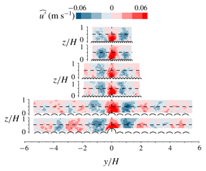
  $\widehat{u^{\prime }}$ contours. Nevertheless, the elongated streaks of alternating high and low momentum fluid with 2
 $H$ transverse period (figure 8) clearly indicate that VLSM are the key contributor to the ensemble average. Compared to the instantaneous velocity fluctuation fields reported in Cameron et al. (Reference Cameron, Nikora and Stewart2017), the
  $\widehat{u^{\prime }}$ fields are smoother and the meandering characteristic of the VLSM is suppressed due to the ensemble averaging. The alternating streaks for the high protrusion Delrin (‘D’) particles appear to be better defined compared to the low protrusion Nylon (‘N’) cases. This effect may reflect the observation that VLSM contribute less to the particle drag force (and therefore entrainment) as the protrusion is reduced (figure 1a) and the higher frequency pressure fluctuations due to the passage of smaller scale structures become relatively more important (Cameron et al. Reference Cameron, Nikora and Marusic2019).

Figure 8. Ensemble average of streamwise velocity fluctuation at  $z/H=0.5$ at time of entrainment. Mobile particle is at
  $x_{\ast }/H=0$,
  $y/H=0$.

Figure 9. Ensemble average of streamwise velocity fluctuation in the transverse plane at time of entrainment (a), and depth averaged velocity fluctuation at time of entrainment (b).

Figure 10. Ensemble average of streamwise velocity fluctuation in the streamwise plane at time of entrainment. Flow is from left to right.
Figure 9(a) indicates that the VLSM occupy nearly the entire flow depth from the roughness tops to the water surface such that the transverse periodicity of the velocity fluctuation is preserved after depth averaging (figure 9b). Figure 9(b) indicates that the transverse wavelength of the fluctuations is close to 2 $H$ for H030, but narrows slightly as the flow depth is increased to H120. A similar shortening of the transverse wavelength of VLSM with increasing relative submergence was also noted in Cameron et al. (Reference Cameron, Nikora and Stewart2017), but the origin of the effect is not yet known. Figure 9(b) also shows the depth average of the ensemble averaged vertical velocity fluctuation. Although the vertical velocity component is quite small and therefore not as well resolved in the ensemble average as the streamwise velocity component, a clear downflow region aligned with particle is seen, with upflow regions to the sides aligned with the zones of low streamwise momentum. This result is consistent with the depth scale counter-rotating vortical structure of VLSM (e.g. Hutchins & Marusic Reference Hutchins and Marusic2007; Cameron et al. Reference Cameron, Nikora and Stewart2017).
Figure 10 shows that the  $\widehat{u^{\prime }}$ contours are inclined with respect to the bed. This inclination likely results from the mean shear stretching the flow features as they evolve. At the instant of entrainment the target particle is immersed in the high velocity region of the VLSM where the drag force is maximised. For H030 the VLSM appear longer in terms of flow depths compared to H070 and H120 consistent with the scaling noted in Cameron et al. (Reference Cameron, Nikora and Stewart2017).
The role of VLSM in the particle entrainment process identified in figures 8–10 is consistent with previous indications (Cameron et al. Reference Cameron, Nikora and Marusic2019) that they contribute significantly to drag force fluctuations. In general, we can identify two reasons why very large-scale structures are favoured. Firstly, the contribution of small-scale velocity fluctuations to the drag force are suppressed by averaging over the spatial domain with volume comparable to the particle volume. This is described by the gain function  $|T_{D_{u}}|$ (equation (1.1), figure 1b). Secondly, the minimum force event duration (
 $t_{c}$) to completely entrain a particle acts as an additional filter, suppressing the contribution of higher frequency drag force fluctuations. For example, with a
  $t_{c}$ of 0.1–0.2 s for ‘D’ particles (figure 7), the
  ${\approx}10~\text{Hz}$ drag force fluctuations (figure 1a) that relate to pressure spatial fluctuations in the overlying turbulent flow, likely contribute very little to particle entrainment. For the ‘N’ spheres, however, with a
  $t_{c}$ of
  ${\approx}0.05~\text{s}$, and reduced sensitivity of the drag force to VLSM at the lower protrusion (figure 1a), the
  ${\approx}10~\text{Hz}$ pressure spatial fluctuations may play a more important role. Further data are required, with direct measurements of turbulent pressure fluctuations to confirm their contribution to particle entrainment.
3.4 Instantaneous flow field
In addition to the ensemble average velocity fluctuation fields, we have explored the instantaneous fields for each of the 300 recorded entrainment events for evidence of smaller scale ‘coherent structures’ contributing to entrainment. At the studied Reynolds numbers, however, the instantaneous fields appear as a random collection of vortices with different scales and orientations. It appears unlikely that any particular structure of analytical value relevant to sediment transport could be extracted. This, however, might be reviewed when high resolution volumetric data become available.
4 Conclusions
The ensemble average of velocity fields corresponding to the instant of particle entrainment demonstrate that sediment transport is strongly linked to VLSM in the flow. In particular, entrainment of single spherical particles occurs when the high momentum region of a very large-scale motion overlays a particle. Pressure spatial fluctuations which lead to a  ${\approx}10~\text{Hz}$ peak in premultiplied drag force spectra may also contribute to particle entrainment. This is particularly true for particles with small protrusion which have reduced exposure to the VLSM. The contribution of small-scale velocity fluctuations is suppressed by a spatial averaging effect associated with the particle size. Furthermore, drag and lift force fluctuations need to persist for sufficient duration to completely entrain a particle from its resting cavity. This minimum event duration limits the contribution of high frequency force fluctuations to the entrainment process. A relative submergence effect is seen in entrainment rate data which indicates that particle stability increases with decreasing flow depth under constant shear velocity conditions. This effect is also seen in the drag force variance and likely relates to suppression of the large-scale turbulence due to the limited separation between flow depth and roughness length scales. Further data are required to extend these observations to a wider range of relative flow submergence and particle Reynolds number, and to ascertain the potential role of particle lift forces which is still unclear.
Acknowledgements
The study has been supported by two EPSRC/UK grants, ‘High-resolution numerical and experimental studies of turbulence-induced sediment erosion and near-bed transport’ (EP/G056404/1) and ‘Bed friction in rough-bed free-surface flows: a theoretical framework, roughness regimes, and quantification’ (EP/K041088/1). The authors are grateful to three anonymous reviewers and the Editor for constructive criticisms and helpful suggestions that improved the presentation of the material in the paper.
Declaration of interests
The authors report no conflict of interest.


