2.1 Overview

The case that we examine consists of an array of four plumes in a horizontally periodic and square domain of height $H$ and horizontal dimensions $2SH\times 2SH$, as shown in figure 1. Each diagonal pair of plumes is driven by sources of buoyancy on either the top or the bottom of the domain. The sources are located in the centre of each quadrant and each provides a positive buoyancy flux $F$. For sufficiently large $S$, the resulting steady state consists of a stable two-layer stratification with a step change in buoyancy that is determined by entrainment into the plumes. An equivalent case was described in terms of line and point sources by Baines & Turner (Reference Baines and Turner1969, p. 72).

Figure 2 displays a vertical slice through the instantaneous buoyancy field for $S=1$. The buoyancy structure produced by localised sources of buoyancy contrasts with the approximately uniform state that would be produced by the uniform heating and cooling of the horizontal boundaries for Rayleigh Bénard convection. In the lower layer above a heat source a turbulent plume develops, whose fluid penetrates the interface between the layers, before being entrained by the adjacent plumes.

Figure 2. The buoyancy field $b(x,z)$ over a vertical slice of the domain. The domain shown has a quadrant aspect ratio of $S=1$ and the slice intersects the vertical axis of two of the plumes. The black line denotes a buoyancy isosurface of zero and the two white lines denote buoyancy isosurfaces at $\pm 5.6$.

2.2 Governing equations

The equations of motion for the Boussinesq flow considered here are

(2.1)$$\begin{eqnarray}\displaystyle & \displaystyle {\displaystyle \frac{\unicode[STIX]{x2202}\boldsymbol{u}}{\unicode[STIX]{x2202}t}}+\boldsymbol{u}\boldsymbol{\cdot }\unicode[STIX]{x1D735}\boldsymbol{u}=-\unicode[STIX]{x1D735}p+b\,\boldsymbol{k}+\frac{1}{Re}\unicode[STIX]{x1D6FB}^{2}\boldsymbol{u}, & \displaystyle\end{eqnarray}$$

(2.2)$$\begin{eqnarray}\displaystyle & \displaystyle \unicode[STIX]{x1D735}\boldsymbol{\cdot }\boldsymbol{u}=0, & \displaystyle\end{eqnarray}$$

(2.3)$$\begin{eqnarray}\displaystyle & \displaystyle {\displaystyle \frac{\unicode[STIX]{x2202}b}{\unicode[STIX]{x2202}t}}+\boldsymbol{u}\boldsymbol{\cdot }\unicode[STIX]{x1D735}b=\frac{1}{Pe}\unicode[STIX]{x1D6FB}^{2}b, & \displaystyle\end{eqnarray}$$

in which the scales used to non-dimensionalise velocity $\boldsymbol{u}$, buoyancy $b$, kinematic pressure $p$, space $(x,y,z)$ and time $t$ are $F^{1/3}H^{-1/3}$, $F^{2/3}H^{-5/3}$, $F^{2/3}H^{-2/3}$, $H$ and $F^{-1/3}H^{4/3}$, respectively. The unit vector $\boldsymbol{k}$, points in the vertical direction. The Reynolds and Péclet numbers are $Re=F^{1/3}H^{2/3}/\unicode[STIX]{x1D708}$ and $Pe=F^{1/3}H^{2/3}/\unicode[STIX]{x1D705}$, respectively, for kinematic viscosity $\unicode[STIX]{x1D708}$ and thermal diffusivity $\unicode[STIX]{x1D705}$. In terms of dimensionless variables, the buoyancy flux supplied by each source is equal to unity. To estimate an integral time scale for this problem we divide the quadrant volume $H^{3}S^{2}$ by the volume flux $F^{1/3}H^{5/3}$, which results in a horizontal turnover time of $F^{-1/3}H^{4/3}S^{2}$.

2.3 Simulation details

We will compare theoretical predictions to the direct simulation of (2.1)–(2.3). The code we use employs a fourth-order finite volume discretisation, the details of which are documented in Craske & van Reeuwijk (Reference Craske and van Reeuwijk2015a). We simulate the medium of air, with a Prandtl number $Pr=\unicode[STIX]{x1D708}/\unicode[STIX]{x1D705}=0.71$ and consider flows with Reynolds number $Re=4185$, which corresponds to a Rayleigh number of $Pr\,Re^{2}=1.24\times 10^{7}$. On the horizontal (top and bottom) boundaries we apply a free-slip condition on the velocity and homogeneous Neumann conditions on the buoyancy field outside the circular sources. Inside the circular sources we impose an inhomogeneous Neumann condition on buoyancy to produce a constant flux. On the vertical boundaries (sides) of the domain we impose periodic boundary conditions on all dependent variables. The grid is Cartesian and uniformly spaced; hence the shape of the nominally circular sources is formed approximately using square cells to fill a disk of diameter $D=H/5$. The plumes are unforced and therefore nominally lazy at their source (Hunt & Kaye Reference Hunt and Kaye2005). This means that the plumes contract in the vicinity of the source (Fanneløp & Webber Reference Fanneløp and Webber2003), resulting in an effective radius that is significantly less than the physical source radius (see, e.g. the sources in figure 2). A summary of the simulation details is provided in table 1 and in appendix B we demonstrate the convergence of the results and investigate their sensitivity with respect to changes in the Reynolds number.

Table 1. Simulation details. All simulations were run at $Re=4185$, $Pe=2971$ and $DN_{x}/2SH=154$, where $DN_{x}/2SH$ is the number of cells that span the source diameter $D$ for quadrant aspect ratio $S$. The symbols in the leftmost column correspond to those used in figures hereafter.

2.4 Domain decomposition

We take statistics over quadrants that are centred on each source, as illustrated in figure 1. Unlike the statistics that can be obtained over the entire horizontal plane, the quadrant statistics are, in general, vertically asymmetric with respect to the interface and allow us to isolate the vertical evolution of each plume. In addition, it proves convenient to respect the symmetry of the problem by aligning the origin of the vertical coordinate $z$ with the interface, as shown in figure 1.

We define time-averaged integrals by integrating over diagonal pairs of quadrants $\unicode[STIX]{x1D6FA}_{S}(z)$, for which the flow is statistically equivalent (see, for example, the square shaded regions in figure 1), such that

(2.4)$$\begin{eqnarray}\langle \,f\rangle (z)\equiv \frac{1}{2T}\int _{0}^{T}\int \int _{\unicode[STIX]{x1D6FA}_{S}(z)}f(\boldsymbol{x},t)\,\text{d}x\,\text{d}y\,\text{d}t.\end{eqnarray}$$

The time $T$ over which the integrals were averaged was not less than 1 dimensionless horizontal turnover time $F^{1/3}H^{-4/3}S^{2}$. Whilst the factor of 1/2 in (2.4) means that $\langle \,f\rangle$ can be interpreted as an integral over a ‘single’ quadrant, we emphasise that (2.4) integrates information from a diagonal pair of quadrants, in which the flow has the same sense, as shown in figure 1.

We will use double angles to denote integrals over a volume of the domain,

(2.5)$$\begin{eqnarray}\langle \langle \,f\rangle \rangle _{a}^{b}\equiv \int _{a}^{b}\langle f\rangle (z)\,\text{d}z.\end{eqnarray}$$

Acknowledging that our use of $\langle \rangle$ and $\langle \langle \rangle \rangle$ to denote integrals rather than averages is not standard, we note that for this problem, in which we vary the aspect ratio, it proves convenient. For example, the constant area-integrated buoyancy flux at each plume source is independent of a domain’s aspect ratio, in contrast to the spatially averaged buoyancy flux, which is inversely proportional to the aspect ratio squared.

3.1 Observations

Convection above or below each source in figure 2 results in turbulent plumes that entrain, dilute and transport fluid between the layers and, in doing so, determine an approximately two-layer stratification of the surrounding environment (Baines & Turner Reference Baines and Turner1969). Buoyancy conservation indicates that in a statistically steady state, in which the ambient buoyancy in each layer does not change, the mean buoyancy in a plume at the level of the interface is approximately equal to the ambient buoyancy of the layer downstream. We will therefore refer to the resulting neutrally buoyant flow into the downstream layer as a turbulent jet (as can be seen in the top left and bottom right of figure 2). For discussion purposes we will focus on the quadrant containing a plume oriented in the positive vertical direction, as highlighted in figure 1, and will therefore refer to the plume as occupying the lower layer and the jet as occupying the upper layer. In spite of the terminology we employ, we can see in figure 1 that density anomalies persist within the jets, rendering their flow different from conventional uniform-density jets.

Figure 3. Quadrant integrals of the average (a) buoyancy (divided by $S^{2}$), (b) volume flux and (c) relative buoyancy flux, for aspect ratios $S=1/2,7/12,15/24,2/3,1$ and $4/3$, as indicated by the symbols. The plume occupies the lower half of the domain, as highlighted in figure 1.

Figure 3 indicates how quadrant integrals of buoyancy, volume flux and relative buoyancy flux vary in the vertical direction. Figure 3(a) shows that as the aspect ratio of the domain increases, the difference between the buoyancy of the lower and upper layer increases. The buoyancy profiles in figure 3(a) are slightly asymmetric due to the influence of the plume, whose mean buoyancy is non-zero, in the lower layer. The asymmetry is relatively weak because the volume occupied by the plume is small in comparison with that of the domain.

The vertical volume flux is zero when integrated over the entire domain, but non-zero when integrated over a single quadrant. By examining the behaviour of the vertical volume flux in a single quadrant, we can therefore identify the strength and structure of the large-scale circulation. For example, if the vertical volume flux $\langle w\rangle$ is increasing with height $z$ then, by continuity, fluid is being drawn in through the sides of the quadrant at that height $z$. If, on the other hand, the vertical volume flux is decreasing with height, then there is a net flow of fluid out of the quadrant through its sides.

The vertical volume flux for a single quadrant is plotted in figure 3(b). For the three smallest aspect ratios $S=1/2,7/12,15/24$, figure 3(b) shows that the volume flux increases in a quadrant above the source (located at $z=-0.5$ in figure 3), before decreasing in the upper layer. This indicates that fluid is drawn into the quadrant through the sides in the lower layer, transported vertically between the layers and subsequently transported out of the quadrant through the sides in the upper layer, as evidenced explicitly in figure 4(a), which displays the vertical derivative of the volume flux. From the perspective of the spatially averaged flow, the entrainment and convection driven by the plumes results in a single-cell large-scale circulation between the quadrants, and volume conservation implies that these processes are necessarily symmetric about the mid-plane $z=0$.

Figure 4. The vertical derivative of the quadrant volume flux $\langle w\rangle$, which is equal to the horizontal flow through the vertical sides of the quadrant. The flows on domains of aspect ratio $S=1/2,7/12,15/24$ are shown in (a) and do not contain any critical points. The flow on a domain of aspect ratio $S=2/3$ is shown in (b) and contains two critical points and therefore bidirectional flow through the vertical sides of the quadrant in the upper and lower half of the domain. Flows on domains of aspect ratio $S=1,4/3$ are shown in (c) and contain four critical points, indicating the presence of a tertiary circulation cell at the interface. Horizontal cross-sections of the velocity field are plotted for the $S=4/3$ case in figure 5, at the heights indicated by dashed lines in (c).

Figure 5. Horizontal slices through the time-averaged velocity field and the horizontal divergence $\langle \unicode[STIX]{x2202}_{x}u+\unicode[STIX]{x2202}_{y}v\rangle$ (displayed in text) at (a) $z=0.1$, (b) $z=0.3$, (c) $z=0.45$ for aspect ratio $S=4/3$. The locations of these slices are plotted as dashed lines in figure 4(c). Note that persistent large scale structures in the horizontal flow result in time-averaged velocity fields in diagonal pairs of quadrants that are not necessarily identical.

In a spatially averaged sense, a topological change in the flow between quadrants occurs when the aspect ratio increases to $2/3$. This can be identified from the emergence of two local maxima in $\langle w\rangle$, as seen in figure 3(b), and the bidirectional flow in the upper and lower halves of figure 4(b). At a local maximum in $\langle w\rangle$, the mean horizontal flow across the sides of the quadrant changes direction, from a net flow into the quadrant to a net flow out of the quadrant. The appearance of two additional maxima therefore indicates that secondary circulation cells have developed in each layer. Noting that secondary circulations might exist within, rather than between, each quadrant for $S\leqslant 15/24$, we conclude that $S>15/24$ entails a secondary circulation that engulfs more than half of a given layer.

The secondary circulation cells form due to entrainment into the turbulent jets. When the plumes are sufficiently far apart, a given jet entrains fluid in addition to that which is supplied by the plume; hence the flux of volume that leaves the quadrant where the jet impinges on the horizontal boundary of the domain exceeds the total volume entrained by the plumes in the neighbouring quadrants and the residual volume recirculates. The existence of secondary circulation cells is therefore an indication that the plumes are, to some extent, behaving independently. We will demonstrate in § 4.6, where we analyse the velocity profiles within the jet, that the residual volume flux is indeed driven by entrainment into the jet, rather than being sustained as a co-flow outside the jet, which is not assured by the information in figures 3 and 4.

The additional volume flux due to entrainment into the jet can be calculated using plume theory. We assume that the flow nominally behaves as a turbulent jet above the interface. More precisely, the flow is a forced plume, because figure 3(c) indicates a residual buoyancy flux in the flow above the interface, which diminishes with aspect ratio. The volume flux in the jet is equal to the volume flux in the plume at the interface plus the volume flux due to the subsequent entrainment into the jet,

(3.1)$$\begin{eqnarray}Q(z)=\underbrace{Q_{m}}_{\text{plume}}+\underbrace{\frac{6\unicode[STIX]{x1D6FC}\sqrt{\unicode[STIX]{x03C0}}}{5}M_{m}^{1/2}z}_{\text{jet}},\end{eqnarray}$$

where $\unicode[STIX]{x1D6FC}$ is the entrainment coefficient for a plume and we have explicitly accounted for the fact that the entrainment coefficient in plumes is approximately $5/3$ larger than it is in jets (van Reeuwijk & Craske Reference van Reeuwijk and Craske2015). Hereafter it proves convenient to label the distance from the plume source to the interface using the symbol $\unicode[STIX]{x1D701}$. Hence, the quantities $Q_{m}$ and $M_{m}$ in (3.1), corresponding to the volume flux and momentum flux in the plume at the interface, respectively, are

(3.2a,b)$$\begin{eqnarray}Q_{m}=\frac{6\unicode[STIX]{x1D6FC}}{5}\left(\frac{9\unicode[STIX]{x1D6FC}\unicode[STIX]{x03C0}^{2}}{10}\right)^{1/3}\unicode[STIX]{x1D701}^{5/3},\quad M_{m}=\unicode[STIX]{x03C0}^{1/3}\left(\frac{9\unicode[STIX]{x1D6FC}}{10}\right)^{2/3}\unicode[STIX]{x1D701}^{4/3}.\end{eqnarray}$$

Equations (3.2a) and (3.2b) assume that the local (lower layer) environment is unstratified; a stratification would result in values of $Q_{m}$ and $M_{m}$ less than those predicted by (3.2a) and (3.2b). A comparison of (3.1) at $z=0$ with (3.2a) indicates that the rate at which the jet entrains volume $Q(z=\unicode[STIX]{x1D701})-Q_{m}$ is equal to the total volume entrainment rate $Q_{m}$ of the plume. This property is a consequence of the observed ratio of $5/3$ between the entrainment coefficient in a plume compared with a jet (van Reeuwijk & Craske Reference van Reeuwijk and Craske2015). Consequently, for sufficiently large aspect ratios, the strength of the secondary circulation is equal to the strength of the primary circulation, as can be verified from figure 3(b), which shows that the maximum value of $\langle w\rangle$ is twice as large as its value at $z=0$ for $S=4/3$. The maximum volume flux in a quadrant results from entrainment into the plume in addition to fluid that will be re-entrained by the adjacent jet.

For the domains of relatively large aspect ratio, such as $S=1$ and $S=4/3$, figure 3(b) shows that a further bifurcation in the mean-flow structure occurs. The change corresponds to the emergence of a third, relatively weak, circulation cell, which can also be identified from the two additional critical points in $\langle w\rangle$, as shown in figures 3(b) and 4(c). The three circulation cells for $S=4/3$ can also be observed in the horizontal velocity fields shown in figure 5. The quadrants for which the integrals in figures 4 and 5 were calculated correspond to the bottom left and top right quadrants. Just above the interface, where $z=0.1$, there is a net inflow into the top left and bottom right quadrants and a net outflow from the top right quadrant. At $z=0.3$, the divergence is stronger and indicates that the flow entering or leaving a given quadrant has reversed in comparison with $z=0.1$. At $z=0.45$ the direction of flow entering and leaving each quadrant changes for a second time and corresponds to the primary circulation driven by entrainment into the plumes.

We close our analysis of the mean flow’s topology by noting a likely influence of free-slip velocity boundary conditions in determining the shape and extent of the circulation cells. Such boundary conditions are convenient in allowing one to focus exclusively on the flow that is naturally driven by the plumes, in the absence of the competing, and aspect ratio dependent, effects arising from wall friction. We recognise, however, that practical problems involving confined turbulent plumes necessarily involve wall friction, in addition to the phenomena on which we focus.

For domains of sufficiently large aspect ratio, mass conservation implies that the vertical flux of buoyancy, relative to the ambient buoyancy, $\langle wb\rangle -\langle w\rangle \langle b\rangle /S^{2}$ within a quadrant will be equal to unity in the layer containing the plume and zero in the layer containing the jet. This argument requires the ambient buoyancy in each layer to be uniform, such that the flux of buoyancy, relative to the ambient is zero. Figure 3(c) indicates that this is approximately correct for the two largest aspect ratios $S=1,4/3$, excepting a relatively small residual flux in the upper layer. In the vicinity of the top boundary at $z=1/2$, the relative buoyancy flux $\langle wb\rangle -\langle w\rangle \langle b\rangle /S^{2}$ reduces to zero and the buoyancy in figure 3(a) increases, which suggests that the residual buoyancy is transported out of the quadrant horizontally in a steady axisymmetric gravity current.

3.2 Entrainment

In general, flows driven by turbulent plumes are interpreted and modelled using plume theory and an entrainment coefficient, under the assumption that each plume acts independently. Entrainment can be estimated from observed volume fluxes or buoyancy differences. In this section we will calculate effective entrainment coefficients $\unicode[STIX]{x1D6FC}_{\ast }$ from observations of volume flux and buoyancy, and use the estimates to identify aspect ratios for which plume theory provides a faithful description of the flow.

In the context of plume theory, the increase in the volume flux in a plume is equal to the rate of entrainment from the surrounding environment. Entrainment is typically parameterised as being proportional to the square root of the momentum flux in the flow, as discussed in Baines & Turner (Reference Baines and Turner1969). The resulting coefficient of proportionality for an isolated unconfined plume is $\unicode[STIX]{x1D6FC}\approx 0.12$ (Carazzo, Kaminski & Tait Reference Carazzo, Kaminski and Tait2006; van Reeuwijk & Craske Reference van Reeuwijk and Craske2015).

Following Baines & Turner (Reference Baines and Turner1969), there are two ways to calculate an entrainment coefficient from the observations reported here. One method is to find the entrainment coefficient from the volume flux at the mid-plane. This could be considered the ab initio estimation of entrainment, because it describes the rate of increase of the volume flux in the plume directly. Alternatively, we can calculate the entrainment coefficient that would be required to predict the observed difference in buoyancy between the upper and lower layers under the assumption that mixing occurs exclusively within the plumes. If the two entrainment rates are equal, they suggest that plume theory provides a faithful description of the flow.

For transparency, we refrain from using a virtual source (Hunt & Kaye Reference Hunt and Kaye2001) to account for the finite area of the sources used in the simulations. Indeed, the theoretical location of the virtual source of the infinitely lazy plumes (zero source momentum flux) in this problem coincide with the vertical location of the actual sources, i.e. the theoretical virtual source correction is zero (Hunt & Kaye Reference Hunt and Kaye2001). However, figure 2 suggests that, unlike the idealised contraction of lazy plumes that is predicted by plume theory, the near-field behaviour of the plumes in this study is disrupted by background turbulence; hence the use of an effective virtual source might be appropriate. We therefore note that by proceeding without using a virtual source, which would increase $\unicode[STIX]{x1D701}$ (the distance between the plume source and the interface) in (3.3) and (3.5) below, our estimations of the entrainment coefficient are likely to be slightly larger than they would be if a virtual source were incorporated.

First we will calculate an effective entrainment coefficient from the volume flux at the interface. Inverting (3.2a) provides a means of estimating the entrainment coefficient from observations of the volume flux at the interface,

(3.3)$$\begin{eqnarray}\unicode[STIX]{x1D6FC}_{Q}=\left(\frac{5}{6}\right)^{3/4}\left(\frac{10}{9\unicode[STIX]{x03C0}^{2}}\right)^{1/4}\frac{Q_{m}^{3/4}}{\unicode[STIX]{x1D701}^{5/4}},\end{eqnarray}$$

where $\unicode[STIX]{x1D701}$ is the distance from the plume source to the interface and $Q_{m}$ is the volume flux at the level of the interface (plotted in figure 6(a)). The entrainment coefficient estimated from (3.3) is plotted against the aspect ratio $S$ in figure 6(c) (solid line).

Figure 6. An effective entrainment coefficient using plume theory: (a) the volume flux at the interface $Q_{m}$, (b) half the difference in buoyancy between the layers $b_{m}$ and (c) the effective entrainment coefficient $\unicode[STIX]{x1D6FC}_{\ast }$ for various aspect ratios $S$ (see table 1). An estimate for the entrainment rate $\unicode[STIX]{x1D6FC}_{Q}$ (solid line) can be calculated from $Q_{m}$ and (3.3). A second estimate for the entrainment coefficient $\unicode[STIX]{x1D6FC}_{b}$ (dashed line) is the value required to explain the observed buoyancy difference $b_{m}$ between the layers (3.5).

From figure 6(c) we see that the entrainment coefficient, $\unicode[STIX]{x1D6FC}_{Q}$, calculated from the volume flux at the interface $Q_{m}$, increases with aspect ratio $S$ up to some critical aspect ratio of approximately $S\approx 2/3$. Interestingly, this is close to the aspect ratio for which we observed a topological change in the mean flow between quadrants and the emergence of the secondary circulation cells in the upper and lower layers (cf. § 3.1). As (3.3) assumes an unstratified ambient, the increase in the estimate of $\unicode[STIX]{x1D6FC}_{Q}$ with increasing aspect ratio $S$ at low aspect ratios may be due to the reduction of the stratification in the lower layer as the aspect ratio increases. Increasing the aspect ratio further results in a reduction in the entrainment coefficient, which appears to be tending towards a value that is slightly higher than the value of $0.12$ that is commonly associated with an isolated plume in an unconfined environment.

A second method for calculating an effective entrainment coefficient is from the difference in buoyancy between the layers. In a steady state, mass conservation implies that the buoyancy of a given layer is approximately equal to the mean buoyancy $\pm b_{m}$ of the plume supplying fluid to that layer. We define the relative buoyancy flux in each plume as being equal to the volume flux $Q$ multiplied by the buoyancy of the plume relative to the buoyancy of the local environment. The buoyancy flux of a plume just beneath the interface is therefore $Q_{m}(b_{m}-(-b_{m}))=2Q_{m}b_{m}$. Assuming an unstratified environment in each layer, the buoyancy flux in the plume must be equal to the dimensionless source buoyancy flux, therefore $2Q_{m}b_{m}=1$, which implies that $b_{m}=1/(2Q_{m})$.

Noting that $b_{m}=1/(2Q_{m})$ and considering (3.2a), the buoyancy of the upper layer should obey

(3.4)$$\begin{eqnarray}b_{m}=\frac{5}{12\unicode[STIX]{x1D6FC}}\left(\frac{10}{9\unicode[STIX]{x1D6FC}\unicode[STIX]{x03C0}^{2}}\right)^{1/3}\frac{1}{\unicode[STIX]{x1D701}^{5/3}}.\end{eqnarray}$$

Strictly, the relationship (3.4) between the buoyancy of a layer and the mean buoyancy of the plume by which it is fed is approximate because a small proportion of the plume’s total buoyancy flux is provided by turbulent transport, which is formally independent of the mean buoyancy in the plume. In other words, the actual relative buoyancy flux in the plume just beneath the interface is $2Q_{m}b_{m}$ plus a contribution of approximately 15 % from turbulent transport (van Reeuwijk et al. Reference van Reeuwijk, Salizzoni, Hunt and Craske2016). Consequently, the buoyancy of a given layer is typically slightly greater in magnitude than the mean buoyancy of the plume might suggest.

We determine $b_{m}$ as half the distance between peaks in the time-averaged probability density function for buoyancy, which is shown in figure 7 and will be discussed in § 4.1. The value of $b_{m}$ for each value of $S$ is plotted in figure 6(b). Knowledge of $b_{m}$ and use of (3.4) means that the entrainment coefficient can be estimated independently of (3.3) from

(3.5)$$\begin{eqnarray}\unicode[STIX]{x1D6FC}_{b}=\left(\frac{5}{12}\right)^{3/4}\left(\frac{10}{9\unicode[STIX]{x03C0}^{2}}\right)^{1/4}\frac{1}{b_{m}^{3/4}\unicode[STIX]{x1D701}^{5/4}}.\end{eqnarray}$$

The entrainment coefficient as calculated from (3.5) is plotted in figure 6(c) (dashed line). This entrainment rate can be considered as the entrainment rate required as input into a plume model to explain the observed buoyancy difference between the layers.

We observe from figure 6(c), that the entrainment coefficient calculated from $b_{m}$, using (3.5), results in a value of $\unicode[STIX]{x1D6FC}_{b}$ that is everywhere greater than the value of $\unicode[STIX]{x1D6FC}\approx 0.12$ that is commonly assigned to isolated and unconfined plumes. Indeed, the use of $\unicode[STIX]{x1D6FC}\approx 0.12$ would significantly overestimate the buoyancy difference between the upper and lower layers. Figure 6(c) shows that calculating an entrainment coefficient from the buoyancy field using (3.5), results in a larger estimate for $\unicode[STIX]{x1D6FC}$ than (3.3), which is based on the volume flux. The difference can be attributed to two distinct effects. First, the estimation (3.5) implicitly assumes that vertical buoyancy transport can be assigned exclusively to the plumes, rather than interfacial mixing. Secondly, equation (3.3) does not account for stratification within each layer, which is significant for domains with relatively small aspect ratio and would lead to an increase in the corresponding prediction of $\unicode[STIX]{x1D6FC}_{b}$ and a decrease in the predictions of $\unicode[STIX]{x1D6FC}_{Q}$.

Figure 7. The time-averaged probability density function of the buoyancy, which corresponds to $\unicode[STIX]{x2202}z_{\ast }/\unicode[STIX]{x2202}b$, over the entire domain for different aspect ratios.

Figure 6 indicates that for $S=4/3$ equations (3.3) and (3.5) provide almost identical and therefore robust estimates for $\unicode[STIX]{x1D6FC}$, which suggests that the effects of interfacial mixing are insignificant for $S\geqslant 4/3$. However, the estimated value $\unicode[STIX]{x1D6FC}_{\ast }\approx 0.2$ for $S=4/3$ is larger than $\unicode[STIX]{x1D6FC}\approx 0.12$ for an isolated plume in an unconfined domain. In this regard, the use of an effective virtual source, a distance $\unicode[STIX]{x1D706}\unicode[STIX]{x1D701}$ further from the interface than the actual source, would lead to an estimate of $\unicode[STIX]{x1D6FC}_{\ast }\approx 0.2/(1+\unicode[STIX]{x1D706})^{5/4}$. However, noting that classical plume theory predicts the virtual source correction for infinitely lazy plumes to be zero (Hunt & Kaye Reference Hunt and Kaye2001), we would associate an effective virtual source with the indirect effect that background turbulence has in modifying the near-field development of the plume. In view of the reduction in entrainment with respect to background turbulence reported by (Khorsandi et al. Reference Khorsandi, Gaskin and Mydlarski2013; Lai et al. Reference Lai, Law and Adams2019), attribution of $\unicode[STIX]{x1D6FC}_{\ast }=0.2$ solely to direct effects of background turbulence would therefore be incorrect and misleading, not least because it would also ignore possible modifications to entrainment arising from the mean ambient flow discussed in § 3.

We conclude by noting that the quadrant aspect ratios $S=1,4/3$ approximately correspond to the critical aspect ratio $H/R=1$ for overturning identified by Baines & Turner (Reference Baines and Turner1969), if the radius $R$ of the cylinder containing their single plume is compared with the shortest distance $SH$ between the plume axes of the present problem.

4.1 Governing equations for energetics

Let $z_{\ast }(b,t)$ represent an adiabatic rearrangement of the fluid into the configuration possessing the minimal potential energy and, therefore, a monotonically increasing reference buoyancy $b_{\ast }(z,t)$. The minimal potential energy is equal to the BPE (Lorenz Reference Lorenz1955). For this problem, in which $z_{\ast }\in [-0.5,0.5]$, the quantity $\unicode[STIX]{x2202}z_{\ast }/\unicode[STIX]{x2202}b$ corresponds to the probability density function for buoyancy. Indeed, $z_{\ast }$ can be obtained during a simulation by integrating the probability density function for buoyancy (Winters et al. Reference Winters, Lombard, Riley and D’Asaro1995). The histograms of the time average of $\unicode[STIX]{x2202}z_{\ast }/\unicode[STIX]{x2202}b$ for different aspect ratios shown in figure 7 demonstrate that as the domain aspect ratio increases the variance of the global distribution of buoyancy increases.

When non-dimensionalised, the local gravitational potential energy of the fluid is $E_{p}\equiv -bz$. Typically, the portion of the potential energy that is available to do work to increase the kinetic energy of the flow is computed as the volume integral of $b(z_{\ast }-z)$ (Winters et al. Reference Winters, Lombard, Riley and D’Asaro1995). Locally, however, $b(z_{\ast }-z)$ is not positive definite, which motivates the definition of a suitable local APE density. Following Holliday & Mcintyre (Reference Holliday and Mcintyre1981) and Scotti & White (Reference Scotti and White2014), we therefore consider the positive semidefinite quantity

(4.1)$$\begin{eqnarray}E_{a}\equiv \int _{b_{\ast }}^{b}(z_{\ast }(\hat{b},t)-z)\,\text{d}\hat{b}.\end{eqnarray}$$

Physically, the definition (4.1) is positive semidefinite because it accounts for both the potential energy associated with a parcel of fluid displaced from equilibrium and the potential energy associated with the corresponding displacement of the environment, as can be seen by decomposing (4.1),

(4.2)$$\begin{eqnarray}E_{a}=b(z_{\ast }-z)-\int _{0}^{z-z_{\ast }}b_{\ast }(z-\hat{z},t)\,\text{d}\hat{z},\end{eqnarray}$$

where $b_{\ast }(z,t)$ is the reference buoyancy, such that $z_{\ast }(b_{\ast }(z,t),t)=z$, corresponding to the adiabatically rearranged state possessing minimal potential energy. The quantity $E_{a}$ therefore has a dependence on the structure of the entire buoyancy field, i.e. the value of $E_{a}$ at a point may change because parcels of fluid mixing at locations that are remote from that point leads to a modification of $b_{\ast }$. In the problem that we consider the reference buoyancy can be equated with the ambient buoyancy $\pm b_{m}$, except over thin layers at the bottom, middle and top of the domain. Using (2.3), the Lagrangian derivative of $E_{a}$ satisfies (Scotti & White Reference Scotti and White2014)

(4.3)$$\begin{eqnarray}{\displaystyle \frac{\text{D}E_{a}}{\text{D}t}}=\frac{\unicode[STIX]{x1D6FB}^{2}E_{a}}{Pe}+\frac{2}{Pe}\frac{\unicode[STIX]{x2202}(b-b_{\ast })}{\unicode[STIX]{x2202}z}-G-w(b-b_{\ast })+\int _{b_{\ast }}^{b}w_{\ast }(\hat{b},t)\,\text{d}\hat{b},\end{eqnarray}$$

where the APE dissipation

(4.4a,b)$$\begin{eqnarray}G\equiv \frac{1}{Pe}\left(|\unicode[STIX]{x1D735}b|^{2}\left.\frac{\unicode[STIX]{x2202}z_{\ast }}{\unicode[STIX]{x2202}b}\right|_{b}-|\unicode[STIX]{x1D735}b_{\ast }|^{2}\left.\frac{\unicode[STIX]{x2202}z_{\ast }}{\unicode[STIX]{x2202}b}\right|_{b_{\ast }}\right),\quad \text{and}\quad w_{\ast }\equiv {\displaystyle \frac{\unicode[STIX]{x2202}z_{\ast }}{\unicode[STIX]{x2202}t}}.\end{eqnarray}$$

The final term in (4.3) is zero when the probability density function for buoyancy (cf. figure 7) does not depend on time, which is true in the present context for domains that are of sufficiently large aspect ratio. In that case, equation (4.3) reduces to

(4.5)$$\begin{eqnarray}{\displaystyle \frac{\unicode[STIX]{x2202}E_{a}}{\unicode[STIX]{x2202}t}}+\unicode[STIX]{x1D735}\boldsymbol{\cdot }(\boldsymbol{u}E_{a})=\frac{\unicode[STIX]{x1D6FB}^{2}E_{a}}{Pe}+\frac{2}{Pe}{\displaystyle \frac{\unicode[STIX]{x2202}(b-b_{\ast })}{\unicode[STIX]{x2202}z}}-G-\underbrace{w(b-b_{\ast })}_{-\unicode[STIX]{x1D6F7}_{z}},\end{eqnarray}$$

in which $-\unicode[STIX]{x1D6F7}_{z}$ is a buoyancy flux relative to the reference state.

Following Scotti & White (Reference Scotti and White2014), we define the local BPE density $E_{b}$ as $E_{b}\equiv -bz-E_{a}$, whose budget obeys

(4.6)$$\begin{eqnarray}{\displaystyle \frac{\unicode[STIX]{x2202}E_{b}}{\unicode[STIX]{x2202}t}}+\unicode[STIX]{x1D735}\boldsymbol{\cdot }(\boldsymbol{u}E_{b})=\frac{\unicode[STIX]{x1D6FB}^{2}\unicode[STIX]{x1D713}}{Pe}-\unicode[STIX]{x1D735}\boldsymbol{\cdot }(\boldsymbol{u}p_{\ast })+\underbrace{\left.\frac{|\unicode[STIX]{x1D735}b|^{2}}{Pe}{\displaystyle \frac{\unicode[STIX]{x2202}z_{\ast }}{\unicode[STIX]{x2202}b}}\right|_{b}}_{\unicode[STIX]{x1D6F7}_{d}},\end{eqnarray}$$

where

(4.7a,b)$$\begin{eqnarray}\unicode[STIX]{x1D713}=-\int _{0}^{b}z_{\ast }(\hat{b})\,\text{d}\hat{b},\quad p_{\ast }=\int _{0}^{z}b_{\ast }(\hat{z})\,\text{d}\hat{z}.\end{eqnarray}$$

In a Boussinesq flow, the mixing rate $\unicode[STIX]{x1D6F7}_{d}$ represents an irreversible conversion of APE into BPE via diapycnal mixing. An interesting feature of $\unicode[STIX]{x1D6F7}_{d}$, which proves to be crucial when considering energetics and entrainment, is that it corresponds to the dissipation of buoyancy variance $|\unicode[STIX]{x1D735}b|^{2}/Pe$ weighted by the probability density function $\unicode[STIX]{x2202}_{b}z_{\ast }$. Diapycnal mixing therefore has more energetic significance when it accounts for mixing in regions of buoyancy whose probability density is relatively large.

In the subsequent analysis, we choose to focus on the production of BPE $\unicode[STIX]{x1D6F7}_{d}$ rather than the APE dissipation $G$, because it is the volume integral of $\unicode[STIX]{x1D6F7}_{d}$ that features explicitly in previous work on bulk energetics (Winters et al. Reference Winters, Lombard, Riley and D’Asaro1995; Hughes et al. Reference Hughes, Gayen and Griffiths2013, for example) and evaluates to unity in this particular problem (see (4.11)). We note that locally BPE production, $\unicode[STIX]{x1D6F7}_{d}$, is not necessarily equal to APE dissipation $G$, because the latter only accounts for mixing resulting from macroscopic motion in the flow and not the mixing $(\unicode[STIX]{x2202}z_{\ast }/\unicode[STIX]{x2202}b)|\unicode[STIX]{x1D735}b_{\ast }|^{2}/Pe$ associated with diffusion of the background state; hence $\unicode[STIX]{x1D6F7}_{d}\geqslant G$ for the Boussinesq model considered here. However, in the present problem, the rearranged state consists primarily of two constant-density layers in which $\unicode[STIX]{x1D735}b_{\ast }\approx 0$ (see, for example, figure 7). With the possible exception of thin layers near the horizontal boundaries, $\unicode[STIX]{x1D6F7}_{d}$ and $G$ are therefore approximately equal, because they are dominated by the large gradients of $b$ within the plumes. In regarding local BPE production as equivalent to APE dissipation for this particular Boussinesq flow we are not endorsing the use of BPE production to characterise mixing more generally. The energy conversion implied by BPE production is different to APE dissipation (Tailleux Reference Tailleux2009) and in non-Boussinesq models, for which BPE ‘production’ can be negative (Tailleux Reference Tailleux2009; Gregg et al. Reference Gregg, D’Asaro, Riley and Kunze2018), the difference is significant.

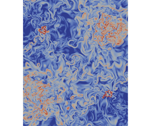
Figure 8. The BPE production $\unicode[STIX]{x1D6F7}_{d}=(\text{d}z_{\ast }/\text{d}b)|\unicode[STIX]{x1D735}\,b|^{2}/Pe$ over a vertical slice of the domain using a logarithmic scale. The domain has a quadrant aspect ratio of $S=1$ and the slice intersects the vertical axis of two of the plumes. The slice was taken at the same time as that of the buoyancy field displayed in figure 2.

The BPE production over vertical and horizontal slices is displayed in figures 8 and 9, respectively. These figures illustrate that regions of high $\unicode[STIX]{x1D6F7}_{d}$ typically occur on thin surfaces at the instantaneous edge of the plumes (cf. figure 2, corresponding to the same point in time), where both $|\unicode[STIX]{x1D735}b|$ and the probability density $\unicode[STIX]{x2202}z_{\ast }/\unicode[STIX]{x2202}b$ are relatively large because the buoyancy is close to a background buoyancy $\pm b_{m}$. Diapycnal mixing is energetically insignificant in the vicinity of the interface outside the plumes for the aspect ratio $S=1$ shown in figure 8, although the instantaneous picture of figure 8 does not necessarily account for intermittent events that would increase the mean BPE production.

Figure 9. The BPE production $\unicode[STIX]{x1D6F7}_{d}=(\text{d}z_{\ast }/\text{d}b)|\unicode[STIX]{x1D735}\,b|^{2}/Pe$ over horizontal slices of the domain using a logarithmic scale. The slices were taken at $z=0,0.1,0.2,0.45$ clockwise from top left. The plumes in each slice can be seen in the top-left and bottom-right quadrants of each window and the jets in the bottom-left and top-right quadrants. For the colour scale used in the figure see figure 8.

The local kinetic energy density $E_{k}$ (per unit mass) is defined according to $E_{k}\equiv |\boldsymbol{u}|^{2}/2$, and satisfies

(4.8)$$\begin{eqnarray}{\displaystyle \frac{\unicode[STIX]{x2202}E_{k}}{\unicode[STIX]{x2202}t}}+\unicode[STIX]{x1D735}\boldsymbol{\cdot }(\boldsymbol{u}E_{k})=-\unicode[STIX]{x1D735}\boldsymbol{\cdot }(\boldsymbol{u}(p-p_{\ast }))+\underbrace{w(b-b_{\ast })}_{-\unicode[STIX]{x1D6F7}_{z}}+\frac{1}{Re}\unicode[STIX]{x1D6FB}^{2}E_{k}-\unicode[STIX]{x1D700}.\end{eqnarray}$$

We will refer to the term $\unicode[STIX]{x1D700}\equiv (\unicode[STIX]{x2202}_{j}u_{i})^{2}/Re$ as the viscous dissipation, noting that, prior to spatial integration, the time average of $\unicode[STIX]{x1D700}$ is strictly only equivalent to the true viscous dissipation at a given point in homogeneous turbulence. The physical role played by the relative buoyancy flux $-\unicode[STIX]{x1D6F7}_{z}$ in (4.5) and (4.8) is the reversible conversion of APE into kinetic energy (Winters et al. Reference Winters, Lombard, Riley and D’Asaro1995).

The viscous dissipation $\unicode[STIX]{x1D700}$ of kinetic energy in (4.8) depends exclusively on local quantities, in the sense that it is evaluated from properties of the velocity field at a single point. In contrast, the BPE production $\unicode[STIX]{x1D6F7}_{d}$ (and APE dissipation) depends explicitly on the global probability density function for buoyancy. As illustrated in figure 10, $\unicode[STIX]{x1D700}$ is relatively large in the core of the plume, which is enveloped by surfaces on which $\unicode[STIX]{x1D6F7}_{d}$ is maximised. Such surfaces correspond to relatively large values of both $|\unicode[STIX]{x1D735}b|$ and the probability density function for buoyancy (i.e. surfaces on which $b\approx \pm b_{m}$, corresponding approximately to the the white lines in figure 2).

Figure 10. Regions of viscous dissipation $\unicode[STIX]{x1D700}=(\unicode[STIX]{x2202}_{j}u_{i})^{2}/Re$ coloured using a logarithmic scale. The thin dark (blue) parts of the figure denotes regions in which the BPE production $\unicode[STIX]{x1D6F7}_{d}=\text{d}z_{\ast }/\text{d}b|\unicode[STIX]{x1D735}\,b|^{2}/Pe\geqslant 3$.

Table 2. Domain decomposition of the buoyancy flux $\langle \langle \unicode[STIX]{x1D6F7}_{z}\rangle \rangle$, viscous dissipation $\langle \langle \unicode[STIX]{x1D700}\rangle \rangle$ and BPE production $\langle \langle \unicode[STIX]{x1D6F7}_{d}\rangle \rangle$; $\langle \langle \rangle \rangle ,\langle \langle \rangle \rangle _{-\unicode[STIX]{x1D701}}^{0}$ and $\langle \langle \rangle \rangle _{0}^{\unicode[STIX]{x1D701}}$ refer to volume integrals over an entire quadrant, the (lower) plume layer and the (upper) jet layer, respectively. The row labelled ‘Theory’ corresponds to the results obtained for Gaussian profiles in §§ 4.3 and 4.4. Noting that each layer of the domain has height $0.5$, the volume integrals displayed in this table have been multiplied by a factor of $2$, to facilitate a comparison with the horizontal axis of figure 11 and the interpretation of their ratios.

4.2 Integrals and statistics for energetics

The quadrant volume integrals of $\unicode[STIX]{x1D6F7}_{z}$, $\unicode[STIX]{x1D700}$ and $\unicode[STIX]{x1D6F7}_{d}$, multiplied by a factor of $2$, are displayed in table 2. The factor of $2$ was introduced to ensure that the theoretical predictions of $\unicode[STIX]{x1D6F7}_{z}$, $\unicode[STIX]{x1D700}$ and $\unicode[STIX]{x1D6F7}_{d}$ each correspond to unity. The values indicate that, whilst substantially more BPE production takes place in the lower layer than in the upper layer, the distribution of viscous dissipation in each of the quadrant’s layers is approximately uniform.

Integration of (4.8) over the volume of a quadrant and time, indicates that the integral of viscous dissipation is equal to the work done by buoyancy,

(4.9)$$\begin{eqnarray}\langle \langle \unicode[STIX]{x1D700}\rangle \rangle =-\langle \langle \unicode[STIX]{x1D6F7}_{z}\rangle \rangle ,\end{eqnarray}$$

where $\langle \langle \unicode[STIX]{x1D6F7}_{z}\rangle \rangle =-\langle \langle w(b-b_{\ast })\rangle \rangle =-\langle \langle wb\rangle \rangle$, because $b_{\ast }$ does not depend on $x$ or $y$ and therefore $\langle \langle wb_{\ast }\rangle \rangle$ is identically zero. It is interesting that for the two largest aspect ratios $\langle \langle \unicode[STIX]{x1D6F7}_{z}\rangle \rangle$ is greater than $1$, which exceeds the buoyancy flux provided by the sources. The cause of the disparity is seen when the governing equation for buoyancy (2.3) is multiplied by $z$ to give a volumetric budget for the potential energy $E_{a}+E_{b}=-bz$, which implies that

(4.10)$$\begin{eqnarray}-\langle \langle \unicode[STIX]{x1D6F7}_{z}\rangle \rangle -\langle \langle \unicode[STIX]{x1D6F7}_{i}\rangle \rangle =\underbrace{-\frac{1}{Pe}\left\langle {\displaystyle \frac{\unicode[STIX]{x2202}b}{\unicode[STIX]{x2202}z}}z\right\rangle _{-\unicode[STIX]{x1D701}}^{\unicode[STIX]{x1D701}}}_{=1/2},\end{eqnarray}$$

over a single quadrant. The right-hand side of (4.10) is equal to 1/2 because a given quadrant contains a single source of buoyancy at either $z=-1/2$ or $z=1/2$. The input of potential energy at the boundaries is therefore equal to the sum of the integral of the convective buoyancy flux and diffusion of buoyancy down its mean profile $-\langle \langle \unicode[STIX]{x1D6F7}_{i}\rangle \rangle \equiv -\langle \langle Pe^{-1}\unicode[STIX]{x2202}_{z}b\rangle \rangle$. Indeed, there is a flux of buoyancy due to the plume in addition to a (negative) diffusive flux down the stable background stratification. Together, these contributions result in $\langle \langle \unicode[STIX]{x1D6F7}_{z}\rangle \rangle$ being either slightly higher or slightly lower than the input at the boundaries, depending on the area of the plume sources, relative to the area of the horizontal boundaries. Nevertheless, the contribution from $\langle \langle \unicode[STIX]{x1D6F7}_{i}\rangle \rangle$ is small relative to the buoyancy flux $\langle \langle \unicode[STIX]{x1D6F7}_{z}\rangle \rangle$, due to the relatively high Péclet number of the flow, which results in a close agreement between $-\langle \langle \unicode[STIX]{x1D6F7}_{z}\rangle \rangle$ and the surface buoyancy fluxes in (4.10).

Unlike the viscous dissipation, which relies on the conversion of APE to kinetic energy via $\langle \langle \unicode[STIX]{x1D6F7}_{z}\rangle \rangle$, the volumetric production of BPE can be calculated directly from surface fluxes,

(4.11)$$\begin{eqnarray}\langle \langle \unicode[STIX]{x1D6F7}_{d}\rangle \rangle =\underbrace{\frac{1}{Pe}\left\langle {\displaystyle \frac{\unicode[STIX]{x2202}b}{\unicode[STIX]{x2202}z}}z_{\ast }\right\rangle _{-\unicode[STIX]{x1D701}}^{\unicode[STIX]{x1D701}}}_{=1/2},\end{eqnarray}$$

for sufficiently long time averages, as is verified to within approximately 1 % by the values (scaled by a factor of $2$) in table 2. The data in table 2 also show that the total input of APE at the boundaries, which is equal to twice the input of potential energy, is split equally between BPE production and viscous dissipation, leading to the mixing efficiency of approximately 1/2 that is also found in Rayleigh–Bénard convection (Hughes et al. Reference Hughes, Gayen and Griffiths2013).

Table 2 indicates that the viscous dissipation in the lower layer $\langle \langle \unicode[STIX]{x1D700}\rangle \rangle _{-\unicode[STIX]{x1D701}}^{0}$ generally decreases with increasing aspect ratio. In general, and particularly in domains of small aspect ratio, turbulence is transported horizontally out of a quadrant’s upper layer (which, for the purpose of discussion, we assume contains the jet) and into neighbouring quadrants. At larger aspect ratios a greater proportion of this turbulence is dissipated before it is transported out of the upper layer, leading to the observed decrease in lower-layer viscous dissipation for large aspect ratios.

Figure 11. (a) BPE production and (b) viscous dissipation over a quadrant of the domain. In this quadrant the plume occupies the lower layer and the jet occupies the upper layer. The thick (red) lines correspond to the theoretical predictions. The model in (a) is developed in § 4.5. The model is dashed in regions close to the source, because it was developed under the assumption of point sources of buoyancy flux. The thick line in (b) is the total dissipation in the lower layer (4.13), divided by the layer height, which gives $\langle \unicode[STIX]{x1D700}\rangle =1/2$ for a Gaussian velocity profile. The dashed line in (b) is described by (4.14) and corresponds to viscous dissipation in an unconfined jet. For the symbols used to denote each aspect ratio see table 1.

Figure 11 displays horizontal integrals of (a) the BPE production $\langle \unicode[STIX]{x1D6F7}_{d}\rangle$ and (b) the viscous dissipation $\langle \unicode[STIX]{x1D700}\rangle$ over the quadrant as a function of $z$. Consistent with the information in table 2, figure 11 indicates that the BPE production is significantly higher in the plume below the interface than it is in the jet above the interface, in which it decays with respect to $z$. In the lower layer the BPE production exhibits a local maximum of approximately $0.8$ for the largest aspect ratio. Due to the finite area of the source, the production of BPE production increases significantly in the vicinity of the bottom boundary. In the following sections we develop the integral model whose predictions are compared to the observations in figure 11.

4.3 Viscous dissipation

In this section we will develop a bulk model for the volume integral of viscous dissipation $\langle \langle \unicode[STIX]{x1D700}\rangle \rangle$ in the quadrant layer that contains a jet and the quadrant layer that contains a plume. We will also describe a model for the vertical variation of horizontally integrated viscous dissipation in each layer.

For generality we will assume that the distance from the plume source to the interface is $0\leqslant \unicode[STIX]{x1D701}\leqslant 1$, and not necessarily equal to 1/2. In practice, the situation we have in mind might correspond to an ‘emptying filling box’ model of a space ventilated by low and high-level openings (Linden et al. Reference Linden, Lane-Serff and Smeed1990) or to a domain containing an unequal number of buoyancy sources on its bottom boundary compared with its top boundary. For consistency with the previous sections, we continue to regard the ambient buoyancy of the upper layer as $b_{m}$ and that of the lower layer as $-b_{m}$.

In the absence of a direct input of kinetic energy at the boundaries, the viscous dissipation in the domain is balanced by the total work undertaken by buoyancy. Buoyancy is only able to do work on the flow in the quadrant’s lower layer ($z<0$), because in the upper layer the mean buoyancy difference between the plume and the ambient is zero. As discussed in § 4.2, provided that the vertical buoyancy transport by diffusion is small compared with the relative buoyancy flux $w(b-b_{\ast })$, the kinetic energy dissipation is equal to the buoyancy flux multiplied by $\unicode[STIX]{x1D701}$, which is the dimensionless distance over which buoyancy is able to do work in a single quadrant.

Assuming that the aspect ratio is sufficiently large and that the upper layer is not stratified, all the kinetic energy that is transported across the interface is dissipated in the upper layer. In other words, the total kinetic energy dissipation in the layer containing the jet is equal to the transport of kinetic energy across the interface.

Using the steady-state plume solutions (3.2), and noting that all quantities are non-dimensionalised using the source buoyancy flux and domain height, the transport of kinetic energy across the interface at $z=0$ is

(4.12)$$\begin{eqnarray}\left.\left\langle \frac{w^{3}}{2}\right\rangle \right|_{z=0}=\frac{\unicode[STIX]{x1D6FE}\,M_{m}^{2}}{2Q_{m}}=\frac{3\unicode[STIX]{x1D6FE}}{8}\unicode[STIX]{x1D701},\end{eqnarray}$$

where $\unicode[STIX]{x1D6FE}$ is therefore a parameter that accounts for the shape of the velocity profile and turbulent transport (see, e.g. Priestley & Ball Reference Priestley and Ball1955; van Reeuwijk & Craske Reference van Reeuwijk and Craske2015). Note that (4.12) relates to the kinetic energy budget for which the forcing from the sources of buoyancy is known, and therefore does not involve the entrainment coefficient $\unicode[STIX]{x1D6FC}$. For the same reason (4.12), unlike the volume flux $Q$, would not be directly affected by the division of a plume into multiple plumes that provide the same combined buoyancy flux.

The total kinetic energy dissipation in the layer containing the plume is equal to the integral of the buoyancy flux over the layer, minus the transport of kinetic energy between the top and bottom layers; hence

(4.13)$$\begin{eqnarray}\langle \langle \unicode[STIX]{x1D700}\rangle \rangle _{-\unicode[STIX]{x1D701}}^{0}\equiv \int _{-\unicode[STIX]{x1D701}}^{0}\langle \unicode[STIX]{x1D700}\rangle \,\text{d}z=\unicode[STIX]{x1D701}\left(1-\frac{3\unicode[STIX]{x1D6FE}}{8}\right).\end{eqnarray}$$

This result can also be obtained from the plume equations by integrating the production term in the integral energy transport equation (see, e.g. van Reeuwijk & Craske Reference van Reeuwijk and Craske2015). Equations (4.12) and (4.13) state that when $\unicode[STIX]{x1D6FE}=4/3$, which corresponds to a Gaussian velocity profile (van Reeuwijk & Craske Reference van Reeuwijk and Craske2015), there is equal viscous dissipation in the upper layer compared with the lower layer.

In the plume, self-similarity implies that the approximately constant integral buoyancy force doing work on the flow results in the horizontal integral of viscous dissipation being constant. The viscous dissipation in the plume for $z\leqslant 0$ is therefore equal to $1-3\unicode[STIX]{x1D6FE}/8=1/2$ for a Gaussian velocity profile, as indicated by the red solid line in the lower half of figure 11(b). In contrast, fluid in a jet is not subjected to a mean force from buoyancy, which results in its viscous dissipation decaying with respect to $z$. Equating the jet’s dissipation with the vertical derivative of its energy flux $\unicode[STIX]{x1D6FE}\,M^{2}/2Q$ using (3.1) implies that

(4.14)$$\begin{eqnarray}\langle \unicode[STIX]{x1D700}\rangle =\frac{3\unicode[STIX]{x1D6FE}}{8}\frac{\unicode[STIX]{x1D701}^{2}}{(\unicode[STIX]{x1D701}+z)^{2}},\quad z\geqslant 0.\end{eqnarray}$$

We include (4.14) as a dashed curve in the upper layer of figure 11(b) as a reference to the behaviour of an unconfined jet. We note, however, that (4.14) does not give accurate predictions in the vicinity of the top boundary due to vertical confinement. Indeed, the value $2\,\langle \langle \unicode[STIX]{x1D700}\rangle \rangle _{0}^{\unicode[STIX]{x1D701}}=0.5$ in table 2 can only be obtained by integrating (4.14) from $z=0$ to $\infty$.

4.4 An integral model for the production of BPE

In this section we will develop a model for the integral production of BPE in the layer containing the jet and the layer containing the plume. As discussed in § 4.1, our model does not distinguish between BPE production $\unicode[STIX]{x1D6F7}_{d}$ and APE dissipation $G$, which readers can regard as interchangeable in the following model, in spite of the significant differences between $\unicode[STIX]{x1D6F7}_{d}$ and $G$ in more general cases (see, for example, Tailleux Reference Tailleux2009). In a stable two-layer stratification consisting of an upper and lower layer of buoyancy $b_{m}$ and $-b_{m}$, respectively, the sorted elevation of fluid parcels is

(4.15)$$\begin{eqnarray}z_{\ast }(b)=\left\{\begin{array}{@{}ll@{}}-\unicode[STIX]{x1D701},\quad \quad & \hspace{30.00005pt}b<-b_{m},\\ 0,\quad \quad & -b_{m}<b<b_{m},\\ 1-\unicode[STIX]{x1D701},\quad \quad & \hspace{10.00002pt}b_{m}<b.\end{array}\right.\end{eqnarray}$$

Parcels whose buoyancy is exactly equal to $-b_{m}$ and $b_{m}$ occupy the regions $-\unicode[STIX]{x1D701}<z_{\ast }<0$ and $0<z_{\ast }<1-\unicode[STIX]{x1D701}$, respectively. Using (4.2), the local APE can be evaluated as

(4.16)$$\begin{eqnarray}E_{a}(b,z)=b(z_{\ast }-z)+b_{m}(|z|-|z_{\ast }|),\end{eqnarray}$$

whose contours are displayed in figure 12. Note that $E_{a}(b_{m},z)=0$ for $z>0$ and $E_{a}(-b_{m},z)=0$ for $z<0$. Conceptually (4.16) states that APE comes either from negatively buoyant parcels of fluid displaced upwards from $z<0$ or from positively buoyant parcels of fluid displaced downwards from $z>0$, as illustrated either side of the interface in figure 13. For arbitrary interface heights $\unicode[STIX]{x1D701}$, $E_{a}$ is not symmetric around the interface, because the vertical distance to equilibrium for parcels of fluid with $b<-b_{m}$ is not necessarily the same as it is for parcels with $b>b_{m}$.

Figure 12. Contours of the local available potential energy $E_{a}$ according to (4.16), with respect to the buoyancy and vertical position for parcels displaced from a stable two-layer stratification. The thick dashed line corresponds to $z_{\ast }$, which minimises $E_{a}$. The spacing of the contours is equal to $0.1$.

Multiplication of (4.16) by $w$ and integration over a horizontal slice (i.e. application of $\langle \boldsymbol{\cdot }\rangle$) gives an expression for the flux of APE in the jet. Noting that $\langle \unicode[STIX]{x1D6F7}_{z}\rangle =-\langle w(b-b_{\ast })\rangle =0$ when $z>0$ (because in the upper layer the jet has the same mean buoyancy as the ambient), the flux can be expressed as

(4.17)$$\begin{eqnarray}\langle wE_{a}\rangle =\frac{1-\unicode[STIX]{x1D701}}{2}\langle |\unicode[STIX]{x1D6F7}_{z}|\rangle ,\end{eqnarray}$$

where

(4.18)$$\begin{eqnarray}\frac{\langle |\unicode[STIX]{x1D6F7}_{z}|\rangle }{2}=\int _{b>b_{m}}w(b-b_{m})\,\text{d}x\,\text{dy},\end{eqnarray}$$

corresponds to the quadrant integral of the flux $\unicode[STIX]{x1D6F7}_{z}$ over regions where $b<b_{m}$.

We proceed by assuming that for domains of sufficiently large aspect ratio, the ambient is well mixed and of uniform buoyancy and, therefore, that the horizontal flux of APE through the sides of the quadrant is equal to zero. Our observations of the mean horizontal flux of APE out of a quadrant indicate that it is negligible for domains with aspect ratio $S\geqslant 1$. If there is no transport of APE out of a quadrant, the APE flux $\langle wE_{a}\rangle$ at the level of the interface is equal to the total dissipation of APE in the upper layer. Note that in the upper layer the buoyancy flux $-\langle \unicode[STIX]{x1D6F7}_{z}\rangle$ is zero; hence the overall conversion of APE to kinetic energy is also zero,

(4.19)$$\begin{eqnarray}\langle \langle G\rangle \rangle _{0}^{1-\unicode[STIX]{x1D701}}\approx \langle \langle \unicode[STIX]{x1D6F7}_{d}\rangle \rangle _{0}^{1-\unicode[STIX]{x1D701}}=\int _{0}^{1-\unicode[STIX]{x1D701}}\langle \unicode[STIX]{x1D6F7}_{d}\rangle \,\text{d}z=(1-\unicode[STIX]{x1D701})\unicode[STIX]{x1D6FD},\end{eqnarray}$$

where

(4.20)$$\begin{eqnarray}\unicode[STIX]{x1D6FD}\equiv \frac{\langle |\unicode[STIX]{x1D6F7}_{z}|\rangle }{2}\bigg|_{z=0}\end{eqnarray}$$

is a parameter that depends on the shape of the buoyancy and velocity profiles at the interface and, relating to a buoyancy flux, does not depend explicitly on entrainment. As discussed in § 4.1 the reasoning leading to (4.19) assumes that the Péclet number is sufficiently large for this Boussinesq flow to equate BPE production $\langle \unicode[STIX]{x1D6F7}_{d}\rangle$ with APE dissipation $G$.

Figure 13. Schematic description of the mean buoyancy profile a small distance above ($\unicode[STIX]{x0394}z$) and below ($-\unicode[STIX]{x0394}z$) the interface. When the plume crosses the interface between the two layers it moves from a layer with mean buoyancy $-b_{m}$ to a layer with mean buoyancy $b_{m}$. The buoyancy profile changes from $b(r,-\unicode[STIX]{x0394}z)$ (thick dashed line) to $b(r,+\unicode[STIX]{x0394}z)$ (thick solid line). The core of the jet is positively buoyant relative to the layer buoyancy, shown by the central part of the solid line being above $b_{m}$, while the outer shell of the plume is negatively buoyant relative to the layer buoyancy. As the jet travels through the layer, the radial buoyancy variation in the jet is mixed out. We model this as (i) mixing between the core and the outer shell and (ii) entrainment from outside the jet into the outer shell. In § 4.7 we quantify the role of turbulent fluctuations that modify this simple heuristic picture.

Buoyancy can only do work on the flow over a height $\unicode[STIX]{x1D701}$; therefore, not more than $\unicode[STIX]{x1D701}$ of the supply of APE from the plume source is converted into kinetic energy, which means that the total diapycnal mixing in the lower layer is

(4.21)$$\begin{eqnarray}\langle \langle \unicode[STIX]{x1D6F7}_{d}\rangle \rangle _{-\unicode[STIX]{x1D701}}^{0}=1-\langle \langle \unicode[STIX]{x1D6F7}_{d}\rangle \rangle _{0}^{1-\unicode[STIX]{x1D701}}-\unicode[STIX]{x1D701}=(1-\unicode[STIX]{x1D701})(1-\unicode[STIX]{x1D6FD}).\end{eqnarray}$$

If the profiles for velocity and buoyancy in the plume are assumed to have a Gaussian form and temporal fluctuations are neglected then $\unicode[STIX]{x1D6FD}=1/4$, as demonstrated by (A 9) in appendix A. Consequently, for $\unicode[STIX]{x1D701}=1/2$, equation (4.21) predicts that $3/8$ of the APE is converted into BPE in the lower layer, while $1/8$ of the APE is converted into BPE in the upper layer. As can be seen in the final two columns of table 2, this prediction is consistent with observations from the domain with $S=4/3$ to within less than 1 %. The remaining 1/2 of the supply of APE is converted into kinetic energy, as outlined in the previous section.

As supported by the observations reported in table 2, the mixing efficiency of this system, defined as $\langle \langle \unicode[STIX]{x1D6F7}_{d}\rangle \rangle /(\langle \langle \unicode[STIX]{x1D700}\rangle \rangle +\langle \langle \unicode[STIX]{x1D6F7}_{d}\rangle \rangle )$ (Hughes et al. Reference Hughes, Gayen and Griffiths2013), is equal to 1/2 when $\unicode[STIX]{x1D701}=1/2$. For other values of $\unicode[STIX]{x1D701}$, the mixing efficiency would be equal to $1-\unicode[STIX]{x1D701}$, which is consistent with the analysis of an emptying filling box (Davies Wykes et al. Reference Davies Wykes, Hogg, Partridge and Hughes2019). We note that $\unicode[STIX]{x1D701}\neq 1/2$ could be manufactured in a quadrant of a closed domain by dividing the buoyancy flux from a single point source between multiple point sources (Linden et al. Reference Linden, Lane-Serff and Smeed1990) in one of the layers. However, if the mixing efficiency were then calculated over adjacent quadrants it would always be 1/2, which suggests that the efficiencies that differ from 1/2 in Davies Wykes et al. (Reference Davies Wykes, Hogg, Partridge and Hughes2019) are associated with the open nature of the emptying filling box domain.

4.5 A model for the vertical dependence of BPE production

In this section we will derive a model for the scaling of the vertical flux of APE $\langle wE_{a}\rangle$ with height and, consequently, the BPE production as a function of height. As outlined in the previous sections, the model is based on two layers of ambient fluid of infinite horizontal extent, leading to the reduced form of (4.3),

(4.22)$$\begin{eqnarray}{\displaystyle \frac{\text{d}}{\text{d}z}}\langle wE_{a}\rangle =-\langle \unicode[STIX]{x1D6F7}_{d}\rangle +\langle \unicode[STIX]{x1D6F7}_{z}\rangle ,\end{eqnarray}$$

which states that the destruction of APE $\langle G\rangle \approx \langle \unicode[STIX]{x1D6F7}_{d}\rangle$ balances the work done by buoyancy $\langle \unicode[STIX]{x1D6F7}_{z}\rangle$ and differences in the boundary fluxes of APE.

Using Gaussian profiles for velocity and buoyancy, and (4.16) to evaluate $E_{a}$, leads to the following expression for the APE flux in the lower layer (see appendix A):

(4.23)$$\begin{eqnarray}\langle wE_{a}\rangle =1-\unicode[STIX]{x1D701}\,Z-(1-\unicode[STIX]{x1D701})Z^{5/3}+\frac{1-\unicode[STIX]{x1D701}}{4}Z^{10/3},~~0\leqslant Z<1,\end{eqnarray}$$

where $Z\equiv (z+\unicode[STIX]{x1D701})/\unicode[STIX]{x1D701}$ is a rescaled vertical coordinate that measures the distance from the source as a proportion of the distance from the plume source to the interface ($Z=0$ at the source and $Z=1$ at the interface). In the lower layer, the relative buoyancy flux $-\langle \unicode[STIX]{x1D6F7}_{z}\rangle$ is unity; hence, noting that $\unicode[STIX]{x1D701}\text{d}Z=\text{d}z$, equation (4.22) indicates that

(4.24)$$\begin{eqnarray}\langle \unicode[STIX]{x1D6F7}_{d}\rangle =\frac{5}{6}\frac{1-\unicode[STIX]{x1D701}}{\unicode[STIX]{x1D701}}(2Z^{2/3}-Z^{7/3}),\quad 0\leqslant Z<1.\end{eqnarray}$$

At the interface, where $Z=1$, (4.24) implies that

(4.25)$$\begin{eqnarray}\langle \unicode[STIX]{x1D6F7}_{d}\rangle |_{Z=1}=\frac{5}{6}\frac{1-\unicode[STIX]{x1D701}}{\unicode[STIX]{x1D701}}.\end{eqnarray}$$

In the upper layer, the APE dissipation and BPE production are equal to (minus) the vertical derivative of the APE flux:

(4.26)$$\begin{eqnarray}\langle G\rangle =\langle \unicode[STIX]{x1D6F7}_{d}\rangle =-\frac{1-\unicode[STIX]{x1D701}}{2}{\displaystyle \frac{\text{d}\langle |\unicode[STIX]{x1D6F7}_{z}|\rangle }{\text{d}z}}>0,\quad z>0,\end{eqnarray}$$

using (4.17). Progress beyond (4.26) requires a model for the evolution of the APE flux in the upper layer, which depends on the rate at which the positively and negatively buoyant regions in the jet mix, as illustrated schematically in figure 13. We develop a heuristic description of the process in terms of the mean buoyancy by assuming that the mixing of the core and the annular shell of the jet (i) proceeds a rate that is proportional to the buoyancy deficit $b-b_{m}$. At the same time, the buoyancy deficit is reduced by (ii) the overall dilution of the jet due to entrained ambient fluid. The dilution is accounted for by noting that $b-b_{m}$ is proportional to the flux of APE, $(1-\unicode[STIX]{x1D701})\langle |\unicode[STIX]{x1D6F7}_{z}|\rangle /2$, divided by a volume flux.

Provided that the virtual source of the jet coincides with that of the plume at $z=-\unicode[STIX]{x1D701}$, the volume flux in the jet is proportional to $z+\unicode[STIX]{x1D701}$, which is true for Gaussian jets and plumes because their spreading rates are almost identical (see (3.1) and van Reeuwijk & Craske Reference van Reeuwijk and Craske2015); hence

(4.27)$$\begin{eqnarray}{\displaystyle \frac{\text{d}\langle |\unicode[STIX]{x1D6F7}_{z}|\rangle }{\text{d}z}}=-c\frac{\langle |\unicode[STIX]{x1D6F7}_{z}|\rangle }{z+\unicode[STIX]{x1D701}},\quad z>0.\end{eqnarray}$$

The processes of (i) mixing and (ii) overall dilution described above, and depicted in figure 13, both relate to entrainment. Yet, as outlined at the start of this section, we do not expect an integral energy budget to require a closure for entrainment. With regards to (i), it is known that the radial component of the turbulent transport of buoyancy is proportional to an entrainment coefficient in self-similar jets (in the case of passive scalars) and in plumes (Craske & van Reeuwijk Reference Craske and van Reeuwijk2016). However, the entrained volume that is responsible for suppressing the rate at which process (i) occurs is also proportional to an entrainment coefficient. Processes (i) and (ii) therefore combine in (4.27) to produce the parameter $c$ that can be deduced without explicit reference to an entrainment coefficient.

Using (4.27), (4.26) and ensuring $C^{0}$ continuity of $\langle \unicode[STIX]{x1D6F7}_{d}\rangle$ at $z=0$, implies that

(4.28)$$\begin{eqnarray}c=\frac{5}{3\unicode[STIX]{x1D701}}.\end{eqnarray}$$

Integration of (4.27) and substitution of the result into (4.26) yields

(4.29a,b)$$\begin{eqnarray}\langle |\unicode[STIX]{x1D6F7}_{z}|\rangle =\frac{1}{2Z^{c}}\quad \text{and}\quad \langle \unicode[STIX]{x1D6F7}_{d}\rangle =\frac{5}{12}\frac{1-\unicode[STIX]{x1D701}}{\unicode[STIX]{x1D701}^{2}}\frac{1}{Z^{c+1}}.\end{eqnarray}$$

For an interface at a distance $\unicode[STIX]{x1D701}=1/2$ from the source, (4.29) implies that

(4.30a,b)$$\begin{eqnarray}\langle |\unicode[STIX]{x1D6F7}_{z}|\rangle =\frac{1}{2Z^{10/3}}\quad \text{and}\quad \langle \unicode[STIX]{x1D6F7}_{d}\rangle =\frac{5}{6Z^{13/3}},~~Z\geqslant 1.\end{eqnarray}$$

The predictions obtained from (4.24) (lower layer, $0\leqslant Z<1$) and (4.30) (upper layer, $1\leqslant Z$) are included in figure 11(a). The upper layer model exhibits a reasonably good agreement with the simulation data for large aspect ratios, although the predicted value of $\unicode[STIX]{x1D6F7}_{d}$ at the interface is relatively large. Indeed, the model assumed a step change in the ambient buoyancy rather than the more gradually varying profiles of buoyancy that are seen in the simulations (cf. figure 3). It should also be noted that the model does not account for mixing induced by the horizontal boundaries because it does not include a length scale corresponding to the vertical confinement.

There appears to be a large difference between the observations and the model’s predictions in the lower layer. However, the observations of $\unicode[STIX]{x1D6F7}_{d}$ depend on aspect ratio and there are indications that the simulations exhibit an increasingly good agreement with the model’s prediction as the aspect ratio increases. It is also worth noting that the model assumes a point source of buoyancy, rather than the finite circular source that was used in each simulation, leading to large differences between prediction and observation close to the source. On the largest domain, the existence of a local maximum in $\langle \unicode[STIX]{x1D6F7}_{d}\rangle$ at approximately $z=-0.2$ is consistent with the model. We therefore suspect that observations of plumes emanating from smaller sources on domains of larger aspect ratio than those studied here would yield an improved agreement with the model.

4.6 The radial dependence of velocity and buoyancy

From an integral perspective, the heuristic arguments leading to the scaling described in § 4.5 are reasonably consistent with the integral observations shown in figure 11. However, the extent to which the integral model faithfully accounts for the underlying transport processes is unclear and is therefore the subject of this and the subsequent section, in which we study the radial dependence and vertical evolution of time and azimuthally averaged quantities.

Azimuthal averages were obtained by identifying computational cells that lie an equal distance from the vertical centre line of the two jets or plumes in a given layer (see, for example, the coordinates labelled ‘$r$’ in figure 1). We start by comparing the data to mean Gaussian profiles for velocity and buoyancy, derived in appendix A, whose predicted amplitude and width scale according to the model described in § 4.5. We note, however, that such a comparison is naive in relying on the assumption that the APE flux used in § 4.5 is comprised entirely from mean flow processes, which we will demonstrate is not the case in § 4.7.

Figure 14. Mean velocity $\overline{w}$ (a,c,e) and mean buoyancy in the jet, relative to the background state, $\overline{b}-b_{\ast }$ (b,d,f) with respect to the radial similarity coordinate $r/(r_{m}Z)$, where $r_{m}=6\unicode[STIX]{x1D6FC}\unicode[STIX]{x1D701}/5$ is the radius of the plume at the interface and $Z$ is the distance from the source rescaled by the distance from the plume source to the interface $Z=(z+\unicode[STIX]{x1D701})/\unicode[STIX]{x1D701}$ ($=2z+1$ for $\unicode[STIX]{x1D701}=1/2$) at heights $z=0.3$ (a,b), $z=0.1$ (c,d) and $z=0.0$ (e,f). The symbols denote data corresponding to aspect ratios $S=1$ and $S=4/3$.

Figure 14 displays the radial dependence of the mean vertical velocity $\overline{w}$ (a,c,e) and mean buoyancy $\overline{b}$ (b,d,f) in the upper layer at heights $z=0.3$ (a,b) $z=0.1$ (c,d) and $z=0.0$ (e,f) on domains of aspect ratio $1$ and $4/3$. The observed profiles in figure 14 are rescaled using the model’s predictions in terms of the rescaled distance $Z=(z+\unicode[STIX]{x1D701})/\unicode[STIX]{x1D701}$ from the source, rather than being scaled arbitrarily to produce the best local agreement. The comparison therefore tests the ability of the model to predict the shape of the profiles, in addition to their evolution in the vertical direction.

The panels (a,c,e) indicate that the velocity in the jet after the plume penetrates the stratification has an approximately Gaussian dependence on the radial coordinate. The similarity of the profiles in each panel suggest that the spatial evolution of $\overline{w}$ is indeed self-similar, and therefore confirms the explanation that was provided in § 3.1, regarding the development of secondary circulation cells due to entrainment into the jets.

The model consistently over-estimates the maximum velocity, which is partly due to assignment of the total buoyancy flux input exclusively to mean transport, rather than turbulent transport. Whilst it is possible to account for the effects of turbulent transport in plume theory (Craske & van Reeuwijk Reference Craske and van Reeuwijk2016), we refrain from doing so here to keep our approach as transparent as possible. It should also be noted that integrals over the horizontal cross-section of the flow are relatively insensitive to azimuthally averaged values close to the centre line ($r=0$).

Relative to its local environment, the observed mean buoyancy displayed in 14(b,d,f) is positive in the core of the jet and negative in a shell starting at $r/(r_{m}Z)\gtrapprox 0.5$ for heights $z=0.1$ and $z=0.3$, where $r_{m}=6\unicode[STIX]{x1D6FC}\unicode[STIX]{x1D701}/5$ is the radius of the plume at the interface. However, the amplitude of the observed mean buoyancy anomalies is significantly smaller than that predicted by theory. At the height of the interface ($z=0.0$), the model predicts a step change in the ambient buoyancy, whereas the observed ambient buoyancy varies gradually (cf. figure 3). In this respect it is interesting that the observed mean buoyancy profile in panel (f) is nowhere less than the ambient buoyancy at the interface. The buoyancy profile therefore only evidences the effects of a changing ambient for larger values of $z$. Unlike the mean velocity profiles, the average buoyancy profiles do not appear to be self-similar. For example, the shell of negatively buoyant fluid in (b) at $z=0.3$ is relatively large in comparison with the equivalent region in panel (d) at $z=0.1$.

It should be noted that the model developed in § 4.5 does not permit a unique interpretation of the way in which the mean buoyancy returns to its ambient value when $r/(r_{m}Z)\rightarrow \infty$ at a given elevation. Outside the jet, the vertical velocity is negligible. Therefore, the mean buoyancy flux, which is the primary quantity on which the model is based, is also negligible, regardless of the precise form of the buoyancy profile.

The difference between theory and observation in the mean buoyancy profile shown in figure 14 raises the question of how the theory is able to correctly describe the integral scaling of BPE production in the upper layer of figure 11(a). The prediction of BPE production requires an accurate description of APE transport, whose constituent physical mechanisms and radial distribution we therefore study in the following section.

4.7 The turbulent transport of APE

Subject to the assumptions laid out in § 4.4, the prediction of BPE production in a given control volume requires knowledge of boundary fluxes of APE. In this regard, the model described in § 4.4 was motivated heuristically in terms of mean profiles of velocity and buoyancy (cf. figure 13). In a turbulent flow, however, both APE and its transport contain components that result from temporal fluctuations, which we study in this section to explain the poor agreement between the prediction and observation of the mean buoyancy in figure 14.

Figure 15. Observed profiles of the mean advective transport of APE $\overline{wE_{a}}=\overline{w}\overline{E}_{a}^{m}+\overline{w}\overline{E}_{a}^{t}+\overline{w^{\prime }E_{a}^{\prime }}$ with respect to the radial similarity coordinate $r/(r_{m}Z)$, where $Z$ is the distance from the source rescaled by the interface height $Z=(z+\unicode[STIX]{x1D701})/\unicode[STIX]{x1D701}$ ($=2z+1$ as $\unicode[STIX]{x1D701}=1/2$) at heights $z=0.3$ (a,b), $z=0.1$ (c,d) and $z=0.0$ (e,f). Panel (a,c,e) corresponds to the aspect ratio $S=1$ and (b,d,f) corresponds to the aspect ratio $S=4/3$.

Due to the nonlinearity and convexity of $E_{a}(b)$, fluctuations $b^{\prime }=b-\overline{b}$ in the buoyancy field increase the mean APE $\overline{E}_{a}$. Following Scotti & White (Reference Scotti and White2014), it is therefore convenient to decompose the time-averaged APE into a function of the mean buoyancy field $\overline{E}_{a}^{m}=E_{a}(\overline{b})$ in addition with the APE arising from the fluctuations of the buoyancy $\overline{E}_{a}^{t}=\overline{E}_{a}-\overline{E}_{a}^{m}$, such that

(4.31)$$\begin{eqnarray}E_{a}^{\prime }\equiv \underbrace{\int _{b_{\ast }}^{b}(z_{\ast }(\hat{b})-z)\text{d}\hat{b}}_{E_{a}}-\underbrace{\overline{\int _{b_{\ast }}^{b}(z_{\ast }(\hat{b})-z)\,\text{d}\hat{b}}}_{\overline{E}_{a}^{m}+\overline{E}_{a}^{t}},\end{eqnarray}$$

defines temporal fluctuations in the APE whose mean $\overline{E_{a}^{\prime }}$ vanishes. Consequently, the average vertical transport of APE comprises three physically distinct processes, because

(4.32)$$\begin{eqnarray}\overline{wE_{a}}=\overline{w}\overline{E}_{a}^{m}+\overline{w}\overline{E}_{a}^{t}+\overline{w^{\prime }E_{a}^{\prime }}.\end{eqnarray}$$

The first term on the right-hand side of (4.32) corresponds to transport by the mean vertical velocity $\overline{w}$ of the APE associated with the mean buoyancy $\overline{b}$. The second term corresponds to transport by the mean vertical velocity of the APE associated with fluctuations in the buoyancy, and the third term corresponds to transport by the turbulent velocity field. In general, fluctuations in the background state defined by $z_{\ast }$ would lead to additional terms. For further details the reader is referred to Scotti & White (Reference Scotti and White2014), who do not assume a steady background buoyancy field a priori.

Figure 15 displays the observed APE transport with respect to the similarity coordinate $r/(r_{m}Z)$ at heights $z=0.3$ (a,b), $z=0.1$ (c,d) and $z=0.0$ (e,f) for aspect ratios $S=1$ (a,c,e) and $S=4/3$ (b,d,f). The most significant feature of APE transport that can be seen in figure 15 is the dominant contribution from the advection of buoyancy fluctuations by the mean flow $\overline{w}\overline{E}_{a}^{t}$. In contrast, the APE flux resulting from mean profiles of velocity and buoyancy $\overline{w}\overline{E}_{a}^{m}$ is relatively insignificant, particularly for large values of $z$.

A second notable feature of figure 15 is that the profiles of the total APE flux $\overline{wE_{a}}$ are approximately self-similar, when scaled according to the theoretical model derived in § 4.5. However, the components (4.32) comprising $\overline{wE_{a}}$ are not individually self-similar, because their relative amplitude and shape changes with respect to $z$. Indeed, self-similar profiles of mean velocity and mean buoyancy will not produce self-similarity in $\overline{w}\overline{E}_{a}^{m}$; according to (4.16) the relative contribution of positively and negatively buoyant parts of the jet to $\overline{w}\overline{E}_{a}^{m}$ depend on $z$ in different ways, which violates self-similarity. Some evidence of this can be found in figure 15, which shows that the profile of $\overline{w}\overline{E}_{a}^{m}$ becomes flatter as $z$ increases and one moves further from the interface.

We conclude that the heuristic arguments leading the scaling derived in § 4.4 should not be interpreted literally in terms of mean-flow profiles. In contrast with classical plume theory, from which fluctuating quantities are typically neglected, the fluctuating buoyancy field plays a dominant role in this flow’s energetics via the flux $\overline{w}\overline{E}_{a}^{t}$. Whilst the notion that parcels of relatively dense fluid are dragged into the upper layer (cf. figure 13) is qualitatively correct, the process should be understood as leading to temporal fluctuations in the buoyancy field that are advected by the mean flow. In this regard it is particularly interesting that the flow organises itself to produce self-similarity in $\overline{wE_{a}}$, in spite of the evolving differences between the relative contributions from its constituent parts (4.32).