2.1. Governing equations

We consider a 2-D domain $\varSigma$ occupied physically by elastic solid and viscous fluid, with $\varOmega _{e}$ and $\partial \varOmega _{e}$ representing the support and boundaries of the elastic solid, respectively. The fluid region is represented by $\varSigma - \bar {\varOmega }$.

Linear and angular momentum balance in both the elastic solid and fluid phases, in the fixed lab frame of reference and on a continuum scale, leads to the Cauchy momentum equation

(2.1)\begin{equation} \frac{\partial \boldsymbol{v}}{\partial t} + {\boldsymbol{\nabla}} \boldsymbol{\cdot} ( \boldsymbol{v} {\boldsymbol{\otimes}} \boldsymbol{v}) ={-}\frac{1}{\rho}\,\boldsymbol{\nabla} p + \frac{1}{\rho}\,{\boldsymbol{\nabla}} \boldsymbol{\cdot} {\boldsymbol{\sigma}}' , \quad \boldsymbol{x}\in\varSigma, \end{equation}

where $t \in \mathbb {R}^+$ represents time, $\boldsymbol {v} : \varSigma \times \mathbb {R}^+ \to \mathbb {R}^2$ represents the velocity field, $\rho$ denotes material density, $p : \varSigma \times \mathbb {R}^+ \to \mathbb {R}$ represents the mean normal stress field (i.e. thermodynamic pressure), and $ {\boldsymbol {\sigma }}' : \varSigma \times \mathbb {R}^+ \to \mathbb {R}^2 \otimes \mathbb {R}^2$ stands for the deviatoric Cauchy stress tensor field. Throughout this work, the prime symbol $'$ on a tensor $\boldsymbol{\mathsf{A}}$ indicates its deviatoric, i.e. $\boldsymbol{\mathsf{A}}' := \boldsymbol{\mathsf{A}} - \frac {1}{2}\,{\rm tr}(\boldsymbol{\mathsf{A}})\,\boldsymbol{\mathsf{I}}$, where $\boldsymbol{\mathsf{I}}$ stands for the identity tensor, and ${\rm tr}(\cdot )$ represents the trace operator. All fields defined above are assumed to be sufficiently smooth in time and space. Additionally, incompressibility of the fluid and elastic domains results in the kinematic constraint on the velocity field

(2.2)\begin{equation} \boldsymbol{\nabla} \boldsymbol{\cdot} \boldsymbol{v} \equiv 0,\quad \boldsymbol{x}\in\varSigma. \end{equation}

Interactions between the fluid and elastic solid phases take place via interfacial boundary conditions, which correspond to continuity in velocities (no-slip) and traction forces at the fluid–elastic solid interface:

(2.3)\begin{equation} \boldsymbol{v} = \boldsymbol{v}_f = \boldsymbol{v}_{e},\quad \boldsymbol{n} \boldsymbol{\cdot} {\boldsymbol{\sigma}}_f \boldsymbol{\cdot} \boldsymbol{n} = \boldsymbol{n} \boldsymbol{\cdot} {\boldsymbol{\sigma}}_{e} \boldsymbol{\cdot} \boldsymbol{n},\quad \boldsymbol{n} \boldsymbol{\cdot} {\boldsymbol{\sigma}}_f \boldsymbol{\cdot} \boldsymbol{t} = \boldsymbol{n} \boldsymbol{\cdot} {\boldsymbol{\sigma}}_{e} \boldsymbol{\cdot} \boldsymbol{t} ,\quad \boldsymbol{x}\in \partial\varOmega_{e}, \end{equation}

where $\boldsymbol {n}$ and $\boldsymbol {t}$ denote the unit outward (solid to fluid) normal vector and the unit tangent vector at the interface $\partial \varOmega _{e}$, respectively. Here, $\boldsymbol {v}_f$ and $\boldsymbol {v}_{e}$ correspond to the interfacial velocities in the fluid and the elastic body, respectively, while ${\boldsymbol{\sigma}}_f = -p\boldsymbol{\mathsf{I}} + {\boldsymbol{\sigma}}'_f$ and ${\boldsymbol{\sigma}}_{e} = -p\boldsymbol{\mathsf{I}} + {\boldsymbol{\sigma}}'_e$ correspond to the interfacial Cauchy stress tensors in the fluid and the elastic body, respectively.

2.2. Simplification of governing equations

We first simplify the governing equations by noting that the problem is homogeneous in the $x$-direction, hence we can omit the $x$-dependence of any quantity. The problem then reduces to one dimension, with gradients only along the $y$-axis, and classical symmetry reductions to the governing Cauchy momentum equation can be adopted. First, the continuity equation (or equivalently the incompressibility condition) of (2.2) simplifies to

(2.4)\begin{equation} \frac{\partial v^{[y]}}{\partial y} \equiv 0, \end{equation}

where the superscript indicates the directional component. A trivial solution of this equation is $v^{[y]}(y, t) = c(t)$, where $c(t)$ is an arbitrary quantity. Because of the absence of motion of the wall in the $y$-direction, $c(t)$ is identically zero to match wall boundary conditions. Then only the displacement $u^{[x]}(y,t)$, velocity $v^{[x]}(y,t)$ and stresses $\sigma ^{[xy]}$ need to be considered. We remark that the thermodynamic pressure $p$ in $\sigma ^{[xy]}$ has zero gradient due to our assumption of homogeneity, hence we need to consider only deviatoric stresses ${\sigma '}^{[xy]}$. This simplifies the governing equation (2.1) in both the fluid (indicated by the subscript $f$) and solid (indicated by the subscript $s$) domain, yielding

(2.5)\begin{equation} \rho\,\partial_{t}v_{j} = \partial_{y}\sigma_{j},\quad j = \{f, s\},\qquad \textrm{where }\partial_{t}u_{j} = v_{j}, \end{equation}

where all quantities depend on $(y, t)$, and the symbols $^{[\cdot ]}$ and $'$ are dropped. In order to achieve closure of (2.5), we need to specify the form of internal material stresses, i.e. the constitutive relations. In this work, we assume the fluid to be Newtonian, isotropic and incompressible, with density $\rho _f$, dynamic viscosity $\mu _f$, and kinematic viscosity $\nu _f = {\mu _f} / {\rho _f}$. Accordingly, the Cauchy stress is assumed to be

(2.6)\begin{equation} \sigma_{f} = \mu_{f}\,\partial_{y} v_{f} \quad (L_{s} \leqslant |y| < L_{s}+L_{f}). \end{equation}

The simplified equations (2.5) and (2.6) in the fluid indicate that accelerations (left-hand side) result from viscous forces alone.

Next, we assume that the solid is isotropic and incompressible, and is of constant density $\rho _s$ and of nonlinear Kelvin-Voigt type, exhibiting visco-elastic behaviour. Then the Cauchy stress is assumed to be

(2.7)\begin{equation} \sigma_{s} = 2c_{1}\,\partial_{y} u_{s}+4 c_{3}\,(\partial_{y} u_{s})^{3} + \mu_{s}\, \partial_{y} v_{s} \quad (0 \leqslant|y|< L_{s}), \end{equation}

where $\mu _{s}$ represents the dynamic viscosity of the solid phase, and $c_1 , c_3$ are coefficients of elastic moduli. This model, while unable to capture the full complexity of generalized nonlinear visco-elasticity, is well established as a minimal model and has been employed previously (Sengul Reference Sengul2021a,Reference Sengulb) to gain insight into more general nonlinear visco-elastic phenomena. From this model, in the limit of zero solid viscosity $\mu _{s} = 0$, we recover the generalized Mooney–Rivlin constitutive model (Bower Reference Bower2009; Sugiyama et al. Reference Sugiyama, Ii, Takeuchi, Takagi and Matsumoto2011), appropriate to capture elastomeric and biological tissue responses. Here, in the infinitesimal deformations limit, the entity $2 c_1$ represents $G$, the elastic shear modulus of the solid. In addition, setting $c_3 = 0$ in (2.7) implies linear stress responses with respect to the one-dimensional displacement $u_{s}$, while $c_3 \neq 0$ is responsible for (cubic) nonlinear behaviours (Sugiyama et al. Reference Sugiyama, Ii, Takeuchi, Takagi and Matsumoto2011). Then setting $c_3 = 0$ and $2c_{1} = G$ results in the Cauchy stress of a linear Kelvin–Voigt solid. Finally, similar to the fluid phase, we define the kinematic viscosity of the solid as $\nu _s = {\mu _s} / {\rho _s}$. Equations (2.5) and (2.7) indicate that accelerations (left-hand side) result from a combination of viscous and elastic forces in the solid (right-hand side).

Further, the stresses and velocities at the interfaces need to be continuous per (2.3), thus

(2.8)\begin{equation} \left.\begin{array}{c@{}} v_{f}({\pm} L_s, t) = v_{s}({\pm} L_s, t), \\[3pt] \mu_{f}\,\partial_{y} v_{f}({\pm} L_s, t) = 2c_{1}\,\partial_{y} u_{s}({\pm} L_s, t) +4 c_{3}\, (\partial_{y} u_{s}({\pm} L_s, t))^{3} + \mu_{s}\,\partial_{y} v_{s} ({\pm} L_s, t). \end{array}\right\} \end{equation}

Finally, we close the equations above by imposing no-slip boundary conditions at the upper and lower walls at $y = \pm (L_s + L_f)$:

(2.9) \begin{equation} v_{f}=\begin{cases} \hat{V}_{{wall}} \sin \omega t & \text{at } y=L_{f}+L_{s}, \\ -\hat{V}_{{wall}} \sin \omega t & \text{at } y={-}(L_{f}+L_{s}). \end{cases} \end{equation}

In the case of a linear Kelvin–Voigt solid ($c_{3}$ = 0), the governing equations (2.5)–(2.9) reduce to a set of linear equations since our set-up involves purely shearing motions. We take two distinct, but equivalent, solution approaches. The first involves solving directly the linear governing equations in the physical domain. The second approach instead solves the modal form of the governing equations obtained via a sine transform. The first, closed-form solution is possible only in the linear Kelvin–Voigt case, while the second, infinite series solution can handle arbitrary constitutive models. We discuss both in the following.

3.1. Direct analytical solution

The first approach, for a linear Kelvin–Voigt solid (with $c_3 = 0$), is to solve directly (2.5)–(2.7) in the fluid and solid domains. We begin by noting that due to symmetry, (2.5) can admit only solutions that are odd functions of $y$. Indeed, the equations of motion are invariant upon replacing $u(y,t), v(y,t)$ with $-u(-y,t), -v(-y,t)$ in both solid and fluid. Thus we consider only solutions for $y \geqslant 0$ henceforth. Given $c_3 = 0$, we have

(3.1)\begin{equation} \left.\begin{array}{ll@{}} {\rho_f}\,\partial_{t}v_f = \mu_{f}\,\partial^2_{y} v_f & \text{for fluid }(L_{s}\leqslant y < L_{s}+L_{f}), \\[3pt] {\rho_s}\,\partial^2_{t}u_s = 2c_{1}\,\partial^2_{y} u_s + \mu_{s}\, \partial^2_{y}\partial_{t} u_s & \text{for solid } (0 \leqslant y < L_{s}). \end{array}\right\} \end{equation}

Considering the linearity of (3.1), the symmetry of our set-up, and the sinusoidal form of wall velocity $V_{{wall}}(t) = \textrm {Im} [ \hat {V}_{{wall}} \exp (\textrm {i} \omega t) ]$, one can expect similar sinusoidal forms in resulting solid displacements $u_s(y, t) = \textrm {Im} [ \hat {u}_s(y) \exp (\textrm {i} \omega t) ]$ and flow velocities $v_f(y, t) = \textrm {Im} [ \hat {v}_f(y) \exp (\textrm {i} \omega t) ]$. Substituting these ansatzes in (3.1) yields

(3.2)\begin{equation} \left.\begin{array}{ll@{}} \left(\partial^2_{y} - \dfrac{{\rm i} \omega}{\nu_f}\right) \hat{v}_f = 0 & \text{for fluid }(L_{s} \leqslant y < L_{s}+L_{f}), \\[6pt] \left(\partial^2_{y} + \dfrac{\omega^2}{{\rm i} \omega \nu_s + ({2c_1}/{\rho_s}) }\right) \hat{u}_s = 0 & \text{for solid } (0 \leqslant y < L_{s}), \end{array}\right\} \end{equation}

which are a pair of homogeneous Helmholtz equations with exact solutions

(3.3)\begin{equation} \left.\begin{array}{ll@{}} \hat{v}_{f}(\tilde{y}) = A \exp{\left( k_{f}\,\dfrac{\tilde{y}}{L_f} \right)} + B \exp{\left({-}k_{f}\,\dfrac{\tilde{y}}{{L_f}} \right)}, & \tilde{y} \in [0, L_f), \\ \hat{u}_{s}(y) = C \exp{\left( k_{s}\,\dfrac{y}{L_s} \right)} + D \exp{\left({-}k_{s}\,\dfrac{y}{L_s} \right)}, & y \in [0, L_s), \end{array}\right\} \end{equation}

where $\tilde {y} = y - L_s$, and

(3.4a,b)\begin{align} k_{f} = {\sqrt{{\rm i}}}\,( L_f^{{-}1} ({\nu_f}/\omega)^{{1}/{2}} )^{{-}1}, \quad k_{s} = {\rm i} [((\omega L_s)^{{-}1}({2c_1}/{\rho_s})^{{1}/{2}})^2 + {\rm i} (L^{{-}1}_s (\nu_s/\omega)^{{1}/{2}} )^2]^{-{1}/{2}}. \end{align}

The coefficients $A, B, C, D$ are determined directly given interface and boundary conditions (2.8) and (2.9), and their (lengthy) expressions are reported in § 1 of the supplementary material available at https://doi.org/10.1017/jfm.2022.542. Physically, (3.3) indicates a damped wave behaviour, in both solid and fluid domains.

3.2. Modal solution using Fourier series

The second approach, based on Sugiyama et al. (Reference Sugiyama, Ii, Takeuchi, Takagi and Matsumoto2011), consists in representing $u_{s}(y,t), v_{f}(y,t)$ as Fourier sine series in the spatial coordinate $y$, injecting them into the governing equations (2.5)–(2.7), and matching the interfacial conditions of (2.8) and boundary conditions of (2.9) to obtain the final solutions. The choice of a sine series expansion is natural here given the Dirichlet velocity boundary conditions. Because of the piecewise definition of stresses in (2.6) and (2.7), and the interfacial condition in (2.8) (which indicates that velocities are $\mathcal {C}^0$ continuous), convergence can be poor if a global Fourier series (i.e. for both the solid and fluid domains together) is considered. Hence, we utilize two piecewise Fourier series expansions for the solid $v_s(y, t)$ and fluid $v_f(y, t)$ velocities, respectively, and impose explicitly $\mathcal {C}^0$ continuity in velocities and stresses. Then, due to symmetry, one can expand $u_{s}(y,t), v_{f}(y, t)$ using the Fourier sine series only in the upper half-space $y \geqslant 0$, as follows:

(3.5)\begin{equation} \left.\begin{array}{c@{}} \displaystyle v_{f}(\tilde{y}, t)=V_{I}(t)+\dfrac{\tilde{y}}{L_{f}}\, (V_{{wall}}(t)-V_{I}(t))+\sum_{k=1}^{\infty} v_{f, k}(t) \sin \dfrac{{\rm \pi} k \tilde{y}}{L_{f}}, \\ \displaystyle u_{s}(y, t)=\dfrac{U_{I}(t)\,y}{L_{s}}+ \sum_{k=1}^{\infty} u_{s, k}(t) \sin \dfrac{{\rm \pi} k y}{L_{s}}, \end{array}\right\} \end{equation}

where $U_{I}(t), V_{I}(t)$ are the displacement and velocity of the solid–fluid interface at $y = L_s$, and $v_{f,k}(t)$ and $u_{s,k}(t)$ are the Fourier expansion coefficients of $v_f$ and $u_s$, respectively. This expansion satisfies the incompressibility condition (2.2), odd symmetry requirement about $y = 0$, interfacial velocity conditions (2.8), and boundary velocity conditions (2.9) imposed in the set-up. Additional details regarding the expansion can be found in § 2 of the supplementary material. We also note that the interface displacement $U_{I}$ and modal displacement $u_{s, k}$ satisfy

(3.6a,b)\begin{equation} \frac{\mathrm{d} U_{I}}{\mathrm{d} t}=V_{I}, \quad \frac{\mathrm{d} u_{s, k}}{\mathrm{d} t}=v_{s,k}. \end{equation}

Substituting the Fourier series defined in (3.5) into the governing equation (2.5), and utilizing the stress relations of (2.6) and (2.7), we rewrite the equations with all terms moved to the left-hand side:

(3.7)\begin{align} \left.\begin{array}{c@{}} \displaystyle \dfrac{\mathrm{d} V_{I}}{\mathrm{d} t}+ \dfrac{\tilde{y}}{L_{f}}\left(\dfrac{\mathrm{d} V_{{wall}}}{\mathrm{d} t}-\dfrac{\mathrm{d} V_{I}}{\mathrm{d} t}\right)+\sum_{k=1}^{\infty}\left\{\dfrac{\mathrm{d} v_{f, k}}{\mathrm{d} t} +\nu_f\left(\dfrac{{\rm \pi} k}{L_{f}}\right)^{2} v_{f, k}\right\} \sin \dfrac{{\rm \pi} k \tilde{y}}{L_{f}} =0,\\ \displaystyle \dfrac{y}{L_{s}}\,\dfrac{\mathrm{d} V_{I}}{\mathrm{d} t} + \sum_{k=1}^{\infty}\left\{\dfrac{\mathrm{d}^{2} u_{s, k}}{\mathrm{d} t^{2}} + \nu_s\left(\dfrac{{\rm \pi} k}{L_{s}}\right)^{2} \dfrac{\mathrm{d} u_{s, k}}{\mathrm{d} t} + \dfrac{2c_{1}}{\rho_s}\left(\dfrac{{\rm \pi} k}{L_{s}}\right)^{2} u_{s, k} + \dfrac{{\rm \pi} k}{\rho_{s} L_{s}}\, \sigma_{{NL}, k}\right\} \sin \dfrac{{\rm \pi} k y}{L_{s}} =0, \end{array}\right\} \end{align}

where $\nu _s = \mu _s / \rho _s$ and $\nu _f = \mu _f / \rho _f$ are the kinematic viscosities of the solid and fluid phases, respectively. Here, $\sigma _{{NL}}$ denotes the nonlinear contribution (i.e. the term containing $c_3$) in the solid stress equation (2.7) with respect to the displacement, so that its expansion coefficients read

(3.8)\begin{equation} \sigma_{{NL}} := 4 c_{3}\left(\frac{\partial u_{s}}{\partial y}\right)^{3} = \sum_{k=0}^{\infty} \sigma_{{NL}, k} \cos \frac{{\rm \pi} k y}{L_{s}}. \end{equation}

We then project the governing equations in physical space (3.7) onto the Fourier modal bases, and use Fourier identities (supplementary material § 3) to simplify the obtained expressions:

(3.9)\begin{gather} \frac{2}{{\rm \pi} k}\left\{\frac{\mathrm{d} V_{I}}{\mathrm{d} t}-({-}1)^{k}\, \frac{\mathrm{d} V_{{wall}}}{\mathrm{d} t}\right\}+\frac{\mathrm{d} v_{f, k}}{\mathrm{d} t}+\nu_{f}\left(\frac{{\rm \pi} k}{L_{f}}\right)^{2} v_{f, k}=0, \end{gather}

(3.10)\begin{gather}-\frac{2({-}1)^{k}}{{\rm \pi} k}\,\frac{\mathrm{d} V_{I}}{\mathrm{d} t}+\frac{\mathrm{d}^{2} u_{s, k}}{\mathrm{d} t^{2}} + \nu_s\left(\frac{{\rm \pi} k}{L_{s}}\right)^{2} \frac{\mathrm{d} u_{s, k}}{\mathrm{d} t} + \frac{2c_{1}}{\rho_s}\left(\frac{{\rm \pi} k}{L_{s}}\right)^{2} u_{s, k}+\frac{{\rm \pi} k}{\rho_s L_{s}}\,\sigma_{{NL}, k}=0, \end{gather}

with $k = 1, \ldots, \infty$. In modal space, the continuity condition of shear stresses at the interface, upon substituting (3.5) into (2.8) and using the Fourier identities of supplementary material § 3, reads

(3.11)\begin{align} &\frac{\mu_{f}(V_{{wall}}-V_{I})}{L_{f}} - \frac{2c_{1}U_{I}}{L_{s}} - \sigma_{{NL}, 0} \nonumber\\ &\quad - \frac{\mu_{s}V_{I}}{L_{s}} \sum_{k=1}^{\infty}\left[\frac{\mu_{f} {\rm \pi}k v_{f, k}}{L_{f}}-({-}1)^{k} \left\{\frac{2c_{1} {\rm \pi}k u_{s, k}}{L_{s}} + \frac{\mu_{s}{\rm \pi} k}{L_s}\, \frac{\mathrm{d} u_{s,k}}{\mathrm{d} t}+ \sigma_{{NL}, k} \right\}\right] = 0. \end{align}

Equations (3.9)–(3.11) relate directly the modal expansion coefficients $v_{f, k}$ in the fluid, and $u_{s,k}$ in the solid, via the interfacial quantities $U_{I} , V_{I}$ as functions of the physical set-up parameters. We now need to solve (3.9)–(3.11) for the modal quantities $v_{f, k}, u_{s,k}$ and interfacial quantities $U_{I}, V_{I}$. To do so, we truncate the number of modes in the above infinite Fourier series to $k = K - 1$. This leads to a truncation error, which we minimize by taking $K$ to be large. Here, $K$ is fixed to 1024 unless otherwise indicated.

We now specialize the above solutions for the linear Kelvin–Voigt case with $c_3 = 0$. First, similar to § 3.1, we expect sinusoidal forms for the temporal quantities

(3.12a–c)\begin{align} V_{I}(t) = {\rm Im} [ \hat{V}_{I} \exp ({\rm i} \omega t) ], \quad v_{f, k}(t) = {\rm Im} [ \hat{v}_{f, k} \exp ({\rm i} \omega t) ], \quad u_{s, k}(t) = {\rm Im} [ \hat{u}_{s, k} \exp ({\rm i} \omega t) ]. \end{align}

Substitution of the temporal transformed quantities from (3.12a–c) in the momentum ODEs (3.9) and (3.10) leads to algebraic equations that can be solved. Upon algebraic manipulation and taking into account the modal stress balance (3.11), we obtain

(3.13a,b)\begin{equation} \hat{u}_{s, k}={-}\frac{{\rm i}({-}1)^{k} \hat{V}_{I} \beta_{k}}{{\rm \pi} \omega k} ,\quad \hat{v}_{f, k}=\frac{\{({-}1)^{k} \hat{V}_{{wall}}-\hat{V}_{I}\} \alpha_{k}}{{\rm \pi} k}, \end{equation}

where $\hat {V}_{I}, \alpha _k, \beta _k$ are coefficients whose expressions are tedious and hence deferred to supplementary material § 4. The expressions of (3.13a,b) can then be used directly in (3.5) to evaluate solid displacements, fluid velocities and solid velocities. This provides the final modal solution for the case of a linear Kelvin–Voigt solid.

Our solution approaches are equivalent and generate the same results (supplementary material § 5). Having discussed both these approaches, we now identify key non-dimensional quantities that characterize the system physically, validate our solutions against known special cases and direct numerical simulations, analyse parametric behaviour, and investigate implications on the system response.

4.1. Key driving parameters

The proposed system can be characterized fully through a set of non-dimensional parameters, deduced from our solutions above, which are listed in table 1. Here, the Reynolds number $Re$ captures the importance of inertial effects in the fluid phase using the ratio of inertial to viscous forces. Higher $Re$ indicates an inertia-dominated response from the fluid. The Ericksen number $ {Er}$ captures the importance of elasticity in the solid phase using the ratio of viscous to elastic forces. Lower $ {Er}$ indicates an elasticity-dominated response from the solid. The fluid Stokes layer thickness $\delta _f$ captures the boundary layer length scale associated with the exponential decay of wall velocity, relative to the fluid layer thickness. Low values of $\delta _f$ indicate significant decay of wall velocity in the fluid. The solid Stokes layer thickness $\delta _s$ has a similar interpretation, but for the solid. The elastic wavelength $\lambda$ captures the length scale associated with elastic shear waves progressing from the interface into the solid bulk, relative to the solid layer thickness. Low values of $\lambda$ indicate high elastic wavenumbers within the solid phase. The relevance of these length scales $\delta _f, \delta _s, \lambda$ will become apparent as we discuss the system response in § 4.2.

Table 1. Characteristic non-dimensional parameters.

In this work, we fix the geometry $L_{s} = L_{f} = L / 4$, and unless stated otherwise, we assume non-dimensional shear rate $\dot {\gamma } = {\rm \pi}^{-1}$ and density ratio $\rho = 1$. We remark that these assumptions do not affect the generality of our results. Indeed, the effects of $\dot {\gamma }, \rho$ can be reproduced through fluid viscosity $\nu _{f}$ and solid elasticity $c_1$, via the non-dimensional parameters of table 1.

Having defined the key non-dimensional parameters, we can now investigate their impact on the behaviour of the system.

4.2. Limit cases

In order to develop a physical intuition for the system response, we first remove selectively the effects of solid viscosity ($\nu _s \to 0$) and elasticity ($c_1 \to 0$), and analyse our solution. In these limit cases, we recover classical analytical results.

4.2.1. Purely elastic solid case ($\nu _s = 0$)

In the limit of $\nu _s = 0$, the solid is purely elastic (with a neo-Hookean constitutive model) and we recover the solution of Sugiyama et al. (Reference Sugiyama, Ii, Takeuchi, Takagi and Matsumoto2011) (up to minor typographical errors in that work). Here we consider the set-up shown in figure 2 with parameters taken from Sugiyama et al. (Reference Sugiyama, Ii, Takeuchi, Takagi and Matsumoto2011), to enable comparison with their results. This system is characterized by $Re = 0.25$, $ {Er} = 1/(5{\rm \pi} )$, $\nu = 0$, $\delta _f = 1.12$, $\delta _s = 0$, $\lambda = 2.52$, where $\nu = \nu _{s}/\nu _{f}$ is the viscosity ratio.

Figure 2. Pure elastic solid limit. Non-dimensional velocity profiles in $y$ for a pure elastic solid (with a neo-Hookean constitutive model). The system response is shown only in the upper half-plane. The system is characterized by $Re = 0.25$, $ {Er} = 1/(5{\rm \pi} )$, $\nu = 0$, $\delta _f = 1.12$, $\delta _s = 0$, $\lambda = 2.52$, where $\nu = \nu _{s}/\nu _{f}$ is the viscosity ratio. Additional details can be found in supplementary material § 6. The same set of parameters is analysed in Sugiyama et al. (Reference Sugiyama, Ii, Takeuchi, Takagi and Matsumoto2011), whose profiles (provided at only two time instants) are overlaid as black scatter points on our curves. Colours represent $t / T$.

We begin our comparison by highlighting representative non-dimensional velocity profiles obtained from our solutions. We showcase profiles only in the upper half-plane, shown in figure 2(a), due to symmetry in our set-up. We plot the profiles corresponding to the marked line station in figure 2(a), at different time instants (or equivalently phases) within one oscillation cycle. These profiles are presented in figure 2(b), with colours indicating time instants. For reference, the wall is located at $y / (L_s + L_f) = 1$, and the symmetry plane is located at $y / (L_s + L_f) = 0$. The interface is located at $y / (L_s + L_f) = 0.5$, below which we have the elastic solid zone, and above which we have the fluid zone. In this plot we also overlay the velocity profiles (black points) predicted by Sugiyama et al. (Reference Sugiyama, Ii, Takeuchi, Takagi and Matsumoto2010). While they provide profile data for only two time instants, we find favourable agreement with our velocity profiles, at both times. From these velocity profiles, we see that the solid velocity exhibits a phase lag (indicated by the colours) relative to the fluid velocity, and less pronounced magnitudes. The fluid's maximum velocity magnitude always occurs at the wall ($\lvert v \rvert = \hat {V}_{{wall}}$), while the solid velocity magnitudes always reach a minimum at the symmetry plane ($\lvert v \rvert = 0$). Finally, the slopes of the velocity profiles $\partial _{y}v$ are discontinuous at the interface, to satisfy continuity in stresses (2.8).

We can gain an intuition for these profiles by considering force balance in the fluid and solid phases separately. That is, at any point in space–time, the sum of all real and apparent (i.e. inertial acceleration) forces must add up to zero. In the viscous fluid, we have inertial and viscous contributions, as seen from $-\partial _t v + \nu \,\partial _y^2 v = 0$. This balance equation indicates that viscous forces operate by acting on the curvature $\partial _y^2 v$ of the velocity profile. Thus both high viscosity $\nu$ (low $Re$) and high velocity profile curvature $\partial _y^2 v$ contribute to increasing viscous forces, which then balance out accelerations exactly. Typically, these viscous forces (and velocity profile curvatures) are concentrated within a boundary layer close to the wall (seen from the structure of the solution in (3.3)), characterized by the non-dimensional Stokes layer thickness $\delta _f$. Within this boundary layer, viscous forces cause the flow velocity to decay rapidly before eventually reaching the interface.

From the moving interface (no-slip), the solid phase displacement propagates into the bulk, mediated by elastic forces. From (2.5)–(2.7), the elastic contribution to solid force balance is $-\partial _t v + 2c_1\,\partial _y^2 u = 0$. This indicates that elastic forces operate by acting on the curvature $\partial _y^2 u \propto \omega ^{-1}\, \partial _y^2 v$ of the solid velocity profile $v$. So both high elastic shear modulus $2c_1$ (low $ {Er}$) and high velocity profile curvature $\partial _y^2 v$ contribute to increasing elastic forces. These elastic forces propagate as waves within the solid ($\nu _s = 0$, so $\lambda _2$ from (3.4a,b) is purely imaginary, leading to sinusoids in (3.3)), characterized by the non-dimensional elastic wavelength $\lambda$. This implies that a wave profile can be expected for velocities (and curvatures) within the solid, which then always adjusts to zero at the symmetry plane in a fashion similar to nodes in stationary waves. Additionally, for a visco-elastic solid ($\nu _s \neq 0$), we have viscous effects that set up a boundary layer close to the interface and symmetry planes, similar to the fluid phase. The extent of this region is characterized by the non-dimensional solid Stokes layer thickness $\delta _s$.

Overall, across both fluid and solid phases, we can rationalize the observed velocity profiles by considering $Re$, $ {Er}$ and the curvature length scales $\delta _f, \delta _s, \lambda$. Referring back to figure 2, since $Re = 0.25 \sim {O} ( 1 )$, we expect inertial and viscous forces to be approximately equally important in the fluid. Additionally, $\delta _f = 1.12 > 1$ indicates that the boundary layer occupies most of the fluid zone. This leads to moderate velocity curvatures throughout the fluid phase, as seen in figure 2(b). This, in turn, drives the solid phase characterized by no viscosity and low $ {Er}$, indicating stiff/strong elastic behaviour. As a consequence of low $ {Er}$, the wavelength $\lambda \propto {Er}^{-{1}/{2}}$ is large ($\lambda = 2.52 > 1$). We then expect to see only the nascent part of a wave, which is almost linear, as indeed is observed in figure 2(b).

4.3. Linear Kelvin–Voigt solid: verification against numerical simulations

We now move on from analyses of limit cases and consider the more general scenario of visco-elastic linear Kelvin–Voigt solids. Before studying the system behaviour in a range of conditions (§ 4.4), we validate our solutions against direct numerical simulations (DNS) employing a recent 2-D remeshed vortex method framework (Bhosale et al. Reference Bhosale, Parthasarathy and Gazzola2021). In figure 3(a), we consider a system characterized by $Re = 2$, $ {Er} = 1$, $\nu = 0.1$, $\delta _f = 0.4$, $\delta _s = 0.126$, $\lambda = 0.225$. In these conditions $Re, {Er} \sim {O} ( 1 )$, so that we expect elastic, viscous and inertial forces to be equally important in the solid, marking a departure from the above limit cases. Additionally, since $\lambda < 1$, we expect the emergence of wave-like profiles inside the solid. As illustrated in figure 3(a), our analytical solutions within the solid indeed exhibit a standing-wave-like behaviour, constrained by boundary layer adjustments (with characteristic high curvatures) near both the interface and the symmetry plane. These results are confirmed by DNS, as illustrated in figure 3(c), where we report the numerically obtained velocity profiles along the line-station of figure 3(b), overlaid on the theoretical predictions. As can be seen, profiles compare favourably at multiple temporal instants, validating the accuracy of both our theory and the numerical solver.

Figure 3. Comparison against simulations. (a) Non-dimensional analytical velocity profiles in $y$, for a visco-elastic solid with a neo-Hookean constitutive model. The system response is shown only in the upper half-plane. This system is characterized by $Re = 2$, $ {Er} = 1$, $\nu = 0.1$, $\delta _f = 0.4$, $\delta _s = 0.126$, $\lambda = 0.225$. Additional details can be found in supplementary material § 6. Colours indicate $t / T$. (b) We solve the above problem through 2-D DNS (Bhosale et al. Reference Bhosale, Parthasarathy and Gazzola2021) and run our simulations until the system reaches a dynamical steady state ($t/T = 10$), then sample quantities within the last cycle. Corresponding simulation parameters and set-up details can be found in supplementary material § 6. In the image, we mark the $x$-velocity field (orange/blue represent positive/negative velocity) and deformation contours within the solid, with the interface marked (black, thick solid) for visual clarity. (c) Upon plotting the velocity profiles at the highlighted station (black, dashed) in the centre of the domain, we see good agreement with our analytical results across all times. For the sake of clarity, we show profiles at only two different time instances. Here, numerical results are plotted with scatter points whereas analytical results are plotted with a solid line.

4.4. Range of soft, elastomeric interface dynamics

Having validated our analytical solutions across different scenarios, we next investigate the dynamic response of the system for variations in the two most important parameters: elasticity ($ {Er}$) and viscosity ($Re$). Here, we span the set of $ {Er} = 0.1, 1, 10$, which includes the range of soft cellular tissue found in the human body (Wu et al. Reference Wu2018; Guimarães et al. Reference Guimarães, Gasperini, Marques and Reis2020), and $Re = 0.1, 0.5, 1, 2, 10$, which indicates small to moderate inertial effects. Our choices capture typical values found in oscillatory micro-fluidic assays and applications (highlighted in § 1) involving biological and soft elastomeric materials that operate in conjunction with fluid interfaces (Di Carlo Reference Di Carlo2009; Velve-Casquillas et al. Reference Velve-Casquillas, Le Berre, Piel and Tran2010; Duncombe, Tentori & Herr Reference Duncombe, Tentori and Herr2015). Additional details on these parameter values can be found in supplementary material § 8.

Within this context, we focus on the system response (velocity profiles) first at low $Re = 0.1$ (figures 4a–c), then at (relatively) high $Re = 10$ (figures 4m–o) and finally at intermediate $Re$ (figures 4d–l). For each $Re$, we consider the impact of $ {Er}$, ranging from stiff (low $ {Er}$, figures 4a,d,g,j,m) to soft solids (high $ {Er}$, figures 4c,f,i,l,o). Within each $Re$ regime, we discuss the fluid velocity profiles first, followed by the solid velocity profiles. Velocity profiles are rationalized using the length scales $\delta _f = (\dot {\gamma }\,Re)^{-{1}/{2}}$, $\delta _s = (\nu \dot {\gamma }/Re)^{{1}/{2}}$ and $\lambda = \dot {\gamma }(Re\, {Er})^{-{1}/{2}}$, which are marked alongside each case study.

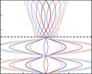
Figure 4. Dynamics with parametric variation. Non-dimensional velocity profiles in $y$ for parametric changes in $Re = \{0.1, 0.5, 1, 2, 10\} \times {Er} = \{0.1, 1, 10\}$, with $\nu = 0.1$, $\rho = 1$. The system response is shown only for the upper half-plane, where we also mark the length scales $\delta _f, \delta _s, \lambda$. The black dashed lines indicate the solid–fluid interface. Colours represent $t / T$, with the same colour bar as in figure 2.

4.5. Solid phase resonance

We conclude this section by investigating the conditions under which resonant solid deformations may occur. These might serve well applications such as elastometry, where high-amplitude peaks can provide unique footprints to characterize materials.

We begin by defining the gain function $|G| \geqslant 0$ as the ratio of solid to wall amplitude which, from (3.3), is given by the closed-form expression

(4.1)\begin{equation} |G| = \left\lvert \frac{{\rm i} \omega C}{\hat{V}_{{wall}}} \right\rvert = \frac{2}{\lvert ({\rm e}^{k_f-k_s} - {\rm e}^{-(k_f-k_s)}) ( 1 - \alpha ) - ({\rm e}^{k_f + k_s} - {\rm e}^{-(k_f + k_s)}) ( 1 + \alpha ) \rvert}, \end{equation}

where $k_f$ and $k_s$ are the fluid and solid wave contributions (see (3.4a,b)), and $\alpha = ({L_f}/{L_s}) ({k_s}/{k_f}) ( \rho \nu - \textrm {i}({\dot {\gamma }}/{ {Er}}))$ captures the degree of fluid–solid coupling.

In the limit case of a purely elastic solid ($\nu = 0$), the denominator of $G$ is always $> 0$, due to the non-zero contributions from the fluid phase ($k_f \neq 0$). The immediate implication is that unbounded resonance, $|G| \to \infty$, is not possible in our set-up because the fluid always dampens out high amplitudes in the solid phase. Thus interstitial fluids, besides providing lubrication as in synovial joints, may also prevent excessive deformations and subsequent failure of the soft, articular cartilage.

In figure 5(a), we plot $|G|$ as a function of $ {Er}, Re$ with $\nu = 0$. As can be seen, characteristic gain peaks ($|G| > 1$, bright yellow) take place and manifest as families of hyperbolae $Re \, {Er} = k^2$. Here, $k = {{\rm \pi} }/{\lambda }$ corresponds to discrete harmonic wavenumbers with wavelength $\lambda = ( {\rm \pi}^2\,Re\, {Er} )^{-{1}/{2}}$, from table 1. Hence higher $k$ corresponds to higher harmonics. To gain further intuition, we fix $Re = 1$ (chosen because of its dynamic richness, see figure 4), and plot $|G|$ versus $ {Er}$ to obtain the red curve of figure 5(c). We see four distinct high-gain peaks $\unicode{x24EA}$ – $\unicode{x2462}$ of increasing amplitude, where the numbers represent the standing wave mode. In the cases $\unicode{x2460}$ – $\unicode{x2462}$, the solid displaces more than the driving wall (figures 5d–f), with velocity profiles corresponding to the first three harmonics. Case $\unicode{x24EA}$ is characterized by the fact that maximal amplitudes occur at the interface, and not in the bulk, thus behaving as a standing wave with a free end at the interface.

Figure 5. High amplitude gains. Phase map of $|G|$ as a function of $Re, {Er}$ shows distinct regions of high (bright yellow) and low (dark blue) gains in cases with viscosity ratios (a) $\nu = 0$, (b) $\nu = 10^{-2}$, with maxima in both cases along $Re\, {Er} = k^2$ (white dashed line), where $k$ increases in the direction of the arrow in (a). We fix $Re = 1$ and plot $|G|$ against $ {Er}$ along the black dashed line in (a) for different viscosity ratios $\nu$ (coloured) in (c), which shows four distinct peaks, $\unicode{x24EA}$ to $\unicode{x2462}$, at $ {Er} = 0.14, 1.3, 4.27, 9.27$. Increasing viscosity decreases $|G|$ peaks, especially for $\unicode{x2461}$ and $\unicode{x2462}$. Plotting the velocity profiles corresponding to $\unicode{x2460}$ to $\unicode{x2462}$ at $\nu = 0$ in (d–f) and $\nu = 10^{-2}$ in (g–i) reveals that they resemble harmonic standing waves within the solid. We confirm that these high-gain results are indeed physical by plotting equivalent 2-D DNS results as black scatter points in (d,g) where we notice agreement between the curves.

Realistic materials include internal dissipation effects, which we enable here by adding viscosity to the solid. This reduces $|G|$ amplitudes, but preserves the hyperbolic structure of peaks, as seen in figure 5(b).

Finally, 2-D DNS simulations for $\nu = 0, 10^{-2}$ (black scatter points in figures 5d,g) validate our model predictions. Since it is challenging numerically to capture these high-gain regimes, we propose $Re = 1$, $ {Er} = 1.3$, $\nu = {0, 10^{-2}}$ for benchmarking numerical simulations, in addition to the parameter sets presented in § 4.4.

We have thus provided analytical solutions for the dynamics of a visco-elastic linear Kelvin–Voigt solid immersed in an oscillatory Couette flow system. We have derived a general solution to account for arbitrary solid densities and viscosities in our set-up, using two approaches – one in modal space generalizing the previous work of Sugiyama et al. (Reference Sugiyama, Ii, Takeuchi, Takagi and Matsumoto2011), and one in physical space. As a special limiting case, we recover the original solution of Sugiyama et al. (Reference Sugiyama, Ii, Takeuchi, Takagi and Matsumoto2011) for a density-matched solid with zero viscosity. Additionally, we recover analytical solutions of single-fluid (Landau & Lifshitz Reference Landau and Lifshitz1987) and multi-fluid (Sim Reference Sim2006; Leclaire et al. Reference Leclaire, Pellerin, Reggio and Trépanier2014) Stokes–Couette flows in the limit of zero solid elastic shear modulus. Further, our solutions compare well against DNS results (figure 3). They are found to exhibit a range of behaviours (figure 4), including high gains (figure 5), with potential applications in biophysics and engineering. Next, we discuss the case of a nonlinear Kelvin–Voigt solid, which presents higher-order nonlinear effects within the solid.

5.1. Modal solutions

In the case of a nonlinear Kelvin–Voigt solid, characterized by $c_{3} \neq 0$, the elastic stress is proportional to the cubic power of strain (see (2.7)), which signifies a higher-order nonlinear response to deformations. The resulting equations, whose nonlinearity is captured overall via the parameter $c = {c_{3}} / {c_{1}}$, resist closed-form analytical solutions. Then, to investigate the system response in this setting, we derive a solution using the Fourier series machinery of § 3.2, which we then evaluate numerically.

The solution strategy here is to employ a Fourier pseudo-spectral collocation scheme (Sugiyama et al. Reference Sugiyama, Ii, Takeuchi, Takagi and Matsumoto2011) for evaluating the nonlinear stress terms $\sigma _{{NL}, k}$ in the governing equation (3.10), at a finite set of grid points $x_j = (j + \frac {1}{2})\, {\rm \Delta} x$, with ${\rm \Delta} x= {L_s}/{K}$. All other terms are treated as described in § 3.2.

Armed with this spatial discretization, we employ a numerical time integration scheme to evolve the nonlinear equations (3.9) and (3.10). We use a second-order constant timestepper (of timestep ${\rm \Delta} t$) comprised of mixed Crank–Nicolson (implicit, for stability in the viscous updates) and explicit Nyström (midpoint) rule for the second-order time derivatives (Hairer, Nørsett & Wanner Reference Hairer, Nørsett and Wanner1991). If we denote the $n$th time level $t = n\, {\rm \Delta} t$ by a superscript $n$, then the prescribed wall velocity takes the analytical form

(5.1)\begin{equation} V_{{wall}}^{(n+1)} := V_{{wall}}((n+1)\,{\rm \Delta} t) = {\rm Im} [ \hat{V}_{{wall}} \exp ({\rm i} \omega ((n+1)\,{\rm \Delta} t)) ]. \end{equation}

For the interface displacement $U_{I}$ and fluid velocity update in (3.9), we use the Crank–Nicolson scheme (Hairer et al. Reference Hairer, Nørsett and Wanner1991)

(5.2)\begin{equation} U_{I}^{(n+1)} \approx U_{I}^{(n)}+\frac{{\rm \Delta} t}{2}\, (V_{I}^{(n+1)}+V_{I}^{(n)}) + {O} ( {\rm \Delta} t^2 ), \end{equation}

and for updating the interface velocity $V_{I}$ and solid displacements in (3.10), we utilize the explicit Nyström (midpoint) rule

(5.3)\begin{equation} \left( \frac{\mathrm{d} V_{I}}{\mathrm{d} t} \right)^{(n)} \approx \frac{ V_{I}^{(n+1)} - V_{I}^{(n-1)} }{2\,{\rm \Delta} t} + {O} ( {\rm \Delta} t^2 ). \end{equation}

Upon substituting these discretizations in the governing equations (3.9) and 3.10, and by invoking the modal stress balance of (3.11) at every step, we obtain the solution, after standard (but tedious) algebraic manipulations. For brevity, we omit derivation details, which can be found in supplementary material § 9.

5.2. Analysis of system behaviour

We first validate our solutions against DNS (figure 6) in the set-up of figure 3, but with $c = 4$ instead of $c=0$. The choice of $c$ is consistent with established biological tissue models (Raghavan & Vorp Reference Raghavan and Vorp2000). As can be seen in figure 6(a), the solid velocity profiles exhibit characteristic high-curvature bends (marked), differently from the linear Kelvin–Voigt case (figure 3) on account of the additional material nonlinearity. Further, as illustrated in figure 6(c), our solutions are found to agree well with DNS.

Figure 6. Comparison against simulations. (a) Non-dimensional velocity profiles in $y$, for a nonlinear Kelvin–Voigt solid. The system response is shown only in the upper half-plane. This system is characterized by $Re = 2$, $ {Er} = 1$, $\nu = 0.1$, $c = c_{3} / c_{1} = 4$, $\delta _f = 0.4$, $\delta _s = 0.126$, $\lambda = 0.225$. Additional details can be found in supplementary material § 6. Colours indicate $t / T$. We also mark a high curvature bend in the profile with a black arrow. (b) We solve the above problem through 2-D DNS (Bhosale et al. Reference Bhosale, Parthasarathy and Gazzola2021) with corresponding simulation parameters reported in supplementary material § 6. In this image, we mark the $x$-velocity field (orange/blue represent positive/negative velocity) and deformation contours within the solid, with the interface marked (black, thick solid) for visual clarity. Upon plotting the velocity profiles at the highlighted station (black, dashed) in the centre of the domain, we see good agreement with our results across all times as shown in (c). For the sake of clarity, we show profiles at only two different time instances. Here, numerical results are plotted with scatter points, whereas present results are plotted with a solid line.

Next, in the spirit of figure 4, we highlight system responses upon varying both degree of solid nonlinearity ($c$) and viscosity ($Re$). Throughout this exploration, we fix the elastic to viscous contributions by setting $Er = 1$ and $\nu = 0.1$. These values are informed by the rich dynamics of figures 4(b,e,h,k,n). We then choose values that span $(c, Re) \in \{1, 5, 10\} \times \{0.1, 0.5, 1, 2, 10\}$, and report the responses of the system in figure 7.

Figure 7. Dynamics with parametric variation. Non-dimensional velocity profile in $y$ for parametric changes that span $(c, Re) \in \{1, 5, 10\} \times \{0.1, 0.5, 1, 2, 10\}$ with $ {Er} = 1$, $\nu = 0.1$, $\rho = 1$. The system response is shown only in the upper half-plane. The black dashed lines indicate the solid–fluid interface. Colours represent $t / T$, with the same colour bar as in figure 2. We also mark the location of prominent high-curvature bends in the profiles with a black arrow.

For solids with small $c$, we expect dynamics similar to the linear Kelvin–Voigt counterpart. This is confirmed from the solid zone profiles in figures 7(a,d,g,j,m). Increasing the nonlinearity coefficient stiffens the solid, constraining deformation velocities (narrower envelopes) as well as producing sharper bends (marked), as we move from left to right in figure 7.

Changing viscosity ($Re$) affects the response in a fashion similar to the linear case (figure 4), where profile curvatures in both fluid and solid phases get concentrated progressively within sharper boundary layers, as we move from top to bottom in figure 7.

Finally, we investigate whether the high-gain regimes seen in § 4.5 exist for nonlinear Kelvin–Voigt solids, and if so, under what conditions. Here, unlike § 4.5, there is no mathematical guidance to identify high-gain parameters, thus we explore the $ {Er}$–$Re$ phase space numerically for the representative cases $c = 1$ (figure 8a) and $c = 5$ (figure 8b). For $c =1$, we see in figure 8(a) that high-gain peaks (bright yellow) still occur in a regular structure, although they are less pronounced and depart from the hyperbolae seen in the linear Kelvin–Voigt case, now lying on the curve-fit $Re\, {Er}^{0.5} = \textit {const}$. In figure 8(c), we report the velocity profiles of a representative high-gain case, and note that $|v / \hat {V}_{{wall}}|$ hardly exceeds 1, as opposed to the linear Kelvin–Voigt cases of figure 5. As we increase $c$ from $1$ to $5$, we observe that the peaks spread apart and lie on the curve-fit $Re\, {Er}^{0.4} = \textrm {const.}$, and gains diminish further (figure 8b). We conclude that the cubic term that characterizes nonlinear Kelvin–Voigt solids stiffens the material locally, reducing its propensity to deform and shear.

Figure 8. High amplitude gains for a nonlinear Kelvin–Voigt solid. Phase map of numerically measured $|G|$ as a function of $Re, {Er}$, for $\nu = 10^{-3}$ and (a) $c = 1$, (b) $c = 5$, shows regions of high (bright yellow) and low (dark blue) gains with maxima along $Re\, {Er}^{0.5} = \textrm {const.}$ and $Re\, {Er}^{0.4} = \textrm {const.}$, respectively, deviating from the hyperbolae seen in the linear Kelvin–Voigt case. The curves are obtained from a numerical fitting procedure, with details reported in supplementary material § 10. Velocity profiles of a representative case with $Re = 0.2$, $ {Er} = 6$, $c = 1$ marked in (a) and plotted in (c) showcase high-gain bends (marked) characteristic of strong nonlinear effects in the solid.