2.1 Geometric constraints

In two dimensions, as the liquid surface is in equilibrium, the menisci at the two sides of the cylinder can be expressed as (Bhatnagar & Finn Reference Bhatnagar and Finn2016)

(2.1) $$\begin{eqnarray}{\displaystyle \frac{\unicode[STIX]{x1D705}u^{2}}{2}}+\cos \unicode[STIX]{x1D713}=1,\quad \unicode[STIX]{x1D713}\in [-\unicode[STIX]{x03C0},\unicode[STIX]{x03C0}],\end{eqnarray}$$

where $u$ is the height of the meniscus, $\unicode[STIX]{x1D713}$ is the inclination angle of the meniscus and $\unicode[STIX]{x1D705}=\unicode[STIX]{x1D70C}g/\unicode[STIX]{x1D70E}$ is the capillary constant, with the density difference $\unicode[STIX]{x1D70C}$ (positive) between gas and liquid, the gravitational acceleration $g$ and the surface tension $\unicode[STIX]{x1D70E}$ of the interface. Equation (2.1) can be obtained by integrating the parametric form of the Young–Laplace equation in two dimensions (which gives a conserved quantity $C=\unicode[STIX]{x1D705}u^{2}/2+\cos \unicode[STIX]{x1D713}$ ) and then determining $C=1$ from the condition at infinity (Princen Reference Princen and Matijević1969; Finn Reference Finn2010; Aspley et al. Reference Aspley, He and McCuan2015). Since the sign of the height $u$ is the same as that of the inclination angle $\unicode[STIX]{x1D713}$ , the expression of the height $u$ can be given by transforming (2.1)

(2.2) $$\begin{eqnarray}u={\displaystyle \frac{2}{\sqrt{\unicode[STIX]{x1D705}}}}\sin {\displaystyle \frac{\unicode[STIX]{x1D713}}{2}}.\end{eqnarray}$$

To omit unnecessary details, only the left side of the cylinder is considered, as shown in figure 1(c). The origin is arbitrary on the water line because the system has translation invariance along the $x$ direction. According to Young’s relation, the geometric relation between the cylinder surface and the meniscus is given by

(2.3) $$\begin{eqnarray}\unicode[STIX]{x1D719}_{l}=\unicode[STIX]{x1D711}_{l}+\unicode[STIX]{x1D703},\end{eqnarray}$$

where the angles $\unicode[STIX]{x1D719}_{l}=\unicode[STIX]{x03C0}/2-\unicode[STIX]{x1D713}_{l}$ and $\unicode[STIX]{x1D711}_{l}$ are measured clockwise, with reference to figure 1(c), starting from the horizontal line, to the unit normal vectors $\boldsymbol{n}_{m}$ and $\boldsymbol{n}_{s}$ , of the meniscus and the cylinder surface at the left contact point, respectively. The cylinder surface is expressed by the parametric function $\boldsymbol{r}(t)=[x(t),y(t)]$ , where the parametric expression is the same as that in Kemp & Siegel (Reference Kemp and Siegel2011). Meanwhile, the position and orientation of the cylinder are determined by $\boldsymbol{r}(t)$ . It is assumed that the parametrization is oriented counterclockwise and the derivative $\boldsymbol{r}^{\prime }(t)$ is never 0. The position vector of the left contact point is denoted by $\boldsymbol{r}(t_{l})$ . According to the geometric relation at the left contact point, the parameter $t_{l}$ and the angles $\unicode[STIX]{x1D711}_{l}$ and $\unicode[STIX]{x1D713}_{l}$ are related by

(2.4a,b ) $$\begin{eqnarray}x^{\prime }(t_{l})=\tan \unicode[STIX]{x1D711}_{l}y^{\prime }(t_{l})\quad \text{and}\quad y(t_{l})=u_{l},\end{eqnarray}$$

where the primes refer to derivatives $\text{d}/\text{d}t$ with respect to the parameter  $t$ . Since the cross-section is convex, equations (2.2)–(2.4) have a unique solution $\boldsymbol{r}(t_{l})$ for a specific contact angle $\unicode[STIX]{x1D703}$ and a specific geometry $\boldsymbol{r}(t)$ (see appendix A).

For the case of the right side, the equations used to determine $\boldsymbol{r}(t_{r})$ can be obtained by simply replacing the subscript $l$ with the subscript $r$ in (2.2)–(2.4), and modifying (2.4a ) to

(2.5) $$\begin{eqnarray}x^{\prime }(t_{r})=-\text{tan}\unicode[STIX]{x1D711}_{r}y^{\prime }(t_{r}).\end{eqnarray}$$

The angles $\unicode[STIX]{x1D719}_{r}$ and $\unicode[STIX]{x1D711}_{r}$ are measured counterclockwise. The subscript $l$ means that the quantities are measured at the left contact point while the subscript $r$ corresponds to the right contact point.

When the contact angle $\unicode[STIX]{x1D703}$ and the shape of the cross-section are given, the position vectors $\boldsymbol{r}(t_{l})$ and $\boldsymbol{r}(t_{r})$ and the corresponding angles $\unicode[STIX]{x1D711}$ are uniquely determined by the position and orientation of the cylinder. The six quantities $x_{l}$ , $x_{r}$ , $u_{l}$ , $u_{r}$ , $\unicode[STIX]{x1D711}_{l}$ and $\unicode[STIX]{x1D711}_{r}$ are called basic geometric quantities in the model, because they can be uniquely determined by the geometric constraints.

2.2 Forces

When the contact points are obtained from the position and orientation of the cylinder, the configuration is determined. The resultant force $\boldsymbol{f}_{net}$ acting on the cylinder can be given by

(2.6) $$\begin{eqnarray}\boldsymbol{f}_{net}=\boldsymbol{f}_{t}^{l}+\boldsymbol{f}_{t}^{r}+\boldsymbol{f}_{p}+\boldsymbol{B}+\boldsymbol{G}.\end{eqnarray}$$

The surface tension forces $\boldsymbol{f}_{t}^{l}$ and $\boldsymbol{f}_{t}^{r}$ at the left and right contact points are

(2.7a,b ) $$\begin{eqnarray}\boldsymbol{f}_{t}^{l}=-\unicode[STIX]{x1D70E}(\sin \unicode[STIX]{x1D719}_{l}\boldsymbol{e}_{i}+\cos \unicode[STIX]{x1D719}_{l}\boldsymbol{e}_{j})\quad \text{and}\quad \boldsymbol{f}_{t}^{r}=\unicode[STIX]{x1D70E}(\sin \unicode[STIX]{x1D719}_{r}\boldsymbol{e}_{i}-\cos \unicode[STIX]{x1D719}_{r}\boldsymbol{e}_{j}),\end{eqnarray}$$

respectively. The force $\boldsymbol{P}$ due to the pressure $p$ can be given by the integral over the wetted cylinder surface $S_{w}$ :

(2.8) $$\begin{eqnarray}\boldsymbol{P}=\int _{S_{w}}-p\boldsymbol{n}_{s}\,\text{d}s=\int _{S_{w}}\unicode[STIX]{x1D70C}gy\boldsymbol{n}_{s}\,\text{d}s.\end{eqnarray}$$

However, the expression (2.8) is inconvenient to actually apply to calculation. By applying Green’s theorem to (2.8), the force $\boldsymbol{P}$ can be rewritten as

(2.9) $$\begin{eqnarray}\int _{S_{w}}\unicode[STIX]{x1D70C}gy\boldsymbol{n}_{s}\,\text{d}s=\unicode[STIX]{x1D70C}gV_{B}\boldsymbol{e}_{j}+\int _{L_{c}}p_{c}\boldsymbol{n}_{c}\,\text{d}l,\end{eqnarray}$$

where $V_{B}$ denotes the area of the shaded section in figure 1(b) (i.e. the section submerged in the liquid), and $p_{c}=\unicode[STIX]{x1D70C}gy$ is the compensating pressure on the straight line $L_{c}$ between the contact points with the unit normal vectors $\boldsymbol{n}_{c}$ of $L_{c}$ directed inward toward the shaded section. Equation (2.9) expresses the decomposition of the force $\boldsymbol{P}$ into the compensating pressure force $\boldsymbol{f}_{p}$ and the buoyancy force $\boldsymbol{B}$ , while there is another decomposition of $\boldsymbol{P}$ adopted in, e.g. Keller (Reference Keller1998). Keller (Reference Keller1998) calculated the pressure force $\boldsymbol{P}$ by directly integrating $p$ over the wetted cylinder surface. Results shown that the vertical component of $\boldsymbol{P}$ is equal to the weight of the liquid that occupies the volume whose boundaries comprise the undisturbed interface, the vertical lines between the contact points and the undisturbed interface and the wetted surface of the cylinder (Keller Reference Keller1998). The two methods of decomposition are equivalent from the point of view of force. The force $\boldsymbol{f}_{p}$ can be obtained by integrating $p_{c}\boldsymbol{n}_{c}$ on the line, given by

(2.10) $$\begin{eqnarray}\boldsymbol{f}_{p}={\displaystyle \frac{\unicode[STIX]{x1D70C}g}{2}}[(u_{r}^{2}-u_{l}^{2})\boldsymbol{e}_{i}-(x_{r}-x_{l})(u_{l}+u_{r})\boldsymbol{e}_{j}],\end{eqnarray}$$

where the first vector on the right-hand side of (2.10) is equal to the horizontal component of the pressure force provided by Keller (Reference Keller1998).

The horizontal resultant force on the cylinder is the sum of the horizontal components of the forces $\boldsymbol{f}_{p}$ , $\boldsymbol{f}_{t}^{l}$ and $\boldsymbol{f}_{t}^{r}$ :

(2.11) $$\begin{eqnarray}f_{net}^{h}=\unicode[STIX]{x1D70E}\left[{\displaystyle \frac{\unicode[STIX]{x1D705}}{2}}(u_{r}^{2}-u_{l}^{2})+(\sin \unicode[STIX]{x1D719}_{r}-\sin \unicode[STIX]{x1D719}_{l})\right].\end{eqnarray}$$

Using (2.1), it is found that the horizontal force $f_{net}^{h}$ is always zero, which means that the horizontal equilibrium condition is automatically satisfied. The horizontal resultant force induced by the surface tension imbalance has been investigated by Janssens, Chaurasia & Fried (Reference Janssens, Chaurasia and Fried2017). From (2.6), (2.7) and (2.10), the vertical resultant force,

(2.12) $$\begin{eqnarray}f_{net}^{v}=-{\displaystyle \frac{\unicode[STIX]{x1D70C}g}{2}}(x_{r}-x_{l})(u_{l}+u_{r})-\unicode[STIX]{x1D70E}(\cos \unicode[STIX]{x1D719}_{r}+\cos \unicode[STIX]{x1D719}_{l})+\unicode[STIX]{x1D70C}gV_{B}-mg,\end{eqnarray}$$

can be calculated with the position vectors of the contact points $\boldsymbol{r}(t_{l})=(x_{l},u_{l})$ and $\boldsymbol{r}(t_{r})=(x_{r},u_{r})$ , and the angles $\unicode[STIX]{x1D719}_{l}$ and $\unicode[STIX]{x1D719}_{r}$ , where $m$ is the mass of the cylinder. As discussed in the previous section, the basic geometric quantities depend only on the position and orientation of the cylinder. Thus, when the contact angle and the shape of the cross-section are given, the resultant force can be calculated from the position and orientation of the cylinder.

2.3 Vertical equilibrium and stability

After determining the relation between the resultant force and the position and orientation of the cylinder, the next step is to find the equilibrium position. However, it is inconvenient to calculate the equilibrium position by solving $f_{net}^{v}=0$ directly, because the expression for $V_{B}$ in (2.12) is difficult to determine without a given cross-section. An alternative is to calculate the force variation $\unicode[STIX]{x1D6FF}f_{net}^{v}$ corresponding to an infinitesimal displacement $\unicode[STIX]{x1D6FF}h$ in height of the cylinder with a fixed orientation and a given height $h^{\ast }$ (see figure 2 a), and then to use the function $\unicode[STIX]{x1D6FF}f_{net}^{v}/\unicode[STIX]{x1D6FF}h$ and the force $f_{net}^{v}$ given by (2.12) as the ordinary differential equation and the initial condition, respectively, to form an initial value problem (IVP):

(2.13) $$\begin{eqnarray}\left.\begin{array}{@{}c@{}}{\dot{f}}=\unicode[STIX]{x1D6FF}f_{net}^{v}/\unicode[STIX]{x1D6FF}h,\\ f(h^{\ast })=f_{net}^{v},\end{array}\right\}\end{eqnarray}$$

where $h$ denotes the height of the cylinder measured from the undisturbed liquid surface and a dot over a character denotes the derivative of the corresponding displacement. It is noted that all the variations in the model are considered in the context of the principle of virtual work dating back to Bernoulli. The reference point $p_{h}$ for determining the height $h$ can be any point, e.g. the centroid of the cross-section. This problem has a unique solution, which means that the vertical force $f_{net}^{v}$ is entirely determined by the height $h$ . The vertical equilibria can be obtained from the force profile, and their stabilities can be determined by the derivatives ${\dot{f}}$ , where ${\dot{f}}<0$ and ${\dot{f}}>0$ correspond to stable and unstable equilibria, respectively.

Figure 2. An infinitesimal displacement in $h$ results in the displacement of the contact points: (a)  $\unicode[STIX]{x1D6FF}\boldsymbol{r}_{l}$ and $\unicode[STIX]{x1D6FF}\boldsymbol{r}_{r}$ for the reference frame fixed in the liquid, and (b) $\unicode[STIX]{x1D6FF}\bar{\boldsymbol{r}}_{l}$ and $\unicode[STIX]{x1D6FF}\bar{\boldsymbol{r}}_{r}$ for the reference frame fixed in the solid. The point $p_{h}$ is the reference point for the height $h$ . The horizontal thick dot-dash line and the horizontal thin dot-dash line are the water lines before and after the displacement of the cylinder, respectively. The blue thick and red thin dashed lines are the lines $L_{c}$ before and after the displacement of the cylinder, respectively.

Because the weight force $\boldsymbol{G}$ is constant, the variation of the net force $f_{net}^{v}$ is deduced from (2.12) as

(2.14) $$\begin{eqnarray}\displaystyle \unicode[STIX]{x1D6FF}f_{net}^{v} & = & \displaystyle -{\displaystyle \frac{\unicode[STIX]{x1D70C}g}{2}}[(u_{l}+u_{r})(\unicode[STIX]{x1D6FF}x_{r}-\unicode[STIX]{x1D6FF}x_{l})+(x_{r}-x_{l})(\unicode[STIX]{x1D6FF}u_{l}+\unicode[STIX]{x1D6FF}u_{r})]\nonumber\\ \displaystyle & & \displaystyle +\,\unicode[STIX]{x1D70E}(\sin \unicode[STIX]{x1D719}_{l}\unicode[STIX]{x1D6FF}\unicode[STIX]{x1D711}_{l}+\sin \unicode[STIX]{x1D719}_{r}\unicode[STIX]{x1D6FF}\unicode[STIX]{x1D711}_{r})+\unicode[STIX]{x1D70C}g\unicode[STIX]{x1D6FF}V_{B}.\end{eqnarray}$$

The variations $(\unicode[STIX]{x1D6FF}x_{l},\unicode[STIX]{x1D6FF}u_{l})$ , $\unicode[STIX]{x1D6FF}\unicode[STIX]{x1D711}_{l}$ and $\unicode[STIX]{x1D6FF}V_{B}$ to the first order in $\unicode[STIX]{x1D6FF}h$ are shown as

(2.15a ) $$\begin{eqnarray}\displaystyle & \displaystyle \unicode[STIX]{x1D6FF}x_{l}=-{\displaystyle \frac{\sqrt{\unicode[STIX]{x1D705}}R_{l}\sin \unicode[STIX]{x1D711}_{l}}{\sqrt{\unicode[STIX]{x1D705}}R_{l}\cos \unicode[STIX]{x1D711}_{l}+\sin \left({\displaystyle \frac{\unicode[STIX]{x1D711}_{l}+\unicode[STIX]{x1D703}}{2}}+{\displaystyle \frac{\unicode[STIX]{x03C0}}{4}}\right)}}\unicode[STIX]{x1D6FF}h, & \displaystyle\end{eqnarray}$$

(2.15b ) $$\begin{eqnarray}\displaystyle & \displaystyle \unicode[STIX]{x1D6FF}u_{l}={\displaystyle \frac{\sin \left({\displaystyle \frac{\unicode[STIX]{x1D711}_{l}+\unicode[STIX]{x1D703}}{2}}+{\displaystyle \frac{\unicode[STIX]{x03C0}}{4}}\right)}{\sqrt{\unicode[STIX]{x1D705}}R_{l}\cos \unicode[STIX]{x1D711}_{l}+\sin \left({\displaystyle \frac{\unicode[STIX]{x1D711}_{l}+\unicode[STIX]{x1D703}}{2}}+{\displaystyle \frac{\unicode[STIX]{x03C0}}{4}}\right)}}\unicode[STIX]{x1D6FF}h, & \displaystyle\end{eqnarray}$$

(2.15c ) $$\begin{eqnarray}\displaystyle & \displaystyle \unicode[STIX]{x1D6FF}\unicode[STIX]{x1D711}_{l}=-{\displaystyle \frac{\sqrt{\unicode[STIX]{x1D705}}}{\sqrt{\unicode[STIX]{x1D705}}R_{l}\cos \unicode[STIX]{x1D711}_{l}+\sin \left({\displaystyle \frac{\unicode[STIX]{x1D711}_{l}+\unicode[STIX]{x1D703}}{2}}+{\displaystyle \frac{\unicode[STIX]{x03C0}}{4}}\right)}}\unicode[STIX]{x1D6FF}h, & \displaystyle\end{eqnarray}$$

(2.15d ) $$\begin{eqnarray}\displaystyle & \displaystyle \unicode[STIX]{x1D6FF}V_{B}={\textstyle \frac{1}{2}}[(u_{l}-u_{r})(\unicode[STIX]{x1D6FF}x_{r}+\unicode[STIX]{x1D6FF}x_{l})+(x_{r}-x_{l})(\unicode[STIX]{x1D6FF}u_{l}+\unicode[STIX]{x1D6FF}u_{r}-2\unicode[STIX]{x1D6FF}h)], & \displaystyle\end{eqnarray}$$

$R_{l}$

$\unicode[STIX]{x1D6FF}h$

$\unicode[STIX]{x1D6FF}h$

$(\unicode[STIX]{x1D6FF}x_{r},\unicode[STIX]{x1D6FF}u_{r})$

$\unicode[STIX]{x1D6FF}\unicode[STIX]{x1D711}_{r}$

$l$

$r$

(2.16) $$\begin{eqnarray}\unicode[STIX]{x1D6FF}x_{r}={\displaystyle \frac{\sqrt{\unicode[STIX]{x1D705}}R_{r}\sin \unicode[STIX]{x1D711}_{r}}{\sqrt{\unicode[STIX]{x1D705}}R_{r}\cos \unicode[STIX]{x1D711}_{r}+\sin \left({\displaystyle \frac{\unicode[STIX]{x1D711}_{r}+\unicode[STIX]{x1D703}}{2}}+{\displaystyle \frac{\unicode[STIX]{x03C0}}{4}}\right)}}\unicode[STIX]{x1D6FF}h.\end{eqnarray}$$

Thus, the differential equation ${\dot{f}}$ in (2.13) is related to the eight quantities at the contact points: $x_{l}$ , $x_{r}$ , $u_{l}$ , $u_{r}$ , $\unicode[STIX]{x1D711}_{l}$ , $\unicode[STIX]{x1D711}_{r}$ , $R_{l}$ and $R_{r}$ . Accordingly, an IVP in six dimensions is formed to calculate the basic geometric quantities. The radii of curvature $R_{l}$ and $R_{r}$ can be determined by the basic geometric quantities and the height $h$ . The IVP for the basic geometric quantities consists of the system of equations: six ODEs and the corresponding initial conditions. For instance, the ODE for $x_{l}$ is ${\dot{x}}_{l}=\unicode[STIX]{x1D6FF}x_{l}/\unicode[STIX]{x1D6FF}h$ together with the initial condition $x_{l}(h^{\ast })=x_{l}^{\ast }$ . By solving the above IVP, the values of the quantities in (2.13) are obtained. Therefore the resultant force profile can be obtained by solving the system of ODEs together with the initial conditions:

(2.17) $$\begin{eqnarray}\left.\begin{array}{@{}c@{}}{\dot{f}}=\unicode[STIX]{x1D6FF}f_{net}^{v}/\unicode[STIX]{x1D6FF}h,{\dot{x}}_{l}=\unicode[STIX]{x1D6FF}x_{l}/\unicode[STIX]{x1D6FF}h,\ldots ,\dot{\unicode[STIX]{x1D711}}_{r}=\unicode[STIX]{x1D6FF}\unicode[STIX]{x1D711}_{r}/\unicode[STIX]{x1D6FF}h,\\ f(h^{\ast })=f_{net}^{v},x_{l}(h^{\ast })=x_{l}^{\ast },\ldots ,\unicode[STIX]{x1D711}_{r}(h^{\ast })=\unicode[STIX]{x1D711}_{r}^{\ast },\end{array}\right\}\end{eqnarray}$$

where the omissions are the ODEs for the basic geometric quantities not shown and the corresponding initial conditions. A detailed description on the derivations of (2.15a–d ) is provided in appendix B.

In order to validate the model, the force profile of a uniform cylinder floating in an unbounded bath is obtained by using our numerical code. For simplicity, the Euler method is adopted to solve (2.17). The force analysis of this configuration was given by Princen (Reference Princen and Matijević1969), who derived an equilibrium equation for a uniform cylinder floating on a liquid surface. Following Princen (Reference Princen and Matijević1969), Rapacchietta et al. (Reference Rapacchietta, Neumann and Omenyi1977) developed a non-equilibrium model and provided the analytical expression of the resultant forces exerted on a uniform cylinder. The numerical result in this paper is compared to the analytical expression presented by Rapacchietta et al. (Reference Rapacchietta, Neumann and Omenyi1977). The resultant force exerted on the uniform cylinder is given by

(2.18) $$\begin{eqnarray}\displaystyle f_{net}^{v} & = & \displaystyle -2\unicode[STIX]{x1D70E}\cos (\unicode[STIX]{x1D703}+\unicode[STIX]{x1D711}_{r})-mg\nonumber\\ \displaystyle & & \displaystyle +\,\unicode[STIX]{x1D70C}gr^{2}\left\{\unicode[STIX]{x1D711}_{r}+{\displaystyle \frac{\unicode[STIX]{x03C0}}{2}}-\cos \unicode[STIX]{x1D711}_{r}\left[{\displaystyle \frac{4}{\sqrt{\unicode[STIX]{x1D705}}r}}\cos \left({\displaystyle \frac{\unicode[STIX]{x1D703}+\unicode[STIX]{x1D711}_{r}}{2}}+{\displaystyle \frac{\unicode[STIX]{x03C0}}{4}}\right)-\sin \unicode[STIX]{x1D711}_{r}\right]\!\right\},\end{eqnarray}$$

where $r$ denotes the radius of the cylinder.

Figure 3(a) compares the numerical result to the analytical solution of Rapacchietta et al. (Reference Rapacchietta, Neumann and Omenyi1977) for a uniform cylinder. The inset shows the relative error of the numerical simulation. An excellent agreement is found, demonstrating the validity of our numerical code for the force profile of the cylinder. We assume that all configurations are in equilibrium, i.e. the mass of the cylinder is given as a function of the position of the cylinder to counteract the other forces. During the numerical simulation, the stability in the vertical direction can easily be obtained from the first derivative of the force, as shown in figure 3(b). A theoretical stability analysis for this case was conducted by Bhatnagar & Finn (Reference Bhatnagar and Finn2006), who solved an eigenvalue problem associated with the second variation of energy to predict the vertical stability of the cylinder. Following the approach of Bhatnagar & Finn (Reference Bhatnagar and Finn2006) with some modifications, Chen & Siegel (Reference Chen and Siegel2018) predicted the vertical stability by using the relation between the total energy and the resultant force.

In the mathematical model, the variation of the resultant force is described as a function of the basic geometric quantities and their variations, transforming a number of irrelevant and repetitive problems of solving the resultant force in one problem similar to the IVP. The advantages of this model are that it avoids repetition of § 2.1 for determining the configurations in which the menisci satisfy the Young–Laplace equation with Young’s relation, and transforms the change of the configuration to the variations of the basic geometric quantities: $\unicode[STIX]{x1D6FF}x_{l}$ , $\unicode[STIX]{x1D6FF}x_{r}$ , $\unicode[STIX]{x1D6FF}u_{l}$ , $\unicode[STIX]{x1D6FF}u_{r}$ , $\unicode[STIX]{x1D6FF}\unicode[STIX]{x1D711}_{l}$ and $\unicode[STIX]{x1D6FF}\unicode[STIX]{x1D711}_{r}$ . Thus, the complex configurations can be obtained by integrating a simple configuration. For instance, the cylinder floating in an infinite bath without gravity (see Kemp & Siegel (Reference Kemp and Siegel2011)) can be used as the initial configuration in the model. The simulations for other cases are shown in § 3.

Figure 3. (a) Comparison between the numerical result and the analytical solution in Rapacchietta et al. (Reference Rapacchietta, Neumann and Omenyi1977). The following values of parameters are used: $r=1.5~\text{mm}$ , $\unicode[STIX]{x1D703}=\unicode[STIX]{x03C0}/2$ , $\unicode[STIX]{x1D70E}=0.072~\text{N}~\text{m}^{-1}$ , $g=9.81~\text{m}~\text{s}^{-2}$ , $\unicode[STIX]{x1D70C}=1000~\text{kg}~\text{m}^{-3}$ , $m=\unicode[STIX]{x1D70C}\unicode[STIX]{x03C0}r^{2}/2$ and $\unicode[STIX]{x1D6FF}h=-\text{3.75}\times 10^{-7}~\text{m}$ . In the following calculations, the values of $\unicode[STIX]{x1D70C}$ , $g$ and $\unicode[STIX]{x1D70E}$ remain constant. The inset shows the relative error of the numerical simulation. (b) The first derivative of force indicates the stability of the cylinder, where A is a stable point, C is an unstable point and B is the turning point. The typical configurations are presented, where the red curves are menisci, the circles are cylinders and the dot-dash lines are water lines.

2.4 Rotational equilibrium and stability

When a vertical equilibrium is achieved, the forces with a resultant moment on the cylinder form a couple, which has the same moment $\boldsymbol{M}$ about all points. Thus, the reference point of the resultant moment can be any point. Selecting the origin 0 as the reference point, the moment can be given by

(2.19) $$\begin{eqnarray}\boldsymbol{M}=\boldsymbol{r}_{l}\times \boldsymbol{f}_{t}^{l}+\boldsymbol{r}_{r}\times \boldsymbol{f}_{t}^{r}+\boldsymbol{r}_{p}\times \boldsymbol{f}_{p}+\boldsymbol{r}_{B}\times \boldsymbol{B}+\boldsymbol{r}_{G}\times \boldsymbol{G},\end{eqnarray}$$

where $\boldsymbol{r}_{p}$ , $\boldsymbol{r}_{B}$ and $\boldsymbol{r}_{G}$ denote the position vectors of $\boldsymbol{f}_{p}$ , $\boldsymbol{B}$ and $\boldsymbol{G}$ , respectively. The position vector $\boldsymbol{r}_{p}$ depends on the two vectors $\boldsymbol{r}_{l}$ and $\boldsymbol{r}_{r}$ as:

(2.20) $$\begin{eqnarray}\boldsymbol{r}_{p}=\unicode[STIX]{x1D709}_{l}\boldsymbol{r}_{l}+\unicode[STIX]{x1D709}_{r}\boldsymbol{r}_{r},\end{eqnarray}$$

where

(2.21a,b ) $$\begin{eqnarray}\unicode[STIX]{x1D709}_{l}={\displaystyle \frac{2u_{l}+u_{r}}{3u_{l}+3u_{r}}}\quad \text{and}\quad \unicode[STIX]{x1D709}_{r}={\displaystyle \frac{u_{l}+2u_{r}}{3u_{l}+3u_{r}}}.\end{eqnarray}$$

We suppose that the shaded area $V_{B}$ , the mass $m$ and their centres $\boldsymbol{r}_{B}$ and $\boldsymbol{r}_{G}$ in figure 1(b) have been determined from the cross-section and the contact points $\boldsymbol{r}_{l}$ and $\boldsymbol{r}_{r}$ . The moment $\boldsymbol{M}$ can be calculated by (2.19).

Figure 4. An infinitesimal rotation $\unicode[STIX]{x1D6FF}\unicode[STIX]{x1D700}$ results in the displacement of the contact points: (a)  $\unicode[STIX]{x1D6FF}\boldsymbol{r}_{l}$ and $\unicode[STIX]{x1D6FF}\boldsymbol{r}_{r}$ for the reference frame fixed in the liquid, and (b) $\unicode[STIX]{x1D6FF}\bar{\boldsymbol{r}}_{l}$ and $\unicode[STIX]{x1D6FF}\bar{\boldsymbol{r}}_{r}$ for the reference frame fixed in the solid. The point $p_{ro}$ is the instantaneous centre of rotation. The inclined black thin dot-dash line in (b) is the water line after the rotation $\unicode[STIX]{x1D6FF}\unicode[STIX]{x1D700}$ . The blue thick and red thin dashed lines are the lines $L_{c}$ before and after the rotation of the cylinder, respectively.

To deal with the rotational equilibria, we will use an analogous approach to § 2.3 to obtain the moment profile $\boldsymbol{M}(\unicode[STIX]{x1D700})$ . By rotating the cylinder counterclockwise around the point $p_{ro}$ by an infinitesimally small angle $\unicode[STIX]{x1D6FF}\unicode[STIX]{x1D700}$ (see figure 4 a), the change in the moment can be divided into four parts:

(2.22) $$\begin{eqnarray}\unicode[STIX]{x1D6FF}\boldsymbol{M}=\unicode[STIX]{x1D6FF}\boldsymbol{M}_{t}+\unicode[STIX]{x1D6FF}\boldsymbol{M}_{p}+\unicode[STIX]{x1D6FF}\boldsymbol{M}_{B}+\unicode[STIX]{x1D6FF}\boldsymbol{M}_{G},\end{eqnarray}$$

where

(2.23a ) $$\begin{eqnarray}\displaystyle & \displaystyle \unicode[STIX]{x1D6FF}\boldsymbol{M}_{t}=\unicode[STIX]{x1D6FF}\boldsymbol{r}_{l}\times \boldsymbol{f}_{t}^{l}+\unicode[STIX]{x1D6FF}\boldsymbol{r}_{r}\times \boldsymbol{f}_{t}^{r}+\boldsymbol{r}_{l}\times \unicode[STIX]{x1D6FF}\boldsymbol{f}_{t}^{l}+\boldsymbol{r}_{r}\times \unicode[STIX]{x1D6FF}\boldsymbol{f}_{t}^{r}, & \displaystyle\end{eqnarray}$$

(2.23b ) $$\begin{eqnarray}\displaystyle & \displaystyle \unicode[STIX]{x1D6FF}\boldsymbol{M}_{p}=\unicode[STIX]{x1D6FF}(\boldsymbol{r}_{p}\times \boldsymbol{f}_{p}), & \displaystyle\end{eqnarray}$$

(2.23c ) $$\begin{eqnarray}\displaystyle & \displaystyle \unicode[STIX]{x1D6FF}\boldsymbol{M}_{B}=\unicode[STIX]{x1D6FF}\boldsymbol{r}_{B}\times \boldsymbol{B}+\boldsymbol{r}_{B}\times \unicode[STIX]{x1D6FF}\boldsymbol{B}, & \displaystyle\end{eqnarray}$$

(2.23d ) $$\begin{eqnarray}\displaystyle & \displaystyle \unicode[STIX]{x1D6FF}\boldsymbol{M}_{G}=\unicode[STIX]{x1D6FF}\boldsymbol{r}_{G}\times \boldsymbol{G}, & \displaystyle\end{eqnarray}$$

Utilizing the same method as in § 2.3, an IVP to calculate the resultant moment $\boldsymbol{M}$ is formed as follows:

(2.24) $$\begin{eqnarray}\left.\begin{array}{@{}c@{}}{\dot{M}}=\unicode[STIX]{x1D6FF}M/\unicode[STIX]{x1D6FF}\unicode[STIX]{x1D700},\\ M(0)=M_{in},\end{array}\right\}\end{eqnarray}$$

where $M$ is the scalar projection of $\boldsymbol{M}$ in the direction of the $z$ axis, and the subscript $in$ denotes the initial condition. For simplicity, the resultant moment refers to its vector projection $M$ , because the other scalar projections are zero. The rotational equilibria can be obtained from the moment profile, and their stabilities can be determined by the derivatives ${\dot{M}}$ , where ${\dot{M}}<0$ and ${\dot{M}}>0$ correspond to stable and unstable equilibria, respectively.

To keep the resultant moment $M$ about any reference point constant, the force variation $\unicode[STIX]{x1D6FF}f_{net}^{v}$ corresponding to the infinitesimal displacement $\unicode[STIX]{x1D6FF}\unicode[STIX]{x1D700}$ must be $o(\unicode[STIX]{x1D6FF}\unicode[STIX]{x1D700})$ during rotation. From (2.14), the variation $\unicode[STIX]{x1D6FF}f_{net}^{v}$ can be expressed in terms of the variations $\unicode[STIX]{x1D6FF}\boldsymbol{r}_{l}$ , $\unicode[STIX]{x1D6FF}\boldsymbol{r}_{r}$ , $\unicode[STIX]{x1D6FF}\unicode[STIX]{x1D711}_{l}$ , $\unicode[STIX]{x1D6FF}\unicode[STIX]{x1D711}_{r}$ and $\unicode[STIX]{x1D6FF}V_{B}$ , which are linearly related to the rotational displacement $\unicode[STIX]{x1D6FF}\unicode[STIX]{x1D700}$ :

(2.25a ) $$\begin{eqnarray}\displaystyle & \displaystyle \unicode[STIX]{x1D6FF}x_{l}=\left[{\displaystyle \frac{\sqrt{\unicode[STIX]{x1D705}}\cos \unicode[STIX]{x1D711}_{l}L_{l}+\sin \left({\displaystyle \frac{\unicode[STIX]{x1D711}_{l}+\unicode[STIX]{x1D703}}{2}}+{\displaystyle \frac{\unicode[STIX]{x03C0}}{4}}\right)}{\sqrt{\unicode[STIX]{x1D705}}\cos \unicode[STIX]{x1D711}_{l}R_{l}+\sin \left({\displaystyle \frac{\unicode[STIX]{x1D711}_{l}+\unicode[STIX]{x1D703}}{2}}+{\displaystyle \frac{\unicode[STIX]{x03C0}}{4}}\right)}}\sin \unicode[STIX]{x1D711}_{l}R_{l}-(u_{l}-u_{ro})\right]\unicode[STIX]{x1D6FF}\unicode[STIX]{x1D700}, & \displaystyle\end{eqnarray}$$

(2.25b ) $$\begin{eqnarray}\displaystyle & \displaystyle \unicode[STIX]{x1D6FF}u_{l}={\displaystyle \frac{\sin \left({\displaystyle \frac{\unicode[STIX]{x1D711}_{l}+\unicode[STIX]{x1D703}}{2}}+{\displaystyle \frac{\unicode[STIX]{x03C0}}{4}}\right)\cos \unicode[STIX]{x1D711}_{l}(R_{l}-L_{l})}{\sqrt{\unicode[STIX]{x1D705}}\cos \unicode[STIX]{x1D711}_{l}R_{l}+\sin \left({\displaystyle \frac{\unicode[STIX]{x1D711}_{l}+\unicode[STIX]{x1D703}}{2}}+{\displaystyle \frac{\unicode[STIX]{x03C0}}{4}}\right)}}\unicode[STIX]{x1D6FF}\unicode[STIX]{x1D700}, & \displaystyle\end{eqnarray}$$

(2.25c ) $$\begin{eqnarray}\displaystyle & \displaystyle \unicode[STIX]{x1D6FF}\unicode[STIX]{x1D711}_{l}=-{\displaystyle \frac{\sqrt{\unicode[STIX]{x1D705}}\cos \unicode[STIX]{x1D711}_{l}(R_{l}-L_{l})}{\sqrt{\unicode[STIX]{x1D705}}\cos \unicode[STIX]{x1D711}_{l}R_{l}+\sin \left({\displaystyle \frac{\unicode[STIX]{x1D711}_{l}+\unicode[STIX]{x1D703}}{2}}+{\displaystyle \frac{\unicode[STIX]{x03C0}}{4}}\right)}}\unicode[STIX]{x1D6FF}\unicode[STIX]{x1D700}, & \displaystyle\end{eqnarray}$$

(2.25d ) $$\begin{eqnarray}\displaystyle \unicode[STIX]{x1D6FF}V_{B} & = & \displaystyle {\textstyle \frac{1}{2}}[(u_{l}-u_{r})(\unicode[STIX]{x1D6FF}x_{r}+\unicode[STIX]{x1D6FF}x_{l})+(x_{r}-x_{l})(\unicode[STIX]{x1D6FF}u_{l}+\unicode[STIX]{x1D6FF}u_{r})]\nonumber\\ \displaystyle & & \displaystyle +\,{\textstyle \frac{1}{2}}[(u_{l}-u_{r})(u_{r}+u_{l}-2u_{ro})+(x_{l}-x_{r})(x_{l}+x_{r}-2x_{ro})]\unicode[STIX]{x1D6FF}\unicode[STIX]{x1D700},\end{eqnarray}$$

$L_{l}=(x_{ro}-x_{l})/\cos \unicode[STIX]{x1D711}_{l}$

$\boldsymbol{n}_{s}$

$x=x_{ro}$

$x=x_{l}$

$(\unicode[STIX]{x1D6FF}x_{r},\unicode[STIX]{x1D6FF}u_{r})$

$\unicode[STIX]{x1D6FF}\unicode[STIX]{x1D711}_{r}$

$l$

$r$

(2.26a ) $$\begin{eqnarray}\displaystyle & \displaystyle \unicode[STIX]{x1D6FF}u_{r}=-{\displaystyle \frac{\sin \left({\displaystyle \frac{\unicode[STIX]{x1D711}_{r}+\unicode[STIX]{x1D703}}{2}}+{\displaystyle \frac{\unicode[STIX]{x03C0}}{4}}\right)\cos \unicode[STIX]{x1D711}_{r}(R_{r}-L_{r})}{\sqrt{\unicode[STIX]{x1D705}}R_{r}\cos \unicode[STIX]{x1D711}_{r}+\sin \left({\displaystyle \frac{\unicode[STIX]{x1D711}_{r}+\unicode[STIX]{x1D703}}{2}}+{\displaystyle \frac{\unicode[STIX]{x03C0}}{4}}\right)}}\unicode[STIX]{x1D6FF}\unicode[STIX]{x1D700}, & \displaystyle\end{eqnarray}$$

(2.26b ) $$\begin{eqnarray}\displaystyle & \displaystyle \unicode[STIX]{x1D6FF}\unicode[STIX]{x1D711}_{r}={\displaystyle \frac{\sqrt{\unicode[STIX]{x1D705}}\cos \unicode[STIX]{x1D711}_{r}(R_{r}-L_{r})}{\sqrt{\unicode[STIX]{x1D705}}\cos \unicode[STIX]{x1D711}_{r}R_{r}+\sin \left({\displaystyle \frac{\unicode[STIX]{x1D711}_{r}+\unicode[STIX]{x1D703}}{2}}+{\displaystyle \frac{\unicode[STIX]{x03C0}}{4}}\right)}}\unicode[STIX]{x1D6FF}\unicode[STIX]{x1D700}, & \displaystyle\end{eqnarray}$$

$L_{r}=-(x_{ro}-x_{r})/\cos \unicode[STIX]{x1D711}_{r}$

Substituting in (2.14) for the variations of the basic geometric quantities and the area $\unicode[STIX]{x1D6FF}V_{B}$ given by (2.25a–d ) and (2.26a,b ), a straightforward but tedious calculation gives

(2.27) $$\begin{eqnarray}x_{ro}={\displaystyle \frac{\unicode[STIX]{x1D70C}g\unicode[STIX]{x1D702}/2+\unicode[STIX]{x1D709}_{l}(x_{l}+\cos \unicode[STIX]{x1D711}_{l}R_{l})+\unicode[STIX]{x1D709}_{r}(x_{r}+\cos \unicode[STIX]{x1D711}_{r}R_{r})}{\unicode[STIX]{x1D70C}g(x_{r}-x_{l}+u_{l}\tan \unicode[STIX]{x1D711}_{l}+u_{r}\tan \unicode[STIX]{x1D711}_{r})+\unicode[STIX]{x1D709}_{l}+\unicode[STIX]{x1D709}_{r}}},\end{eqnarray}$$

where

(2.28a ) $$\begin{eqnarray}\displaystyle & \displaystyle \unicode[STIX]{x1D702}=x_{r}^{2}-x_{l}^{2}-u_{r}^{2}+u_{l}^{2}+2\tan \unicode[STIX]{x1D711}_{l}x_{l}u_{l}+2\tan \unicode[STIX]{x1D711}_{r}x_{r}u_{r}, & \displaystyle\end{eqnarray}$$

(2.28b ) $$\begin{eqnarray}\displaystyle & \displaystyle \unicode[STIX]{x1D709}_{l}={\displaystyle \frac{\sqrt{\unicode[STIX]{x1D705}}\unicode[STIX]{x1D70E}\sin (\unicode[STIX]{x1D711}_{l}+\unicode[STIX]{x1D703})-\unicode[STIX]{x1D70C}gu_{l}\sin \left({\displaystyle \frac{\unicode[STIX]{x1D711}_{l}+\unicode[STIX]{x1D703}}{2}}+{\displaystyle \frac{\unicode[STIX]{x03C0}}{4}}\right)\tan \unicode[STIX]{x1D711}_{l}}{\sqrt{\unicode[STIX]{x1D705}}\cos \unicode[STIX]{x1D711}_{l}R_{l}+\sin \left({\displaystyle \frac{\unicode[STIX]{x1D711}_{l}+\unicode[STIX]{x1D703}}{2}}+{\displaystyle \frac{\unicode[STIX]{x03C0}}{4}}\right)}}, & \displaystyle\end{eqnarray}$$

(2.28c ) $$\begin{eqnarray}\displaystyle & \displaystyle \unicode[STIX]{x1D709}_{r}={\displaystyle \frac{\sqrt{\unicode[STIX]{x1D705}}\unicode[STIX]{x1D70E}\sin (\unicode[STIX]{x1D711}_{r}+\unicode[STIX]{x1D703})-\unicode[STIX]{x1D70C}gu_{r}\sin \left({\displaystyle \frac{\unicode[STIX]{x1D711}_{r}+\unicode[STIX]{x1D703}}{2}}+{\displaystyle \frac{\unicode[STIX]{x03C0}}{4}}\right)\tan \unicode[STIX]{x1D711}_{r}}{\sqrt{\unicode[STIX]{x1D705}}\cos \unicode[STIX]{x1D711}_{r}R_{r}+\sin \left({\displaystyle \frac{\unicode[STIX]{x1D711}_{r}+\unicode[STIX]{x1D703}}{2}}+{\displaystyle \frac{\unicode[STIX]{x03C0}}{4}}\right)}}. & \displaystyle\end{eqnarray}$$

From the solution (2.27) of $\unicode[STIX]{x1D6FF}f_{net}^{v}=0$ , it is found that the height $u_{ro}$ of the rotation centre $p_{ro}$ has no effect on the balance of the vertical force which accounts for the first-order accuracy in $\unicode[STIX]{x1D6FF}\unicode[STIX]{x1D700}$ in the model. Under this condition, the height $u_{ro}$ only leads to the horizontal displacement of the cylinder. For the same reason, $u_{ro}$ has no effect on the moment $M$ and its variation $\unicode[STIX]{x1D6FF}M$ , and then $u_{ro}$ could be given as zero for the following calculations.

After determining the instant rotation centre $(x_{ro},u_{ro})$ , the basic geometric quantities can be obtained by integrating the initial conditions, where the numerical methods used are the same as those in § 2.3.

Referring to (2.22), the variation $\unicode[STIX]{x1D6FF}M$ consists of $\unicode[STIX]{x1D6FF}M_{t}$ , $\unicode[STIX]{x1D6FF}M_{p}$ , $\unicode[STIX]{x1D6FF}M_{B}$ and $\unicode[STIX]{x1D6FF}M_{G}$ , which can be respectively given by:

(2.29a ) $$\begin{eqnarray}\displaystyle \unicode[STIX]{x1D6FF}M_{t} & = & \displaystyle \unicode[STIX]{x1D70E}\cos (\unicode[STIX]{x1D711}_{l}+\unicode[STIX]{x1D703})(u_{l}\unicode[STIX]{x1D6FF}\unicode[STIX]{x1D711}_{l}-\unicode[STIX]{x1D6FF}x_{l})+\unicode[STIX]{x1D70E}\sin (\unicode[STIX]{x1D711}_{l}+\unicode[STIX]{x1D703})(x_{l}\unicode[STIX]{x1D6FF}\unicode[STIX]{x1D711}_{l}+\unicode[STIX]{x1D6FF}u_{l})\nonumber\\ \displaystyle & & \displaystyle -\,\unicode[STIX]{x1D70E}\cos (\unicode[STIX]{x1D711}_{r}+\unicode[STIX]{x1D703})(u_{r}\unicode[STIX]{x1D6FF}\unicode[STIX]{x1D711}_{r}+\unicode[STIX]{x1D6FF}x_{r})+\unicode[STIX]{x1D70E}\sin (\unicode[STIX]{x1D711}_{r}+\unicode[STIX]{x1D703})(x_{r}\unicode[STIX]{x1D6FF}\unicode[STIX]{x1D711}_{r}-\unicode[STIX]{x1D6FF}u_{r}),\end{eqnarray}$$

(2.29b ) $$\begin{eqnarray}\displaystyle \unicode[STIX]{x1D6FF}M_{p} & = & \displaystyle {\displaystyle \frac{\unicode[STIX]{x1D70C}g}{6}}\left[(6u_{l}^{2}+2x_{l}^{2}-x_{l}x_{r}-x_{r}^{2})\unicode[STIX]{x1D6FF}u_{l}-(6u_{r}^{2}+2x_{r}^{2}-x_{l}x_{r}-x_{l}^{2})\unicode[STIX]{x1D6FF}u_{r}\right.\nonumber\\ \displaystyle & & \displaystyle \left.+\,(4x_{l}u_{l}+2x_{l}u_{r}-x_{r}u_{l}+x_{r}u_{r})\unicode[STIX]{x1D6FF}x_{l}-(4x_{r}u_{r}+2x_{r}u_{l}-x_{l}u_{r}+x_{l}u_{l})\unicode[STIX]{x1D6FF}x_{r}\right],\qquad\end{eqnarray}$$

(2.29c ) $$\begin{eqnarray}\displaystyle \unicode[STIX]{x1D6FF}M_{B} & = & \displaystyle \unicode[STIX]{x1D70C}g[\unicode[STIX]{x1D6FF}S_{y}-V_{B}(u_{B}-u_{ro})\unicode[STIX]{x1D6FF}\unicode[STIX]{x1D700}],\end{eqnarray}$$

(2.29d ) $$\begin{eqnarray}\displaystyle \unicode[STIX]{x1D6FF}M_{G} & = & \displaystyle -(u_{G}-u_{ro})mg\unicode[STIX]{x1D6FF}\unicode[STIX]{x1D700},\end{eqnarray}$$

$\unicode[STIX]{x1D6FF}S_{y}$

$y$

$\boldsymbol{r}_{l}$

$\boldsymbol{r}_{r}$

$\boldsymbol{r}_{r}+\unicode[STIX]{x1D6FF}\tilde{\boldsymbol{r}}_{r}$

$\boldsymbol{r}_{l}+\unicode[STIX]{x1D6FF}\tilde{\boldsymbol{r}}_{l}$

$\boldsymbol{r}_{B}$

$\boldsymbol{r}_{G}$

(2.30) $$\begin{eqnarray}\displaystyle & \displaystyle \left.\begin{array}{@{}c@{}}{\dot{x}}_{B}\equiv {\displaystyle \frac{\unicode[STIX]{x1D6FF}x_{B}}{\unicode[STIX]{x1D6FF}\unicode[STIX]{x1D700}}}={\displaystyle \frac{\unicode[STIX]{x1D6FF}S_{y}-x_{B}\unicode[STIX]{x1D6FF}V_{B}}{V_{B}\unicode[STIX]{x1D6FF}\unicode[STIX]{x1D700}}}-(u_{B}-u_{ro}),\\ \dot{u}_{B}\equiv {\displaystyle \frac{\unicode[STIX]{x1D6FF}u_{B}}{\unicode[STIX]{x1D6FF}\unicode[STIX]{x1D700}}}={\displaystyle \frac{\unicode[STIX]{x1D6FF}S_{x}-u_{B}\unicode[STIX]{x1D6FF}V_{B}}{V_{B}\unicode[STIX]{x1D6FF}\unicode[STIX]{x1D700}}}+(x_{B}-x_{ro}),\end{array}\right\} & \displaystyle\end{eqnarray}$$

(2.31) $$\begin{eqnarray}\displaystyle & \displaystyle \left.\begin{array}{@{}c@{}}{\dot{x}}_{G}\equiv {\displaystyle \frac{\unicode[STIX]{x1D6FF}x_{G}}{\unicode[STIX]{x1D6FF}\unicode[STIX]{x1D700}}}=-(u_{G}-u_{ro}),\\ \dot{u}_{G}\equiv {\displaystyle \frac{\unicode[STIX]{x1D6FF}u_{G}}{\unicode[STIX]{x1D6FF}\unicode[STIX]{x1D700}}}=(x_{G}-x_{ro}),\end{array}\right\} & \displaystyle\end{eqnarray}$$

where

(2.32a ) $$\begin{eqnarray}\displaystyle \unicode[STIX]{x1D6FF}S_{y} & = & \displaystyle {\textstyle \frac{1}{6}}\left[(x_{r}^{2}+x_{l}x_{r}-2x_{l}^{2})\unicode[STIX]{x1D6FF}\tilde{u} _{l}-(x_{r}x_{l}+x_{l}^{2}-2x_{r}^{2})\unicode[STIX]{x1D6FF}\tilde{u} _{r}\right.\nonumber\\ \displaystyle & & \displaystyle \left.+\,(2x_{l}u_{l}+x_{r}u_{l}-2x_{l}u_{r}-x_{r}u_{r})\unicode[STIX]{x1D6FF}\tilde{x}_{l}-(2x_{r}u_{r}+x_{l}u_{r}-2x_{r}u_{l}-x_{l}u_{l})\unicode[STIX]{x1D6FF}\tilde{x}_{r}\right]\!,\qquad\end{eqnarray}$$

(2.32b ) $$\begin{eqnarray}\displaystyle \unicode[STIX]{x1D6FF}S_{x} & = & \displaystyle {\textstyle \frac{1}{6}}\left[(2u_{l}^{2}-u_{l}u_{r}-u_{r}^{2})\unicode[STIX]{x1D6FF}\tilde{x}_{l}-(2u_{r}^{2}-u_{r}u_{l}-u_{l}^{2})\unicode[STIX]{x1D6FF}\tilde{x}_{r}\right.\nonumber\\ \displaystyle & & \displaystyle \left.+\,(2x_{r}u_{l}+x_{r}u_{r}-2x_{l}u_{l}-x_{l}u_{r})\unicode[STIX]{x1D6FF}\tilde{u} _{l}-(2x_{l}u_{r}+x_{l}u_{l}-2x_{r}u_{r}-x_{r}u_{l})\unicode[STIX]{x1D6FF}\tilde{u} _{r}\right]\!,\qquad\end{eqnarray}$$

(2.33) $$\begin{eqnarray}\left.\begin{array}{@{}c@{}}\unicode[STIX]{x1D6FF}\tilde{x}_{l}=\unicode[STIX]{x1D6FF}x_{l}+(u_{l}-u_{ro})\unicode[STIX]{x1D6FF}\unicode[STIX]{x1D700},\\ \unicode[STIX]{x1D6FF}\tilde{x}_{r}=\unicode[STIX]{x1D6FF}x_{r}+(u_{r}-u_{ro})\unicode[STIX]{x1D6FF}\unicode[STIX]{x1D700},\\ \unicode[STIX]{x1D6FF}\tilde{u} _{l}=\unicode[STIX]{x1D6FF}u_{l}-(x_{l}-x_{ro})\unicode[STIX]{x1D6FF}\unicode[STIX]{x1D700},\\ \unicode[STIX]{x1D6FF}\tilde{u} _{r}=\unicode[STIX]{x1D6FF}u_{r}-(x_{r}-x_{ro})\unicode[STIX]{x1D6FF}\unicode[STIX]{x1D700}.\end{array}\right\}\end{eqnarray}$$

Similar to the model for the vertical displacement, the variations of all quantities are expressed to the first order of $\unicode[STIX]{x1D6FF}\unicode[STIX]{x1D700}$ , and then the IVPs are formed to calculate the corresponding quantities. Before constructing the IVPs, the instant rotation centre $p_{ro}$ is determined by (2.27) to keep the vertical equilibrium of the cylinder. So, the moment will not change with the location of the reference point of moment. For the initial conditions, the quantities for determining the initial configuration need to be given, including $\boldsymbol{r}_{l}$ , $\boldsymbol{r}_{r}$ , $\boldsymbol{r}_{B}$ , $\boldsymbol{r}_{G}$ , $\unicode[STIX]{x1D711}_{l}$ , $\unicode[STIX]{x1D711}_{r}$ and $V_{B}$ . These quantities can be used to determine the resultant moment $M$ and the radii of the curvature $R_{l}$ and $R_{r}$ .

In the model, the calculation of the resultant moment $M$ can be performed in four steps. First, an IVP is formed by (2.25a–c ) and (2.26a,b ) with initial conditions and then is solved for calculating the basic geometric quantities in the process of rotation. Second, the area $V_{B}$ is calculated by integrating (2.25d ) in the same way. Then the vector positions $\boldsymbol{r}_{B}$ and $\boldsymbol{r}_{G}$ are determined by solving the two systems of ODEs (2.30) and (2.31) with initial conditions. Finally, the differential function ${\dot{M}}$ is obtained by substituting equations (2.29a–d ) into (2.24) and then is solved for determining the rotational equilibria and their stabilities. The derivations of the variations $\unicode[STIX]{x1D6FF}\boldsymbol{r}_{l}$ , $\unicode[STIX]{x1D6FF}\boldsymbol{r}_{r}$ , $\unicode[STIX]{x1D6FF}\unicode[STIX]{x1D711}_{l}$ , $\unicode[STIX]{x1D6FF}\unicode[STIX]{x1D711}_{r}$ , $\unicode[STIX]{x1D6FF}V_{B}$ and $\unicode[STIX]{x1D6FF}M$ are provided in appendix C. Analogous expressions of ${\dot{f}}$ and ${\dot{M}}$ for axisymmetric floating bodies have been obtained by Huh & Mason (Reference Huh and Mason1974). However, the derivative ${\dot{M}}$ cannot be used to calculate $M$ .

3.1 Cylinders of different cross-section shapes

3.1.1 Ellipse

The elliptical cross-section shape is expressed as the parametric equation

(3.1) $$\begin{eqnarray}\boldsymbol{r}(t)=(a\cos t,b\sin t+h^{\ast })\quad \text{for }t\in [0,2\unicode[STIX]{x03C0}]\end{eqnarray}$$

with $a,b>0$ . The parametric equation can determine the initial conditions with a specified contact angle $\unicode[STIX]{x1D703}$ . To simplify the problem, configurations without gravity are used as the initial conditions in the model, where the menisci around the cylinder are flat. To keep the menisci flat, the height $h^{\ast }$ and the contact angle $\unicode[STIX]{x1D703}$ satisfy the relation:

(3.2) $$\begin{eqnarray}\cos \unicode[STIX]{x1D703}+{\displaystyle \frac{ah^{\ast }}{\sqrt{(ah^{\ast })^{2}-(bh^{\ast })^{2}+b^{4}}}}=0.\end{eqnarray}$$

The height $h^{\ast }$ can be obtained by solving equation (3.2). As presented in § 2.3, the basic geometric quantities are used as the initial conditions in the model of the vertical displacement, which are expressed in terms of the parameters $h^{\ast }$ and $\unicode[STIX]{x1D703}$ :

(3.3a-c ) $$\begin{eqnarray}\left.\begin{array}{@{}c@{}}x_{l}=-{\displaystyle \frac{a}{b}}\sqrt{b^{2}-h^{\ast 2}},\\ x_{r}={\displaystyle \frac{a}{b}}\sqrt{b^{2}-h^{\ast 2}},\end{array}\right\}\quad \left.\begin{array}{@{}c@{}}u_{l}=0\\ u_{r}=0\end{array}\right\}\quad \text{and}\quad \left.\begin{array}{@{}c@{}}\unicode[STIX]{x1D711}_{l}={\displaystyle \frac{\unicode[STIX]{x03C0}}{2}}-\unicode[STIX]{x1D703},\\ \unicode[STIX]{x1D711}_{r}={\displaystyle \frac{\unicode[STIX]{x03C0}}{2}}-\unicode[STIX]{x1D703}.\end{array}\right\}\end{eqnarray}$$

Then configurations varying with $h$ can be obtained by solving the model.

In our model, the radii of curvature are the only parameters directly related to the shape of cross-section. After determining the radii of curvature corresponding to different cross-sections, the corresponding configurations can be calculated. For elliptical cross-sections, the radii of curvature are determined by:

(3.4) $$\begin{eqnarray}R={\displaystyle \frac{(a^{2}\sin ^{2}t+b^{2}\cos ^{2}t)^{3/2}}{ab}},\end{eqnarray}$$

where

(3.5a,b ) $$\begin{eqnarray}{\displaystyle \frac{a}{b}}\tan t_{l}=\tan (\unicode[STIX]{x03C0}-\bar{\unicode[STIX]{x1D711}}_{l})\quad \text{and}\quad {\displaystyle \frac{a}{b}}\tan t_{r}=\tan \bar{\unicode[STIX]{x1D711}}_{r},\end{eqnarray}$$

with

(3.6a ) $$\begin{eqnarray}\left.\begin{array}{@{}c@{}}\bar{\unicode[STIX]{x1D711}}_{l}=\unicode[STIX]{x1D711}_{l},\\ \bar{\unicode[STIX]{x1D711}}_{r}=\unicode[STIX]{x1D711}_{r},\end{array}\right\}\end{eqnarray}$$

for the vertical displacement and

(3.6b ) $$\begin{eqnarray}\left.\begin{array}{@{}c@{}}\bar{\unicode[STIX]{x1D711}}_{l}=\unicode[STIX]{x1D711}_{l}+\unicode[STIX]{x1D700},\\ \bar{\unicode[STIX]{x1D711}}_{r}=\unicode[STIX]{x1D711}_{r}-\unicode[STIX]{x1D700},\end{array}\right\}\end{eqnarray}$$

for the rotational displacement, where the bar over the character designates the quantity measured on the reference frame of the cylinder before rotation. For simplicity, the contact angles and the resultant forces of the initial configurations are given by $\unicode[STIX]{x03C0}/2$ and 0 for the cases regarding the vertical and rotational displacements, respectively.

Figure 5(a) shows the resultant forces varying with $h$ , where the areas of the cross-sections are identical to each other. Results show the higher the ratio $\unicode[STIX]{x1D706}=a/b$ , the greater the maximum resultant force (see the insets A–E) and the lower the height of the corresponding position, which are the same as the results in Liu, Feng & Wang (Reference Liu, Feng and Wang2007). The maximum resultant forces correspond to the second-order condition $\unicode[STIX]{x1D6FF}f_{net}^{v}/\unicode[STIX]{x1D6FF}h=0$ for stability. In our model the vertical stability can be obtained directly from (2.13) without plotting the force profile.

For the rotational displacement, the buoyancy, the weight force and their position vectors are needed for the initial conditions:

(3.7a,b ) $$\begin{eqnarray}\left.\begin{array}{@{}c@{}}\boldsymbol{B}={\displaystyle \frac{\unicode[STIX]{x03C0}ab\unicode[STIX]{x1D70C}g}{2}}\boldsymbol{e}_{j},\\ \boldsymbol{r}_{B}=-{\displaystyle \frac{4b}{3\unicode[STIX]{x03C0}}}\boldsymbol{e}_{j}\end{array}\right\}\quad \text{and}\quad \left.\begin{array}{@{}c@{}}\boldsymbol{G}=-\boldsymbol{B},\\ \boldsymbol{ r}_{G}=\mathbf{0}.\end{array}\right\}\end{eqnarray}$$

To keep the vertical force balance of the floating cylinder, the rotation centre is calculated by (2.27). In these cases, the contact angles are $\unicode[STIX]{x03C0}/2$ , leading to the central symmetry of the configurations. Thus the rotation centres are fixed at $\mathbf{0}$ during rotation.

In figure 5(b), the moments of the four ellipses with different values of $\unicode[STIX]{x1D706}$ are calculated by using our model. The areas of the cross-sections are identical to each other. The cases of $\unicode[STIX]{x1D706}$ and $1/\unicode[STIX]{x1D706}$ are equivalent to each other. There are two rotational equilibria for $\unicode[STIX]{x1D700}\in [0,\unicode[STIX]{x03C0}/2]$ , where one equilibrium ( $\unicode[STIX]{x1D700}=0$ ) is unstable and the other ( $\unicode[STIX]{x1D700}=\unicode[STIX]{x03C0}/2$ ) is stable. The configurations with the maximum resultant moment are shown by the insets F–I. A similar configuration (spheroid) has been investigated theoretically by Huh & Mason (Reference Huh and Mason1974), and results show a prolate spheroid is rotationally stable whereas an oblate spheroid is unstable. This conclusion for the axisymmetric cases is still consistent with the two-dimensional cases. It can be conjectured that the rotational stability is closely related to the radii of curvature. In § 3.2, the effect of the radii of curvature $R_{l}$ and $R_{r}$ on the vertical and rotational stabilities will be studied.

Figure 5. (a) The resultant forces exerted on the cylinders varying with the height $h$ and (b) the resultant moments exerted on the cylinders varying with the inclination angle $\unicode[STIX]{x1D700}$ . The following values of parameters are used: $\unicode[STIX]{x1D703}=\unicode[STIX]{x03C0}/2$ and $ab=(1.5~\text{mm})^{2}$ . It is assumed that the cylinders are in equilibrium (vertical and rotational), and then the solid lines correspond to the stable equilibria while the dashed lines correspond to the unstable equilibria. The insets refer to the configurations of different values of $\unicode[STIX]{x1D706}$ : A, B, C, D and E correspond to $\unicode[STIX]{x1D706}=3$ , 2, 1, $1/2$ and $1/3$ for vertical translation and F, G, H and I correspond to $\unicode[STIX]{x1D706}=1/1.5$ , $1/2$ , $1/2.5$ and $1/3$ for rotation, respectively.

3.1.2 Rectangle

Compared to the ellipse, the rectangular cross-section contains four sharp edges, which may lead to the pinning of contact point at the sharp edge, known as the Gibbs inequality condition (Princen Reference Princen and Matijević1969; Oliver, Huh & Mason Reference Oliver, Huh and Mason1977). In this section, rectangular cross-sections are taken as examples to study the edge effect on the vertical and rotational stabilities.

When the contact points lie on the straight line, the polar angles of $\bar{\boldsymbol{r}}_{l}$ and $\bar{\boldsymbol{r}}_{r}$ can be used to determine $R_{l}$ and $R_{r}$ (see figure 6 a),

(3.8) $$\begin{eqnarray}\left.\begin{array}{@{}c@{}}R_{l}=\infty ,\quad \text{for }|\tan t_{l}|\neq {\displaystyle \frac{b}{a}},\\ R_{r}=\infty ,\quad \text{for }|\tan t_{r}|\neq {\displaystyle \frac{b}{a}},\end{array}\right\}\end{eqnarray}$$

respectively. However, when the contact points are pinned at the sharp edges, the values of $R_{l}$ and $R_{r}$ are uncertain. As discussed in Oliver et al. (Reference Oliver, Huh and Mason1977), the sharp edge can be considered as a continuous surface without singularities, which is rounded with $R_{0}\rightarrow 0$ , so that the contact angle remains constant. We suppose that the right contact point is pinned at the sharp edge (see figure 6 b). When the contact point crosses the edge, the angle $\bar{\unicode[STIX]{x1D711}}_{r}$ increases by the angle $\unicode[STIX]{x03C0}-\unicode[STIX]{x1D6FC}$ . The angle $\bar{\unicode[STIX]{x1D711}}_{r}$ before reaching the edge is denoted by $\bar{\unicode[STIX]{x1D711}}_{r}^{\ast }$ , and therefore the radius of curvature at the right contact point is given by

(3.9) $$\begin{eqnarray}\left.\begin{array}{@{}c@{}}R_{r}=0,\quad \text{for }\bar{\unicode[STIX]{x1D711}}_{r}^{\ast }<\bar{\unicode[STIX]{x1D711}}_{r}<\bar{\unicode[STIX]{x1D711}}_{r}^{\ast }+\unicode[STIX]{x03C0}-\unicode[STIX]{x1D6FC},\\ R_{r}=\infty ,\quad \text{for }\bar{\unicode[STIX]{x1D711}}_{r}=\bar{\unicode[STIX]{x1D711}}_{r}^{\ast }\text{and }\bar{\unicode[STIX]{x1D711}}_{r}=\bar{\unicode[STIX]{x1D711}}_{r}^{\ast }+\unicode[STIX]{x03C0}-\unicode[STIX]{x1D6FC}.\end{array}\right\}\end{eqnarray}$$

The case on the left side is the same as that on the right side.

Figure 6. Schematics of (a) the rectangular cross-section and (b) the sharp corner with $\unicode[STIX]{x1D6FC}=\unicode[STIX]{x03C0}/2$ .

In the case, the initial conditions are given by

(3.10) $$\begin{eqnarray}\left.\begin{array}{@{}l@{}}\left.\begin{array}{@{}c@{}}x_{l}=-a,\\ x_{r}=a,\end{array}\right\}\quad \left.\begin{array}{@{}c@{}}u_{l}={\displaystyle \frac{2}{\sqrt{\unicode[STIX]{x1D705}}}}\cos \left({\displaystyle \frac{\unicode[STIX]{x1D703}}{2}}+{\displaystyle \frac{\unicode[STIX]{x03C0}}{4}}\right)\\ u_{r}=u_{l}\end{array}\right\}\quad \text{and}\quad \left.\begin{array}{@{}c@{}}\unicode[STIX]{x1D711}_{l}=0\\ \unicode[STIX]{x1D711}_{r}=0\end{array}\right\}\\ \qquad \text{for }\left|{\displaystyle \frac{2}{\sqrt{\unicode[STIX]{x1D705}}}}\cos \left({\displaystyle \frac{\unicode[STIX]{x1D703}}{2}}+{\displaystyle \frac{\unicode[STIX]{x03C0}}{4}}\right)\right|<|b|,\end{array}\right\}\end{eqnarray}$$

and

(3.11) $$\begin{eqnarray}\left.\begin{array}{@{}l@{}}\left.\begin{array}{@{}c@{}}x_{l}=-a,\\ x_{r}=a,\end{array}\right\}\quad \left.\begin{array}{@{}c@{}}u_{l}=\text{sign}\left({\displaystyle \frac{\unicode[STIX]{x03C0}}{2}}-\unicode[STIX]{x1D703}\right)b\\ u_{r}=u_{l}\end{array}\right\}\quad \text{and}\quad \left.\begin{array}{@{}c@{}}\unicode[STIX]{x1D711}_{l}=2\cos ^{-1}\left({\displaystyle \frac{\sqrt{\unicode[STIX]{x1D705}}u_{l}}{2}}\right)-{\displaystyle \frac{\unicode[STIX]{x03C0}}{2}}\\ \unicode[STIX]{x1D711}_{r}=\unicode[STIX]{x1D711}_{l}\end{array}\right\}\\ \qquad \text{for }\left|{\displaystyle \frac{2}{\sqrt{\unicode[STIX]{x1D705}}}}\cos \left({\displaystyle \frac{\unicode[STIX]{x1D703}}{2}}+{\displaystyle \frac{\unicode[STIX]{x03C0}}{4}}\right)\right|\geqslant |b|.\end{array}\right\}\end{eqnarray}$$

Then the resultant force of the initial configuration can be calculated by (2.12).

Figure 7. (a) The resultant force profiles for squares ( $\unicode[STIX]{x1D70C}_{s}=0.5\unicode[STIX]{x1D70C}$ ) with different contact angles, and the resultant moment profiles for (b) the squares and (c) the rectangles ( $\unicode[STIX]{x1D706}=0.4$ and $\unicode[STIX]{x1D70C}_{s}=0.5\unicode[STIX]{x1D70C}$ ) with different contact angles. There are three stages for the vertical displacement denoted by the Roman numerals in (a), where the insets denote the configurations that can bear the maximum force: A, B and C corresponding to $\unicode[STIX]{x1D703}=\unicode[STIX]{x03C0}/3$ , $\unicode[STIX]{x1D703}=\unicode[STIX]{x03C0}/2$ and $\unicode[STIX]{x1D703}=2\unicode[STIX]{x03C0}/3$ , respectively. In (b) and (c), five typical configurations for rotational displacement are shown by the insets, where the circles denote centroids, the red lines denote the menisci and the dot-dash lines denote the water lines. All the rectangles have an area of $100~\text{mm}^{2}$ .

Figure 7(a) shows the resultant forces acting on the squares varying with the height $h$ , which is measured from the water line to the centroids of the squares. The squares ( $\unicode[STIX]{x1D706}=1$ ) are selected because the ratio $\unicode[STIX]{x1D706}=a/b$ has no qualitative effect on the force profiles. The movements of the squares into water can be divided into three stages (denoted by the Roman numerals in figure 7 a) due to the edge effect. Before the pinning of the contact points, the force profiles are straight lines similar to those without surface tension, because the surface tension forces remain constant in the first stage. When the contact points are attached to the edges, the force profiles are steeper than those of the first stage. Between the first and second stages, the non-smoothness of the force profiles is caused by the discontinuities of $\unicode[STIX]{x1D6FF}f_{t}^{l}$ and $\unicode[STIX]{x1D6FF}f_{t}^{r}$ , leading to the increases of the vertical stabilities. In the last stage, the squares reach the maximum depth (see the insets A, B and C), and at the same time the forces decrease dramatically due to the closure of menisci. Force profiles of the squares of the same size are shown for different contact angles. It is shown that the square with greater contact angle can reach a larger depth and bear a bigger pressing force. However, in the second stage all the squares have the same forces at the same depth regardless of the values of the contact angles due to the edge effect.

For the rotational displacement, the force balance conditions must be fulfilled for the initial configuration, which can be easily determined for the upright rectangle. The buoyancy and weight force and their position vectors can be obtained from the initial configuration. Figure 7(b) shows the moments varying with the angle $\unicode[STIX]{x1D700}$ for a set of squares of the same size with different contact angles and densities. In the range $\unicode[STIX]{x1D700}\in [0,\unicode[STIX]{x03C0}/4]$ , there are at least two rotational equilibria, corresponding to $\unicode[STIX]{x1D700}=0$ and $\unicode[STIX]{x1D700}=\unicode[STIX]{x03C0}/4$ , respectively. In the absence of gravity, the stable equilibria for a square exist only when the contact points are pinned at the corners (Kemp & Siegel Reference Kemp and Siegel2011), implying that the pinned menisci stabilize the square. This result is analogous to figure 7(b). Generally, there are five configurations of a rectangle that achieve force balance (see figure 7 b,c): (i) two contact points lie on the two opposing straight lines; (ii) one contact point is pinned while the other lies on the opposing straight line; (iii) two contact points are pinned at the two opposing straight corners; (iv) two contact points lie on the two adjacent lines; (v) two contact points are pinned at the two neighbouring corners. The derivative of the moment can be used to measure the rotational stability, where the derivative profile is discontinuous between the two stages. It is shown that the configuration with more pinned contact points is more stable. The change from one configuration to another is controlled by many factors, e.g. the ratio of the rectangle, the contact angle, etc. Thus there are many different moment profiles, as shown in figure 7(b,c). In figure 7(c), results for the rectangles with the ratio $\unicode[STIX]{x1D706}\neq 1$ are presented, indicating that the ratio $\unicode[STIX]{x1D706}$ also has an effect on the rotational equilibria and their stabilities. Results of the rotational displacement for $\unicode[STIX]{x1D700}\in [0,\unicode[STIX]{x03C0}/2]$ are listed in table 1. All of the five typical configurations that achieve force balance are obtained, however not all the typical moment profiles are presented here. The number of equilibria and their stabilities will change with the change of parameters, indicating the bifurcation of the system, which is similar to the result in Zhou & Zhang (Reference Zhou and Zhang2017). It is noted that the type of configuration has an important effect on its rotational stability. The detailed analysis of the cause of the various results is beyond the scope of the present paper.

Figure 8. Schematic of the selected cross-section with $\unicode[STIX]{x1D6FC}_{1}=\unicode[STIX]{x03C0}/2$ and $\unicode[STIX]{x1D6FC}_{2}=\unicode[STIX]{x03C0}/4$ .

Table 1. Numerical results for the rotations of the rectangles in figure 7(b,c).

3.1.3 Selected shape

In this section, the configuration of a selected shape (see figure 8) is calculated to illustrate that our model is suitable for arbitrary convex shapes. The selected shape consists of three smooth segments (, and ), which can be expressed as follows:

(3.12)

According to the previous process of calculations, the initial configuration needs to be given first. For the vertical displacement, the initial conditions include six basic geometric quantities, which can be obtained by solving (2.2), (2.3) and (2.4a,b ) with (3.12). Then the vertical resultant force can be calculated. For the rotational displacement, the initial conditions include not only the basic geometric quantities, but also the quantities that cannot be determined by the basic geometric quantities: the buoyancy, the weight force and their position vectors. It should be noted that the force balance conditions must be fulfilled for this initial configuration. For the configurations of force balance that are not easy to determine, the numerical results that are obtained by using the model of vertical displacement can be used as the initial conditions. The basic geometric quantities, the resultant forces and the resultant moments for the initial configurations are listed in table 2.

Table 2. Initial conditions in the models of vertical and rotational displacements. The density of the selected cross-section is given by $\unicode[STIX]{x1D70C}_{s}=0.5\unicode[STIX]{x1D70C}$ . The contact angle is given by $\unicode[STIX]{x1D703}=2\unicode[STIX]{x03C0}/3$ .

Referring to figure 8, this cross-section contains two sharp edges, so that the radii of curvature should be determined by a method analogous to that for the rectangles. For example, when the right contact point crosses the edge $C$ , $R_{r}$ can be given by

(3.13) $$\begin{eqnarray}\left.\begin{array}{@{}c@{}}R_{r}=(1+40000\bar{x}_{r}^{2})^{1.5}/200,\quad \text{for }\bar{\unicode[STIX]{x1D711}}_{r}\leqslant \bar{\unicode[STIX]{x1D711}}_{r}^{\ast },\\ R_{r}=0,\quad \text{for }\bar{\unicode[STIX]{x1D711}}_{r}^{\ast }<\bar{\unicode[STIX]{x1D711}}_{r}<\bar{\unicode[STIX]{x1D711}}_{r}^{\ast }+\unicode[STIX]{x03C0}-\unicode[STIX]{x1D6FC}_{2},\\ R_{r}=\infty ,\quad \text{for }\bar{\unicode[STIX]{x1D711}}_{r}=\bar{\unicode[STIX]{x1D711}}_{r}^{\ast }+\unicode[STIX]{x03C0}-\unicode[STIX]{x1D6FC}_{2},\end{array}\right\}\end{eqnarray}$$

where $\bar{\unicode[STIX]{x1D711}}_{r}^{\ast }=-\text{arctan}0.5$ and $\unicode[STIX]{x1D6FC}_{2}=\unicode[STIX]{x03C0}/4$ . When the right contact point is on the interior of curve, $R_{r}$ can also be easily determined by $t_{r}$ . The case on the left side is the same as that on the right side.

Figure 9. (a) The profiles of the resultant force and its derivative for the vertical displacement, and (b) the profiles of the resultant moment and its derivative for the rotational displacement. The thick lines in (a) and (b) denote the force and the moment, respectively, and the thin lines denote their derivatives. There are four equilibria in (b): $\unicode[STIX]{x1D700}=10.97^{\circ }$  for A, $\unicode[STIX]{x1D700}=45.43^{\circ }$  for B, $\unicode[STIX]{x1D700}=163.95^{\circ }$  for C and $\unicode[STIX]{x1D700}=215.73^{\circ }$  for D.

In figure 9(a), the force profile and its first derivative are presented. The progress can be divided into four stages, which are clearly shown by the discontinuities of the first derivative ${\dot{f}}$ . Referring to (2.14), the derivative ${\dot{f}}$ is determined by the basic geometric quantities and the radii of curvature, and the position vectors are continuous. Thus the jump or drop of ${\dot{f}}$ between two stages is closely related to the sudden change of the radius of the curvature. The vertical equilibrium is used as the initial conditions for the rotation (see table 2). The rotation process is more complex. The moment $M$ and its derivative ${\dot{M}}$ are divided into eleven stages, as shown in figure 9(b). Because the rotation is periodic with period $2\unicode[STIX]{x03C0}$ , there are only ten stages for this rotation. The transition between two stages occurs when the contact point crosses the point (A, B or C). The points A and C are sharp edges, leading to two discontinuities of the radius of curvature, while only one discontinuity of the radius of curvature occurs at the point B. The rotational equilibria are also presented. The equilibria A and C are stable, and the equilibria B and D are unstable, where their stabilities are inferred from their derivatives ${\dot{M}}$ . For the vertical and rotational displacements, the transitions between different stages can be viewed in supplementary movies 1 and 2, respectively (available at https://doi.org/10.1017/jfm.2018.323).

3.2 Surface tension effects

In this section, the surface tension effects on the vertical and rotational stabilities are investigated by using our model. As mentioned in previous sections, the configuration can be expressed by several quantities. Thus the surface tension effects can be studied by changing the quantities involved in the stability.

Figure 10. Surface tension effects on the vertical stability: (a) the effect of the radii of curvature and (b) the effect of the Bond number. The left inset in (a) shows the left part of the symmetric configuration of the case (i) $\unicode[STIX]{x1D719}_{l}=\unicode[STIX]{x03C0}/3$ and $x_{l}=-1.5~\text{mm}$ for (a), while the configuration for (b) corresponds to the case (ii) $\unicode[STIX]{x1D719}_{l}=\unicode[STIX]{x03C0}/3$ and $R_{l}=R_{r}=3~\text{mm}$ . Because the floating body is convex, 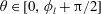$\unicode[STIX]{x1D703}\in [0,\unicode[STIX]{x1D719}_{l}+\unicode[STIX]{x03C0}/2]$ for $\unicode[STIX]{x1D719}_{l}\in [0,\unicode[STIX]{x03C0}/2]$ and $\unicode[STIX]{x1D703}\in [\unicode[STIX]{x1D719}_{l}-\unicode[STIX]{x03C0}/2,\unicode[STIX]{x03C0}]$ for $\unicode[STIX]{x1D719}_{l}\in (\unicode[STIX]{x03C0}/2,\unicode[STIX]{x03C0}]$ .

For the vertical displacement, the stabilities can be inferred from the derivative ${\dot{f}}$ : ${\dot{f}}>0$ corresponds to an unstable equilibrium while ${\dot{f}}<0$ corresponds to a stable equilibrium. By substituting equations (2.2), (2.15a–d ) and (2.16) into (2.14), the derivative ${\dot{f}}=\unicode[STIX]{x1D6FF}f_{net}^{v}/\unicode[STIX]{x1D6FF}h$ is given by

(3.14) $$\begin{eqnarray}\displaystyle {\dot{f}} & = & \displaystyle -\unicode[STIX]{x1D70C}gD-\unicode[STIX]{x1D70E}\sqrt{\unicode[STIX]{x1D705}}\left\{{\displaystyle \frac{\sqrt{\unicode[STIX]{x1D705}}R_{l}\cos \unicode[STIX]{x1D719}_{l}\sin \unicode[STIX]{x1D711}_{l}+\sin \left({\displaystyle \frac{\unicode[STIX]{x1D719}_{l}}{2}}+{\displaystyle \frac{\unicode[STIX]{x03C0}}{4}}\right)\sin \unicode[STIX]{x1D719}_{l}}{\left[\sqrt{\unicode[STIX]{x1D705}}R_{l}\cos \unicode[STIX]{x1D711}_{l}+\sin \left({\displaystyle \frac{\unicode[STIX]{x1D719}_{l}}{2}}+{\displaystyle \frac{\unicode[STIX]{x03C0}}{4}}\right)\right]\sin \left({\displaystyle \frac{\unicode[STIX]{x1D719}_{l}}{2}}+{\displaystyle \frac{\unicode[STIX]{x03C0}}{4}}\right)}}\right.\nonumber\\ \displaystyle & & \displaystyle \left.+\,{\displaystyle \frac{\sqrt{\unicode[STIX]{x1D705}}R_{r}\cos \unicode[STIX]{x1D719}_{r}\sin \unicode[STIX]{x1D711}_{r}+\sin \left({\displaystyle \frac{\unicode[STIX]{x1D719}_{r}}{2}}+{\displaystyle \frac{\unicode[STIX]{x03C0}}{4}}\right)\sin \unicode[STIX]{x1D719}_{r}}{\left[\sqrt{\unicode[STIX]{x1D705}}R_{r}\cos \unicode[STIX]{x1D711}_{r}+\sin \left({\displaystyle \frac{\unicode[STIX]{x1D719}_{r}}{2}}+{\displaystyle \frac{\unicode[STIX]{x03C0}}{4}}\right)\right]\sin \left({\displaystyle \frac{\unicode[STIX]{x1D719}_{r}}{2}}+{\displaystyle \frac{\unicode[STIX]{x03C0}}{4}}\right)}}\right\},\end{eqnarray}$$

where $D=x_{r}-x_{l}$ denotes the horizontal distance between two contact points. Because there are too many variables involved in ${\dot{f}}$ , only several representative quantities are studied, including the distance $D$ , the radii of curvature $R_{l}$ and $R_{r}$ . It is noted that the first term on the right-hand side of (3.14) is the same as the expression ${\dot{f}}$ for the case without surface tension. Then the surface tension effects on the vertical stability refer to the second term on the right-hand side of (3.14). In the second term, the effects at two contact points are independent and identical to each other, so that only the left side is taken into account.

Figure 10(a) shows the derivative ${\dot{f}}$ varying with the radii of curvature for the symmetric configurations (i.e. the right side is the mirror image of the left side with respect to $x=0$ ) for different contact angles, where $\unicode[STIX]{x1D719}_{l}$ and $x_{l}$ remain constant to keep the configuration unchanged (see the left inset). The additional diagrams for the mirror case of the origin configuration with respect to water line can be obtained by substituting $\unicode[STIX]{x1D703}$ with $\unicode[STIX]{x03C0}-\unicode[STIX]{x1D703}$ in figure 10(a). Assume without loss of generality that $\unicode[STIX]{x1D719}_{l}\in [0,\unicode[STIX]{x03C0}/2]$ . It is found that the smaller the radius of curvature, the better the stability of the floating body for $\unicode[STIX]{x1D703}\neq 0$ . For $\unicode[STIX]{x1D703}=0$ , equation (3.14) can be reduced to

(3.15) $$\begin{eqnarray}{\dot{f}}=-\unicode[STIX]{x1D70C}gD-\unicode[STIX]{x1D70E}\sqrt{\unicode[STIX]{x1D705}}\left[{\displaystyle \frac{\sin \unicode[STIX]{x1D711}_{l}}{\sin (\unicode[STIX]{x1D711}_{l}/2+\unicode[STIX]{x03C0}/4)}}+{\displaystyle \frac{\sin \unicode[STIX]{x1D711}_{r}}{\sin (\unicode[STIX]{x1D711}_{r}/2+\unicode[STIX]{x03C0}/4)}}\right],\end{eqnarray}$$

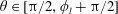and therefore the radius of curvature has no effect on the vertical stability of the floating body. For $\unicode[STIX]{x1D703}\in [0,\unicode[STIX]{x03C0}/2]$ , the vertical stability of floating body becomes better with the decrease of $\unicode[STIX]{x1D703}$ . For $\unicode[STIX]{x1D703}\in [\unicode[STIX]{x03C0}/2,\unicode[STIX]{x1D719}_{l}+\unicode[STIX]{x03C0}/2]$ , the vertical stability of floating body with $R_{l}\geqslant R_{c}$ (see the critical point $p_{c}$ in the right inset) becomes better with the decrease of $\unicode[STIX]{x1D703}$ , while the opposite is true for the floating body with $R_{l}<R_{c}$ . It is also found that from $R_{l}\sim 10^{-4}$ to $10^{-1}$ there is a dramatic change in the vertical stability, implying that $R_{l}>10^{-1}$ and $R_{l}<10^{-4}$ have pretty much the same effects of $R_{l}=\infty$ and $R_{l}=0$ , respectively.

In figure 10(b), the relation between the dimensionless parameters ${\dot{f}}/\unicode[STIX]{x1D70C}gD$ and the Bond number $Bo=\unicode[STIX]{x1D70C}gD^{2}/\unicode[STIX]{x1D70E}$ is presented. For macroscale bodies ( $Bo\gg 1$ ), the influence of surface tension is covered by the influence of gravity (see the horizontal dashed line). For microscale bodies ( $Bo\rightarrow 0$ ), only the effects of surface tension exist (see the inclined dashed line). For mesoscale bodies ( $Bo\sim 1$ ), the values of ${\dot{f}}$ vary continuously between the above two states, which may lead to the change of stability.

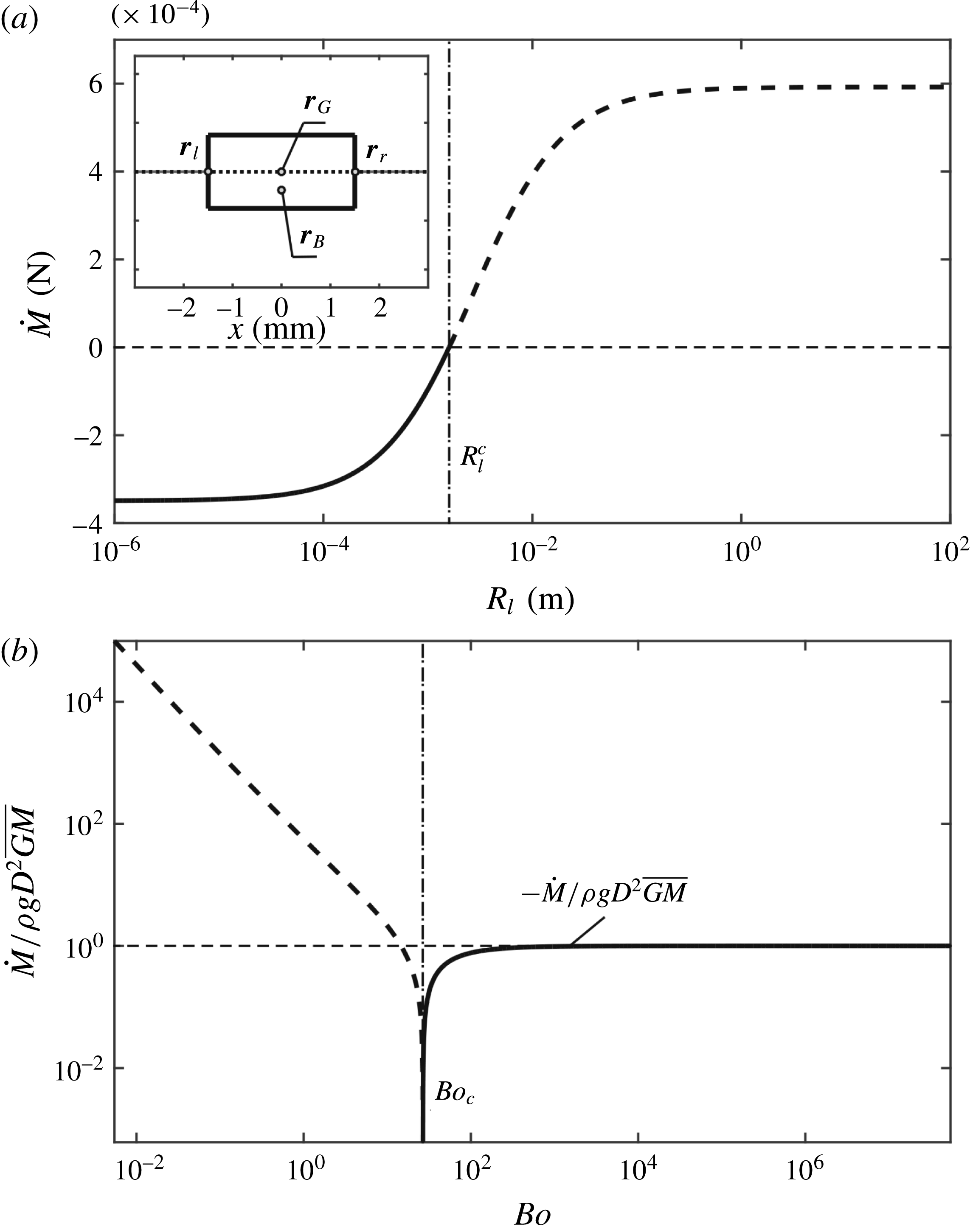
Figure 11. Surface tension effects on the rotational stability: (a) the effect of the radii of curvature and (b) the effect of the Bond number. The inset in (a) shows the configuration of the case (i) $\unicode[STIX]{x1D70C}_{s}=0.5\unicode[STIX]{x1D70C}$ , $\unicode[STIX]{x1D703}=\unicode[STIX]{x03C0}/2$ , $\unicode[STIX]{x1D706}=0.5$ and $a=1.5~\text{mm}$ for (a), while the configuration for (b) corresponds to the case (ii) $\unicode[STIX]{x1D70C}_{s}=0.5\unicode[STIX]{x1D70C}$ , $\unicode[STIX]{x1D703}=\unicode[STIX]{x03C0}/2$ , $\unicode[STIX]{x1D706}=0.5$ and $R_{l}=R_{r}=\infty$ . The thick dashed lines denote the unstable equilibria while the thick solid lines correspond to the stable equilibria, where the thin vertical dot-dash lines correspond to the critical values $R_{l}^{c}=1.598~\text{mm}$ and $Bo_{c}=\text{26.59}$ , respectively. The horizontal dashed line in (a) represents the critical value of ${\dot{M}}$ and the horizontal dashed line in (b) corresponds to the case without the surface tension effects.

For the rotational displacement, a specific equilibrium configuration of the rectangle (see the inset in figure 11 a) is considered to study the effects of surface tension on the rotational stability. It is well known that for a floating body without the surface tension effects the metacentric height ( $\overline{GM}$ ) is a measurement of its rotational stability (Biran Reference Biran2003). For a floating body under the surface tension effects, the derivative ${\dot{M}}$ can be used to determine the rotational stability. However, the expression of ${\dot{M}}$ is too complex to write here.

Figure 11(a) shows the derivative ${\dot{M}}$ varying with the radius of curvature $R_{l}$ for the specific equilibrium configuration (see the inset), where $R_{l}=R_{r}$ . The radii of curvature $R_{l}$ and $R_{r}$ at the contact points are varied artificially. Analogous to the vertical stability, the rotational stability will become better for smaller radii of curvature. Results show that in the range $R_{l}\sim 10^{-4}$ to $10^{-1}$ there is a dramatic change in the rotational stability, which is similar to the result of vertical stability, lead to a change in the rotational stability. Figure 11(b) shows the effect of size on the rotational stability. For comparison with the case without surface tension, the dimensionless parameter ${\dot{M}}/\unicode[STIX]{x1D70C}gD^{2}\overline{GM}$ is selected as the ordinate, because ${\dot{M}}=-\unicode[STIX]{x1D70C}gD^{2}\overline{GM}$ for the case without surface tension. The metacentric height is given by

(3.16) $$\begin{eqnarray}\overline{GM}={\displaystyle \frac{5D}{96}},\end{eqnarray}$$

where $D=2a$ is the characteristic length for the Bond number $Bo=\unicode[STIX]{x1D70C}gD^{2}/\unicode[STIX]{x1D70E}$ . It is found that when the Bond number is greater than 1000, the system tends towards the case without the surface tension effects. When the Bond number is less than 1, the gravity has no effect on the system.