


1 Introduction
Dynamic stall is a fundamental unsteady flow event that occurs when the apparent angle of attack (AoA) of a lifting surface is changed dynamically. Usually this is due to a wing being either pitched or oscillated, though it can also be caused by changes in the approach flow direction. This dynamic change in the AoA results in the formation of a strong vortex, i.e. the dynamic stall vortex (DSV), near the leading edge of the airfoil, which affects airfoil performance by delaying stall and increasing the maximum lift. It has been shown that the increasing circulation of the DSV lowers the pressure on the suction side of the airfoil, which increases the lift up to three times the static maximum (Gendrich Reference Gendrich1999). This lift benefit is only temporary as the DSV eventually convects away from the suction surface and the airfoil enters a traditional stall state. The unsteady lift has been shown to be advantageous in some cases like insect flight (Ellington et al. Reference Ellington, Berg, Willmott and Thomas1996; Dickinson, Lehmann & Sane Reference Dickinson, Lehmann and Sane1999) and ‘supermanoeuvrable’ aircraft (Graham Reference Graham1985; Brandon Reference Brandon1991). It can also be detrimental in other technological settings such as helicopter rotor dynamics (Carr, McAlister & McCroskey Reference Carr, McAlister and McCroskey1977).
Most early dynamic stall studies (e.g. Carr et al. Reference Carr, McAlister and McCroskey1977) focused on the dynamics of helicopter rotors. During forward flight the effective AoA of the rotor rapidly changes as it advances into and away from the free-stream flow during rotation. The changes in the apparent AoA result in a dynamic stall condition that creates highly unsteady loading on the rotor blades and effectively limits maximum forward flight speed of the helicopter. Dynamic stall is also an issue for turbomachinery and wind turbines because of unsteady large-magnitude blade loading conditions which can cause structural failures (McCroskey Reference McCroskey1982). Control methods have been proposed to delay or eliminate the DSV, but usually require active suction or blowing (Visbal Reference Visbal1991; Ekaterinaris Reference Ekaterinaris2002). One particularly interesting control study is that of Mai et al. (Reference Mai, Geissler, Kitcher, Bosbach, Richard and de Groot2008) which showed that dynamic stall can be controlled using passive, small-scale, leading-edge vortex generators, which are also commonly used as stall delay mechanisms for static scenarios.
The flippers of humpback whales (Megaptera novaeangliae) exhibit a unique geometry. Typically, the leading edges of nearly all aerodynamic lifting surfaces are smooth, both in nature and in modern technology, to maintain flow attachment along the aerodynamic surface. Humpback whales, however, have large leading-edge structures on their flippers (figure 1). Similar structures, termed tubercles, are not observed in other whale species. Early studies of the humpback whale flipper have suggested that the leading-edge tubercles act in a similar way to aircraft vortex generators (strakes) keeping the flow attached at high AoA (Fish & Battle Reference Fish and Battle1995).

Figure 1. Humpback whale flipper shape. Photo by Sho Hatakeyama (https://unsplash.com/photos/Cu6I_d8gw5A).
The hypothesis of the current work is that humpback whale tubercles generate streamwise vortices that delay the separation and convection of the DSV away from the suction surface of the airfoil. More specifically, that the tubercles of the humpback whale are passive dynamic stall control mechanisms that enable the high degree of manoeuvrability displayed by the humpback whale. If true, these structures could be used to delay dynamic stall to higher angles. This study investigates the effect of idealized leading-edge tubercles on an airfoil undergoing constant pitch rate motion to study the dynamics of the formation and convection of the DSV.
2 Background
Dynamic stall effects on helicopter rotors, and to a lesser extent on turbomachinery, were the common driving force behind early experiments on dynamic stall (Carr et al. Reference Carr, McAlister and McCroskey1977; McAlister, Carr & McCroskey Reference McAlister, Carr and McCroskey1978; McCroskey Reference McCroskey1982). During forward helicopter flight the effective AoA of a rotor blade rapidly changes as it advances into and away from the free-stream flow during rotation. Carr et al. (Reference Carr, McAlister and McCroskey1977) focused on a number of airfoil sections, but went into great detail on their results for the NACA 0012. That airfoil has since become one of the most commonly studied, but has one of the most complicated dynamic stall behaviour patterns of any of the airfoils used in dynamic stall testing. A complex combination of leading-edge separation and its interaction with trailing-edge separation dynamics is observed for this airfoil. Results show that flow reversal originating at the trailing edge reaches upstream 40 % of the chord on the suction side of the airfoil (Carr et al. Reference Carr, McAlister and McCroskey1977). When it reaches this point the flow reversal jumps forward near instantaneously to the leading edge of the airfoil. From this observation, Carr et al. (Reference Carr, McAlister and McCroskey1977) suggested that the dynamic stall mechanism of the NACA 0012 was an abrupt turbulent separation beginning around mid-chord. In static experiments, the NACA 0012 airfoil falls in a range where either leading-edge bubble bursting or mixed leading-edge/trailing-edge stall occurs. The leading edge of the NACA 0012 was sharpened and blunted to investigate leading-edge effects but no changes to the dynamic stall behaviour were observed (Carr et al. Reference Carr, McAlister and McCroskey1977). Boundary layer trips were also applied to compare laminar and turbulent separation bubbles, but again no difference was found in the stall behaviour (Carr et al. Reference Carr, McAlister and McCroskey1977). Factors identified by Carr et al. (Reference Carr, McAlister and McCroskey1977) as affecting dynamic stall behaviour, in order of maximum effect were: airfoil shape, pitching frequency/rate, pitching amplitude and Reynolds number. McCrosky’s (Reference McCroskey1982) review of unsteady flow behaviours extended the list of quantities affecting dynamic stall to include Mach number. The effect of the separation bubble on vortex formation was studied for the NACA 0012 airfoil by McAlister et al. (Reference McAlister, Carr and McCroskey1978). A boundary layer trip was used to transition the separation bubble at a range of oscillating amplitudes and frequencies, but this had little to no effect on dynamic stall. McAlister et al. (Reference McAlister, Carr and McCroskey1978) theorized that the DSV strength was directly related to the total circulation around the airfoil at the time of vortex formation. Also of note here is that the DSV formation was delayed with increased pitching frequency (McAlister et al. Reference McAlister, Carr and McCroskey1978).
Shih, Lourenco & Krothapalli (Reference Shih, Lourenco and Krothapalli1995), Oshima & Ramaprian (Reference Oshima and Ramaprian1997) and Pruski & Bowersox (Reference Pruski and Bowersox2013) all studied the dynamic stall phenomenon using particle image velocimetry to obtain quantitative measurements of the flow field. Results from these particle image velocimetry experiments showed that the DSV was not formed as a result of a Kelvin–Helmholtz instability (Shih et al. Reference Shih, Lourenco and Krothapalli1995). Secondary vorticity near mid-chord formed and may (Shih et al. Reference Shih, Lourenco and Krothapalli1995; Oshima & Ramaprian Reference Oshima and Ramaprian1997) or may not (Pruski & Bowersox Reference Pruski and Bowersox2013) affect the DSV. Oshima & Ramaprian (Reference Oshima and Ramaprian1997) defined this vortex as shear-layer vortex (SLV) and it was shown that it could reach up to 35 % of circulation found in the DSV (Shih et al. Reference Shih, Lourenco and Krothapalli1995).
Gendrich (Reference Gendrich1999) studied the formation of the DSV with highly resolved experimental data using molecular tagging velocimetry (MTV). The MTV technique can be effectively viewed as a molecular counterpart to particle image velocimetry. This experimental technique was also used in the current study and is explained in detail in later sections. Gendrich (Reference Gendrich1999) studied a NACA 0012 airfoil pitched at constant dimensionless pitch rates of  $\unicode[STIX]{x1D6FA}^{\ast }=0.1{-}0.4$, where
  $\unicode[STIX]{x1D6FA}^{\ast }=\dot{\unicode[STIX]{x1D6FC}}c/2U_{\infty }$, at a chord Reynolds number of 12 000 in a water tunnel. The spatial resolution in this experiment was
  $0.003c$ which allowed for detailed analysis of the leading-edge dynamics to be conducted. Low-Reynolds-number experiments were selected for ease of comparison to the numerical model of Choudhuri, Knight & Visbal (Reference Choudhuri, Knight and Visbal1994). Focus was placed on the leading-edge region to generate high-resolution data of the DSV formation process (i.e. up to the angle at which the DSV began to convect away from the airfoil surface). Extensive work was also done to show that the flow was highly repeatable and thus a candidate for phase averaging to airfoil pitch angle. Gendrich (Reference Gendrich1999) detailed specific formation angles and a highly resolved vortex structure, but did not measure the flow downstream of the DSV formation region.
Gendrich (Reference Gendrich1999) found that at low incidence angles the boundary layer remained attached to the airfoil surface but with increasing boundary layer thickness as a function of the AoA. A thin region of vorticity, with sign opposite to that of the boundary layer, formed underneath the primary vorticity along the airfoil surface in the recirculating region. Gendrich (Reference Gendrich1999) defined this flow condition as detached but not separated, where detached flow was defined as when ‘a thin region of opposite-sign vorticity is present under the primary shear layer’. Separated flow was defined as when the flow no longer followed the contours of the airfoil shape. When the flow detached, a ‘bulge’ formed near the leading edge which was associated with a growth in the reversed flow region. This reversed flow region induced the boundary layer flow back towards the airfoil surface cutting off the reversed flow region downstream. The bulge region near the leading edge is commonly referred to as the separation bubble, which sometimes is said to ‘burst’ forming the DSV (Carr et al. Reference Carr, McAlister and McCroskey1977). Around the time that the separation bubble formed, the reversed flow shear layer began to expand up into the flow away from the airfoil surface. The pressure gradients inside this bubble generated another thin layer of vorticity forming a three-layer vortical structure that had previously only been observed in the computational model of Choudhuri et al. (Reference Choudhuri, Knight and Visbal1994). The expansion of this third region of vorticity away from the airfoil pushes up the overlaying reversed flow region which in turn develops the full DSV along with secondary and tertiary vorticity regions. The results of Gendrich (Reference Gendrich1999) indicated that the source of the vorticity within the DSV was derived from the original airfoil boundary layer. Further this source continuously fed with vorticity from the leading edge during formation. A secondary vortex structure, originating from the first reversed flow region, was formed by vorticity from the reversed shear layer. A third vortex formed from the leading-edge vorticity interacting with the secondary vortex. The tertiary region of vorticity, which was near the surface underneath the secondary vortex, did not form a vortex-like structure but was the driving factor that pushed the reversed shear flow away from the surface forming the secondary vortex. Gendrich (Reference Gendrich1999) suggested that the formation of this tertiary region of reversed flow was the initiator of the secondary vortex which in turn pinched off the large DSV.
Numerical simulations and the experimental data of Gendrich (Reference Gendrich1999) were used to investigate the impact of pitch rate on DSV formation. Increased pitch rate resulted in a more compact leading-edge separation process that occurred closer to the leading edge at high pitch rates ( $\unicode[STIX]{x1D6FA}^{\ast }>0.2$; Gendrich Reference Gendrich1999). These results showed the formation of the thin reversed flow region near the leading edge can occur in two different ways: via the progression of the reversed flow from the trailing edge, or independently near the leading edge. The independent formation method was only observed for high pitch rates of
  $\unicode[STIX]{x1D6FA}^{\ast }>0.3$. The transition between these two stall mechanisms was evaluated computationally and observed to switch at around
  $\unicode[STIX]{x1D6FA}^{\ast }=0.2$. Vorticity was significantly higher for higher pitch rate cases and the vortex structures that formed were more compact and nearer the leading edge. Phase-averaged experimental results at high pitch rates proved to be an issue for observing the formation mechanisms due to decreased repeatability. Increases in small-scale structures and three-dimensional effects appeared to play a role in repeatability at higher pitch rates (Gendrich Reference Gendrich1999).
The frame of reference of the data presented may also have a significant effect on the results of the data (Gendrich Reference Gendrich1999). A common first method of rotating the airfoil into a rotating frame of reference is the transformation of rotating the coordinate system and velocity vectors to align with the airfoil. With this simple coordinate transformation, the vector magnitudes and angles remain the same with respect to the airfoil surface, but the airfoil surface retains a velocity from the pitching motion. This unwanted velocity of the airfoil surface can be eliminated with the addition of a solid-body rotation to the coordinate transformation developed by Gendrich (Reference Gendrich1999):
 $$\begin{eqnarray}\displaystyle & \displaystyle X=x\cos (\unicode[STIX]{x1D6FC})-y\sin (\unicode[STIX]{x1D6FC}), & \displaystyle\end{eqnarray}$$
 $$\begin{eqnarray}\displaystyle & \displaystyle Y=x\sin (\unicode[STIX]{x1D6FC})+y\cos (\unicode[STIX]{x1D6FC}), & \displaystyle\end{eqnarray}$$
 $$\begin{eqnarray}\displaystyle & \displaystyle \frac{U}{U_{\infty }}=\frac{U}{U_{\infty }}\cos (\unicode[STIX]{x1D6FC})-\frac{v}{U_{\infty }}\sin (\unicode[STIX]{x1D6FC})-2\unicode[STIX]{x1D6FA}^{\ast }Y, & \displaystyle\end{eqnarray}$$
 $$\begin{eqnarray}\displaystyle & \displaystyle \frac{V}{U_{\infty }}=\frac{u}{U_{\infty }}\sin (\unicode[STIX]{x1D6FC})+\frac{v}{U_{\infty }}\cos (\unicode[STIX]{x1D6FC})-2\unicode[STIX]{x1D6FA}^{\ast }X. & \displaystyle\end{eqnarray}$$
 Equations (2.1)–(2.4) use the pitch angle  $(\unicode[STIX]{x1D6FC})$, flow velocities
  $(u,v)$, free-stream velocity
  $(U_{\infty })$, dimensionless pitch rate and spatial locations of the velocity vectors. Note that here
  $x$ and
  $y$ are dimensionless
  $(x/c,y/c)$ and are left in the form shown in Gendrich (Reference Gendrich1999).
More recently, work by Visbal & Garmann (Reference Visbal and Garmann2017) computationally evaluated the dynamic stall of a NACA 0012 wing at low Reynolds number and at a lower pitch rate than used by Gendrich (Reference Gendrich1999). They observed a laminar separation bubble and determined that the breakdown of that flow feature preceded the onset of DSV formation. Visbal & Garmann (Reference Visbal and Garmann2017) also observed the SLV features noted by Shih et al. (Reference Shih, Lourenco and Krothapalli1995), Oshima & Ramaprian (Reference Oshima and Ramaprian1997) and Pruski & Bowersox (Reference Pruski and Bowersox2013).
One dynamic stall control study of particular relevance to the current work is one that used small vortex generators (Mai et al. Reference Mai, Geissler, Kitcher, Bosbach, Richard and de Groot2008). Small circular vortex generators (6 mm in diameter, 0.54–1.1 mm in height) were applied to the leading-edge area of an airfoil. The optimal location was found to be around  $0.17c$ on the pressure side of the airfoil, not on the suction side where one might naturally assume. The vortex generators were placed at
  $0.05c$ spacing along the span and tested for both light and deep dynamic stall. Mai et al. (Reference Mai, Geissler, Kitcher, Bosbach, Richard and de Groot2008) observed that lift hysteresis was reduced significantly during the reattachment phase of the motion. Reductions in lift hysteresis of up to 39 % were observed when the vortex generators were applied. Both drag and moment coefficients saw improvements of approximately 25 % during the downswing phase of the motion. The results were relatively independent of Mach number and pitching condition. These devices appeared to improve reattachment by energizing the boundary layer of the airfoil in a way similar to small tubercles on the humpback whale flipper. These results on the control of dynamic stall mimic some of the findings for humpback whale tubercles, where small tubercles were suggested to act as vortex generators (Borg Reference Borg2012).
The analysis of a humpback whale flipper as an aerodynamic/hydrodynamic shape was first performed by Fish & Battle (Reference Fish and Battle1995), where they discussed the tubercle structure on the leading edge of the flipper and its aerodynamic/hydrodynamic impact. The authors analysed a flipper recovered from a beached whale in coastal New Jersey. The flipper was roughly elliptic in shape with a slight backward sweep, had a span of 2.5 m and a wing area of approximately  $1.02~\text{m}^{2}$. The flipper also had a mean aerodynamic chord of 0.82 m, a thickness-to-chord ratio of 0.2–0.26 and an aspect ratio of 6.1, making it strikingly similar in size and shape to modern aircraft wings. The flipper dissected by Fish & Battle (Reference Fish and Battle1995) had a total of 11 tubercles on the leading edge, with tubercle height decreasing along the span. Cross-sectional slices of the flipper were compared with known aerodynamic airfoils and Fish & Battle (Reference Fish and Battle1995) found that the flipper closely resembled a NACA
  $63_{4}$-021 airfoil at mid-span. The function of the tubercles was assumed to be a passive stall control mechanism similar to vortex generators (strakes) on full-scale aircraft.
Humpback whales are known to hunt using a bubble-net technique in which they release bubbles while circling prey from below thereby corralling their prey. When the bubble net becomes small enough the whale turns into the middle of the net and surfaces with its mouth open capturing the prey. Bubble-net diameters vary based on specific prey animals from 1.5 up to 50 m. The minimum turning radius of a ‘typical’ humpback whale was estimated to be 7.4 m at a  $90^{\circ }$ bank angle using basic aerodynamic lift and drag assumptions. The authors explained the difference between their calculated minimum radius and field-observed minimum
  $({\sim}1.5~\text{m})$ in two separate ways: first that the humpback whale must be using its flippers as more than just static wings and overall manoeuvrability would be higher for an actual whale, and second that the tubercles may be having a beneficial aerodynamic/hydrodynamic effect.
The majority of the work that has been performed on tubercled airfoils has been focused on conditions at fixed AoA (i.e. static conditions). These studies have suggested that tubercles impact the flow through a combination of limiting spanwise flow (Watts & Fish Reference Watts and Fish2001; Miklosovic et al. Reference Miklosovic, Murray, Howle and Fish2004, 2007), re-energizing the flow by acting as vortex generators (Stanway Reference Stanway2006; Johari et al. Reference Johari, Henoch, Custodio and Levshin2007) and acting as vortex lift generators (Stanway Reference Stanway2006; Custodio Reference Custodio2008). A combination of these appears to be true depending on the dimensions of the tubercle. Small-amplitude tubercles tend towards acting as vortex generators, adding momentum to the flow and directly impacting the boundary layer (van Nierop, Alben & Brenner Reference van Nierop, Alben and Brenner2008; Hansen, Kelso & Dally Reference Hansen, Kelso and Dally2011). Very-large-amplitude tubercles impact the flow acting more as a delta-wing attachment to the leading edge and generating vortex lift (Custodio Reference Custodio2008). Vortex lift from large-amplitude tubercles was the likely cause of the flattening of the lift curve in the stall region with a constant post-stall lift above that of baseline airfoils (Miklosovic et al. Reference Miklosovic, Murray, Howle and Fish2004, 2007; Johari et al. Reference Johari, Henoch, Custodio and Levshin2007). Limiting of spanwise flow was present for tubercles of most sizes, excluding only the smallest tubercles, and had the greatest impact on finite-span studies (Miklosovic et al. Reference Miklosovic, Murray, Howle and Fish2004; Chen, Li & Nguyen Reference Chen, Li and Nguyen2012). More specifically, Miklosovic et al. (Reference Miklosovic, Murray, Howle and Fish2004) showed that the stall angle of their finite-span flipper-shaped wing was around  $\unicode[STIX]{x1D6FC}=17^{\circ }$ with a drop in lift from
  $C_{L}>1$ to
  $C_{L}<0.5$. However, for their tubercled wing, the lift deviated from the linear lift slope around
  $\unicode[STIX]{x1D6FC}=10^{\circ }$ but maintained a
  $C_{L}\approx 0.7$ past
  $\unicode[STIX]{x1D6FC}=12^{\circ }$. The lift coefficient on the tubercled wing never dropped below
  $C_{L}=0.6$ for any post-stall angles.
Numerous computational studies have reached similar conclusions. Their results showed lift and drag trends similar to those of experimental studies (Pedro & Kobayashi Reference Pedro and Kobayashi2008; Melipeddi, Mahmoudnejad & Hoffmann Reference Melipeddi, Mahmoudnejad and Hoffmann2011; Weber et al. Reference Weber, Howle, Murray and Miklosovic2011; Yoon et al. Reference Yoon, Hung, Jung and Kim2011), but many noted poor correlation to the lift and drag quantities observed in those experiments (Pedro & Kobayashi Reference Pedro and Kobayashi2008; Melipeddi et al. Reference Melipeddi, Mahmoudnejad and Hoffmann2011; Weber et al. Reference Weber, Howle, Murray and Miklosovic2011; Corsini, Delibra & Sheard Reference Corsini, Delibra and Sheard2013). Certain flow features were also commonly observed in these studies, such as: flow accelerating through trough regions (Melipeddi et al. Reference Melipeddi, Mahmoudnejad and Hoffmann2011; Yoon et al. Reference Yoon, Hung, Jung and Kim2011; Favier, Pinelli & Piomelli Reference Favier, Pinelli and Piomelli2012; Corsini et al. Reference Corsini, Delibra and Sheard2013; Skillen et al. Reference Skillen, Revell, Favier, Pinelli and Piomelli2013), spanwise flow inhibition (Pedro & Kobayashi Reference Pedro and Kobayashi2008; Yoon et al. Reference Yoon, Hung, Jung and Kim2011) and vorticity generated by the tubercles (Pedro & Kobayashi Reference Pedro and Kobayashi2008; Melipeddi et al. Reference Melipeddi, Mahmoudnejad and Hoffmann2011; Yoon et al. Reference Yoon, Hung, Jung and Kim2011; Favier et al. Reference Favier, Pinelli and Piomelli2012; Corsini et al. Reference Corsini, Delibra and Sheard2013; Skillen et al. Reference Skillen, Revell, Favier, Pinelli and Piomelli2013).
Little work has been performed on the dynamic motion of tubercled airfoils, but Borg (Reference Borg2012) showed promising preliminary results for improvements of control of dynamic stall. There is good reason to believe that beneficial effects from dynamic stall may be present for humpback whales. Segre et al. (Reference Segre, Mududzi, Meyer and Findlay2017) studied humpback whales in the wild and observed some interesting aspects of humpback whale behaviour: ‘immediately before opening their mouths, humpbacks will often rapidly move their flippers, and it has been hypothesized that this movement is used to corral prey’. They go on to suggest that the large flippers and dynamic motions might be used to generate significant lunging forces. Segre et al. (Reference Segre, Mududzi, Meyer and Findlay2017) applied suction cup digital recording tags to several humpback whales and were able to record two instances of what they called ‘hydrodynamically active flipper-strokes’. One such motion is of particular interest to the evaluation of flippers as dynamic, rather than static, lift generators. While the dynamic behaviour of humpbacks is obvious upon watching videos of the whales swimming, Segre et al. (Reference Segre, Mududzi, Meyer and Findlay2017) documented a clear case which can be evaluated aerodynamically. They recorded a rapid downward flipper stroke that rotated the flippers  $90^{\circ }$ in approximately 0.8 s. Given the conditions noted here and a few reasonable assumptions, this motion is easily shown to be in the range of the unsteady aerodynamic conditions encompassing dynamic stall.
The actuation motion observed by Segre et al. (Reference Segre, Mududzi, Meyer and Findlay2017), combined with the mean chord length of the humpback whale from Fish & Battle (Reference Fish and Battle1995) of 0.82 m, and an assumption of  $3~\text{m}~\text{s}^{-1}$ forward velocity of the whale, leads to a non-dimensional pitch rate of
  $\unicode[STIX]{x1D6FA}^{\ast }=0.21$. This result places the motion significantly above the threshold of
  $\unicode[STIX]{x1D6FA}^{\ast }>0.05$ with a peak AoA greater than the static stall angle, which defines the presence of a dynamic stall event. Segre et al. (Reference Segre, Mududzi, Meyer and Findlay2017) assumed a static lift maximum of 120 kN for this particular humpback.
One can easily perform a ‘back-of-an-envelope’ calculation to show the potential of dynamic, rather than static, lift to generate the large forces observed in humpback whales. The results of the dynamic stall study by Gendrich (Reference Gendrich1999) showed that the unsteady force on an infinite span airfoil was nominally three times the static lift maximum. If instead of using the  $C_{l,max}$ of the static case one conservatively assumes a more realistic
  $2C_{l,max}$ for the dynamic case, the whale could be generating an unsteady peak lunging force roughly equivalent to its own body weight. With this back-of-an-envelope result in mind, the evaluation of the effect of tubercles on dynamic stall becomes even more interesting.

Figure 2. Airfoil models.
The current work studies the effects of tubercles on a dynamically pitching airfoil at pitch rates in the deep dynamic stall range. Suction-side planar flow field data were collected to compare a tubercled airfoil to a baseline straight airfoil. Information derived from that dataset includes vortex formation angle, vortex convective path data and circulation. Vortex convective speed and the dynamic force generated by the vortex were inferred from these datasets. In particular, the circulation and convection characteristics of the DSV were used to infer the effects of the tubercles on the dynamic stall process.
3 Experimental methods
The airfoils created for the current study were designed with comparison to prior studies in mind. Tubercles applied to the airfoil had an amplitude of  $0.04c$ similar to the tubercles used in Miklosovic et al. (Reference Miklosovic, Murray, Howle and Fish2004) and the
  $0.05c$ ‘medium’ tubercles from Johari et al. (Reference Johari, Henoch, Custodio and Levshin2007). The span of the model was 36.8 cm (14.5 in) based on the width of a tunnel originally to be used for the study. This resulted in an aspect ratio of 3.1 for the current study. False walls were placed on both ends of the airfoil to limit end effects. An odd number of tubercles (13) was selected so that the middle tubercle would align to the centreline of the water tunnel (figure 2). The wavelength of the tubercles was approximately
  $0.24c$ which closely matches that of (Johari et al. Reference Johari, Henoch, Custodio and Levshin2007) while maintaining spanwise symmetry for mounted model.
Airfoils with leading-edge tubercles can be designed either by sinusoidally stretching/shrinking the leading edge or by scaling of the chord length of the airfoil data points with a sinusoidal function of amplitude and wavelength. Scaling the data points to a local chord maintains the airfoil profile at all span locations; however, this strategy changes the maximum thickness and chordwise location of the maximum thickness point resulting in waviness on the top surface of the airfoil. Stretching of the leading edge eliminated this by adjusting data points ahead of the peak thickness  $(0.3c)$ as a function of the local chord length. This method resulted in a uniform airfoil thickness and shape aft of
  $0.3c$ with the caveat that the airfoil cross-sectional shape changes and is only pure at specific spanwise locations. The chord length, and airfoil shape, for this airfoil was defined at the location midway between the peak and trough. The current work used the second strategy to maintain a uniform maximum thickness and location.
The overall thickness of the airfoil has been shown not to change the effect of the tubercles (Chen et al. Reference Chen, Li and Nguyen2012). A NACA 0012 airfoil section was selected for the design to enable comparison to the dynamic stall work of Gendrich (Reference Gendrich1999). While prior studies selected airfoils that more closely matched the humpback whale flipper cross-section (Fish & Battle Reference Fish and Battle1995; Johari et al. Reference Johari, Henoch, Custodio and Levshin2007), the current study used an unmodified NACA 0012 airfoil with the same span and chord length as used by Gendrich (Reference Gendrich1999), but lacking tubercles, as a baseline along with the modified NACA 0012 airfoil. Comparisons to the high-resolution leading-edge dynamic stall data in Gendrich (Reference Gendrich1999) also drove other key experimental and model parameters. The mean chord length  $(c=12~\text{cm})$, free-stream velocity
  $(U_{\infty }=10~\text{cm}~\text{s}^{-1})$, Reynolds number
  $(Re_{c}=12\,000)$ and non-dimensional pitch rates (
 $\unicode[STIX]{x1D6FA}^{\ast }=0.1$, 0.2, 0.4) were selected to match those in Gendrich (Reference Gendrich1999).
The models were three-dimensionally printed with a precision of 0.1 mm in three pieces using a Viper Si2® SLA system with DSM 11120 epoxy resin. The models were assembled, sanded and painted a matte black finish to minimize surface reflections. The planar flow measurements were recorded for the modified airfoil at the planes shown in figure 3. The baseline case was measured at the midspan location. The peak and trough planes will be primarily discussed in this paper, along with the baseline NACA 0012 measurement plane.

Figure 3. Tubercled airfoil data planes.
The current experiments utilize a constant pitch-up and hold motion. The wing was pitched up from  $0^{\circ }$ to
  $55^{\circ }$ at a constant pitch rate and held at the maximum angle for several convective times to allow the DSV to convect downstream. The dynamic pitching motion was controlled by a Galil DMC 40-20 servocontroller with a 4000 count per revolution servo motor. Encoder motion data from the experiments were analysed for sources of error in the pitch angle of the airfoil. The data acquisition frequency of the system was limited to 5 Hz due to laser and camera limitations. The previous work of Gendrich (Reference Gendrich1999) has shown that the results are repeatable from run to run and therefore the temporal resolution was increased by phase-averaging the results from multiple experimental runs in the following way. The start of the pitching motion of the airfoil was controlled with respect to the laser and camera operation. For the
  $\unicode[STIX]{x1D6FA}^{\ast }=0.1$ experiments, a series of 10 different start time delays, with respect to the start of motion, were used. The data from the different runs were phase-averaged with respect to the airfoil angle to provide an effective data rate of 50 Hz. For the higher pitch rates (
 $\unicode[STIX]{x1D6FA}^{\ast }=0.2$, 0.4) five start time offsets were used and phase-averaged for an effective data rate of 25 Hz. The resulting angular resolution of the data was approximately
  $0.19^{\circ }$ for
  $\unicode[STIX]{x1D6FA}^{\ast }=0.1$,
  $0.73^{\circ }$ for
  $\unicode[STIX]{x1D6FA}^{\ast }=0.2$ and
  $1.47^{\circ }$ for
  $\unicode[STIX]{x1D6FA}^{\ast }=0.4$. The lower angular resolution for the higher pitch rates was a combination of the reduced data rate and the significant increases in angular velocity of the airfoils. The timing presented here is normalized time
  $(t^{\ast }=tU_{\infty }/c)$ with the start of the pitching motion defining
  $t^{\ast }=0$.
The average control error, measured by comparing encoder position and the command position, varied as a function of pitch rate. Larger control errors were observed during the accelerative phase, as expected due to the effects of starting motion. The average control error for the entire pitching motion was small (see table 1). Figure 4 shows the control–response curves for the different pitch rates tested ( $\unicode[STIX]{x1D6FA}=0.1$, 0.2, 0.4) with figure 4(b) showing the accelerative region. Oscillations in the motion were observed that worsened with increased pitch rate, but typically dampened out before
  $\unicode[STIX]{x1D6FC}=10^{\circ }$. Past work (e.g. Gendrich Reference Gendrich1999) showed the flow dynamics was insensitive to these small deviations in the controller motion.

Figure 4. Control–response curves for (a) full pitching motion and (b) accelerating region.
Table 1. Motion control errors.

Whole-field planar velocity measurements were made using MTV. This is a non-intrusive optical flow measurement technique that uses a chemical tracer dissolved in a fluid that phosphoresces when excited by the appropriate wavelength of laser light. A combination of  $1.0\times 10^{-4}~\text{M}$
 $\text{g}_{1}\unicode[STIX]{x1D6FD}$-cyclodextrin, 0.05 M cyclohexanol and a solution of 1-bromonaphthalene was pre-mixed in the water tunnel. The bromonaphthalene acts as the lumophore and phosphoresces when excited by a fourth-harmonic Nd:YAG laser
  $(\unicode[STIX]{x1D706}=266~\text{nm})$. However, the phosphorescence is quenched by the presence of dissolved free oxygen in water. The cyclodextrin acts as a molecular ‘cup’ in which the bromonaphthalene can reside while the cyclohexanol bonds to the cyclodextrin cup acting as a cap and enclosing the bromonaphthalene inside. This chemical combination isolates the lumophore from the free oxygen dissolved in the water allowing it to phosphoresce with a lifetime of approximately 3–5 ms. The development of this MTV supramolecule and its application to fluid flow measurements are described in Gendrich, Bohl & Koochesfahani (Reference Gendrich, Bohl and Koochesfahani1997).

Figure 5. (a) Undelayed MTV image  $t=t_{0}$. (b) Delayed MTV image
  $t=t_{0}+3.5~\text{ms}$. (c) Resulting displacement vector field.
Quantitative optical velocity measurements require that the displacement of fluid regions be determined over a known time. In this work, a pulsed Nd:YAG laser (5 Hz, 266 nm) was used to excite the bromonaphthalene into a phosphorescent state. A series of intersecting laser lines were used to ‘tag’ the fluid with discrete intersections. Two images were taken in rapid sequence where the first image was taken immediately after laser firing (figure 5a) and the second image at some specified time later (i.e. the delay time,  $\unicode[STIX]{x0394}t$) (figure 5b). Images were captured using a PCO Dicam Pro CCD camera with a
  $1280\times 1024$ pixel resolution. The camera was oriented so that the longer axis of the image (1280 pixels) was aligned with the flow direction. An 80 mm Nikon lens was used to capture all the MTV images. The delay time for all MTV image pairs in this work was
  $\unicode[STIX]{x0394}t=3.5~\text{ms}$ to limit the maximum displacement between images to less than 10 pixels as recommended by Gendrich & Koochesfahani (Reference Gendrich and Koochesfahani1996). Laser intersection angles were nominally
  $90^{\circ }$ to reduce error in the measurements also as per Gendrich & Koochesfahani (Reference Gendrich and Koochesfahani1996).
Image pairs were converted into displacement fields using the direct correlation method described in Gendrich & Koochesfahani (Reference Gendrich and Koochesfahani1996) in the following way. Each grid intersection was identified in the undelayed images and a small region ( $21\times 21$ pixels) was defined around each intersection in the undelayed images. These subregions were then moved individually around the delayed image to determine the correlation field. The location of the maximum correlation for each subregion was taken as the displacement for that particular intersection. The velocity was found by dividing the displacement for a particular intersection by
  $\unicode[STIX]{x0394}t$. This provides a Lagrangian measurement of the velocity which is then taken to exist at the midpoint location between the undelayed and delayed intersections (figure 5c).
Two fields of view were used to increase the spatial extent of the measurements in this work. The two fields of view were overlapped to allow for alignment of the full velocity field. Locations of the laser intersections were shifted within each field of view for each of the 25 repeated trials to increase the effective spatial resolution of the data. The final spatial resolution was approximately 1 mm  $(0.008c)$ with a total field of view of approximately
  $17~\text{cm}\times 14~\text{cm}$.
The MTV data are typically irregularly spaced. The irregularly spaced data results were mapped onto a regularly spaced grid using the polynomial fitting technique described by Cohn & Koochesfahani (Reference Cohn and Koochesfahani2000). Vorticity was calculated based on this regular grid mapping of the data, using a second-order finite difference calculation. Circulation was calculated by integrating the vorticity field over a specified spatial area. The spatial area for the integration was allowed to vary with time based on the instantaneous measurement of the vortex core radius. This was done to accommodate the increasing size of the DSV as circulation was added from the leading edge.
The error in the velocity measurements is directly related to the error in the correlation process (i.e. the error in the determination of the displacement). A series of 100 undelayed images, with over 55 000 vectors, were correlated against an averaged image of all the undelayed images for that case. This, in effect, determined the error level in the displacement based on all system uncertainties including camera noise, tagging line orientation, tagging line width, etc. The vectors at each grid intersection were averaged to determine the average error in displacement at each of approximately 550 grid intersections. The 95 % error level was calculated using this method to be 0.05 pixels. This pixel error, when converted to an error in velocity, based on the image magnification and delay time, was found to be  $0.24~\text{cm}~\text{s}^{-1}$. It is noted that the error in the velocity measurement assumes that the delay time was known exactly. The jitter in the timing of the system was several orders of magnitude lower than the delay times used and therefore not significant. Error in the vorticity calculations was estimated to be
  $2.14~\text{s}^{-1}$ based on the analysis described in Bohl & Koochesfahani (Reference Bohl and Koochesfahani2009).
4 Results
4.1 Baseline NACA 0012
Results for the baseline NACA 0012 airfoil were consistent with observations in previous studies by Carr et al. (Reference Carr, McAlister and McCroskey1977), Gendrich (Reference Gendrich1999) and others. The case shown in figure 6 is that of  $\unicode[STIX]{x1D6FA}^{\ast }=0.1$, which was the lowest reduced frequency and the best temporally resolved case investigated. For ease of viewing, the vector maps in figures 6–8 show only every eighth vector of the datasets. The origin of the data presented is set such that
  $(x,y)=(0,0)$ is located at the pitching axis and corresponded to the
  $\frac{1}{4}$ chord location of the airfoil.
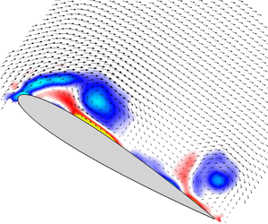
The flow remained attached near the leading edge at  $\unicode[STIX]{x1D6FC}=15^{\circ }$, which is higher than the static stall angle. The velocity field showed separation and reverse flow was present near the trailing edge. This region grew in thickness and advanced towards the leading edge as the AoA,
  $\unicode[STIX]{x1D6FC}$, increased. Trailing edge vortices also formed through the pitching motion. By
  $20^{\circ }$, a distinct region of vorticity along the airfoil surface was observed near the leading edge as the DSV began to form. When the airfoil reached
  $25^{\circ }$ the DSV had fully formed into a coherent vortex, though the DSV appeared to be continually strengthened from the leading-edge vorticity to angles greater than
  $\unicode[STIX]{x1D6FC}=40^{\circ }$. A SLV formed nominally at the 60 % chord location. A secondary vortex formed below the DSV and could be clearly observed at
  $\unicode[STIX]{x1D6FC}=25^{\circ }$ as a strong region of positive vorticity. As the pitching motion continued, the DSV grew in strength while the SLV convected towards the trailing edge. The secondary vortex grew in strength and size with increasing pitch angle inducing the DSV to move away from the airfoil and convect downstream. Evidence of a tertiary recirculating region below the secondary vortex was also observed at
  $\unicode[STIX]{x1D6FC}=30^{\circ }$. This tertiary region of vorticity has been theorized as the cause of upward growth of the secondary vortex and pinch-off the the DSV (Gendrich Reference Gendrich1999). These results are consistent with those of prior studies of dynamic stall formation (Carr et al. Reference Carr, McAlister and McCroskey1977; Gendrich Reference Gendrich1999), DSV formation angle (Gendrich Reference Gendrich1999) and flow features such as the SLV (Shih et al. Reference Shih, Lourenco and Krothapalli1995; Oshima & Ramaprian Reference Oshima and Ramaprian1997; Pruski & Bowersox Reference Pruski and Bowersox2013; Visbal & Garmann Reference Visbal and Garmann2017).

Figure 6. Baseline dynamic stall flow field.
4.2 Tubercled airfoil
The application of tubercles to the airfoil significantly changed the formation behaviour and physics of the dynamic stall process. Figure 7 shows the flow field results for the data plane on the peak of a tubercle. The baseline airfoil profile is overlaid in grey for spatial comparison while the forward protrusion of the tubercle (i.e. the actual airfoil leading-edge shape) is shown shaded black. At low pitch angles ( $\unicode[STIX]{x1D6FC}=15^{\circ }$,
  $20^{\circ }$), the boundary layer separation near the trailing edge and secondary reverse flow underneath it were more pronounced than for the baseline. The upstream advance of that reverse flow region was inhibited on this plane, with no forward progression of the trailing-edge separated flow region observed. Unlike the baseline case, a roll up of the vorticity near the leading edge into the DSV did not occur. Instead, a distinct region of compact vorticity formed along the surface near mid-chord while the flow remained attached forward towards the leading edge (
 $\unicode[STIX]{x1D6FC}=25^{\circ }$). While this region of vorticity could be thought of as the DSV, it was distinctly different from the more typical ‘leading-edge vortex’ nature of the DSV for the baseline case. The leading-edge flow attachment was observed at angles greater than
  $\unicode[STIX]{x1D6FC}=30^{\circ }$. This behaviour extended to high angles where the feeding vorticity for the DSV left the leading edge more in line with the free-stream flow direction when compared to the baseline.

Figure 7. Tubercled airfoil peak plane dynamic stall flow field.

Figure 8. Tubercled airfoil trough plane dynamic stall flow field.
Comparing the baseline (figure 6) and peak of the tubercled airfoil (figure 7), other significant differences existed between the two, the most notable of which were formation angle, vortex strength and vortex shape. At  $\unicode[STIX]{x1D6FC}=25^{\circ }$, the DSV was clearly observed on the baseline airfoil while only initial indications of a DSV and secondary recirculating region below it were seen on the peak plane. The strong reverse flow region that formed beneath the DSV did not separate or ‘erupt’ from the surface (figures 6 and 7 at
  $35^{\circ }$) for the peak plane. Further this reverse flow region did not develop a secondary vortex for the peak plane. Feeding vorticity from the leading edge was noticeably discontinuous from the leading edge to the vortex region (figure 7;
  $\unicode[STIX]{x1D6FC}=30^{\circ }$). The data recorded in this study were planar and thus out-of-plane motion, which is known to be present for the static case with tubercles (Watts & Fish Reference Watts and Fish2001), may have been the source of apparent discontinuities observed in vorticity. Compared to the baseline, the DSV formed later in the motion, further downstream along the airfoil chord, had a more elliptic shape and appeared to be more diffuse.
Flow measurements over the trough of the tubercle showed stark differences from the baseline and the peak plane of the tubercled airfoil. Figure 8 shows the trough plane flow field with the baseline airfoil shape again outlined in grey for reference and the tubercled airfoil trough in black. Key differences observed for this data plane were: an earlier formation of the DSV and a lack of secondary vortex formation from the reverse flow under the DSV, the DSV vortex formation location and its convective path. First, the leading-edge vorticity at this plane began to pinch off and roll up into a vortex at much lower angle than the baseline. The DSV, not observed until  $\unicode[STIX]{x1D6FC}\approx 20^{\circ }$ for the baseline, was apparent by
  $\unicode[STIX]{x1D6FC}=15^{\circ }$ in the trough of the tubercled airfoil. In addition to early formation angle, the DSV formed close to the leading edge and rolled up into a notably strong vortex in this region. However, that compact vortex structure was short-lived as by
  $\unicode[STIX]{x1D6FC}=30^{\circ }$ the DSV had convected to mid-chord and diffused significantly (figure 8). At
  $\unicode[STIX]{x1D6FC}=30^{\circ }$, the centre of rotation of the DSV was in approximately the same location as the DSV on the peak plane (figures 7 and 8).
Compared to the baseline, the DSV formed on the trough plane was more diffuse and feeding vorticity from the leading edge was at a steeper angle with respect to the airfoil surface. In this case, vorticity shed from the leading edge during the pitching process was almost perpendicular to the airfoil. On the baseline airfoil this feeding vorticity was more aligned with the free-stream flow and was almost in line with the free stream on the peak plane.
4.3 Vortex formation angle
One key aspect to the dynamic stall process is the determination of the angle at which the DSV begins to form. Determination of the formation angle of the DSV in a quantitative manner is challenging and limited by temporal and spatial resolution as well as by the ability to define the presence of a vortex. Two quantitative techniques were used to determine the vortex formation angle in this work. First, the application of streamlines to the flow field was used to identify the first frame that showed the spiraling flow behaviour typically associated with a vortex. Second, the presence of secondary vorticity is known to be the driver for pushing the DSV up from the airfoil surface (Gendrich Reference Gendrich1999). The angles at which secondary vorticity and spiraling streamlines were first observed are shown in table 2. One major consideration to evaluating the results of each of these methods is their heavy dependence on the temporal and spatial resolution of the data. In essence, the values presented in table 2 are reflective of the angles at which a DSV can first be observed at the data resolution from these experiments. The actual formation angle will occur between this angle and the prior measurement angle. These results will be likely to lag experiments with higher temporal resolution. Spatial resolution will also affect the observation time of the DSV formation as finer spatial resolution allows for a more precise picture of the velocity and vorticity fields to be observed. The formation angle of the baseline results was found to lag those of the experiments done by Gendrich (Reference Gendrich1999), but more closely match the computational results in the same study. The goal of that study, which had both higher spatial and temporal resolution, was to investigate the early formation of the DSV. The focus of the current study was more global and so spatial resolution near the airfoil surface was sacrificed, somewhat limiting the observation of vortex structures until they were sufficiently large. However, the current results provide trends in the formation angle between cases.
The results show that the DSV formed earliest in the trough of the tubercled airfoil and then progressively increased towards the peak plane. The baseline results showed a formation angle nominally the same as for the near-trough plane and significantly earlier than for the near-peak and peak planes. These results are consistent with what was observed in the full flow field results (figures 6–8). The methods for determining formation angle agreed well, with the only discrepancy occurring for the baseline. One factor likely causing these methods to converge for the tubercled airfoil is the eruption-like behaviour of DSV formation on the modified wing versus the roll-up behaviour of the baseline DSV. While the DSV on the trough plane formed earlier than the baseline, between  $0.7^{\circ }$ and
  $2.5^{\circ }$ earlier depending on method, the DSV on the peak plane formed significantly later in the pitch motion,
  $5.4^{\circ }{-}7.1^{\circ }$ later than the baseline. Using the data in table 2, the mean formation angle of the DSV on the tubercled airfoil was
  $\unicode[STIX]{x1D6FC}=21.7^{\circ }$ using the streamlines method and
  $\unicode[STIX]{x1D6FC}=21.4^{\circ }$ using secondary vorticity. A linear average of the formation angle is unlikely to reflect the intricacies of the spanwise flow on the tubercled airfoil. Instead it suggests that taken as a whole, the DSV formation is delayed on the tubercled airfoil with the peak and trough planes bounding the formation behaviour.
Table 2. Vortex formation angle.

4.4 Vortex tracking and convective path
The convective path of the DSV after formation impacts the lift and drag characteristics of the airfoil depending on proximity (Carr et al. Reference Carr, McAlister and McCroskey1977). The vortices were identified and tracked in the present case using the  $\unicode[STIX]{x1D6E4}_{1}$ criteria defined by Michard et al. (Reference Michard, Graftieaux, Lollini and Grosjean1997). Here
  $\unicode[STIX]{x1D6E4}_{1}$ is calculated using the velocity field data and the equation
 $$\begin{eqnarray}\unicode[STIX]{x1D6E4}_{1}(P)=\frac{1}{N}\mathop{\sum }_{S}\frac{(PM^{\wedge }U_{M})z}{\Vert PM\Vert \Vert U_{M}\Vert }=\frac{1}{N}\mathop{\sum }_{S}\sin (\unicode[STIX]{x1D703}_{M}).\end{eqnarray}$$
 Equation (4.1) calculates the average angle between the position vector from the calculation point and velocity vector of all measurement points in a user-defined region. The value of  $\unicode[STIX]{x1D6E4}_{1}$ is limited by
  $\pm 1$ (
 $\unicode[STIX]{x1D703}_{M}=90^{\circ }$) with the sign of
  $\unicode[STIX]{x1D6E4}_{1}$ describing the direction of rotation and a magnitude of 1 indicating a true circular motion of the velocity field around the analysis location. Here
  $\unicode[STIX]{x1D6E4}_{1}$ was chosen for tracking the vortices because the centre of rotation was found to be well defined even for the diffuse DSV. The spatial tracks of the DSV for the baseline and tubercled airfoils are shown in figure 9, with near-peak and near-trough plane data excluded. Velocity field data from these intermediary planes are not shown in this paper because of their similarity to the peak and trough plane data. All data in this section are shown in the airfoil frame of reference as the location of the DSV relative to the airfoil is important when determining relational effects. Recall that the origin location was taken at the pitching axis, the
  $\frac{1}{4}$ chord location.
Figure 9 shows that the baseline DSV formed forward of the  $\frac{1}{4}$ chord pitching axis and moved towards the trailing edge before convecting away from the airfoil surface. The baseline DSV moved towards the trailing edge up to
  $x_{AF}/c\approx 0.4$, roughly 65 % from the leading edge, before convecting away from the airfoil. At later times the baseline DSV convected upstream towards the leading edge reaching
  $x_{AF}/c\approx 0.3$ before again moving towards the trailing edge and drifting out of the field of view. In the trough plane of the tubercled airfoil, the DSV also formed near the leading edge, just slightly ahead of the baseline DSV formation location. However, the trough DSV lingered near the leading edge before moving quickly towards the trailing edge to align with and convect along the same path as the peak plane DSV, which formed behind the pitching axis. On the tubercled airfoil the DSV moved away from the airfoil surface around
  $x_{AF}/c\approx 0.3$ and did not exhibit the upstream motion exhibited by the baseline DSV.
Tracking the DSV as a function of time,  $t^{\ast }=tU_{\infty }/c$, allows for comparison of the location of the DSV across tubercled airfoil planes, answering the question of where the DSVs are at the same time in the pitching motion. Normalized time was used here instead of pitch angle as it allows tracking of the DSV after the pitching motion stopped. Figure 10 shows the
  $x_{AF}/c$ and
  $y_{AF}/c$ location of the DSVs for the different planes. Baseline and trough plane DSVs were formed at similar times while the peak plane DSV formed at a much later time. The data showed that there was spatial convergence of the DSV location of the peak and trough planes at around
  $t^{\ast }=2.75$, after which the DSV on the tubercled airfoil was nominally aligned across the span. This was notable given the differences in the flow conditions at the different locations on the tubercle geometry. The baseline DSV exhibited the greatest spatial variation throughout its convection where the baseline moved up and downstream in the flow more than the tubercled airfoil DSV.

Figure 9. Dynamic stall vortex tracking results.

Figure 10. Dynamic stall vortex tracking and convective path.
The vortex tracking data also allowed for the calculation of DSV convective velocity. Convective velocity was calculated by fitting the vortex location in time for both  $x_{AF}$ and
  $y_{AF}$ directions and then differentiating the fit. Twenty neighbouring data points (10 before and 10 after the current location) were used in the fit for each measurement time, generating the data in figure 11. All cases showed fluctuation in the convective velocities indicating that the formation and convection process was dynamic. Consider first the baseline case. After formation, the DSV moved away from the airfoil. Local peaks in
  $V_{conv,AF}$ indicate that this process was dynamic as the vortex accelerated and decelerated during this process. The maximum acceleration began to occur at
  $t^{\ast }=3.0$ after which the convective speed reached a maximum of
  $V_{conv,AF}\approx 0.6U_{\infty }$. The DSV continued to move away from the surface, though the rate decreased. The convective speed in the
  $x$ direction,
  $U_{conv,AF}$, highlighted the forward/backward motion of the DSV relative to the pitching location. The convective speeds in this direction were smaller and oscillated about zero. The convective speed away from the airfoil
  $(V_{conv,AF})$ was always positive but significantly less than the free-stream speed, of the order of 30 % of
  $U_{\infty }$. Speed in the chordwise direction
  $(U_{conv,AF})$ fluctuated about zero.
A peak in the convective velocity of the baseline DSV occurred around  $t^{\ast }=3.75$ and decelerated after that time. The convective velocity exceeded 60 % of that of the free stream for the baseline DSV at this point. At that time on the tubercled airfoil the opposite effect was noticed, with a local minimum in convective speed. While the speed of the DSVs on the tubercled airfoil tended to oscillate more, their convective speed remained lower than that for the baseline. These results also show that after the alignment motion of the trough DSV to match the location with the peak DSV, the trough DSV led the motion with a slight phase shift between the peak and trough. Despite the unique motion of the tubercled airfoil DSV, the mean convective velocity of the tubercled airfoil DSV was lower than that of the baseline.

Figure 11. Dynamic stall vortex convective velocity.
4.5 Circulation
Results so far have shown that, compared to a baseline airfoil, a tubercled airfoil generated DSVs in different locations, with different shapes and different convective behaviour. Changes in the dynamic lift and drag on the airfoil models were of interest to the current study, but lift and drag were not directly measured. Prior studies have shown that the dynamic lift generated in the dynamic stall process is caused by the strength of the low-pressure DSV and its proximity to the suction side of the airfoil (Carr et al. Reference Carr, McAlister and McCroskey1977; McCroskey Reference McCroskey1982). Fundamental differences in the flow were the primary focus of the current study, but inferences on the dynamic lift can be made from quantifying the circulation of the DSV. By comparing the circulation observed in Gao, Wei & Hrynuk (Reference Gao, Wei and Hrynuk2018) with the dynamic lift measured in Gendrich (Reference Gendrich1999) there is a strong correlation between dynamic lift and circulation of the DSV. This shows that the strength of the vortex, as quantified through the circulation, correlates with the dynamic lift generated on the airfoil.
Circulation is usually calculated from data either by summing the vorticity over the area of the vortex or by performing a line integral around the edge of the vortex. In both cases, calculating the circulation of a vortex is difficult to do as one must identify the outer edge of the vortex, which is hard to define. In this work the circulation was calculated in the same manner for all cases so that comparisons could be made. Circulation presented here is the circulation of only the DSV and was calculated as the sum of DSV vorticity within a varying radius in the following way. At each time, the radius of the vortex was calculated using the radius of gyration of the distributed vorticity in the manner described in Bohl & Koochesfahani (Reference Bohl and Koochesfahani2009). The circulation was then obtained by summing the vorticity over an area using  $1.75r_{core}$. This factor was used as it was found to define a circular area that was just slightly larger than the observed vorticity field of the DSV. The vorticity of the secondary vortex, which was of opposite sign compared to the DSV, was not included in the calculation to isolate the properties of the DSV.
Comparing the baseline and tubercled airfoil DSV circulations shows a significantly higher circulation for the tubercled airfoil at all planes compared to the baseline (figure 12). While the baseline and trough DSVs formed at similar times, the trough DSV exhibited higher circulation levels than the baseline, in part due to a plateau in circulation for the baseline around  $t^{\ast }=2$. This initial plateau in circulation was not observed on the trough although there was a decreased rate of growth around
  $t^{\ast }=2$ for that plane. Peak plane DSV circulation showed a similar trend despite a later formation time. A plateau in circulation occurred for the tubercled airfoil data around
  $t^{\ast }=2.75$, but was more pronounced for trough data. Circulation for the peak plane of the tubercled airfoil grew almost linearly up to a peak normalized circulation near 3.8 with other tubercled airfoil data having maximum circulation around 3.25. The second plateau in circulation occurred later for the baseline and maximum circulation was around 2.5. While the circulation appears to be increasing at the last data point, the data shown include only data where the entire DSV was inside the measurement field of view. All three cases shown exhibit regions of linear growth in the circulation with time. The slopes of these regions were computed using a linear fit and are also shown in figure 12. The growth rate in the circulation was similar for all measurement planes on the modified airfoil and nominally double the baseline growth rate. Further, while there were minor differences, the growth rate of the circulation was nominally doubled for the modified airfoil versus the baseline airfoil in these regions.

Figure 12. Dynamic stall vortex circulation for  $\unicode[STIX]{x1D6FA}^{\ast }=0.1$.
The aerodynamic forces on the airfoils were not measured directly in the current work; however, the impact of the tubercles on the airfoil can be inferred. Gao et al. (Reference Gao, Wei and Hrynuk2018) showed that applying the Kutta–Joukowski lift theorem resulted in lift coefficients that closely resemble prior lift measurements of dynamic stall. The authors calculated the total circulation through the summation of both positive (trailing edge) and negative (DSV) vorticity, but the excess of negative vorticity in the DSV drove the total calculated lift. While this method likely does not accurately calculate lift after the DSV convects away, the correlation between their calculation and prior lift measurements suggests that increasing negative circulation while limiting the positive circulation of the trailing-edge vortex would generate higher dynamic lift.

Figure 13. (a) Schematic view of flow generated by tubercles for the static case and (b) schematic of the DSV core axis line.
In the current study, consider first the flow conditions late in the pitch,  $t^{\ast }\approx 4$. The DSV for the modified airfoil was located closer to the airfoil surface and had a measured circulation 33 % higher than that of the baseline DSV. These two factors indicate that the tubercled airfoil likely generated more dynamic lift than the baseline airfoil at these late times. For earlier times while the baseline DSV was slightly closer to the airfoil, the tubercled airfoil had higher circulation at lower pitch angle and significant increases in circulation over the baseline at high angles. These factors, along with the weaker secondary vortex for the tubercled airfoil, strongly imply that the tubercled airfoil would have a higher lift over the majority of the pitching time compared to a baseline straight airfoil.
4.6 Tubercled wing DSV dynamics
The different DSV formation locations and angles on different planes of the tubercled wing and baseline merit further analysis within the scope of prior static tubercled wing studies. Figure 13(a), white lines, shows a schematic drawing of the flow over tubercles in a static condition at low AoA, where flow through the trough of the tubercles wraps around the peak as it convects in the chordwise direction. This flow wrapping behaviour was observed in a wide range of studies including Watts & Fish (Reference Watts and Fish2001), Johari et al. (Reference Johari, Henoch, Custodio and Levshin2007) and more recently Rostamzadeh et al. (Reference Rostamzadeh, Hansen, Kelso and Dally2014). Several works have also shown this to create counter-rotating streamwise vortices above the suction surface (Favier et al. Reference Favier, Pinelli and Piomelli2012; Rostamzadeh et al. Reference Rostamzadeh, Hansen, Kelso and Dally2014; Hansen et al. Reference Hansen, Rostamzadeh, Kelso and Dally2016) (figure 13b, blue lines). We note that while some recent studies have shown that past the static stall angle an asymmetry may develop along the span (Cai et al. Reference Cai, Zuo, Maeda, Kamada, Li, Shimamoto and Liu2017, Reference Cai, Liu, Zuo, Maeda, Kamada, Li and Sato2019; Perez-Torro & Kim Reference Perez-Torro and Kim2017), that effect was not observed in the current study. It is unclear from the post-stall static studies whether the asymmetry was due to tubercle-to-tubercle variations or due to three-dimensional effects from the end walls. An important difference is that these studies focused on deeply stalled static wings while the dynamic stall motion studied here always began with fully attached flow and focused on the pre-hold portion of the motion. When the wing motion was stopped  $(\unicode[STIX]{x1D6FC}=55^{\circ })$ both the baseline and the tubercled wings entered a highly repeatable bluff body shedding mode. For these reasons it is expected that the peak and trough planes observed in this study are representative of all peak and trough planes along the span, except those closest to the walls where wall effects may be prevalent.
For the current experiments, the static flow behaviour through the trough and around the leading edge and the generation of counter-rotating streamwise vortices appear also to have an impact on the dynamics of the DSV. The DSV formed earliest in the trough plane due to the acceleration of the flow through the troughs and the upwash of the streamwise vortices, which caused an earlier flow separation. While the coordinate location of the DSV formation for the trough was nominally the same as for the baseline airfoil, this location was physically closer to the leading edge of the trough plane. This same behaviour also kept the flow closely attached to the surface over the peak planes, delaying the DSV formation angle. Further, the location of the DSV formation was significantly further downstream on the airfoil, occurring near or behind the pitch point. The behaviour was likely caused by the pinning of the vortex by the counter-rotating streamwise vortex pairs. It is also notable that the appearance of the DSV over the peak plane was abrupt with rapid growth after it was first observed.
This behaviour is similar to, though not the same as, that observed for a finite-span wing undergoing dynamic stall. In the finite wing case the wingtip vortex induces downwash near the outer edge of the wing pinning the DSV in that region. Away from the influence of the tip vortex the DSV begins to detach from the airfoil surface. This forms the  $\unicode[STIX]{x1D6FA}$ vortex structure described in previous finite-span dynamic stall studies (Schreck & Helin Reference Schreck and Helin1994; Coton, Galbraith & Green Reference Coton, Galbraith and Green2001; Visbal & Garmann Reference Visbal and Garmann2019). For the tubercled wing the tough plane formed first, followed progressively by formation on the other planes. The spanwise variation in the formation location of the DSV resulted in the initial distortion of the vortex axis (figure 13b). The trough plane then lifted from the surface, followed again progressively by the other planes. The
  $\unicode[STIX]{x1D6FA}$ structure could therefore be thought of as a short-time transient feature in the flow for the tubercled wing. The DSV then became more spatially aligned as the core of the DSV in the trough plane DSV rapidly moved back to align with the peak plane DSV (see figure 9 and also shown schematically in figure 13). This DSV core alignment can also be observed in the convective velocity oscillations in figure 11. It is important to note that the DSV never truly became aligned as the process was dynamic with spanwise oscillations observed in the relative location of the DSV (figure 10a). The nominal alignment of the DSV was likely due to the decreased induced velocity from the streamwise vortices and increased strength of the DSV as the pitch angle was increased. The spatial alignment of the DSV is a feature that is characteristic of the dynamics of the tubercled airfoil not observed for finite-span wings.
Circulation was also likely increased for the tubercled wing due to the pinning of the DSV to the tubercled wing for a longer period of time compared to the baseline. This allowed more time for the feeding vorticity from the leading edge to build up within the tubercled wing DSV. It is likely that the DSV also interacted with the streamwise vorticity formed by the tubercles, increasing the total circulation. The difference in circulation between the trough and peak planes adds further evidence to the streamwise vortex interaction theory, but a full three-dimensional flow field would be needed to identify the streamwise vortices as the source of the added DSV circulation.
4.7 Pitch rate effects
Increased pitch rate is known to have an impact on dynamic stall in three ways: delayed formation of the DSV, a shift in DSV formation towards the leading edge with pitch rate and increased vortex strength (Carr et al. Reference Carr, McAlister and McCroskey1977). Data were also recorded at increased pitch rates,  $\unicode[STIX]{x1D6FA}^{\ast }=0.2$ and
  $\unicode[STIX]{x1D6FA}^{\ast }=0.4$, for the baseline and tubercled airfoils. The previously known effects of increased pitch rate were also observed in the current study and are shown in figure 14 for the baseline, peak and trough planes of the tubercled airfoil. Formation of the DSV was delayed as a function of pitch rate independent of the leading-edge condition. The location of DSV formation was also changed as a function of pitch rate with the DSV forming consistently further forward. The formation angle differences over the peak or trough of the tubercle were consistent at higher pitch rates and similar to the low pitch rate results.
Analysis of the circulation data for the higher pitch rates showed new features with insight into the effects of tubercles on dynamic stall. Figure 15 shows the circulation calculated for the baseline and tubercled airfoils at all three pitch rates. For the baseline, the expected trend of increased maximum circulation was observed but other trends also appeared.

Figure 14. Pitch rate effects on formation angle and streamwise position.
Maximum circulation for the baseline airfoil increased by 16 % and 20 % for the  $\unicode[STIX]{x1D6FA}^{\ast }=0.2$ and
  $\unicode[STIX]{x1D6FA}^{\ast }=0.4$ cases, respectively, when compared to the
  $\unicode[STIX]{x1D6FA}^{\ast }=0.1$ case. While the maximum circulation on the tubercled airfoil did increase slightly when the pitch rate was doubled to
  $\unicode[STIX]{x1D6FA}^{\ast }=0.2$, it actually decreased slightly when the pitch rate was doubled again to
  $\unicode[STIX]{x1D6FA}^{\ast }=0.4$. Despite minimal changes in performance as a function of pitch rate, the tubercled airfoil still outperformed the baseline one at all pitch rates. These results suggest that the features of the tubercled airfoil maximize the peak circulation independent of pitch rate. At the highest pitch rate, the tubercled airfoil DSV circulation reached a plateau early in the convection, meaning circulation was high for most of the time that the DSV was near the airfoil.

Figure 15. Pitch rate effects on circulation.
Some changes in the DSV convective path occurred as a function of pitch rate. Figure 16 shows the track of the DSV at the three pitch rates. At the higher pitch rates, the large-scale difference in path between the baseline and tubercled case became less pronounced. However, the oscillatory motion of the DSV for the tubercled airfoil showed an increasing frequency as the pitch rate was increased. In general, the path of the DSVs on the baseline and tubercled airfoils became more similar as the pitch rate increased.

Figure 16. Dynamic stall vortex path for  $\unicode[STIX]{x1D6FA}^{\ast }=0.1$, 0.2 and 0.4.
Comparing the convective speeds using the  $V_{convAF}$ metric (figure 17), the trends in convective speed remained much the same despite the convergence of the convective paths. The velocity spike associated with the convergence of the tubercled airfoil DSVs was less pronounced with increased pitch rate, although that feature might be too short to be easily observed with the reduced time resolution of the higher pitch rates. The convective speeds for the different planes on the tubercled airfoil remained slightly out of phase after the DSV aligned, again highlighting the dynamic nature of the DSV convection process. The average convective speed of the tubercled DSV appeared to increase slightly as a function of pitch rate, but overall trends were similar at all pitch rates tested.

Figure 17. Convective velocity at various pitch rates.
4.8 Shear-layer vortices
There are many potential factors that may have caused differences in DSV convection behaviour. One flow feature that appeared to be most affected by the addition of tubercles and changes in pitch rate was the SLV, which formed near the trailing edge and in some cases interacted with the DSV. The strength of the SLV was observed to be a function of pitch rate for both the baseline and tubercled airfoils (figure 18). While it is difficult to make a direct comparison between pitch rates, figure 18 compares the SLVs at times when the baseline SLV was at  $x/c\approx 0.4$ and the corresponding time step on the peak plane of the tubercled airfoil. The SLV on the tubercled airfoil was more diffuse and at many times appeared more like a separated shear layer than the compact isolated SLV that formed on the baseline airfoil.

Figure 18. Comparison of SLVs.

Figure 19. Shear-layer vortices on baseline airfoil  $(\unicode[STIX]{x1D6FA}^{\ast }=0.2)$.
A comparison of the convective velocities of the DSV shows some hints of the impact that the SLV has on DSV convective behaviours. Looking at the baseline airfoil convective velocity (figure 17) for  $\unicode[STIX]{x1D6FA}^{\ast }=0.2$, the DSV accelerated beginning at around
  $t^{\ast }=1.75$ up to the peak, then decelerated rapidly until
  $t^{\ast }=3.75$. During the acceleration period of the DSV, the SLV was moving rapidly towards the trailing edge (figure 19). A reversal in the direction of the SLV occurred around
  $t^{\ast }=2.8$, directly corresponding to the peak convective speed of the DSV. After the peak convective speed of the DSV occurred, the SLV reversed direction and orbited the DSV as the DSV continued convecting downstream.
When comparing the SLV interaction with the tubercled airfoil, results suggest that the SLV, or general lack thereof, caused a lower peak convective speed of the DSV and introduced oscillations into the convection behaviour. Figure 20 shows the formation and convection of the SLV on the peak plane of the tubercled airfoil. Compared to the baseline airfoil (figure 19), the tubercled airfoil suppressed the formation of the SLV and a much weaker SLV convected upstream.

Figure 20. Shear-layer vortices on tubercled airfoil  $(\unicode[STIX]{x1D6FA}^{\ast }=0.2)$.
While the tubercled airfoil SLVs were notably weaker compared to the baseline, higher pitch rate caused the formation of stronger SLVs (figure 18). Thorough comparison of flow field and tracking data has shown that each major acceleration and deceleration in the convective velocity of the DSV correlated to interaction and motion of the SLVs, independent of the leading-edge condition. This feature of the flow was not easily observed for the  $\unicode[STIX]{x1D6FA}^{\ast }=0.1$ pitch rate case because the tubercled airfoil inhibited the formation of the SLVs. However, the feature observed for the baseline DSV at
  $\unicode[STIX]{x1D6FA}^{\ast }=0.1$ is observable for tubercled airfoil planes at
  $\unicode[STIX]{x1D6FA}^{\ast }=0.2$. Figure 21 shows the peak and trough planes on the tubercled airfoils with a focus on the DSV acceleration between
  $t^{\ast }=2.5$ and
  $t^{\ast }=3$ (figure 17). At around
  $t^{\ast }=2.5$ there were signs of the SLV near the trailing edge which began to orbit the DSV as time progressed. The weak SLV near the trailing edge was stretched as it passed near the surface of the airfoil before disappearing near the end of the acceleration observed in figure 17. It also becomes apparent at
  $t^{\ast }=2.7$ that the SLV on the trough plane had advanced further forward compared to the peak plane, which aligns well with the tracking data showing the trough DSV accelerating before the peak DSV.

Figure 21. Interaction between SLV and DSV on the tubercled airfoil at  $\unicode[STIX]{x1D6FA}^{\ast }=0.2$.
Taken as a whole, these results indicate that the dynamics of the DSV is affected by the induced velocity of the SLV (and vice versa) and the presence or absence of the SLV is critical in the dynamic stall physics. For the tubercled airfoil the SLV was weakened at the lower reduced frequency. The differences between the airfoils were most pronounced at this low pitch rate. As the pitch rate increased, the SLV became stronger and more pronounced, and the differences in the convective dynamics of the DSV became less noticeable (Shih et al. Reference Shih, Lourenco and Krothapalli1995). The SLV as a flow feature has had limited focus in prior works. Shear-layer vortices were observed to form at a range of Reynolds numbers from  $Re=5000{-}25\,000$ (Shih et al. Reference Shih, Lourenco and Krothapalli1995) to
  $Re=0.54\times 10^{6}{-}1.5\times 10^{6}$ (Oshima & Ramaprian Reference Oshima and Ramaprian1997), which suggests that their formation is independent of Reynolds number. However, the specific effects of airfoil shape, Reynolds number, turbulence, etc., on SLVs are still largely unknown.
5 Conclusions
The effect of leading-edge tubercles on airfoil aerodynamics, previously only studied under fixed AoA conditions, has been studied experimentally under deep dynamic stall conditions. A NACA 0012 airfoil was modified with tubercles having an amplitude of 4 % of the chord and a wavelength of 24 % of the chord and was compared to a baseline straight-leading-edge airfoil at  $Re_{c}=12\,000$ using MTV. The velocity and vorticity fields were quantified at constant pitch rates (
 $\unicode[STIX]{x1D6FA}^{\ast }=0.1$, 0.2, 0.4) with a motion of
  $\unicode[STIX]{x1D6FC}=0{-}50^{\circ }$. Tracking of the DSV was performed by locating the peaks in the
  $\unicode[STIX]{x1D6E4}_{1}$ fields, rather than the location of the peak vorticity to account for the diffuse distribution of vorticity in the DSV on the tubercled airfoil.
Analysis of the baseline (i.e. unmodified) airfoil data showed the normal features of the full dynamic stall process including the formation and then convection of the DSV away from the airfoil. Vortex tracking showed a near-leading-edge formation with the vortex accelerating and decelerating through the convection process. The convective speed of the DSV for the baseline airfoil was shown to be dependent on the DSV interaction with the SLVs. The boundary layer behaviour and formation of SLVs were a function of the dimensionless pitch rate. Changes in this behaviour caused the DSV convection speed to remain nearly constant as a function of pitch rate. Control of this SLV formation process has the potential to accelerate or decelerate the DSV as a dynamic lift control mechanism. Further study of the SLV with a focus on trailing-edge dynamics could lead to important dynamic stall control devices.
The flow conditions observed for static tubercled airfoils in other studies (Watts & Fish Reference Watts and Fish2001; Custodio Reference Custodio2008), where flow accelerated through the troughs and three-dimensional effects changed the lift behaviour, were found to also carry over to the dynamic airfoil case currently studied. Over the peak of a tubercle, the DSV formed further back along the chord and at a higher angle than for the baseline airfoil, essentially delaying the start of dynamic stall in this plane. The trough region of the tubercled airfoil showed formation of a DSV earlier than the baseline, but it still formed further aft of the leading edge than the baseline. The DSV was kinked initially due to the different chordwise formation locations and formation times on the tubercled airfoil. Shortly after formation, the DSV aligned spatially forming a vortex tube that was nominally aligned with the span direction of the airfoil. However, the convective speed results showed that there was dynamic oscillation of the axis of the vortex tube. The shape of the DSV and its location along the chord impacted the strength and formation of the secondary vortex and SLV. The effects of the secondary vortex were limited for the tubercled airfoil, which changed the rate at which the DSV convected downstream. A single SLV formed for all pitch rates, which in turn caused the DSV convection speed to vary as a function of pitch rate.
The centre of rotation of the DSV for the tubercled airfoil was typically closer to the suction surface than for the baseline airfoil, including at late times in the pitching motion when convection away from the airfoil had started. The DSV over the tubercled airfoil formed further down the chord of the airfoil, compared to the baseline airfoil. The convective velocity supported the observation that the DSV for the tubercled airfoil convected away from the airfoil slower than for the baseline at the same pitch rate.
This study has shown that tubercles have an impact on: (1) the DSV formation location and angle; (2) the secondary vortex and SLV dynamics associated with dynamic stall; and (3) the convective velocity and circulation of the DSV. The results indicate that the combination of these factors allows a tubercled airfoil to generate more dynamic lift for a longer period of time compared to a straight-leading-edge airfoil, essentially acting as a passive control mechanism for dynamic stall. If incorporated into the design of systems where increased dynamic lift could be utilized, such as wind turbines and micro air vehicles, tubercles could provide a performance increase. In the case of wind turbines, more power would be generated from dynamic lift during unsteady wind conditions. For micro air vehicles with flapping or pitching motions, tubercles might provide more dynamic lift for lower input energy compared to straight airfoil designs. Further study of dynamic pitching and leading-edge tubercles should be done to optimize dynamic designs and to improve on the current utilization of dynamic lift.
Declaration of interests
The authors report no conflict of interest.


