1. Introduction
Pipes running partially full have received far less attention compared with fully filled pipe flows, yet this type of flow has many important engineering applications in, for example, the nuclear and petro(chemical) industries, the transport of food and personal care products and the transport of wastewater in sewer flows (Ng et al. Reference Ng, Cregan, Dodds, Poole and Dennis2018). Fundamentally, a partially filled pipe flow, a gravity-driven open-channel flow, is different from the pressure-driven flow of a fully filled pipe. One significant difference is the presence of secondary currents in a partially filled pipe flow, due to a non-circular fluid cross-sectional area (Prandtl Reference Prandtl1926; Bradshaw Reference Bradshaw1987) and variations in surface roughness/shear between the pipe walls and the gas–liquid interface (Vollestad, Angheluta & Jensen Reference Vollestad, Angheluta and Jensen2020). Secondary currents are found to influence the primary mean velocity field as well as the distribution of Reynolds stresses (Ng et al. Reference Ng, Cregan, Dodds, Poole and Dennis2018), subsequently leading to changes of the streamwise pressure gradient and the friction factor in pipes. Therefore, it is of great scientific and practical interest to understand in detail turbulence driven secondary currents in partially filled pipe flows.
In 1926 Prandtl (Reference Prandtl1926) was the first to observe turbulence driven secondary currents and he classified them as secondary currents of the second kind. Turbulence driven secondary currents in ducts (Uhlmann et al. Reference Uhlmann, Pinelli, Kawahara and Sekimoto2007; Pinelli et al. Reference Pinelli, Uhlmann, Sekimoto and Kawahara2010; Modesti et al. Reference Modesti, Pirozzoli, Orlandi and Grasso2018; Pirozzoli et al. Reference Pirozzoli, Modesti, Orlandi and Grasso2018; Dai & Xu Reference Dai and Xu2019) and open channels (Stoesser, McSherry & Fraga Reference Stoesser, McSherry and Fraga2015; Vui Chua et al. Reference Vui Chua, Fraga, Stoesser, Ho Hong and Sturm2019) have been studied extensively, including their characteristics, origin and effect on flow and turbulence fields. The findings (Modesti et al. Reference Modesti, Pirozzoli, Orlandi and Grasso2018; Pirozzoli et al. Reference Pirozzoli, Modesti, Orlandi and Grasso2018; Dai & Xu Reference Dai and Xu2019) have confirmed that symmetric secondary currents form along the bisector toward the corner and then out of the corners along the channel walls, while in straight smooth open channels noteworthy secondary currents occur only when the aspect ratio is less than five (Nezu Reference Nezu1985). A good amount of research has revealed the origin of turbulence driven secondary currents. Based on the turbulent kinetic energy (TKE) equation, Hinze (Reference Hinze1967) showed that the imbalance between the external energy supply to the mean flow and the energy dissipation in various regions of the flow is the origin of secondary currents. Nezu (Reference Nezu2005) explained through the streamwise vorticity equation that turbulence driven secondary currents are generated by turbulence inhomogeneity and anisotropy. These theoretical findings have encouraged more detailed studies on the inter-relation between secondary currents and turbulence. For example, Pinelli et al. (Reference Pinelli, Uhlmann, Sekimoto and Kawahara2010) performed direct numerical simulations of smooth-wall turbulent flow in a straight square duct with particular focus on the role of coherent structures in the generation and characterization of near-corner secondary cells. They found that the buffer layer structures determine the distribution of mean streamwise vorticity, while the shape of the cells is influenced by larger-scale motions. For open-channel flow, Albayrak (Reference Albayrak2008) carried out extensive experiments in a large, straight, gravel bed flume, and their results showed that the time-averaged secondary flow cells represent large instantaneous helical structures. Based on the eddy cascade concept, Nikora & Roy (Reference Nikora and Roy2012) proposed that secondary flows in straight channels receive their energy from turbulence, suggesting the existence of an inverse energy cascade (i.e. flux of energy from smaller scales to larger scales to the mean flow) in particular regions of the flow. This conjecture is supported by Blanckaert & De Vriend (Reference Blanckaert and De Vriend2004) experiments.
Besides the origin of secondary currents, the effect of secondary currents on hydraulic resistance is also of great practical interests. The presence of secondary currents increases the bulk friction factor compared with the case when secondary currents are absent (Nikora & Roy Reference Nikora and Roy2012). A practical approach to account for the presence of secondary currents is to use the depth-averaged momentum equation and the local friction factor (Ikeda & McEwan Reference Ikeda and McEwan2009). Within this framework, spanwise variability of the local friction factor and its contribution to the bulk friction factor could be examined (Blanckaert, Duarte & Schleiss Reference Blanckaert, Duarte and Schleiss2010). A more advanced approach for assessing the effects of secondary flow on hydraulic resistance has been suggested in Nikora (Reference Nikora2009). Starting with the Reynolds-averaged momentum equation, they derived a relationship for partitioning the bulk and local friction factors into their constitutive components, accounting for the effects of (i) viscous stress, (ii) turbulent stress, (iii) form-induced stress, (iv) flow unsteadiness and spatial heterogeneity of mean velocities, (v) spatial heterogeneity of turbulence characteristics and (vi) vertical heterogeneity of driving forces. Using this approach, Nikora et al. (Reference Nikora, Stoesser, Cameron, Stewart, Papadopoulos, Ouro, McSherry, Zampiron, Marusic and Falconer2019) showed that the contribution of secondary currents on the bulk friction factor in open-channel flow over rough beds can reach up to 15 % of the total hydraulic resistance.
Despite significant progress in the mechanism of turbulence driven secondary currents in open-channel flows and duct flows, the effects of turbulence driven secondary currents in a partially filled pipe flow on flow, turbulence and bulk flow resistance is poorly understood. Previous experimental work on smooth-walled circular cross-section pipe flow running partially full focused on the effects on the bulk frictional losses. Swaffield & Bridge (Reference Swaffield and Bridge1983) reviewed frictional losses in partially filled conduits and Enfinger & Kimbrough (Reference Enfinger and Kimbrough2004), Enfinger & Schutzbach (Reference Enfinger and Schutzbach2005) assessed the value of Manning's coefficient for circular open channels. And due to sparse measurements of velocity fields in a partially filled pipe flow, most of the studies focused only on the bulk flow behaviour. For example, Knight & Sterling (Reference Knight and Sterling2000) and Sterling & Knight (Reference Sterling and Knight2000) reported the mean streamwise velocity distribution measured using a Pitot-static tube for a smooth circular pipe running partially full while Ead et al. (Reference Ead, Rajaratnam, Katopodis and Ade2000) reported on the mean streamwise velocity profiles in the centreline of a corrugated culvert; Clark & Kehler (Reference Clark and Kehler2011) reported on the mean velocity distribution and turbulent stress profiles in a corrugated culvert using acoustic Doppler velocimetry. The recently developed technique of stereoscopic particle image velocimetry (S-PIV) is considered a powerful tool for understanding the inter-relation between secondary currents and turbulence. Ng et al. (Reference Ng, Cregan, Dodds, Poole and Dennis2018) applied S-PIV to measure the three-dimensional (3-D) velocity field in partially filled pipes with different water depths. Their results show that the large-scale coherent motions present in a fully filled pipe flow persist in partially filled pipes but are compressed and distorted by the presence of the free surface and the mean secondary motion. Birvalski et al. (Reference Birvalski, Tummers, Delfos and Henkes2014) investigated experimentally partially filled pipe flows with different air/liquid velocity ratios. Their results revealed that secondary currents in the liquid phase would have opposite directions in the pipe centre (i.e. upward toward the interface or downward away from the interface) for different air/liquid velocity ratios.
Besides those experimental efforts, numerical simulations have also been employed to study partially filled pipe flows (Ng, Lawrence & Hewitt Reference Ng, Lawrence and Hewitt2001; Berthelsen & Ytrehus Reference Berthelsen and Ytrehus2007; Duan et al. Reference Duan, Gong, Yao, Deng and Zhou2014; Fullard & Wake Reference Fullard and Wake2015). These simulations did not reveal the mechanism of turbulence driven currents. For example, the numerical simulations by Fullard & Wake (Reference Fullard and Wake2015), Ng et al. (Reference Ng, Lawrence and Hewitt2001) and Duan et al. (Reference Duan, Gong, Yao, Deng and Zhou2014) focused on laminar flows, whereas Berthelsen & Ytrehus (Reference Berthelsen and Ytrehus2007) studied stratified two-phase flows using a Reynolds-averaged Navier Stokes model, which is unable to resolve the turbulence anisotropy near the water surface and, hence, their simulations did not resolve the resulting turbulence driven secondary currents. Expensive and high-fidelity direct numerical simulations (DNS) was used to study fully filled turbulent pipe flows (Wu, Baltzer & Adrian Reference Wu, Baltzer and Adrian2012; El Khoury et al. Reference El Khoury, Schlatter, Noorani, Fischer, Brethouwer and Johansson2013). Very recently DNS was also employed for the partially filled case (Brosda & Manhart Reference Brosda and Manhart2022), albeit the water surface was treated as a rigid lid; they revealed an inner secondary cell between the water surface and the pipe wall, which plays a major role in the distribution of the wall shear stress along the perimeter.
Recently, large-eddy simulations (LES) together with the level-set method (LSM) were applied successfully to the simulation of two-phase open-channel flow (Fukagata, Iwamoto & Kasagi Reference Fukagata, Iwamoto and Kasagi2002; Kara et al. Reference Kara, Kara, Stoesser and Sturm2015b; McSherry et al. Reference McSherry, Chua, Stoesser and Mulahasan2018). These results have shown that LES-LSM is capable of simulating 3-D turbulent open-channel flows while revealing the effects of turbulence structures in the flow on the water surface and its deformation. For example, Kara et al. (Reference Kara, Kara, Stoesser and Sturm2015b) performed LES to compare two different treatments of the free surface in an open-channel flow past an abutment: rigid-lid and level-set method. They showed that the strength of secondary currents and the turbulence structure in the flow is strongly influenced by the water surface deformation. Vui Chua et al. (Reference Vui Chua, Fraga, Stoesser, Ho Hong and Sturm2019) investigated the flow and turbulence structure around bridge abutments in a compound, asymmetric channel. Their results indicated that the bridge abutments can generate an instantaneous secondary flow, in the form of coherent structures which leave a clear signature at the water surface. The objective of the study reported here is to investigate the effect of turbulence driven secondary currents on the flow and turbulence characteristics in partially filled pipes. Large-eddy simulations are carried out to complement and extend the work by Ng et al. (Reference Ng, Cregan, Dodds, Poole and Dennis2018) and to answer the following research questions. (1) How does the water depth affect the strength of secondary currents in partially filled pipes? (2) How do secondary currents affect the friction factor of the flow in partially filled pipes? (3) What is the effect of secondary currents on the turbulence structures in a partially filled pipe flow?
2. Numerical framework
In this study the method of LES, an eddy-resolving numerical method, using the code Hydro3D, is employed. Hydro3D has been validated and applied to several flows of similar complexity to the one reported here (Liu et al. Reference Liu, Stoesser, Fang, Papanicolaou and Tsakiris2017; McSherry, Chua & Stoesser Reference McSherry, Chua and Stoesser2017; Liu et al. Reference Liu, Fang, Huang and He2019; Ouro & Thorsten Reference Ouro and Thorsten2019). The code solves the filtered Navier–Stokes equations for incompressible, unsteady and viscous flow,
 \begin{gather} \frac{\partial {u_{i}}} {\partial {x_{i}}}=0, \end{gather}
 \begin{gather}\frac{\partial {u_{i}}} {\partial {t}} + \frac{\partial {u_{i}u_{j}}} {\partial {x_{j}}} ={-}\frac {\partial p} {\partial {x_{i}}} + \frac{\partial{(2\nu S_{ij})}} {\partial {x_{j}}} - \frac{\partial {\tau_{ij}}} {\partial {x_{j}}}, \end{gather}
where  $u_{i}$ and
  $u_{j}$ are spatially resolved velocity vectors (
 $i$ or
  $j$ = 1, 2 and 3 represent
  $x$-,
$x$-,  $y$- and
  $z$-axis directions, respectively) and, similarly,
  $x_{i}$,
  $x_{j}$ represent the spatial location vectors in the three directions;
  $p$ is the spatially resolved pressure divided by the density,
  $\nu$ is kinematic viscosity and
  $S_{ij}= 1/2 (\partial {u_{i}}/ \partial {x_{j}} + \partial {u_{j}}/ \partial {x_{i}})$ denotes the filtered strain-rate tensor. The subgrid scale (SGS) stress
  $\tau _{ij}$ is defined as
  $\tau _{ij}=-2\nu _{t}S_{ij}$ and in this study the wall-adapting local eddy viscosity proposed by Nicoud & Ducros (Reference Nicoud and Ducros1999) is used to model the SGS stress. The eddy viscosity is calculated in this model as
 \begin{equation} \nu_{t}=(C_{\omega}\varDelta)^2 \frac{(s_{ij}^ds_{ij}^d)^{3/2}} {(S_{ij} S_{ij})^{{5}/{2}}+(s_{ij}^{d}s_{ij}^{d})^{{5}/{4}}}, \end{equation}
where  $C_{\omega }$ is a constant with a value 0.46 and
  $\varDelta =({\rm \Delta} x{\rm \Delta} y{\rm \Delta} z)^{1/3}$. The filtered traceless symmetric part of the square of the velocity gradient tensor is computed in the following form:
 \begin{equation} s_{ij}^d=\frac{1}{2}(g_{ik}g_{kj}+g_{jk}g_{ki})-\frac{1}{3} \delta _{ij}g_{kk}^2 \quad {\rm with}\ g_{ij}= \frac{\partial {u_{i}}} {\partial {x_{j}}} \end{equation}
The convection and diffusion terms of the Navier–Stokes equations are approximated by fourth-order accurate central differences. An explicit three-step Runge–Kutta scheme is used to integrate the equations in time, providing second-order accuracy. A fractional step method is employed, i.e. within the time step convection and diffusion terms are solved explicitly first in a predictor step which is then followed by a corrector step during which the pressure and divergence-free-velocity fields are obtained via a Poisson equation. The latter is solved iteratively through a multi-grid procedure (Cevheri & Stoesser Reference Cevheri and Stoesser2018; Ouro et al. Reference Ouro, Fraga, Lopez-Novoa and Thorsten2019; Ouro & Thorsten Reference Ouro and Thorsten2018).
The location of the water surface is calculated in every time step using the LSM (Osher & Sethian Reference Osher and Sethian1988), in which the flow domain consists of an air and water phase and an interface in between the two, the so called level set. The method is based on a signed distance function  $\varPhi$ reading,
 \begin{equation} \varPhi(x, t)\left\{\begin{array}{@{}ll} <0 & {\rm if}\ x \in \varOmega_{air}, \\ =0 & {\rm if}\ x \in \varGamma, \\ >0 & {\rm if}\ x \in \varOmega_{water}, \end{array}\right. \end{equation}
where  $\varOmega _{air}$ is the air domain,
  $\varOmega _{water}$ is the water domain and
  $\varGamma$ represents the interface. The interface movement is calculated through a pure convection equation (Sethian & Smereka Reference Sethian and Smereka2003),
 \begin{equation} \frac{\partial \varPhi}{\partial t}+u \boldsymbol{\cdot}\boldsymbol{\nabla} \varPhi=0. \end{equation}
Discontinuities between density and viscosity at the interface can lead to numerical instabilities. This is avoided by setting a transition zone in which density and viscosity changes between water and air is smoothed using,
 \begin{equation} \left.\begin{gathered} \rho(\varPhi)=\rho_{g}+\left(\rho_{l}-\rho_{g}\right) H(\varPhi), \\ \mu(\varPhi)=\mu_{g}+\left(\mu_{l}-\mu_{g}\right) H(\varPhi). \end{gathered}\right\} \end{equation}
The transition zone is defined as  $|\varPhi | \leq \varepsilon$, where
  $\varepsilon$ is half the thickness of the interface. This is implemented through the Heaviside function
  $H(\varPhi )$ as formulated by (Zhao et al. Reference Zhao, Shen, Lai and Tabios1996; Fedkiw & Osher Reference Fedkiw and Osher2002)
 \begin{equation} H(\varPhi)=\left\{\begin{array}{ll} 0 & {\rm if}\ \varPhi<{-}\varepsilon, \\ \dfrac{1}{2}\left[1+\dfrac{\phi}{\varepsilon}+ \dfrac{1}{\rm \pi} \sin \left(\dfrac{{\rm \pi} \varPhi}{\varepsilon}\right)\right] & {\rm if}\ \varPhi \leq \varepsilon, \\ 1 & {\rm if}\ \varPhi>\varepsilon, \end{array}\right. \end{equation}
Although the LSM is successful in capturing the air–water interface, instabilities can arise if  $\varPhi$ does not maintain its property of
  $|\boldsymbol {\nabla } \varPhi |=1$ as time advances. This is addressed through a re-initialisation technique applied in the transition zone. The re-initialised signed distance function
  $d$ is calculated by solving the partial differential equation given by Sussman, Smereka & Osher (Reference Sussman, Smereka and Osher1994),
 \begin{equation} \frac{\partial d}{\partial t_{a}}+s\left(d_{0}\right)(|\boldsymbol{\nabla} d|-1)=0, \end{equation}
where  $d_{0}(x, 0)=\varPhi (x, t)$,
  $t_{a}$ is the artificial time and
  $s(d_{0})$ is the smoothed sign function formulated as
 \begin{equation} s\left(d_{0}\right)=\frac{d_{0}}{\sqrt{d_{0}^{2}+ \left(\boldsymbol{\nabla}\boldsymbol{\nabla} d_{0} \mid \varepsilon_{{r}}\right)^{2}}}. \end{equation}
This partial differential equation is solved for several iteration steps,  $\varepsilon _{r} / {\rm \Delta} t_{a}$, where
  $\varepsilon _{r}$ is a single grid space. These adjustments to the LSM are applied only in the interface zone (Kara et al. Reference Kara, Kara, Stoesser and Sturm2015b).
3. Set-up and boundary conditions
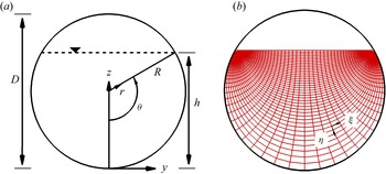
Figure 1(a) presents a cross-section of the flow in a partially filled pipe with the pipe radius  $R$, flow depth in the centre
  $h$ and the water surface width
  $B$. In addition to the Cartesian coordinate system (
 $x,y,z$) in which the Navier–Stokes equations are solved, cylindrical coordinates (
 $x,r,\theta$) (figure 1a) and bipolar coordinates (
 $x,\eta,\xi$) (figure 1b) are used for data analysis. The relationship between the bipolar and the Cartesian coordinate system is (Guo & Meroney Reference Guo and Meroney2013)
 \begin{equation} \frac{y}{R}=\frac{\sin(\theta) \sinh(\xi)}{\cosh(\xi)-\cos(\eta)}, \frac{z-h}{R}=\frac{\sin(\theta) \sin(\eta)}{\cosh(\xi)-\cos(\eta)}, \end{equation}
which transforms the flow domain into a channel where  $\eta ={\rm \pi}$ corresponds to the water surface,
  $\eta ={\rm \pi} +\theta$ to the pipe wall boundary,
  $\xi =0$ to the pipe centreline and
  $\xi =\pm \infty$ to points where the water surface intersects the pipe wall. The advantage of the bipolar system is that it preserves
  $\partial u/ \partial z \propto \partial u/ \partial \eta$ at the water surface and
  $\partial u/ \partial r \propto \partial u/ \partial \eta$ at the pipe wall.

Figure 1. Cross-section of a pipe showing definitions of diameter, radius, water depth, central angle and location of the water surface (a) and bipolar coordinate system in a partially filled pipe flow (b).
The computational set-up of the LES is very similar to the laboratory experiment conducted by Ng et al. (Reference Ng, Cregan, Dodds, Poole and Dennis2018). Table 1 shows the simulated cases and their hydraulic properties, in total four simulations with different water depths,  $h/D = 25\,\%$, 52 %, 75 % and 100 %, are performed. The bulk velocity of
  $U_{b}=0.289$ is maintained for all the cases resulting in bulk Reynolds numbers of
  $Re_{b}\approx 17\,000$–30 000 and Froude numbers of
  $Fr=0.25$–0.69, as given in table 1. The bulk Reynolds number
  $Re_{b}$ is defined as
  $Re_{b}={4R_{h}U_{b}}/{\nu }$ and the Froude number
  $Fr$ is defined as
  $Fr={U_{b}}/{\sqrt {g R_{h}}}$, where
  $R_{h}$ is the hydraulic radius equal to the ratio of flow cross-sectional area and wetted perimeter. Here
  $u_{*}$ is the bulk friction obtained from the mean pressure gradient as
  $u_{*}=\sqrt {{R_{h} \,{\rm d} p/{{\rm d}x}}/{\rho }}$.
Table 1. Hydraulic properties of the four pipe flow simulations.

The length of the pipe is  $L_{x}=22R$ and is considered sufficiently long enough to allow the development of very-large-scale motion (VLSM) as VLSM in a fully filled pipe flow was observed to have a streamwise length scale of
  $\lambda _{x}=8R \thicksim 16R$ (Kim & Adrian Reference Kim and Adrian1999; Guala, Hommema & Adrian Reference Guala, Hommema and Adrian2006; Lee, Sung & Adrian Reference Lee, Sung and Adrian2019). The spanwise and vertical dimensions of the computational domain is set as
  $L_{y}=L_{z}=1.08D$, i.e. slightly larger than the diameter of the pipe, because extra grid points are required for representing the pipe walls using the immersed boundary (IB) method proposed by Uhlmann (Reference Uhlmann2005) and Kara, Stoesser & McSherry (Reference Kara, Stoesser and McSherry2015a). The IB method enforces the no-slip condition at smooth walls and requires a sufficiently fine grid, requiring careful validation. Periodic boundary conditions are applied in the streamwise direction. The location of the water surface is computed in every time step using the LSM which does not require explicit specification of a boundary condition.
Preliminary simulations to validate the method are carried out on different grids to determine the grid size for the production runs (not shown for brevity). The grid consisted of  $1152\times 360\times 360$ grid points, in the
  $x$-,
$x$-,  $y$- and
  $z$-directions, respectively. The grid is uniform in each direction with a grid resolution in wall units of
  ${\rm \Delta} x^{+} \approx 15$,
  ${\rm \Delta} y^{+}_{max} \approx 5$ and
  ${\rm \Delta} z^{+}_{max} \approx 5$. The details of the domains and grids used are summarized in table 2.
Table 2. Domain size and grid resolution of the four LES.

4. Results and discussions
4.1. Validation
Validation of the simulation is an important aspect of any LES serving the purpose of assessing the methods accuracy and the credibility of the main simulations of the study. Therefore, Ng et al. (Reference Ng, Cregan, Dodds, Poole and Dennis2018)'s experiment as well as two recent DNS of fully or partially filled pipe flows, respectively are reproduced using the LES method introduced above. Experimental or DNS data, respectively are then compared with the LES results. Figure 2 presents profiles of the normalised mean streamwise velocity  $u^{+}=\langle \bar {u}\rangle _{x}/u_{*}$ (a), streamwise turbulent fluctuation
  $u^{'+}=\sqrt {\langle \overline {u'u'}\rangle _{x}}/u_{*}$ (b), radial turbulent fluctuation
  $u_{r}^{'+}=\sqrt {\langle \overline {u_{r}'u_{r}'}\rangle _{x}}/u_{*}$ (c) and the wall-normal shear stress
  $u'u_{r}^{'+}=\langle \overline {u'u_{r}'} \rangle _{x}/u_{*}^2$ (d) as a function of the distance from the pipe wall in wall units,
  $r^+=ru_{*}/\nu$, predicted by the LES and DNS of Pirozzoli et al. (Reference Pirozzoli, Romero, Fatica, Verzicco and Orlandi2021) at Reynolds number 17 000 for a fully filled pipe flow (solid lines) and the DNS of Brosda & Manhart (Reference Brosda and Manhart2022) at Reynolds number 15 452 for a semi-filled pipe flow (dashed lines). The
  $\langle \rangle _{x}$ represent the streamwise averaging operator. For a fully filled pipe flow, some discrepancies between the LES and DNS data in the region
  ${\rm d} r^{+}<60$ are observed for the streamwise velocity and the streamwise turbulent fluctuations, however, the LES exhibits good accuracy in this area for a semi-filled pipe flow. The LES does well in predicting the mean velocity profile away from the wall and in matching the peak of the turbulent streamwise fluctuation. The match between LES and DNS is very convincing throughout the domain for the radial turbulent fluctuations and the wall-normal shear stress
  $u_{r}u_{r}^+$, and
  $uu_{r}^+$. It has been observed in Ng et al. (Reference Ng, Cregan, Dodds, Poole and Dennis2018)'s experiments that secondary currents in a partially filled pipe flow influence the flow field and Reynolds stresses near the pipe wall, and, hence, the convincing match between LES and DNS for a semi-filled pipe flow provides confidence in the chosen LES method of this study.

Figure 2. Profiles of the normalised (a) mean streamwise velocity  $u^{+}$, (b) streamwise turbulent fluctuation
  $u^{'+}$, (c) radial turbulent fluctuation
  $u_{r}^{'+}$ and (d) wall-normal shear stress
  $u'u_{r}^{'+}$ as a function of distance from the pipe wall in wall units
  $r^+$, predicted by the LES and the DNS of Pirozzoli et al. (Reference Pirozzoli, Romero, Fatica, Verzicco and Orlandi2021) at Reynolds number 17 000 for a fully filled pipe flow (solid lines) and the DNS of Brosda & Manhart (Reference Brosda and Manhart2022) at Reynolds number 15 452 for a semi-filled pipe flow (dashed lines).
The validation of the LES using the experimental data is similarly successful; figure 3 presents profiles of the streamwise time-averaged velocity (a), the streamwise (b), vertical (c) turbulent intensities and TKE (d) in the centre of a semi-filled pipe as predicted by the LES and as measured in the experiment, data of which is published in Ng et al. (Reference Ng, Cregan, Dodds, Poole and Dennis2018). In general, the LES results agree very well with the experiments, except a slight underestimation of the mean velocity near the water surface and a slight overestimation of the vertical turbulent intensity near the pipe's bottom wall. The so-called ‘velocity dip’ phenomenon, where the location of the maximum streamwise velocity occurs below the free surface, is well predicted by the LES in a partially filled pipe flow in figure 3(a). The normalised streamwise turbulence intensity and TKE profiles, figures 3(b) and 3(d), peak at  $z/h\approx 0.05$, and decrease quickly outside the boundary layer between
  $0.05< z/h<0.1$, and after which it follows a steady linear decrease with depth between
  $0.1< z/h<0.6$. At depth
  $z/h>0.6$, the normalised streamwise turbulence intensity and TKE profiles remain constant until close to the water surface where the values increase suggesting interaction of the flow with the water surface. The vertical turbulence intensity (figure 3c),
  $\langle w^{\prime }_{rms}\rangle _{x}$, peaks a bit further away from the pipe wall than the streamwise component, i.e. at
  $z/h\approx 0.08$, and as expected is attaining zero at the water surface because it is a boundary.

Figure 3. Profiles of the streamwise time-averaged velocity (a), the streamwise (b), vertical (c) turbulent intensities and TKE (d) in the centre of a semi-filled pipe.
Besides the centreline profiles, figure 4 presents contours of the time-averaged streamwise velocity together with secondary current vectors (a,d), the streamwise turbulent intensity (b,e) and the TKE (c,f) in the cross-section of a semi-filled pipe flow as predicted by the LES (a–c) and as measured in the experiment (d–f). The secondary flow in straight partially filled pipes/channels is turbulence driven, i.e. the result of turbulence anisotropy near the water-surface-pipe-wall-corner and is often referred to as Prandtl's secondary flow of the second kind (Prandtl Reference Prandtl1926). The LES reproduces convincingly the velocity, turbulent intensity and TKE distribution.

Figure 4. Contours of the normalised time-averaged streamwise velocity (a,d), streamwise turbulent intensity (b,e) and TKE (c,f) in a semi-filled pipe flow from the LES (a–c) and the experiment (d–f).
Overall, the two LES reproduce very well the flow in fully filled and semi-filled pipe flows and validation of the code's treatment of boundaries as well as the adequacy of spatial and temporal resolution is demonstrated by matching the experimentally observed first- and second-order statistics of these two flows. In the next section the parameter space is expanded in terms of degree of pipe filling and the data are analysed in more detail.
4.2. Mean secondary flow, TKE and turbulence anisotropy
Figure 5 shows the normalised streamwise time-averaged velocity  $u^{+}=\langle \bar {u}\rangle _{x}/u_{*}$ (a), the streamwise normal stress
  $uu^{+}=\langle \overline {u'u'}\rangle _{x}/u_{*}^2$ (b), spanwise normal stress
  $vv^{+}=\langle \overline {v'v'}\rangle _{x}/u_{*}^2$ (c) and vertical normal stress
  $ww^{+}=\langle \overline {w'w'}\rangle _{x}/u_{*}^2$ (d) along the centreline for the four runs as a function of the distance from the pipe wall in wall units. It is observed that in the region
  $z^{+}>10$ the mean streamwise velocity
  $u^{+}$ is higher in half full and three-quarters full pipe flows, while it is lowest in a fully filled pipe flow among the four cases (figure 5a). The ’velocity dip’ is recognized as mean streamwise velocity decreasing near the water surface for half full and three-quarters full flows. Regarding the Reynolds normal stresses, it is firstly noted that all the three components are smallest in quarter full pipe flow (figures 5(b), 5(c), 5(d)), as the Reynolds number in quarter full pipe flow is approximately half of that in the other three cases (table 1). Furthermore, the maximum value of the three Reynolds normal stress components is observed to follow a declining sequence of half full, three-quarters full, fully filled and quarter full (figures 5(b), 5(c), 5(d)). While in the outer region (
 $z^{+}\geqq 30$ in figure 5(b),
  $z^{+}\geqq 100$ in figure 5(c),
  $z^{+}\geqq 210$ in figure 5(d)), the Reynolds normal stresses are highest in fully filled pipe flows. The peak locations for
  $uu^{+}$ are almost constant at approximately
  $z^{+}=16$ for all the four runs. However, the peak locations for
  $vv^{+}$ and
  $ww^{+}$ is smaller in half full and three-quarters full pipe flows compared with a fully filled pipe flow. As shown in figure 4(a), the secondary currents at the pipe centreline go downward toward the pipe wall and are significantly stronger in half full and three-quarters full pipe flows. These downward flows would transport high momentum fluid from the water surface towards the pipe wall, increasing the mean streamwise velocity (figure 5a) and suppressing the turbulent intensities at the outer layer (figures 5(b), 5(c), 5(d)). Subsequently, the boundaries between inner layer and outer layer regions (i.e. the locations where turbulent intensities maximise) are pushed towards the pipe wall.

Figure 5. The normalised streamwise time-averaged velocity  $u^{+}=\bar {u}/u_{*}$ (a), streamwise normal stress
  $uu^{+}=\overline {u'u'}/u_{*}^2$ (b), spanwise normal stress
  $vv^{+}=\overline {v'v'}/u_{*}^2$ (c) and vertical normal stress
  $ww^{+}=\overline {w'w'}/u_{*}^2$ (d) along the centreline for the four runs as a function of the distance from the pipe wall in wall units.
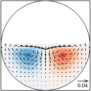
Figure 6 plots contours of time- and streamwise-averaged secondary flow strength normalised with the bulk velocity  $U_{s}/U_{b}$ for (a) quarter full, (b) half full, (c) three-quarters full and (d) fully filled pipe flows. The time-averaged secondary flow strength is calculated as
  $U_{s}=\sqrt {\langle \bar {v}\rangle ^{2}+\langle \bar {w}\rangle ^{2}}$. The time-averaged secondary flow vectors are also plotted in the figures along with reference vectors for the partially filled pipe flows. It can be firstly noted that the secondary flow is strongest in semi-filled and three-quarters filled pipe flows (figures 6(b) and 6(c)). The secondary flow strength attains its maximum at the water surface with magnitudes
  $U_{s}/U_{b}\approx 0.050$ and
  $U_{s}/U_{b}\approx 0.071$ for the semi-filled and three-quarters filled pipe flows, respectively. This is consistent with Ng et al. (Reference Ng, Cregan, Dodds, Poole and Dennis2018) who reported that the secondary flow strength increases by
  $\approx 50\,\%$ with flow depths between
  $h/D=44\,\%$ and
  $h/D=70\,\%$ at a nominally constant Reynolds number (
 $Re\approx 30\,000$). While in quarter filled pipes (figure 6a), the secondary flow strength does not exceed
  $1.5\,\%$ of the bulk velocity and is greatest near the water-surface-pipe-wall-corner, and in fully filled pipe flows it is basically absent. The fact that the secondary currents in a quarter filled pipe are quite weak is probably due to the shallowness of the flow, resulting in rather small (and, hence, weak) secondary flow vortices. All partially filled pipe flows feature a second pair of secondary flow vortices near the wall in the centre of the pipe (figures 6(a), 6(b) and 6(c)) which further reduces the size and strength of the main secondary flow vortex pair in the shallowest case in comparison to the two other partially filled pipe flows. The downward flow from the water surface does not reach the bottom wall, but separates at approximately the half-water depth and reaches the wall near
  $\theta =\pm 1/4 {\rm \pi}$. In the centre of secondary vortices the
  $U_{s}/U_{b}$ is relatively weak for all the four cases.

Figure 6. Contours of time-averaged secondary flow strength normalised with bulk velocity  $U_{s}/U_{b}$ for (a) quarter full; (b) half full; (c) three-quarters full and (d) fully filled pipe flows. The time-averaged secondary flow vector is superimposed for partially filled pipe flows.
In figure 7 contours of the time- and streamwise-averaged streamfunction,  $\phi$ (normalised by the bulk velocity and the pipe radius), is plotted for the four cases investigated. The plots confirm the observations noted above regarding the secondary flow strength and also offer some additional insights. The plots clearly show that the size and location of secondary vortices (high
  $\phi$ magnitude area) differ significantly between the four cases. In half full and three-quarters full pipes, the cross-section is entirely occupied by a pair of counter-rotating streamwise vortices. Their centre, i.e. where
  $\phi$ is maximum, is located near the water surface. This is consistent with what was reported in Ng et al. (Reference Ng, Cregan, Dodds, Poole and Dennis2018). However, in fully filled pipes the magnitude of
  $\phi$ remains negligibly small, indicating nearly absent secondary currents as to be expected. For the quarter full pipe, six weak mean secondary vortices are observed, two symmetric pairs near the centreline, each occupying half-flow depth and the other two near the water-surface-pipe-wall corners. As will be shown latter, secondary currents originate from the water-surface-pipe-wall corners. The size of these secondary currents is limited by the shallow water depth in the quarter full pipe, while it is free to develop in half full and three-quarters full pipes. Consequently, secondary currents near the pipe centreline in quarter full pipe flow are also restricted in the vertical direction. This size limitation from smaller secondary currents is also observed in compound channel flows Kara, Stoesser & Sturm (Reference Kara, Stoesser and Sturm2012), where the depth of the floodplain determines the vertical size of secondary currents in the main channel. The location of the centre of the secondary currents and the magnitude of the streamfunction imply that the secondary currents in partially filled pipes are due to the presence of the (free) water surface causing a (secondary) flow discontinuity. The aspect of origin of the secondary currents is discussed further below.

Figure 7. Contours of the streamfunction normalised with bulk velocity and pipe radius  $U_{b}/R$ for (a) quarter full; (b) half full; (c) three-quarters full and (d) fully filled pipe flows. The time-averaged secondary flow vector is superimposed for the partially filled pipe flows.
Contours of the normalised TKE,  $TKE/u_{*}^2$, are presented in figure 8. In a fully filled pipe the distribution is uniform throughout the pipe and the maximum is observed near the pipe wall. For a partially filled pipe flow, the TKE is non-uniformly distributed due to the geometric asymmetry, is highest near the pipe wall, except for an area in the water-surface-pipe-wall corner where the value of TKE is fairly low. The TKE is produced mainly near pipe walls due to fluid shear. For channel flows, it has been reported that TKE can be produced due to a strongly deformed water surface (McSherry et al. Reference McSherry, Chua, Stoesser and Mulahasan2018); however, in the flows reported here no strong surface deformation occurs due to low
  $Fr$, smooth walls and a completely straight pipe, therefore, the magnitude of TKE near the water surface is relatively small.

Figure 8. Contours of time-averaged TKE normalised with friction velocity for (a) quarter filled; (b) semi-filled; (c) three quarter filled (d) fully filled pipe flows.
Turbulence anisotropy in the four flows is quantified via maps of anisotropy componentality contours. The anisotropy componentality contour map method is proposed by Emory & Iaccarino (Reference Emory and Iaccarino2014), who formulated colours in terms of RGB values by using the coefficients obtained from the eigenvalues of the Reynolds stress anisotropy tensor as
 \begin{equation} \left[\begin{array}{l} R \\ G \\ B \end{array}\right]=C_{1 c}\left[\begin{array}{l} 1 \\ 0 \\ 0 \end{array}\right]+C_{2 c}\left[\begin{array}{l} 0 \\ 1 \\ 0 \end{array}\right]+C_{3 c}\left[\begin{array}{l} 0 \\ 0 \\ 1 \end{array}\right], \end{equation}
where  $C_{1c}, C_{2c}, C_{3c}$ are coefficients defined as
 \begin{equation} \left.\begin{gathered} C_{1c}=\lambda_{1}-\lambda_{2}, \\ C_{2c}=2(\lambda_{2}-\lambda_{3}), \\ C_{3c}=3\lambda_{3}+1, \end{gathered}\right\} \end{equation}
where  $\lambda _{1}$,
  $\lambda _{2}$ and
  $\lambda _{3}$ are the three eigenvalues of the Reynolds stress anisotropy tensor in decreasing order.
In figure 9(e) the original Barycentric map (Banerjee et al. Reference Banerjee, Krahl, Durst and Zenger2007) in which  $C_{1}, C_{2}, C_{3}$, as shown in the insert (figure 9e), indicate the three boundary states of turbulence:
  $C_{1}$ (red colour) describes a flow where turbulent fluctuations only exist along one direction, e.g. rod-like or cigar-shaped turbulence;
  $C_{2}$ (green colour) describes turbulence where fluctuations with equal magnitude exist along two directions; and
  $C_{3}$ (blue colour) represents isotropic turbulence. Figures 9(a) to 9(d) present anisotropy componentality contours for the four cases. For the three partially filled pipe flows, the anisotropy componentality contours show some similarities. First of all, the turbulence along the pipe wall exhibits a distinct
  $C_{1}$ behaviour. This is consistent with the three normal stresses profiles in figure 5, where the streamwise normal stress is significantly higher than the other two components. Another important fact to note is the area of distinct
  $C_{2}$ for the three partially filled pipe flows near the water surface in the centre of the pipe. As shown in figure 5, the presence of the free surface will increase spanwise turbulence near the centre, creating an area where the streamwise and spanwise turbulence dominate the vertical turbulence. This feature is most prominent in the three-quarters full pipe, which also has the strongest mean secondary flow. Some distance below the
  $C_{2}$ area, turbulence returns to isotropic due to larger levels of turbulence intensity in the vertical direction. It has been reported that for flows over smooth walls, the
  $C_{1}$ turbulence occurs very close to the walls (Bomminayuni & Stoesser Reference Bomminayuni and Stoesser2011). Jiménez (Reference Jiménez2013)'s study shows that
  $C_{1}$ turbulence is only observed in the buffer layer or even in the viscous layer near the wall, respectively, while in the log-law region the turbulence is very close to the isotropic state. This is consistent with the results of a fully filled pipe flow, where the turbulence state converges towards isotropic within a small distance away from the pipe wall. In contrast for partially filled pipe flows, the presence of organised secondary currents influences the wall development of turbulence isotropy by suppressing the development of hairpin vortices which will be shown in more detail in § 4.6. Consequently, the one-component turbulence expands to further away from the wall for the partially filled pipe flows (figure 9a–c).

Figure 9. The anisotropy componentality contour maps for (a) quarter filled, (b) semi-filled, (c) three-quarters filled and (d) fully filled pipe flows. (e) Barycentric map.
4.3. Turbulent kinetic energy budget
In this section the budget of the TKE is analysed in light of the origin of secondary currents in pipe flows. The TKE budget is shown as (Nikora & Roy Reference Nikora and Roy2012)
 \begin{equation} \frac{\partial k}{\partial t}+\underbrace{\bar{u}_{j} \frac{\partial k}{\partial x_{j}}}_{{Convection}}={-}\frac{1}{\rho_{o}} \frac{\partial \overline{u_{i}^{\prime} p^{\prime}}}{\partial x_{i}}-\underbrace{\frac{1}{2} \frac{\partial \overline{u_{j}^{\prime} u_{j}^{\prime} u_{i}^{\prime}}}{\partial x_{i}}}_{{Transport}}+\nu \frac{\partial^{2} k}{\partial x_{i}^{2}}-\underbrace{\overline{u_{i}^{\prime} u_{j}^{\prime}} \frac{\partial \overline{u_{i}}}{\partial x_{j}}}_{{Production}}- \underbrace{\nu \frac{\partial u_{i}^{\prime}}{\partial x_{j}} \frac{\partial u_{i}^{\prime}}{\partial x_{j}}}_{{Dissipation}}. \end{equation}
The flow is fully developed so that the rate of change of TKE is zero. Pressure diffusion (the first term on the right-hand side of (4.3)) and molecular viscous transport (the third term on the right-hand side of (4.3)) are usually negligible compared with the other terms in the equations (Nikora & Roy Reference Nikora and Roy2012). Therefore, the four main terms comprising the TKE budget are the TKE convection ( $TKE_{C}$), TKE production (
 $TKE_{P}$), TKE turbulent transport (
 $TKE_{T}$) and TKE dissipation (
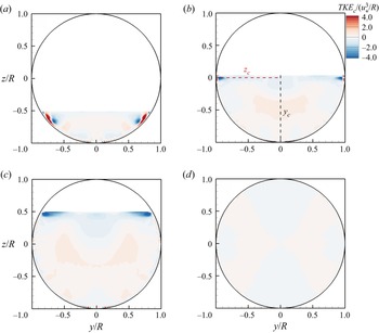
 $TKE_{D}$). Figure 10 shows the contours of convection of TKE by the secondary flow,
  $TKE_{c}$, normalised by
  $(u_{*}^{3}/R)$ for the four cases. For a fully filled pipe flow, the turbulence is isotropic for almost the whole cross-section (figure 9), therefore, no significant
  $TKE_c$ is generated in a fully filled pipe flow (figure 10d). For the quarter full pipe (figure 10a),
  $TKE_{c}$ is observed to be large along the pipe wall and peaks near the water surface. By increasing the water depth to half full and three-quarters full, figures 10(b) and 10(c), the highest magnitude of
  $TKE_{c}$ occurs only in the two corners of pipe wall and water surface, suggesting that secondary currents originate from these locations. In a recent paper, Ng et al. (Reference Ng, Collignon, Poole and Dennis2021) carried out proper orthogonal decomposition of the fluctuating velocity fields showing that low-order mode large-scale cells occupied the pipe-wall-water-surface corners which contributed nearly a quarter to the overall TKE. This is consistent with our findings that an imbalance of the TKE budget (
 $TKE_{c}$) occurs primarily at the water-surface-pipe-wall corners and it drives the secondary motion, in the form of single large-scale streamwise vortices.

Figure 10. Contours of convection of TKE by secondary flow,  $TKE_{c}$, normalised by
  $(u_{*}^{3}/R)$ for (a) quarter filled, (b) semi-filled, (c) three-quarters filled and (d) fully filled pipe flows.
Figure 11 presents contours of the normalised TKE production ,  $TKE_{p}$, and in figure 12 the contours of the TKE dissipation. In a fully filled pipe, both
  $TKE_{p}$ and
  $TKE_{d}$ are distributed uniformly along the pipe wall and their magnitudes are similar, so that these two terms cancel out and, hence, very little turbulent transport occurs. However, for a partially filled pipe flow, near the water surface and the pipe wall, both
  $TKE_{p}$ and
  $TKE_{d}$ are very small, which is due to insignificant TKE shear production and TKE dissipation, which has also been reported by Hsu et al. (Reference Hsu, Grega, Leighton and Wei2000) and Broglia, Pascarelli & Piomelli (Reference Broglia, Pascarelli and Piomelli2003) based on their low aspect ratio open duct flow experiments and simulations. They also reported that far from the wall, the low
  $TKE_{p}$ and
  $TKE_{d}$ would results in an increase of surface-parallel fluctuations very close to the water surface. Consistent with their observations, the LES exhibit higher streamwise and spanwise Reynolds normal stresses at the centreline very close to the water surface (figure 5). This is due to a transfer from the stress normal to the free surface, i.e.
  $w^{\prime }w^{\prime }$, to the streamwise,
  $u^{\prime }u^{\prime }$, and spanwise,
  $v^{\prime }v^{\prime }$, components (Broglia et al. Reference Broglia, Pascarelli and Piomelli2003).

Figure 11. Contours of TKE production,  $TKE_{p}$, normalised by
  $(u_{*}^{3}/R)$ for (a) quarter full, (b) half full, (c) three-quarters full and (d) fully filled pipe flows.

Figure 12. Contours of dissipation of TKE by secondary flow,  $TKE_{d}$, normalised by
  $(u_{*}^{3}/R)$ for (a) quarter filled, (b) semi-filled, (c) three-quarters filled and (d) fully filled pipe flows.
In order to gain a more detailed understanding of the TKE budget at the corner of the pipe wall and water surface, profiles of TKE production  $TKE_{p}$, dissipation
  $TKE_{d}$, turbulent transport
  $TKE_{t}$ and TKE convection
  $TKE_{c}$, all normalised by
  $(u_{*}^{3}/R)$ at
  $y_{c}$ and
  $z_{c}$ (as indicated in figure 10) are plotted in figure 13 for a semi-filled pipe flow. All the terms on the right-hand side of the TKE budget equation have a maximum value near the pipe wall approximately
  $0.03R$ away from the wall. Summing up all the right-hand side terms,
  $TKE_{c}$ along
  $y_{c}$ is almost 0 except near the water surface (
 $r/R=0$), whilst
  $TKE_{c}$ along
  $z_{c}$ reaches a positive peak approximately
  $0.03R$ away from the wall and quickly decreases with increasing distance to the wall. The
  $TKE_{c}$ attains a minimum value at approximately
  $0.07R$ away from the wall and gradually increases to an approximately constant value at
  $r/R=0.8$ higher than the value along
  $y_{c}$.

Figure 13. Profiles of TKE production  $TKE_{p}$, dissipation
  $TKE_{d}$, turbulent transport
  $TKE_{t}$ (a) and TKE convection
  $TKE_{c}$ (b), normalised by
  $(u_{*}^{3}/R)$ for a semi-filled pipe flow at
  $y_{c}$ (black lines) and
  $z_{c}$ (red lines).
4.4. Friction factor decomposition
Firstly the contours of time-averaged boundary normal Reynolds shear stress,  $-\langle \overline {u^{\prime }u_{\eta }^{\prime }\rangle }$ for partially filled pipe flows and
  $-\langle \overline {u^{\prime }u_{r}^{\prime }\rangle }$ for fully filled pipe flows, normalised with friction velocity are shown in figure 14. By referring back to the streamwise velocity distributions in figure 6 we can see that the Reynolds shear stress is minimum where streamwise velocity is maximum. The regions of maximum Reynolds shear stress appear around the periphery of the pipe as expected and not near the free surface which will have much less mean shear than near the no-slip boundary. Interestingly, the regions of high stress (dark shaded regions) do not form a continuous band near the wall, which is the result of the secondary currents transporting fluid away and to the wall, respectively. For all the partially filled flow cases, the regions of maximum stress are where the secondary flow is toward the pipe wall, usually close to bisectors of
  $\theta =({(2n+1)}/{4}){\rm \pi}$. Whereas at locations where the secondary flow is away from the pipe wall, the shear stress is lower. These local near-wall shear stress variations agree with observations in open-channel flows (Nezu & Nakagawa Reference Nezu and Nakagawa1993; Wang & Cheng Reference Wang and Cheng2005), where the shear stress is higher in regions of downward flow and lower in regions of upward flows.

Figure 14. Contours of time-averaged boundary normal Reynolds shear stress normalised with friction velocity for (a) quarter filled, (b) semi-filled, (c) three-quarters filled and (d) fully filled pipe flows. Note that the boundary normal direction for partially filled pipe flows is  ${\partial }/{\partial \eta }$, as shown in figure 1(b), while it is
  ${\partial }/{\partial r}$ for a fully filled pipe flow.
To quantify the effect of viscosity, secondary currents and turbulence on the non-uniform distribution of the wall shear stress shown in figure 14, the friction factor decompostion method proposed by Modesti et al. (Reference Modesti, Pirozzoli, Orlandi and Grasso2018) is applied for the LES results. Modesti et al. (Reference Modesti, Pirozzoli, Orlandi and Grasso2018) derived a generalized version of the FIK identity (Fukagata et al. Reference Fukagata, Iwamoto and Kasagi2002) for duct flows with arbitrary shape, from the mean streamwise momentum balance equation, namely
 \begin{equation} \nu\nabla^2\bar{u}=\boldsymbol{\nabla}\boldsymbol{\cdot} \boldsymbol{\tau}_{\boldsymbol{C}}+ \boldsymbol{\nabla}\boldsymbol{\cdot}\boldsymbol{\tau}_{\boldsymbol{T}}-\bar{\varPi}, \end{equation}
where  $\bar {u}$ is the mean streamwise velocity,
  $\boldsymbol {\tau }_{\boldsymbol {C}}=\bar {u}\overline {\boldsymbol {u}_{\boldsymbol {yz}}}$ is associated with mean cross-stream convection,
  $\boldsymbol {\tau }_{\boldsymbol {T}}=\overline {u' \boldsymbol {u}'_{\boldsymbol {yz}}}$ is associated with turbulence convection,
  $\boldsymbol {u}_{\boldsymbol {yz}}=(v,w)$ is the cross-stream velocity vector and
  $\bar {\varPi }=u_{*}^2/R_{h}$ is the driving pressure gradient. Equation (4.4) may be interpreted as a Poisson equation for the mean streamwise velocity, with the right-hand side source terms obtained from the LES. Hence, the solution of (4.4) may be cast as the superposition of three parts, namely
  $\bar {u}=\overline {u_{V}}+\overline {u_{T}}+\overline {u_{C}}$, with
 \begin{gather} \nu\nabla^2\overline{u_{V}}={-}\bar{\varPi}, \end{gather}
 \begin{gather}\nu\nabla^2\overline{u_{T}}=\boldsymbol{\nabla} \boldsymbol{\cdot} \boldsymbol{\tau}_{\boldsymbol{T}}, \end{gather}
 \begin{gather}\nu\nabla^2\overline{u_{C}}=\boldsymbol{\nabla} \boldsymbol{\cdot} \boldsymbol{\tau}_{\boldsymbol{C}}, \end{gather}
where  $\overline {u_{V}}$,
  $\overline {u_{T}}$ and
  $\overline {u_{C}}$ denote the viscous, turbulent and secondary currents’ contributions to the mean streamwise velocity field. The bulk velocity can accordingly be evaluated as
 \begin{equation} u_{b}=u_{bV}+u_{bT}+u_{bC},\quad u_{bX}=1/A \int_{A} \overline{u_{X}}\,{\rm d} A, \end{equation}
where  $A$ represents the cross-section area. Inserting the Darcy–Weisbach friction factor
  $f=8u_{*}^2/u_{b}^2$ into (4.8a,b), we obtain
 \begin{equation} f=\frac{8u_{*}^2}{u_{bV}u_{b}}\left(1-\frac{u_{bT}}{u_{b}}-\frac{u_{bC}}{u_{b}} \right)=f_{V}+f_{T}+f_{C}. \end{equation}
Equation (4.9) shows that the Darcy–Weisbach friction factor,  $f$, in pipe flows can be decomposed into three components: the viscous contribution, the turbulent contribution due to small-scale turbulence and the convection contribution due to secondary currents. Figures 15, 16 and 17 plot the normalised viscous, turbulent and secondary currents’ contribution to the mean streamwise velocity as defined in (4.5), (4.6) and (4.7) for the four cases. The viscous-associated velocity field
  $u_{V}$, shown in figure 15, arises from the solution of a Poisson equation with a uniform right-hand side (the pressure gradient); hence, its geometry is identical to the case of Stokes flow depending only on the cross-sectional geometry. The turbulence-associated velocity field
  $u_{T}$, shown in figure 16, is everywhere negative highlighting a retarding effect of turbulence on the bulk flow. For a quarter filled pipe flow and fully filled pipe flow, the turbulence-associated velocity field is topologically similar to the viscous-associated field, while for semi-filled and three-quarters filled pipe flows, the magnitude of
  $u_{T}$ is lower near the water surface at the pipe centreline. The velocity field
  $u_{C}$ induced by the secondary currents, shown in figure 17, has a more complex organisation. The contribution of secondary currents is significantly higher in semi-filled and three-quarters filled pipe flows due to a much stronger secondary flow strength, as shown in figure 6. Moreover, the
  $u_{C}$ reverses sign at locations
  $z/R\approx -0.5$, indicating an accelerating effect of secondary currents on the streamwise flow, consistent with the results in figure 5(a).

Figure 15. Normalised viscous contribution to the mean streamwise velocity,  $u_{V}/u_{b}$, for (a) quarter filled, (b) semi-filled, (c) three-quarters filled and (d) fully filled pipe flows.

Figure 16. normalised turbulent contribution to the mean streamwise velocity,  $u_{T}/u_{b}$, for (a) quarter filled; (b) semi-filled; (c) three-quarters filled (d) fully filled pipe flows.

Figure 17. Normalised secondary currents’ contribution to the mean streamwise velocity,  $u_{C}/u_{b}$, for (a) quarter filled, (b) semi-filled, (c) three-quarters filled and (d) fully filled pipe flows. The dashed lines shown in partially filled pipe flows are
  $u_{C}/u_{b}=0$.
The friction factor of the four cases is calculated from (4.9) and the contributions of the three stress constituents (viscous, turbulent and secondary currents) are quantified in figure 18. It is first observed that the viscous contribution decreases at higher flow depths, due to higher bulk Reynolds numbers. The secondary currents’ contribution is high in semi-filled and three-quarters filled pipe flows with up to 10 % while it is relatively small in the other two cases. It is particularly interesting that the friction factor,  $f$, in semi-filled and three-quarters filled pipe flows is lower than the other two cases. These friction factors are compared with those obtained from the Kármán–Prandtl resistance equation at the same bulk Reynolds numbers in table 3. It can be seen that the friction factors in semi-filled and three-quarters filled pipe flows are 5.6 % and 2.47 % less than the Kármán–Prandtl resistance equation, respectively, whereas in quarter filled and fully filled pipe flows they are 0.22 % and 1.14 % higher. This phenomenon is contrary to the common understanding that secondary currents increase the bulk friction factor compared with the case when secondary currents are absent (Nikora & Roy Reference Nikora and Roy2012). However, there are also indications that in some situations secondary flows do not affect the bulk friction factor (Kean et al. Reference Kean, Kuhnle, Smith, Alonso and Langendoen2009), or even reduces the friction factor in duct flows (Modesti et al. Reference Modesti, Pirozzoli, Orlandi and Grasso2018) and in open-channel flows (Zampiron, Cameron & Nikora Reference Zampiron, Cameron and Nikora2020). A recent investigation by Yao, Chen & Hussain (Reference Yao, Chen and Hussain2018) has shed light on the mechanisms of how secondary currents influence the bulk friction factor. They performed DNS in channel flow with artificial spanwise opposed wall-jet currents added near the channel bottom wall, and demonstrated that the presence of these artificial secondary currents reduces drag by merging low-speed streaks and reducing streak strength below the critical values required for streak instability as well as for transient growth. Consequently, the generation of drag inducing near-wall streamwise vortices is suppressed. In this study, though the secondary currents are not artificially added to the pipes but driven by the anisotropy of the Reynolds stress, the effects on low-speed streaks and near-wall streamwise vortices are also observed here (and will be shown in § 4.6). In terms of the friction factor decomposition, the presence of secondary currents causes a significant decrease of the turbulent stress contribution as well as a decrease of the total friction factor (Yao et al. Reference Yao, Chen and Hussain2018), as shown in figure 18.

Figure 18. Contributions of viscous (Vis), turbulent (Turb) and secondary currents induced (Sc) friction factor to the friction factor for quarter filled (a), semi-filled (b), three-quarters filled (c) and fully filled pipe flows (d).
Table 3. Comparison between friction factors from the LES and from Kármán–Prandtl resistance equation at the same bulk Reynolds numbers.

4.5. Pre-multiplied spectra
In order to study the influence of secondary currents on coherent structures, pre-multiplied spectra of the streamwise velocity component,  $k\varPhi _{uu}/u_{*}^{2}$, at various locations along the centreline are plotted in figure 19 for the four cases. For a fully filled pipe flow (figure 19d), there are two peaks in the pre-multiplied spectra visible at locations
  $z= 0.3R$ and
  $z= 0.1R$. The peak at the lower wavenumber marked with an arrow in figure 19(d) has been reported for fully filled pipe flows and has been recognized as the VLSM in both pipe and channel flows (Kim & Adrian Reference Kim and Adrian1999; Guala et al. Reference Guala, Hommema and Adrian2006; Lee et al. Reference Lee, Sung and Adrian2019). The fully filled pipe simulation successfully captures the VLSM. For partially filled pipe flows (figure 19a–c), no significant second peak at a low wavenumber range is observed, suggesting an absence of VLSM for these flows. In addition, pre-multiplied spectra of the streamwise velocity component at different azimuthal locations at constant wall distance
  $z=0.1R$ for a partially filled pipe flow are presented in figure 20. All spectra peak at relatively high wavenumber
  $kR\geqq 3$ confirming the absence of VLSM in the entire cross-section. The magnitude of the energy at higher azimuthal angles (figure 20c,d) is slightly less than that at lower azimuthal angles (figure 20a,b), suggesting reduced streamwise velocity fluctuations near the water surface. Yao et al. (Reference Yao, Chen and Hussain2018) show that the energy containing motion in channel flows is significantly suppressed due to imposed secondary currents, suggesting that the absence of VLSM in partially filled pipe flows is caused by the presence of the secondary currents. The absence of VLSMs from figures 19 and 20 is consistent with the observation in Ng et al. (Reference Ng, Cregan, Dodds, Poole and Dennis2018)'s experiments. Recently, Ng et al. (Reference Ng, Collignon, Poole and Dennis2021) show that there are more large-scale motions and VLSMs in partially filled pipe flows with
  $h/D=80\,\%$ than with
  $h/D=44\,\%$ and
  $h/D=62\,\%$. For structure lengths
  $8\leq \delta T U_b/R_h\leq 13$, there are an appreciably greater number of events for
  $h/D=80\,\%$. Further, contour maps of pre-multiplied spectra of the streamwise velocity component
  $k\varPhi _{uu}/u_{*}^{2}$ in the pipe centre plane for semi-filled (a) and fully filled pipe flows (b) are presented in figure 21. In both semi-filled and fully filled pipe flows a high energy containing motion with wavelength
  $\lambda _{x}/R \leqq 3$ is found near the pipe walls. These motions presumably correspond to quasi-streamwise vortices as shown by Yao et al. (Reference Yao, Chen and Hussain2018). With increasing distance from the pipe wall, the peak of the wavelength
  $\lambda _{x}/R$ slightly increases. Besides the low-wavelength motion, VLSM is found for fully filled pipe flows with wavelength
  $8\geqq \lambda _{x}/R \leqq 11$ at location
  $z/R\leqq -0.8$, which is similar to other findings of VLSM in turbulent pipe flows, e.g.
  $12\geqq \lambda _{x}/R \leqq 14$ (Kim & Adrian Reference Kim and Adrian1999) and
  $8\geqq \lambda _{x}/R \leqq 16$ (Guala et al. Reference Guala, Hommema and Adrian2006).

Figure 19. Pre-multiplied spectra of the streamwise velocity component  $k\varPhi _{uu}/u_{*}^{2}$ at various vertical locations along the centreline for quarter filled (a), semi-filled (b), three-quarters filled (c) and fully filled pipe flows (d).

Figure 20. Pre-multiplied spectra of the streamwise velocity component  $k\varPhi _{uu}/u_{*}^{2}$ at various azimuthal locations, (a)
  $\theta =1/8{\rm \pi}$, (b)
  $\theta =1/4{\rm \pi}$, (c)
  $\theta =3/8{\rm \pi}$ and (d)
  $\theta =1/2{\rm \pi}$ at constant wall distance
  $z=0.1R$ for the partially filled pipe flows.

Figure 21. Contour maps of pre-multiplied spectra of the streamwise velocity component  $k\varPhi _{uu}/u_{*}^{2}$ in the pipe centre for semi-filled (a) and fully filled pipe flows (b).
Contour maps of pre-multiplied co-spectra of the streamwise and vertical velocity component  $k\varPhi _{uw}/u_{*}^{2}$ in the pipe centre for semi-filled (a) and fully filled pipe flows (b) is shown in figure 22. The most significant difference between the semi-filled and fully filled pipe flows is the shape of the area of high
  $k\varPhi _{uw}/u_{*}^{2}$. For a fully filled pipe, the highest
  $k\varPhi _{uw}/u_{*}^{2}$ is found at small wavelength
  $\lambda _{x}/R$, while for a semi-filled pipe, the pre-multiplied co-spectra with wavelength
  $1\geqq \lambda _{x}/R \leqq 3$ contributes most to the total shear stresses. This is consistent with the findings in figure 14 that the turbulent contribution (i.e. contribution from small-scale turbulence) accounts for the majority of total shear stress in a fully filled pipe while the secondary-current-induced stress, of a larger length scale, has a higher contribution in semi-filled pipe flows. In a fully filled pipe flow the area of high
  $k\varPhi _{uw}/u_{*}^{2}$ extends vertically away from the wall with length scales increasing. This is intensively observed by experiments and numerical simulations and has been shown to be the results of wall-generated hairpin packets (Hutchins & Marusic Reference Hutchins and Marusic2007; Jiménez Reference Jiménez2018). Interestingly, in a semi-filled pipe flow the region of highest
  $k\varPhi _{uw}/u_{*}^{2}$ is restricted to very close to the pipe wall. As shown by the mean secondary flow vectors in figure 6, there is a strong downward flow at the centreline in a semi-filled pipe flow. This vertical fluid motion restricts the development of near bed coherent structures, especially their vertically transport, consequently resulting in a confined region of high
  $k\varPhi _{uw}/u_{*}^{2}$.

Figure 22. Contour maps of pre-multiplied co-spectra of the streamwise and vertical velocity components  $k\varPhi _{uw}/u_{*}^{2}$ in the centre of the pipe for semi-filled (a) and fully filled pipe flows (b).
4.6. Two-point correlations and streaks
With the goal to establish the characteristics of the time-average flow structure, spatial-temporal two-point correlations of streamwise velocity fluctuations are calculated using (4.10), where the zero subscripts denote the fix-point of the correlation,
 \begin{equation} R_{uu}({\rm \Delta} x, {\rm \Delta} y, {\rm \Delta} z)= \frac{\overline{u(x_{0}+{\rm \Delta} x,y_{0}+{\rm \Delta} y,z_{0}+{\rm \Delta} z)u(x_{0},y_{0},z_{0})}}{u_{rms}^{2}} \end{equation}
Figure 23 presents two-dimensional two-point correlations of the streamwise velocity computed along the centreline at  $z/R=-0.9$ (a),
  $-$0.7 (b),
  $-$0.5 (c) and
  $-$0.2 (d). Here solid lines represent
  $R_{uu}=0.2$ and dashed lines
  $R_{uu}=-0.2$. The black line represents a fully filled pipe flow and the red line represents a semi-filled pipe flow. The blue dots indicate the location of the fix point of the correlation. In general, the two-dimensional two-point correlation plots agree very well with the results from Ng et al. (Reference Ng, Cregan, Dodds, Poole and Dennis2018). For all four locations, the positively correlated regions are smaller for semi-filled pipe flows compared with those in fully filled pipe flows suggesting a reduction in the size of turbulence structures. Regions of negative correlation are observed when the correlation fix point is at
  $z/R=-0.9$ for fully filled pipe flows only and at correlation centre
  $z/R=-0.7$ for both flows. However, the negatively correlated regions at correlation centre
  $z/R=-0.7$ for a semi-filled pipe is almost invisible in figure 23(b).

Figure 23. Contours of the cross-section  $R_{uu}$ map for fully (black) and semi-filled (red) pipe flows. Correlations are calculated along the centreline at
  $z/R=-0.9$ (a),
  $-$0.7 (b),
  $-$0.5 (c) and
  $-$0.2 (d). Solid lines represent
  $R_{uu}=0.2$ and dashed lines represent
  $R_{uu}=-0.2$.
The contour lines of  $R_{uu}$ reveal that the width and spacing of near-wall streaks in semi-filled pipe flows is influenced by the secondary currents, especially near the pipe wall. Figure 24 presents snapshots of instantaneous streamwise velocity fluctuation at various radii for fully filled pipe flows and figure 25 presents the analogue for semi-filled pipe flows. In figures 24 and 25,
  $s/R$ represents the distance along the angular direction. In figure 24(a) the presence of very long, streamwise-aligned streaky structures characterised by streamwise velocity fluctuations alternating from positive to negative and with lengths O(8R) is observed. As shown in figure 21, these features are the signature of VLSM identified in § 4.5 and which have also been reported in both pipes and channels from experimental and numerical investigations; see, e.g. Guala et al. (Reference Guala, Hommema and Adrian2006), Hutchins & Marusic (Reference Hutchins and Marusic2007) and Cameron, Nikora & Stewart (Reference Cameron, Nikora and Stewart2017). The elongated streaks are still visible a bit away from the wall (figure 24b), however disappear with distance from the wall (figure 24c,d). In terms of a semi-filled pipe flow, a prominent difference is observed for the streaks at
  $r/R=-0.9$ in figure 25(a). Both the width and the spacing of the streaks are shorter in comparison to fully filled pipe flow streaks, and are limited to a streamwise length of
  $\lambda \leq 5R$. With increasing the distance from the wall, the streamwise-aligned streaky structures gradually vanish and the snapshot of streamwise velocity fluctuation at
  $r/R=-0.2$ (figure 25d) looks similar to that in a fully filled pipe flow (figure 24d). Figure 25 supports these findings in § 4.4 that the near bed streaks are suppressed by the presence of secondary currents. Figure 26 presents isosurfaces of the
  $Q$-criterion of
  $Q=300$ for fully filled (a) and semi-filled (b) pipe flows. The
  $Q$ iso-surface, as first proposed by Hunt, Wray & Moin (Reference Hunt, Wray and Moin1988), is contoured with distance from the pipe centre. Figure 26 visualises a dramatic decrease in the number of coherent structures in semi-filled pipe flows, especially near the pipe centreline at
  $y/R=0$ where the secondary flow transports high momentum fluid towards the pipe wall. The absence of coherent structures near the pipe centreline for partially filled flow is also confirmed by Ng et al. (Reference Ng, Collignon, Poole and Dennis2021), who show that large-scale cells populate the corners where the pipe wall meets the water surface. Moreover, the coherent structures in semi-filled pipe flows are more aligned in the streamwise direction and almost of constant length while those in fully filled pipe flows vary in size and are not necessarily aligned with the streamwise direction (particularly near the wall, i.e. red structures), suggesting more meandering of the flow in fully filled pipe flows. This underlines the findings from figure 9, i.e. that the turbulence structure in semi-filled pipe flows is prominently one dimensional near the wall, whereas in fully filled pipe flows it tends to be two dimensional near the walls and isotropic towards the centre. Furthermore, a proportion of the coherent structures in fully filled pipe flows transport away from the wall at
  $r/R>0.9$, while very few coherent structures in semi-filled pipe flows reach these locations.

Figure 24. Contours of instantaneous streamwise velocity fluctuations for a fully filled pipe flow at radius  $r/R=-0.9$ (a),
  $-$0.7 (b),
  $-$0.5 (c) and
  $-$0.2 (d).

Figure 25. Contours of instantaneous streamwise velocity fluctuations for a semi-filled pipe flow at radius  $r/R=-0.9$ (a),
  $-$0.7 (b),
  $-$0.5 (c) and
  $-$0.2 (d).

Figure 26. Isosurface of  $Q=300$ for a (a) fully filled pipe flow and (b) semi-filled pipe flow. The Isosurface is contoured with distance from the pipe centre,
  $r/R$, and the plots are from the top view. The structures at the top half-part, i.e.
  $z/R>0$, are blanked to make the plots clearer.
5. Conclusions
Large-eddy simulations of turbulent flow in fully and partially filled pipes were performed. The simulations were validated first using DNS and experimental data. Large-eddy simulations predicted centreline profiles of the time-averaged streamwise velocity, normal stresses and TKE were found to be in convincing agreement with DNS or experimental data, respectively. The presence of time-averaged secondary flows was observed by examination of the secondary velocity vectors and the streamfunction. The secondary flow is stronger for semi-filled and three-quarters filled pipe flows in comparison to quarter filled pipes, whilst it is absent in a fully filled pipe flow. Moreover, the strong secondary flows occupy the entire cross-section forming a pair of symmetric vortices in semi-filled and three-quarters filled pipes, while for quarter full pipes more than two pairs of weak vortices are formed. There is no time-averaged secondary flow in fully filled pipe flows. The turbulence anisotropy in partially and fully filled pipes has been visualised by the anisotropy componentality contours map method (Emory & Iaccarino Reference Emory and Iaccarino2014). Compared with mainly isotropic turbulence in fully filled pipe flows (except very close to the wall), a thick layer of one-component turbulence is formed along the wall in partially filled pipe flows. Furthermore, an area of two-component turbulence is present at the water surface near the centreline bisector. The origin of the mean secondary flow was examined with the TKE budget, which suggested that secondary currents originate from the corner between the water surface and the pipe walls. Production of TKE and streamwise vorticity at this corner is larger than the sum of turbulent transport and dissipation, which results in a mean convection of TKE and streamwise vorticity by secondary flows. Different from the TKE budget, an extra source of streamwise vorticity production is found at the free surface near the centreline bisector, which is thought to be caused by the two-component asymmetric turbulence at this location. Despite the fact that strong secondary currents (in semi-filled and three-quarters filled pipes) yield a dispersive shear stress which contributes to the friction factor, the turbulent shear stress contribution to the friction factor is reduced disproportionately, which results in a reduction of the total friction factor in comparison to fully or quarter filled pipe flows. The influence of secondary currents on coherent structures is further investigated by presenting pre-multiplied spectra, two-point correlation functions as well as instantaneous streaks and vortices (visualised with the Q-criterion). It has been found that the presence of secondary currents prevents the formation of VLSMs, due to the secondary flow disrupting the formation and growth of organised near-wall streaks. The near-wall two-component turbulence is nearly absent (presence of elongated streamwise-aligned structures) in semi-filled and three-quarters filled pipes resulting in less turbulent shear near the walls and which proved to be responsible for the drag reduction in partially filled pipe flows.
Acknowledgements
The authors would like to acknowledge the support of the high performance computing centers of the University College London and of Tsinghua University.
Funding
Financial support for this work is provided by the EPSRC/UK project ‘Distributed Fibre-optic Cable Sensing for Buried Pipe Infrastructure’, EP/S016376/1.
Declaration of interests
The authors report no conflict of interest.