


1. Introduction
Particle-laden turbulent flows are ubiquitous in both natural phenomena and industrial applications. Examples include rain formation (Shaw Reference Shaw2003; Grabowski & Wang Reference Grabowski and Wang2013), dust devils (Balme & Greeley Reference Balme and Greeley2006), pollutant control (Jaworek et al. Reference Jaworek, Marchewicz, Sobczyk, Krupa and Czech2018) and industrial sprays (Shrimpton & Yule Reference Shrimpton and Yule1999; Tryggvason, Scardovelli & Zaleski Reference Tryggvason, Scardovelli and Zaleski2011). As a result of the strong turbulent fluctuation, suspended particles often experience frequent collisions, which directly lead to droplet coalescence (Onishi, Matsuda & Takahashi Reference Onishi, Matsuda and Takahashi2015; Bec et al. Reference Bec, Ray, Saw and Homann2016), agglomerate formation (Chen, Li & Marshall Reference Chen, Li and Marshall2019a) and charge transfer (Jin & Marshall Reference Jin and Marshall2017). Due to its importance and complexity, the issue of the turbulence-enhanced collision has attracted widespread attention.
The pioneering work by Saffman & Turner (Reference Saffman and Turner1956) first revealed the essential role of turbulent collision in rain formation and formulated the collision kernel of non-inertial droplets. Then, by introducing the radial distribution function (RDF) and the relative velocity distribution, the collision kernel of inertial particles in dilute systems is expressed as (Sundaram & Collins Reference Sundaram and Collins1997; Wang, Wexler & Zhou Reference Wang, Wexler and Zhou2000)
 \begin{equation}\varGamma = 2{\rm \pi} R_c^2 \cdot g({R_c}) \cdot \langle |{w_r}|\rangle .\end{equation}
Here,  ${R_c}$ is the collision distance,
  $g({R_c})$ is the RDF at contact and
  ${w_r}$ is the radial relative velocity. The effects of turbulence on particle collisions can then be quantified by the spatial dispersion and the radial relative velocity.
The turbulent dispersion of inertial particles has been extensively investigated. Due to the centrifugal effect, inertial particles were found to cluster in regions with low vorticity and high strain rate, which is known as preferential concentration (Maxey Reference Maxey1987; Squires & Eaton Reference Squire and Eaton1991; Eaton & Fessler Reference Eaton and Fessler1994). Different mathematical descriptions have been employed to characterize this phenomenon, and the maximum clustering is generally observed when particle's Stokes number is around unity (Squires & Eaton Reference Squire and Eaton1991; Wang et al. Reference Wang, Wexler and Zhou2000; Balkovsky, Falkovich & Fouxon Reference Balkovsky, Falkovich and Fouxon2001; Bec et al. Reference Bec, Biferale, Cencini, Lanotte, Musacchio and Toschi2007; Calzavarini et al. Reference Calzavarini, Kerscher, Lohse and Toschi2008a,Reference Calzavarini, Cencini, Lohse and Toschib; Goto & Vassolicos Reference Goto and Vassilicos2008; Monchaux, Bourgoin & Cartellier Reference Monchaux, Bourgoin and Cartellier2010; Tagawa et al. Reference Tagawa, Mercado, Prakash, Calzavarini, Sun and Lohse2012). Preferential concentration could significantly enrich the local particle concentration and thus enhance interparticle collisions (Reade & Collins Reference Reade and Collins2000; Marchioli & Soldati Reference Marchioli and Soldati2002; Chun et al. Reference Chun, Koch, Rani, Ahluwalia and Collins2005; Salazar et al. Reference Salazar, de Jong, Cao, Woodward, Meng and Collins2008; Saw et al. Reference Saw, Shaw, Ayyalasomayajula, Chuang and Gylfason2008; Jayaram et al. Reference Jayaram, Jie, Zhao and Andersson2020). More details about particle dispersion can be found in several reviews and the references therein (Falkovich, Gawedzki & Vergassola Reference Falkovich, Gawedzki and Vergassola2001; Balachandar & Eaton Reference Balachandar and Eaton2009; Toschi & Bodenschatz Reference Toschi and Bodenschatz2009; Mathai, Lohse & Sun Reference Mathai, Lohse and Sun2020). With regard to the radial relative velocity, both numerical simulations (Gustavsson & Mehlig Reference Gustavsson and Mehlig2014; Ireland, Bragg & Collins Reference Ireland, Bragg and Collins2016a,Reference Ireland, Bragg and Collinsb; James & Ray Reference James and Ray2017; Bhatnagar et al. Reference Bhatnagar, Gustavsson, Mehlig and Mitra2018a; Bhatnagar, Gustavsson & Mitra Reference Bhatnagar, Gustavsson and Mitra2018b) and experimental studies (de Jong et al. Reference de Jong, Salazar, Woodward, Collins and Meng2010; Saw et al. Reference Saw, Bewley, Bodenschatz, Ray and Bec2014; Dou et al. Reference Dou, Bragg, Hammond, Liang, Collins and Meng2018) have been conducted to systematically investigate the relative velocity statistics. The impacts of particle inertia and Taylor Reynolds number are further elaborated.
When particle inertia continues to increase, the sling effect or the formation of caustics can be initiated by intermittent turbulent fluctuations (Falkovich, Fouxon & Stepanov Reference Falkovich, Fouxon and Stepanov2002; Wilkinson & Mehlig Reference Wilkinson and Mehlig2005; Wilkinson, Mehlig & Bezuglyy Reference Wilkinson, Mehlig and Bezuglyy2006). During a sling process, the particle velocity gradient detaches from the local flow field and diverges within a finite time. As a result, the particle velocity field becomes multivalued at certain positions, where particles could collide with each other at a large relative velocity (Bewley, Saw & Bodenschatz Reference Bewley, Saw and Bodenschartz2013). This eventually leads to a surge in collision frequency (Falkovich & Pumir Reference Falkocivh and Pumir2007; Voßkuhle et al. Reference Voßkuhle, Pumir, Lévêque and Wilkinson2014).
Recently, by correlating collision events with local flow characteristics, the essential role of flow structures (e.g. straining zones and intense vortical structures) in the agglomeration and deagglomeration process is unveiled. It is reported that the straining zones contribute predominantly to head-on collisions, while intense vortices could rapidly eject particles and cause violent collisions (Perrin & Jonker Reference Perrin and Jonker2014, Reference Perrin and Jonker2016; Agasthya et al. Reference Agasthya, Picardo, Ravichandran, Govindarajan and Ray2019; Picardo et al. Reference Picardo, Agasthya, Govindarajan and Ray2019; Chen & Li Reference Chen and Li2020).
In addition to the ideal non-interacting particles, actual particles often interact with each other through complex interactions, such as the pure elastic force (Bec, Musacchio & Ray Reference Bec, Musacchio and Ray2013), the short-range soft repulsion (Gupta et al. Reference Gupta, Chaudhuri, Bec and Ray2018), van der Waals adhesion (Breuer & Almohammed Reference Breuer and Almohammed2015; Almohammed & Breuer Reference Almohammed and Breuer2016; Chen et al. Reference Chen, Li and Marshall2019a) and electrostatic interactions (Lee et al. Reference Lee, Waitukaitis, Miskin and Jaeger2015). The electrostatic interactions are of interest in the present study. Particles suspended in turbulent flows usually carry electrical charge through triboelectrification or the sticking of free ions to the surface (Jones Reference Jones1995; McCarty & Whitesides Reference McCarty and Whitesides2008; Pähtz, Herr,amm & Shinbrot Reference Pähtz, Herr,amm and Shinbrot2010; Kolehmainen et al. Reference Kolehmainen, Ozzel, Gu, Shinbrot and Sundaresan2018). Such systems can be found in the particle-laden flue gas in electrostatic precipitators (Jaworek et al. Reference Jaworek, Marchewicz, Sobczyk, Krupa and Czech2018), the sandstorms and dust devils on Earth or Mars (Di Renzo & Urzay Reference Di Renzo and Urzay2018; Zhang & Zhou Reference Zhang and Zhou2020) and the plumes after volcanic eruptions (Gilbert et al. Reference Gilbert, Lane, Sparks and Koyaguchi1991). Compared with the neutral case, the long-range electrostatic force could significantly modify the particle dynamics. For instance, the clustering of like/opposite-charged particles will be inhibited/enhanced (Karnik & Shrimpton Reference Karnik and Shrimpton2012; Yao & Capecelatro Reference Yao and Capecelatro2018; Boutsikakis et al. Reference Boutsikakis, Fede, Pedrono and Simonin2020), and mesoscale electrical fields can be generated by the spatial separation of electrical charge (Di Renzo & Urzay Reference Di Renzo and Urzay2018). By including the Coulomb force into the Fokker–Planck equation, Lu et al. (Reference Lu, Nordsiek, Saw and Shaw2010) successfully predicted the RDF for like-charged particles with finite inertia. Furthermore, for particles with negligible inertia and weak charge, by assuming that the velocities induced by turbulence and the Coulomb force could be superposed, a general model was proposed to predict charged particle behaviour in turbulence (Lu & Shaw Reference Lu and Shaw2015). But for larger particle inertia  $(\text{Stokes number } St \ge 1)$, although several studies have reported the dynamics of charged particles in turbulence, the understanding is still very limited. We thus focus on the dynamics of charged particles with
  $St \ge 1$.
Regarding the turbulent agglomeration of identically charged particles, however, few studies have been done on the collision frequency. Besides, the influences of particle charge on the subsequent collision and adhesion processes are less understood. In order to describe these processes, a comprehensive model is required to calculate the contact forces and torques between colliding particles. More recently, by using a direct numerical simulation (DNS)-discrete element method (DEM) coupled approach, Chen et al. (Reference Chen, Li and Marshall2019a) and Chen & Li (Reference Chen and Li2020) investigated the agglomeration and deagglomeration of neutral particles in homogeneous isotropic turbulence and showed that the particle-scale contact interactions significantly affected the agglomeration/deagglomeration rates. However, it is still not clear how the presence of the electrostatic force will change this physical picture.
In this study, we try to address the above issues by numerically investigating the agglomeration of charged particles in turbulence. DNS is adopted to evolve the homogeneous isotropic turbulence, and the adhesive DEM is implemented to calculate particle motions. In particular, the long-range Coulomb force is calculated using the fast multipole method (FMM). The impact of Coulomb repulsion on the collision frequency between charged particles is quantified in terms of the equilibrium collision kernel. By using a decomposition analysis, we are able to identify the contributions from preferential concentration and the sling effect to the collision kernel. The modified adhesion parameter,  $A{d_n}$, defined as the ratio of interparticle adhesion to particle inertia, is then introduced to predict the post-collision behaviour. By comparing the number of sticking events, the combined effect of the Coulomb force and interparticle adhesion is elucidated. In the end, the agglomerate structure, which is described by the fractal dimension, is examined for both neutral and charged particles.
2. Methods
In this section, we introduce the numerical methods of the Eulerian--Lagrangian-based simulation. The fluid phase is evolved using DNS (§ 2.1), and the motions of suspended solid particles are computed by DEM (§ 2.2). Since various time scales are involved in the present simulation, the multiple time step algorithm is adopted to accelerate the calculation (§ 2.3). The dimensionless parameters and simulation conditions are then discussed in § 2.4.
2.1. Gas phase: DNS
The DNS of incompressible homogeneous and isotropic turbulence is performed using a pseudo-spectral method. The computational domain is a triply periodic cubic box with a side length  $L = 2{\rm \pi}$. The Cartesian grid number
  ${N^3}$ equals
  ${128^3}$. The governing equations of the fluid phase are given by
 \begin{equation}\boldsymbol{\nabla }\boldsymbol{\cdot }\boldsymbol{u} = 0,\end{equation}
and
 \begin{equation}\frac{{\partial \boldsymbol{u}}}{{\partial t}} + \boldsymbol{u}\boldsymbol{\cdot }\boldsymbol{\nabla }\boldsymbol{u} ={-} \frac{1}{{{\rho _f}}}\boldsymbol{\nabla }p + \nu {\nabla ^2}\boldsymbol{u} + {\boldsymbol{f}_F} + {\boldsymbol{f}_P},\end{equation}
where  $\boldsymbol{u}$ is the fluid velocity, p is the pressure,
  ${\rho _f}$ and
  $\nu $ are the fluid density and the kinematic viscosity, respectively. The forcing term
  ${\boldsymbol{f}_F}$ is only non-zero at low wavenumbers
  $(|\boldsymbol{k}|\le 5)$, which maintains the turbulence at an approximately constant kinetic energy;
  ${\boldsymbol{f}_P}$ is the body force exerted by particles on the fluid phase, which can be computed by
 \begin{equation}{\boldsymbol{f}_P}({\boldsymbol{x}_i}) ={-} \mathop \sum \limits_{j = 1}^{{N_p}} \boldsymbol{F}_j^F({\boldsymbol{X}_j})\delta ({\boldsymbol{x}_i} - {\boldsymbol{X}_j}).\end{equation}
Here,  ${\boldsymbol{x}_i}$ is the position of grid node i,
  $\boldsymbol{F}_j^F({\boldsymbol{X}_j})$ is the fluid force acting on particle j located at
  ${\boldsymbol{X}_j}$ and
  $\delta ({\boldsymbol{x}_i} - {\boldsymbol{X}_j})$ is the regularized delta function that distributes particle body force on grid nodes (Zhao, Andersson & Gillissen Reference Zhao, Andersson and Gillissen2010; Dizaji & Marshall Reference Dizaji and Marshall2017).
The fluid field is initialized without particles and develops at a dimensionless fluid time step  $d{t_F} = 0.005$. When the turbulence has reached the statistically stationary state, particles are injected into the domain for further simulations.
Table 1 lists some typical parameters describing the steady-state turbulence.  $u^{\prime}$ is the fluctuation velocity,
  $\eta $ and
  ${\tau _\eta }$ are Kolmogorov length and time scale, respectively. The parameter
  ${T_e}$ is the large-eddy turnover time and
  $R{e_\lambda }$ is the Taylor Reynolds number. The turbulence kinetic energy, q, and the dissipation rate,
  $\epsilon $, are calculated by
 \begin{equation}q = \int_{{k_{min}}}^{{k_{max}}} {E(k)\,\textrm{d}k} ,\quad \epsilon = \int_{{k_{min}}}^{{k_{max}}} {2\nu {k^2}E(k)\,\textrm{d}k} ,\end{equation}
where  $E(k)$ is the energy spectrum.
Table 1. Dimensionless flow parameters of the homogeneous isotropic turbulence.
2.2. Solid phase: DEM
2.2.1. Discrete element method
The adhesive DEM is employed to evolve both translational and rotational motions of like-charged spherical particles using Newton's second law (Li et al. Reference Li, Marshall, Liu and Yao2011; Marshall & Li Reference Marshall and Li2014). The governing equations are as follows:
 \begin{gather}{m_i}\frac{{\textrm{d}{\boldsymbol{v}_i}}}{{\textrm{d}t}} = \boldsymbol{F}_i^F + \mathop \sum \limits_{j \ne i} \boldsymbol{F}_{ij}^C + \boldsymbol{F}_i^E,\end{gather}
 \begin{gather}{I_i}\frac{{\textrm{d}{\boldsymbol{\varOmega }_i}}}{{\textrm{d}t}} = \boldsymbol{M}_i^F + \mathop \sum \limits_{j \ne i} \boldsymbol{M}_{ij}^C,\end{gather}
where  ${m_i}$ and
  ${I_i}$ are the particle mass and moment of inertia,
  ${\boldsymbol{v}_i}$ and
  ${\boldsymbol{\varOmega }_i}$ are the translation velocity and the rotation rate;
  $\boldsymbol{F}_i^F$ and
  $\boldsymbol{M}_i^F$ are the fluid force and torque,
  $\boldsymbol{F}_{ij}^C$ and
  $\boldsymbol{M}_{ij}^C$ are the contact force and torque exerted by particle j on particle
  $i$;
$i$;  $\boldsymbol{F}_i^E$ is the long-range Coulomb repulsion. It is also worth noting that the influence of gravity is not included in the present study. For particles with a small Froude number, gravity modifies how particles interact with the turbulence and plays an essential role (Maxey Reference Maxey1987; Wang & Maxey Reference Wang and Maxey1993; Bec, Homann & Ray Reference Bec, Homann and Ray2014; Ireland et al. Reference Ireland, Bragg and Collins2016b; Mathai et al. Reference Mathai, Calzavarini, Brons, Sun and Lohse2016). However, in order to examine the effects of three key factors, i.e. particle inertia, the long-range Coulomb repulsion and the short-range contact force in a clear way, gravity is omitted and left for future research.
2.2.2. Fluid force and torque on particles
For fine solid particles suspended in the gas, the particle Reynolds number  $R{e_p}( = |{\boldsymbol{v}_i} - \boldsymbol{u}|{d_p}/\nu )$ is much smaller than unity. Thus, the dominant fluid force and torque come from the viscous drag, which write
 \begin{gather}\boldsymbol{F}_i^{drag} ={-} 3{\rm \pi}\mu {d_p}({\boldsymbol{v}_i} - \boldsymbol{u})f,\end{gather}
 \begin{gather}\boldsymbol{M}_i^{drag} ={-} {\rm \pi}\mu d_p^3({\boldsymbol{\varOmega }_i} - {\textstyle{1 \over 2}}\boldsymbol{\omega }),\end{gather}
where  $\boldsymbol{u}$ and
  $\boldsymbol{\omega } = \; \boldsymbol{\nabla } \times \boldsymbol{u}$ are the fluid velocity and vorticity at the particle location,
  $\; \mu $ is the dynamic viscosity of the fluid and
  ${d_p}$ is the particle diameter. The friction factor f can be calculated by the following empirical function (Di Felice Reference Di Felice1994):
 \begin{equation}f = {(1 - \phi )^{1 - \zeta }},\quad \zeta = 3.7 - 0.65exp ( - {\textstyle{1 \over 2}}{[1.5 - \ln (R{e_p})]^2}).\end{equation}
Here,  $\phi $ is the local particle volume fraction. Apart from the viscous drag force, the Saffman lift force (Saffman Reference Saffman1965) and the Magnus force (Rubinov & Keller Reference Rubinov and Keller1961) are also considered. The Saffman lift force is given by
 \begin{equation}\boldsymbol{F}_i^l ={-} 2.18{m_i}\frac{{{\rho _f}}}{{{\rho _p}}}\frac{{({\boldsymbol{v}_i} - \boldsymbol{u}) \times \boldsymbol{\omega }}}{{{{(R{e_p} \cdot {\alpha _L})}^{1/2}}}},\end{equation}
where  ${\alpha _L} = |\boldsymbol{\omega }|{d_p}/(2|{\boldsymbol{v}_i} - \boldsymbol{u}|)$, and the Magnus force is computed by
 \begin{equation}\boldsymbol{F}_i^m ={-} \frac{3}{4}{m_i}\frac{{{\rho _f}}}{{{\rho _p}}}\left( {\frac{1}{2}\boldsymbol{\omega } - {\boldsymbol{\varOmega }_i}} \right) \times ({\boldsymbol{v}_i} - \boldsymbol{u}).\end{equation}
Compared to the drag force, the relative importance of the Saffman lift force and the Magnus force can be estimated by
 \begin{gather}{F^l}/{F^{drag}}\sim {\left( {\frac{{\omega d_p^2}}{\nu }} \right)^{1/2}},\end{gather}
 \begin{gather}{F^m}/{F^{drag}}\sim \frac{{|\omega /2 - \varOmega |d_p^2}}{\nu }.\end{gather}
In the present study, the above ratios are generally approximately  $O({10^{ - 1}})$, so the Stokes drag is the dominant fluid force. But in strong vortical structures, where
  $\omega $ is sufficiently large, both the Saffman lift force and the Magnus force become more significant. Besides, the Magnus force also becomes greater when oblique collisions happen. In oblique collisions, the sliding resistance (§ 2.2.4) could convert the translational energy of the particles into rotational energy, resulting in a large particle rotation rate,
  $\varOmega $. In such non-trivial events, the ratios could become comparable to unity. Particle behaviours will thus be significantly modulated by the Saffman lift force or the Magnus force, which adds to the uncertainty of our simulation. Since the drag force is the dominant term in most cases, the impact of other fluid forces should be limited.
2.2.3. Long-range Coulomb repulsive force
We apply the point-charge assumption to consider the electrostatic interaction between identically charged particles. The point charge is located at each particle centroid. The Coulomb force thus only affects the translational motion. The collision-induced charge transfer (Jin & Marshall Reference Jin and Marshall2017) is not incorporated in the study, so particle charge remains constant.
The Coulomb force acting on the target particle  $\; i\; $ by other source particles can be calculated by
 \begin{equation}\boldsymbol{F}_i^E = \mathop \sum \limits_{j \ne i} \frac{{{q_i}{q_j}({\boldsymbol{x}_i} - {\boldsymbol{x}_j})}}{{4{\rm \pi}{\varepsilon _0}|{\boldsymbol{x}_i} - {\boldsymbol{x}_j}{|^3}}},\end{equation}
where  ${q_i}$ is the charge of particle i,
  ${\varepsilon _0}$ is the vacuum permittivity.
In the triply periodic box, the domain can be regarded as an infinite space. Since the Coulomb force has a long interaction range, one key issue is how to properly realize the periodic boundary condition. In the present study, we impose image boxes in different directions to address this issue (Chen et al. Reference Chen, Li, Liu and Makse2016a; Di Renzo & Urzay Reference Di Renzo and Urzay2018; Boutsikakis et al. Reference Boutsikakis, Fede, Pedrono and Simonin2020). After imposing  ${N_{per}}$ layers of image boxes around the original domain, the total number of domains equals
  ${(2{N_{per}} + 1)^3}$. For an original source particle i located at
  ${\boldsymbol{x}_i}$, the location of its images can be given as
 \begin{equation}\boldsymbol{x}_i^{(l,m,n)} = {\boldsymbol{x}_i} + L(l\boldsymbol{i} + m\boldsymbol{j} + n\boldsymbol{k}),\quad l,m,n ={-} {N_{per}}, \ldots ,{N_{per}},\end{equation}
with  $\boldsymbol{i},\boldsymbol{j},\boldsymbol{k}$ being the unit vectors along the
  $x,y,z$ directions; L is the domain length. Obviously,
  $\boldsymbol{x}_i^{(0,0,0)} = {\boldsymbol{x}_i}$ is the particle location in the original box. When computing the Coulomb force, the contribution due to all the image boxes is also considered. Equation (2.11) therefore becomes
 \begin{equation}\boldsymbol{F}_i^E = \mathop \sum \limits_{j \ne i} \mathop \sum \limits_{l,m,n ={-} {N_{per}}}^{{N_{per}}} \frac{{{q_i}{q_j}({\boldsymbol{x}_i} - \boldsymbol{x}_j^{(l,m,n)})}}{{4{\rm \pi}{\varepsilon _0}|{\boldsymbol{x}_i} - \boldsymbol{x}_j^{(l,m,n)}{|^3}}}.\end{equation}
Theoretically,  ${N_{per}}$ should be infinite to exactly accommodate the periodic boundary condition. However, Boutsikakis et al. (Reference Boutsikakis, Fede, Pedrono and Simonin2020) have shown that the convergence of Coulomb force is observed for
  ${N_{per}} \ge 2$. Thus, in the present study, we choose
  ${N_{per}} = 2$ as the layer number, which means the total number of domains is
  $125$. This layer number is also adopted in the previous work by Di Renzo & Urzay (Reference Di Renzo and Urzay2018).
The direct summation of the pair-wise Coulomb force requires a calculation cost of  $O(N_p^2)$. Therefore, we employ the FMM and reduce the calculation to
  $O\textrm{(}{N_p}\log {N_p}\textrm{)}$, where
  ${N_p} = {10^4}$ is the number of particles in the original domain. When calculating the Coulomb force on the target particle
  $\; i$, the whole domain (including image domains) is first divided into a Barnes–Hut box structure (Barnes & Hut Reference Barnes and Hut1986). Each child box at the lowest level is a cuboid volume containing a maximum of 100 particles, FMM then uses (2.13) to directly summate the electric field generated by nearby particles while approximating the electric field from sufficiently far sources. The electrical field from a far box l at the target particle position
  $\boldsymbol{r}$ is approximated as
 \begin{equation}{\boldsymbol{E}_l}(\boldsymbol{r}) = \mathop \sum \limits_m \mathop \sum \limits_n \mathop \sum \limits_k \frac{{{{( - 1)}^{m + n + k}}}}{{m!n!k!}}{I_{l.mnk}}\frac{{{\partial ^{m + n + k}}}}{{\partial {x^m}\partial {y^n}\partial {z^k}}}\boldsymbol{K}(\boldsymbol{r} - {\boldsymbol{r}_l}).\end{equation}
Here,  ${\boldsymbol{r}_l}$ is the centroid of box l,
  $\boldsymbol{K}(\boldsymbol{r} - {\boldsymbol{r}_l}) = (\boldsymbol{r} - {\boldsymbol{r}_l})/(4{\rm \pi}{\varepsilon _0}|\boldsymbol{r} - {\boldsymbol{r}_l}{|^3})$ is the interaction kernel, m, n and k are indices of expansion order. The box momentum
  ${I_{l.mnk}}$ is given by
 \begin{equation}{I_{l.mnk}} = \mathop \sum \limits_{i = 1}^{{N_l}} {Q_i}{({x_i} - {x_l})^m}{({y_i} - {y_l})^n}{({z_i} - {z_l})^k},\end{equation}
where  ${N_l}$ is the number of particles contained in box l,
  ${Q_i}$ is the strength of the source i. The theoretical limit of the error in FMM is given by Salmon & Warren (Reference Salmon and Warren1994). FMM has been successfully used in our previous works on different charged particle systems (for details, see Liu et al. Reference Liu, Marshall, Li and Yao2010; Chen et al. Reference Chen, Li, Liu and Makse2016a; Chen, Liu & Li Reference Chen, Liu and Li2016b).
2.2.4. Contact forces and torques
When particles are in contact, the short-range contact forces and torques are taken into consideration. The normal contact force,  $F_{ij}^n$, is determined by the Johnson--Kendall–Roberts (JKR) theory (Johnson, Kendall & Roberts Reference Johnson, Kendall and Roberts1971) together with a viscoelastic damping model. The expression is
 \begin{gather}F_{ij}^n = F_{ij}^{ne} + F_{ij}^{nd},\end{gather}
 \begin{gather}F_{ij}^{ne} = 4{F_C}\left[ {{{\left( {\frac{a}{{{a_0}}}} \right)}^3} - {{\left( {\frac{a}{{{a_0}}}} \right)}^{3/2}}} \right],\end{gather}
 \begin{gather}F_{ij}^{nd} = {\eta _N}{\boldsymbol{v}_{ij}}\boldsymbol{\cdot }\boldsymbol{n}.\end{gather}
The first term on the right-hand side of (2.16a) is the normal elastic force, which is derived from the JKR model considering both van der Waals attraction and the elastic deformation;  ${F_C} = 3{\rm \pi}\gamma R$ is the critical pull-off force; a is the radius of the contact region, and
  ${a_0} = {(9{\rm \pi}\gamma {R^2}/E)^{1/3}}$ is the equilibrium contact radius with zero load. Here,
  $\gamma $ is the surface energy density,
  $R = {(r_i^{ - 1} + r_j^{ - 1})^{ - 1}}$ is the reduced radius,
  $E = {((1 - \sigma _i^2)/{E_i} + (1 - \sigma _j^2)/{E_j})^{ - 1}}$ is the reduced elastic modulus,
  ${E_i}$ and
  ${\sigma _i}$ are Young's modulus and Poisson's ratio of particle i, respectively. The second term is the normal dissipation force, with
  ${\eta _N}$ being the normal dissipation coefficient and
  ${\boldsymbol{v}_{ij}}\boldsymbol{\cdot }\boldsymbol{n}$ being the normal relative velocity (Tsuji, Tanaka & Ishida Reference Tsuji, Tanaka and Ishida1992).
The sliding force  $F_{ij}^S$, the twisting torque
  $M_{ij}^T$ and the rolling torque
  $M_{ij}^R$ are calculated using the spring--slider–dashpot model (Sun, Battaglia & Subramaniam Reference Sun, Battaglia and Subramaniam2006), and are given by
 \begin{gather}F_{ij}^S ={-} min\left[ {{k_T}\left( {\int_{{t_0}}^t {{\boldsymbol{v}_S}(\tau )\boldsymbol{\cdot }{\boldsymbol{t}_S}\,\textrm{d}\tau } } \right) + {\eta_T}{\boldsymbol{v}_S}\boldsymbol{\cdot }{\boldsymbol{t}_S},\; F_{ij,crit}^S} \right],\end{gather}
 \begin{gather}M_{ij}^T ={-} min\left[ {\frac{{{k_T}{a^2}}}{2}\int_{{t_0}}^t {{\Omega_T}(\tau )\,\textrm{d}\tau } + \frac{{{\eta_T}{a^2}}}{2}{\Omega_T},\; M_{ij,crit}^T} \right],\end{gather}
 \begin{gather}M_{ij}^R ={-} min\left[ {4{F_C}{{\left( {\frac{a}{{{a_0}}}} \right)}^{3/2}}\left( {\int_{{t_0}}^t {{\boldsymbol{v}_L}(\tau )\,\textrm{d}\tau } } \right)\boldsymbol{\cdot }{\boldsymbol{t}_R} + {\eta_R}{\boldsymbol{v}_L}\boldsymbol{\cdot }{\boldsymbol{t}_R},M_{ij,crit}^R} \right].\end{gather}
Here,  ${\boldsymbol{v}_S}$,
  ${\varOmega _T}$,
  ${\boldsymbol{v}_L}$ are the relative sliding velocity, the twisting rate and the rolling velocity, respectively,
  ${k_T} = 8{G_s}a(t)$ is the tangential stiffness coefficient,
  ${G_s} = {((2 - {\sigma _i})/{G_i} + (2 - {\sigma _j})/{G_j})^{ - 1}}$ is the effective shear modulus with
  ${G_i} = {E_i}/2(1 + {\sigma _i})$ being the shear modulus of particle i,
  ${\eta _T} \approx {\eta _N}$ is the tangential viscous damping coefficient and
  ${\eta _R}$ is the rolling viscous damping coefficient that depends on the restitution coefficient (Marshall Reference Marshall2009).
Once the critical values are exceeded, the corresponding force and torques remain unchanged while irreversible interparticle sliding, twisting and rolling occur. The critical values are listed as follows:
 \begin{gather}F_{ij,crit}^S = {\tau _F}|F_{ij}^{ne} + 2{F_C}|,\end{gather}
 \begin{gather}M_{ij,crit}^T = \frac{{3{\rm \pi}}}{{16}}aF_{ij,crit}^S,\end{gather}
 \begin{gather}M_{ij,crit}^R = 4{F_C}{\left( {\frac{a}{{{a_0}}}} \right)^{3/2}}{\theta _{crit}}R,\end{gather}
where the friction coefficient  ${\tau _F} = 0.3$ and the critical rolling angle
  ${\theta _{crit}} = 0.02$ are chosen based on experimental measurements using atomic force microscopy (Sümer & Sitti Reference Sümer and Sitti2008).
In the simulations, the surface energy density,  $\gamma = {A_H}/(24{\rm \pi}\delta _{min}^2)$, represents the strength of the interparticle adhesion. Here,
  ${A_H}$ is the Hamaker coefficient, and
  ${\delta _{min}}$ is the minimum distance between two contacting surfaces. When other parameters are fixed (i.e.
  $R,E,\delta$), varying
  $\gamma $ will directly change the values of
  ${F_C}$,
  ${a_0}$ and the critical overlap
  ${\delta _c} = a_0^2/(2{(6)^{1/3}}R)$. The contact radius
 $\; a$ will also change through
  $\delta /{\delta _c} = {(6)^{1/3}}[2{(a/{a_0})^2} - (4/3){(a/{a_0})^{1/2}}]$. Then, the contact forces and torques will be changed according to the equations introduced above. As a result, increasing
  $\gamma $ will lead to stronger contact forces and torques.
2.3. Multiple time step algorithm
When particles transport and collide in turbulence, the time scale of different processes could vary by orders of magnitude. For instance, the fluid time scale is  ${\tau _\eta }\sim O({10^{ - 3}})s$, and the response time of a micron-size solid particle is
  ${\tau _p} = min\textrm{(}{d_p}/u,2{\rho _p}r_p^2/9\mu \textrm{)}\sim O({10^{ - 5}})s$. When an interparticle collision happens, the collision time scale equals
  ${\tau _C}\sim {({M^2}/{E^2}R{v_C})^{1/5}}\sim O({10^{ - 8}})s$, with
  ${v_c}$ being the collision velocity. Directly resolving all the processes at a universal time step would be extremely time consuming. Therefore, the multiple time step algorithm is adopted to resolve different processes at different time steps so as to reduce the calculation costs (Marshall & Li Reference Marshall and Li2014).
In the present study, the flow field is evolved at the dimensionless fluid time step  $d{t_F} = 0.005$ (§ 2.1), while particle motions are updated at a smaller particle time step
  $d{t_P} = d{t_F}/20 = 2.5 \times {10^{ - 4}}$. Once a particle is detected to collide with others, an ultra-fine collision time step
  $d{t_C} = d{t_P}/200 = 1.25 \times {10^{ - 6}}$ is set to accurately resolve the collision process.
2.4. Simulation conditions
Since the parameters in the simulation are dimensionless, it is necessary to introduce the characteristic scales in the simulation. The characteristic length scale is  ${L_0} = {10^{ - 3}}\;\textrm{m}$, so the domain size
  $L = 2{\rm \pi}$ equals
  $2{\rm \pi}\;\textrm{mm}$ in the physical space. The density scale is
  ${\rho _0} = 1\;\textrm{kg}\;{\textrm{m}^{ - 3}}$, which equals the typical air density. The velocity scale
  ${U_0} = 10\;\textrm{m}\;{\textrm{s}^{ - 1}}$ is typical for industrial applications such as turbulent-mixing agglomerators (Jaworek et al. Reference Jaworek, Marchewicz, Sobczyk, Krupa and Czech2018). This directly leads to the time scale
  ${t_0} = {L_0}/{U_0} = {10^{ - 4}}\;\textrm{s}$ and the pressure scale
  ${p_0} = {\rho _0}U_0^2 = 100\;\textrm{Pa}$. All parameters afterwards are dimensionless values, but they are still written in the original form for simplicity.
From the governing equation of particle translation, three important dimensionless parameters can be introduced. For interpretation, the dimensionless form of (2.5a) can be approximated by
 \begin{equation}{m_i}\frac{{\textrm{d}{\boldsymbol{v}_i}}}{{\textrm{d}t}} = 3{\rm \pi}\mu {d_p}(\boldsymbol{u} - {\boldsymbol{v}_i}) + \mathop \sum \limits_{j \ne i} 4{F_C}\left[ {{{\left( {\frac{a}{{{a_0}}}} \right)}^3} - {{\left( {\frac{a}{{{a_0}}}} \right)}^{3/2}}} \right]{\boldsymbol{n}_{ij}} + \mathop \sum \limits_{j \ne i} \frac{{{q_i}{q_j}{\boldsymbol{r}_{ij}}}}{{4{\rm \pi}{\varepsilon _0}\boldsymbol{|}{\boldsymbol{r}_{ij}}{|^3}}}.\end{equation}
Here, the drag force  $F_i^{drag}$ is adopted as the dominant fluid force, and the friction factor f is neglected. The normal elastic force
  $F_{ij}^{ne}$ is taken as a typical measure of the contact force, where
  ${\boldsymbol{n}_{ij}}$ is the normal unit vector. It is worth noting that the particle movements are actually evolved by the governing equations introduced in § 2.2, and (2.19) is only used to derive the dimensionless parameters here. When normalized by the Kolmogorov length scale,
  $\eta $, and the Kolmogorov velocity scale,
  ${u_\eta }$, (2.19) can be written as
 \begin{equation}\frac{{\textrm{d}\boldsymbol{v}_i^\ast }}{{\textrm{d}{t^\ast }}} = \frac{1}{{St}}({\boldsymbol{u}^\ast } - \boldsymbol{v}_i^\ast ) + Ad\boldsymbol{\cdot }\frac{{9\eta }}{{2{r_p}}}\mathop \sum \limits_{j \ne i} \left[ {{{\left( {\frac{a}{{{a_0}}}} \right)}^3} - {{\left( {\frac{a}{{{a_0}}}} \right)}^{3/2}}} \right]{\boldsymbol{n}_{ij}} + {\kappa _q}\mathop \sum \limits_{j \ne i} \frac{{\boldsymbol{r}_{ij}^\ast }}{{|\boldsymbol{r}_{ij}^\ast {|^3}}}.\end{equation}
Here, variables non-dimensionalized by the Kolmogorov scales are denoted by an asterisk. The particle Stokes number,  $St$, is defined as the ratio of the particle relaxation time
  ${\tau _p}$ to the Kolmogorov time scale
  ${\tau _\eta }$:
 \begin{equation}St = \frac{{{\tau _p}}}{{{\tau _\eta }}} = \frac{{2{\rho _p}r_p^2}}{{9\mu {\tau _\eta }}}.\end{equation}
In this study, we are dealing with fine particles suspended in turbulence, so the particle size should be smaller than or comparable to the Kolmogorov length scale,  $\eta $. However, if the particle size is set very small, the particle volume fraction will be too low to obtain enough collision events. Since
  $\eta = 0.017$ (table 1),
  ${r_p}$ is set to 0.01 as a balance of the above concerns and
  $St$ is varied by varying the particle density
  ${\rho _p}$, in the second term of (2.20), the dimensionless adhesion parameter, Ad, is given by
 \begin{equation}Ad = \; \frac{\gamma }{{{\rho _p}u_\eta ^2{r_p}}},\end{equation}
which is the ratio of the interparticle adhesion to particle inertia (Li & Marshall Reference Li and Marshall2007). In the third term, the charge parameter,  ${\kappa _q}$, is defined as
 \begin{equation}{\kappa _q} = \frac{{3{q^2}}}{{16{{\rm \pi}^2}{\rho _p}{\varepsilon _0}r_p^3u_\eta ^2\eta }},\end{equation}
which measures the relative strength of Coulomb repulsion to that of particle inertia.
Table 2 lists the simulation parameters. The particle density,  ${\rho _p}$, the surface energy density,
  $\gamma $, and the particle charge, q, are systematically varied to control the aforementioned dimensionless parameters
  $(St,\; Ad,{\kappa _q})$ and show their impacts on the particle agglomeration process. For solid surfaces,
  ${A_H}$ is around
  ${10^{ - 20}}\;\textrm{J}\;{\textrm{m}^{ - 2}}$,
  ${\delta _{min}}$ is in the range
  $0.15- 0.40\;\textrm{nm}$ (Israelachvili Reference Israelachvili2011; Marshall & Li Reference Marshall and Li2014). Thus, a typical value of
  $\gamma $ is of the order of
  ${10^{ - 1}}\;\textrm{mJ}\;{\textrm{m}^{ - 2}}$ to
  ${10^1}\;\textrm{mJ}\;{\textrm{m}^{ - 2}}$. The particle charging density (
 $0- 12.4\;\mathrm{\mu }\textrm{C}\;{\textrm{m}^{ - 2}}$) is the common value that solid particles could obtain through field charging, diffusion charging or triboelectrification (Soh et al. Reference Soh, Kwok, Liu and Whitesides2012; Marshall & Li Reference Marshall and Li2014).
Table 2. Simulation parameters.

3. Results and discussion
3.1. Comparison of a typical collision process
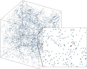
We first consider a typical collision process between two particles with/without Coulomb repulsion. In two different cases, the particle pairs are released in the turbulence with the same initial conditions and different charge parameters ( ${\kappa _q} = 0$ and
  ${\kappa _q} = 1.13$). Then particle motions in both cases are evolved to show the influence of Coulomb repulsion. Figure 1(a) displays the trajectories of the neutral and charged particle pairs as blue and red lines. Figure 1(b,c) illustrates the corresponding temporal evolution of the radial relative velocity,
  ${v_{rel}}( = ({\boldsymbol{v}_i} - {\boldsymbol{v}_j})\boldsymbol{\cdot }({\boldsymbol{r}_i} - {\boldsymbol{r}_j})/|{\boldsymbol{r}_i} - {\boldsymbol{r}_j}|)$, and the interparticle distance,
  ${r_{rel}}( = |{\boldsymbol{r}_i} - {\boldsymbol{r}_j}|)$. After being released, two neutral particles have a relative inward velocity, so they start to approach each other and eventually collide (inset of figure 1a). In this case, due to the weak adhesive force, the colliding particles will rebound, which corresponds to the jump of the relative velocity
  ${v_{rel}}$ from a negative value (inward) to a positive one (outward). As mentioned in § 2.3, the collision process is fully resolved on an ultra-fine collision time step
  $d{t_C}$ and presented in figure 1(d,e). Because the fluid time step
  $d{t_F}$ is much larger than
  $d{t_C}$, the rapid change of
  ${v_{rel}}$ looks like a discontinuous jump in figure 1(b). For the charged particles, the trajectories coincide with the neutral ones at the beginning, but the relative velocity decreases more rapidly when particles are getting closer. Since the initial inward velocity is not large enough to overcome the Coulomb repulsion,
  ${v_{rel}}$ reduces to zero before the particles can contact. Then
  ${v_{rel}}$ becomes positive, and the interparticle distance starts to rise. Consequently, the collision is suppressed.

Figure 1. (a) Centroid trajectories of two particles in both the neutral (blue,  $St\; = \; 1,\; {\kappa _q} = 0$) and the charged case (red,
  $St\; = \; 1,{\kappa _q} = 1.13$). In the inset, two colliding particles in the neutral case are displayed as grey spheres with their centroids enlarged. Temporal evolution of (b) the radial relative velocity
  ${v_{rel}}$ and (c) the relative distance
  ${r_{rel}}$ between two particles on the fluid time step
  $d{t_F}$. The collision moment in the neutral case is shown as the vertical green dash line, and the horizontal black dash line denotes
  ${v_{rel}} = 0$. Temporal evolution of (d) the radial relative velocity
  ${v_{rel}}$ and (e) the normalized relative distance
  ${r_{rel}}/{d_p}$ between two colliding particles on the ultra-fine collision time step
  $d{t_C}$. The adhesion parameter
  $Ad$ equals 0.14 for both cases.
The results indicate that two competing factors determine whether a collision event will happen, i.e. the incident kinetic energy and the Coulomb repulsion. If the incident kinetic energy is large enough to overcome the Coulomb repulsion, the approaching particles will collide. Otherwise, the collision will be prevented. Besides, our previous results have shown that the contact forces and torques will determine the sticking/rebound behaviours once particles are in contact (Chen, Li & Yang Reference Chen, Li and Yang2015). Therefore, in the following sections, both the collision frequency and the sticking probability of charged particles will be discussed to show the impact on particle agglomeration.
3.2. Effect of Coulomb repulsion on collision frequency
We start with the effect of Coulomb repulsion on the collision frequency. In this section, 10 000 particles are first randomly distributed in the flow field with no overlap. The initial velocity of each particle is set equal to the local fluid velocity. Then particles start to transport in the turbulence and collide with each other. Since the adhesion force is intentionally set to be weak  $(Ad= 0.14)$, almost all the collisions will result in a rebound. Eventually, an equilibrium state is reached, where both the spatial distribution and the collision frequency remain steady. By varying
  ${\kappa _q}$ and
  $St$, the impact of the long-range Coulomb repulsion and particle inertia on the collision frequency is investigated.
The collision kernel,  $\varGamma$, is employed to measure the collision frequency (Smoluchowski Reference Smoluchowski1916), which is defined as
 \begin{equation}\varGamma = \frac{{2{{\dot{N}}_c}}}{{n_0^2}}.\end{equation}
Here,  ${\dot{N}_c}$ is the collision rate per unit volume,
  ${n_0} = {N_p}/{L^3}$ is the average particle number concentration. For non-inertial particles, the interparticle collision is caused by the local fluid shear rate (Saffman & Turner Reference Saffman and Turner1956). The corresponding collision kernel,
  ${\varGamma _0}$, equals
 \begin{equation}{\varGamma _0} = {(8{\rm \pi}\epsilon /15\nu )^{1/2}}{(2{r_p})^3}.\end{equation}
The value of  ${\varGamma _0}$ is adopted as a baseline for normalization hereafter.
The temporal evolution of the normalized collision kernel  $\varGamma /{\varGamma _0}$ for different charge parameters
  ${\kappa _q}$ and
  $St = 1$ is plotted in figure 2(a). In each run,
  $\varGamma /{\varGamma _0}$ rises in the initial stage and then fluctuates around the equilibrium value. The equilibrium value,
  ${\varGamma _{eq}}/{\varGamma _0}$, is then obtained by averaging over 12 large-eddy turnover times. Figure 2(b) plots the normalized equilibrium collision kernel
  ${\varGamma _{eq}}/{\varGamma _0}$ as a function of
  $St$ for different
  ${\kappa _q}$. The value of
  ${\varGamma _{eq}}/{\varGamma _0}$ decreases continuously with the increase of
  ${\kappa _q}$, which results from the fact that the Coulomb force always repels approaching particles. Moreover, for neutral particles,
  ${\varGamma _{eq}}/{\varGamma _0}$ decreases monotonically as
  $St$ increase, whereas for strongly charged particles,
  ${\varGamma _{eq}}/{\varGamma _0}$ rises as
  $St$ increases
  $({\kappa _q} = 0.635\;\textrm{and}\;1.13)$. The reverted monotonicity suggests that the dominant collision mechanism has changed.

Figure 2. (a) Temporal evolution of the normalized collision kernel  $\varGamma /{\varGamma _0}$ for different charge parameters
  ${\kappa _q}$ with
  $St\; = \; 1$. The equilibrium values are displayed as horizontal black dash lines. (b) The equilibrium collision kernel as a function of Stokes number
  $St$ for different charge parameter
  ${\kappa _q}$. The adhesion parameter
  $Ad$ equals 0.14 for all cases. The legend in (a) also applies to (b).
To further reveal the transition of the monotonicity, we adopt the decomposition analysis proposed by Voßkuhle et al. (Reference Voßkuhle, Pumir, Lévêque and Wilkinson2014) and Pumir & Wilkinson (Reference Pumir and Wilkinson2016), in which the collision enhancement is attributed to two effects: preferential concentration and the sling effect. The collision kernel is decomposed as
 \begin{equation}{\varGamma _{eq}} = {\varGamma _{pref}} + {\varGamma _{sling}}.\end{equation}
Here,  ${\varGamma _{pref}}$ and
  ${\varGamma _{sling}}$ are the contributions from preferential concentration and the sling effect, respectively.
Due to preferential concentration, particles tend to cluster in the straining regions outside the vortical structures. Without the sling effect, the particle velocity field is single valued, so the trajectories of nearby particles are approximately parallel (Bewley et al. Reference Bewley, Saw and Bodenschartz2013). In this case, collisions happen when adjacent particles are moving along their trajectories and collide with each other due to the local fluid shear rate (figure 3a). According to Voßkuhle et al. (Reference Voßkuhle, Pumir, Lévêque and Wilkinson2014), the clustering of particles in straining zones only has minor impacts on their relative velocity, so the collision kernel between clustering particles can still be given by  ${\varGamma _0}$. As a result,
  ${\varGamma _{pref}}$ can be computed by
 \begin{equation}{\varGamma _{pref}} = {\varGamma _0} \cdot g({d_p}),\end{equation}
where  $g({d_p})$ is the RDF at contact.

Figure 3. Schematics of (a) preferential concentration and (b) the sling effect.
When encountering intermittent fluctuations, particle clouds from different regions could quickly interpenetrate each other, resulting in the crossing of particle trajectories (figure 3b). The formation of such singularities in the particle velocity field (or the caustics) is related to large relative velocity and further enhances interparticle collisions. The contribution of the sling effect,  ${\varGamma _{sling}}$, is then computed by subtracting
  ${\varGamma _{pref}}$ from
  ${\varGamma _{eq}}$.
To measure  ${\varGamma _{pref}}/{\varGamma _0}$, we calculate the RDF at contact
  $g({d_p})$ for each case. Figure 4(a) displays
  ${\varGamma _{pref}}/{\varGamma _0}( = g({d_p}))$ as a function of St for different charge parameter
  ${\kappa _q}$. For the neutral case,
  ${\varGamma _{pref}}/{\varGamma _0}$ shows a monotonically decreasing trend on St and experiences its peak when St is around unity, which is consistent with previous DNS results (Wang et al. Reference Wang, Wexler and Zhou2000). For charged particles, the presence of the repulsive Coulomb force is found to reduce
  ${\varGamma _{pref}}/{\varGamma _0}$ and mitigates the preferential concentration. Specifically, for the strongest charge case
  $({\kappa _q} = 1.13)$, the
  ${\varGamma _{pref}}/{\varGamma _0}$ curve almost collapses to a straight line for
  ${\varGamma _{pref}}/{\varGamma _0} = 1$. This implies that the local particle concentration at contact is close to the average concentration
  ${n_0}$ and only has a limited effect on collision enhancement. Besides,
  ${\varGamma _{pref}}/{\varGamma _0}$ for larger St decreases slower as
  ${\kappa _q}$ increase, because particles with a larger St have a weaker tendency of accumulation and
  ${\varGamma _{pref}}/{\varGamma _0}$ is quite small even for neutral particles.

Figure 4. Normalized collision kernel caused by (a) preferential concentration  ${\varGamma _{pref}}/{\varGamma _0}$ and (b) the sling effect
  ${\varGamma _{sling}}/{\varGamma _0}$. (c) Ratio of the collision contribution by preferential concentration. The horizontal green dash line represents
  ${\varGamma _{pref}}/{\varGamma _0} = 0.5$. The adhesion parameter
  $Ad$ equals 0.14 for all cases. The legend in (a) also applies to (b,c).
Figure 4(b) illustrates  ${\varGamma _{sling}}/{\varGamma _0}$ as a function of St for different
  ${\kappa _q}$. For a fixed
  ${\kappa _q}$, since the sling becomes more likely to happen for larger particle inertia,
  ${\varGamma _{sling}}/{\varGamma _0}$ shows an increasing dependence on Stokes number. However,
  ${\varGamma _{sling}}$ saturates as St further increases, which could be attributed to the influence of the limited Reynolds number
  $(R{e_\lambda } = 74.8)$ in this study. As a result, there are no larger-scale motions to further actuate denser particles. For a fixed St,
  ${\varGamma _{sling}}/{\varGamma _0}$ is observed to also drop as
  ${\kappa _q}$ increases, but
  ${\varGamma _{sling}}/{\varGamma _0}$ drops much slower compared to
  ${\varGamma _{pref}}/{\varGamma _0}$, which might be attributed to the large relative velocity between slinging particles. Since the sling effect brings particles together from different regions, the corresponding collisions are more energetic and thus less influenced by the Coulomb repulsion.
We then plot the fraction of the collision contribution due to  ${\varGamma _{pref}}$ in figure 4(c). As can be seen, when St and
  ${\kappa _q}$ are small, the preferential concentration is the dominant mechanism that causes interparticle collisions, whereas the sling effect prevails when St or
  ${\kappa _q}$ increases. Consequently, as
  ${\kappa _q}$ increases, the major contributor of
  ${\varGamma _{eq}}$ changes from
  ${\varGamma _{pref}}$ to
  ${\varGamma _{sling}}$, which explains the monotonicity inversion of the dependence on St in figure 2(b).
3.3. Effect of Coulomb repulsion on collision velocity
Apart from the collision frequency, another key issue in particle agglomeration is the collision velocity, which is of importance in determining the agglomerate formation (Chen et al. Reference Chen, Li and Marshall2019a) and the collision-induced breakage (Liu & Hrenya Reference Liu and Hrenya2018; Chen & Li Reference Chen and Li2020).
We record the normal collision velocity  ${v_c}$ of each collision event to obtain statistics. Since
  ${v_c}$ differs by more than two orders of magnitude, we divide the collision velocity space into ten sub-intervals on a log scale, with
  ${v_{c,i}}$ being the median collision velocity of the ith sub-interval. Then, all the collision events are classified into the sub-intervals by their colliding velocity. The value of
  ${N_{c,i}}({v_{c,i}})$ is the number of collision events in the ith sub-interval, which is called the grouped collision events number hereafter. From (3.1), the relationship between the collision kernel
  ${\varGamma _{eq}}$ and the grouped collision events number
  ${N_{c,i}}({v_{c,i}})$ can be written as
 \begin{equation}{\varGamma _{eq}} = \frac{2}{{n_0^2 \cdot \Delta T}}\mathop \sum \limits_i {N_{c,i}}({v_{c,i}}).\end{equation}
Figure 5 illustrates the distribution of grouped collision events number  ${N_{c,i}}({v_{c,i}})$ of different charge parameter
  ${\kappa _q}$ and St. As shown in figure 5(a), when particle charge increases,
  ${N_{c,i}}({v_{c,i}})$ reduces for all
  ${v_{c,i}}$. For collisions with small
  ${v_{c,i}}$, since the collision kinetic energy is not large enough to overcome the Coulomb repulsion,
  ${N_{c,i}}({v_{c,i}})$ decreases drastically, while
  ${N_{c,i}}({v_{c,i}})$ for large
  ${v_{c,i}}$ is less affected.

Figure 5. Number of grouped collision events  ${N_{c,i}}$ as a function of collision velocity
  ${v_{c,i}}$ for different charge parameters
  ${\kappa _q}$ for (a) St = 1, (b) St = 2, (c) St = 4 and (d) St = 6. The adhesion parameter
  $Ad$ equals 0.14. Results are taken over
  $\Delta T = 12{T_e}$. The legend in (a) applies to all panels.
As St increases, due to the transition of the dominant mechanism from preferential concentration to the sling effect, the distribution shifts towards the direction of larger  ${v_{c,i}}$ (figure 5b,c). The collisions of particles with a larger
  $St$ are thus less sensitive to the increases of
  ${\kappa _q}$.
3.4. Sticking probability for charged particles
Once particles collide with each other, it is of great concern to predict whether particles will stick or rebound. For microparticles, the adhesion due to van der Waals force dominates and leads to agglomerate formation (Chen et al. Reference Chen, Li and Yang2015; Fang et al. Reference Fang, Wang, Zhang, Wei, Wu and Sun2019). In the previous study of Chen et al. (Reference Chen, Li and Marshall2019a), the mean sticking probability  $\theta $ has been successfully modelled for neutral particles, and the modified adhesion parameter,
  $A{d_n}$, is proposed to describe the competition between van der Waals adhesion and particle inertia.
Although both translational and rotational motions are considered in the present study, it is the normal contact force that plays a major role in determining the sticking and detachment behaviour. Thus, in this section, the sticking probability is modelled by analysing the momentum equation of particles. We first estimate the relative importance of three forces in a collision process, i.e. the fluid drag force  ${F^{drag}}$, the normal elastic force
  ${F^{ne}}$ and Coulomb force
  ${F^E}$. From (2.20), the ratios between different forces scale as
 \begin{equation}\frac{{{F^{drag}}}}{{{F^{ne}}}}\sim \frac{1}{{Ad \cdot St}},\quad \frac{{{F^E}}}{{{F^{ne}}}}\sim \frac{{{\kappa _q}}}{{Ad}}.\end{equation}
By using parameters of typical solid microparticles (table 2), these ratios are much smaller than unity, indicating that the contact force prevails once particles contact each other. The effects of the drag force and Coulomb force is thus negligible in collision analysis. The modified adhesion parameter,  $A{d_n}$, which is derived from the governing equation for head-on collisions (Chen et al. Reference Chen, Li and Marshall2019a; Chen, Liu & Li Reference Chen, Liu and Li2019b), is employed to model the sticking probability
 \begin{equation}A{d_n} = \frac{\nu }{{{\rho _p}v_c^2{r_p}}}.\end{equation}
 In order to find the relation between  $\theta $ and
  $A{d_n}$, simulations with different
  $St( = 1,2,4,6)$ and
  $Ad( = 11.1,,22.2)$ for both neutral
  $({\kappa _q} = 0)$ and charged particles
  $({\kappa _q} = 1.13)$ are run. Again, the collision events in each case are classified into different groups (sub-intervals) by the collision velocity
  ${v_{c,i}}$. For each group of collision events, the grouped sticking probability
  $\theta ({v_{c,i}})$ is computed by
 \begin{equation}\theta ({v_{c,i}}) = {N_{s,i}}({v_{c,i}})/{N_{c,i}}({v_{c,i}}).\end{equation}
Here,  ${N_{s,i}}({v_{c,i}})$ is the grouped sticking events number, and
  ${N_{c,i}}({v_{c,i}})$ is the grouped collision event number. The modified adhesion parameter for each group is then calculated by
  $A{d_n}({v_{c,i}}) = \nu /({\rho _p}v_{c,i}^2{r_p})$. In the previous study by Chen et al. (Reference Chen, Li and Marshall2019a), the mean collision velocity
  ${v_{cn}}$ of all the collisions is adopted to define the mean adhesion number, which is later used to model the mean sticking probability. In the present study, by using the median collision velocity
  ${v_{c,i}}$ of the ith velocity sub-interval, the modified adhesion parameter
  $A{d_n}({v_{c,i}})$ can be used for a more precise prediction of the grouped sticking probability
  $\theta ({v_{c,i}})$.
To ensure reliable statistics, only the data points  $(\theta ({v_{c,i}}),A{d_n}({v_{c,i}}))$ with enough collision events
  $({N_{c,i}}({v_{c,i}}) \ge 150)$ are shown in figure 6. Despite different
  $St$ and
  ${\kappa _q}$, the data collapse on the same curve, which validates our assumption that only
  $A{d_n}({v_{c,i}})$ controls this process. When
  $A{d_n}$ is small, the interparticle adhesion is weak. Particles will always rebound after each collision, so the sticking probability
  $\theta ({v_{c,i}})$ is zero. As
  $A{d_n}({v_{c,i}})$ further increases and exceeds a critical value
  $A{d_C}$,
  $\theta $ quickly steps up and approaches unity, indicating an adhesion-dominated regime where particles will simply hit and stick. To capture this step-up behaviour, we employ the logistic function for a smooth approximation
 \begin{equation}\theta (A{d_n}) = \frac{1}{{1 + exp [ - {a_\theta }(\log A{d_n} - \log A{d_C})]}}.\end{equation}
Here,  $A{d_C}$ is the critical value of
  $A{d_n}({v_{c,i}})$ that describes where
  $\theta ({v_{c,i}})$ steps up, and
  ${a_\theta }$ characterizes the steepness of this transition. The fitting result is displayed as the blue curve in figure 6, with
  ${a_\theta } = 18.71$ and
  $A{d_C} = 58.7$. Equation (3.9) is determined by the collision equation and is independent of the flow conditions. Once we obtain the relative velocity at contact from ghost particle simulation or theoretical derivation, the fitted results can be used empirically to predict the sticking probability.

Figure 6. Dependence of the grouped sticking probability  $\theta ({v_{c,i}})$ on the modified adhesion parameter
  $A{d_n}({v_{c,i}})$.
3.5. Combined effect of Coulomb repulsion and interparticle adhesion
In this section, we consider the combined effect of Coulomb repulsion and interparticle adhesion on particle agglomeration. Simulations are run with fixed  $Ad = 22.2$ and different St and
  ${\kappa _q}$. The interparticle adhesion here is strong enough to enable agglomerate formation. In each case, particles will undergo frequent collisions to form non-spherical agglomerates. A snapshot of typical agglomerate structures is given in figure 7(a). As time increases, more particles will exist in the form of agglomerates (figure 7b), which reduces the particle concentration. As a result, for adhesive particles, the collision kernel calculated by (3.1) will gradually decrease and deviate from the equilibrium collision kernel
  ${\varGamma _{eq}}$ (figure 7c).

Figure 7. (a) Snapshot of typical agglomerate structures. The colour bar represents the number of primary particles in each agglomerate. (b) Temporal evolution of the fraction of particles,  $P(A)$, existing in the form of agglomerates containing A primary particles for
  $St = 1$,
  ${\kappa _q} = 0.071$ and
  $Ad = 22.2$. (c) Comparison of the temporal evolution of the normalized collision kernel
  $\varGamma /{\varGamma _0}$ between
  $Ad = 0.14/22.2$ for
  $St = 1$ and
  ${\kappa _q} = 0.071$.
We use the number of sticking events instead of the collision kernel to quantify the agglomeration process. The total number of sticking events,  ${N_s}$, is given by
 \begin{equation}{N_s} = \sum\limits_i {{N_{s,i}}({v_{c,i}})} = \sum\limits_i {{N_{c,i}}({v_{c,i}}) \cdot \theta ({v_{c,i}})} .\end{equation}
Here,  ${N_{s,i}}({v_{c,i}})$ is the number of the grouped sticking events with a median collision velocity
  ${v_{c,i}}$, which could be further estimated by
  ${N_{s,i}}({v_{c,i}}) = {N_{c,i}}({v_{c,i}}) \cdot \theta ({v_{c,i}})$ from (3.8). Figure 8(a) illustrates the number of grouped collision events
  ${N_{c,i}}({v_{c,i}})$ for different
  ${\kappa _q}$ with the fixed
  $St = 1$. The grouped sticking probability
  $\theta ({v_{c,i}})$ calculated by (3.9) is also shown as the blue curve (right y-axis). We then estimate the sticking event number
  $N_{s,i}^{est}({v_{c,i}})$ from (3.10) and plot the results as open symbols in figure 8(b). In comparison, the number of grouped sticking events
  ${N_{s,i}}({v_{c,i}})$ directly taken from the simulations is also plotted as closed symbols. The reasonable agreement between
  $N_{s,i}^{est}({v_{c,i}})$ and
  ${N_{s,i}}({v_{c,i}})$ validates the applicability of (3.9) in charged particle agglomeration. If the physical properties of the particle (e.g. surface energy density, density, radius, etc.) are known a priori, one can predict the sticking events number
  ${N_s}$ from (3.10) by only conducting simulations for non-adhesive charged particles and then calculating the sticking probability, which will avoid expensive computations resolving interparticle collisions at an ultra-fine collision time step.

Figure 8. (a) Number of grouped collision events  ${N_{c,i}}({v_{c,i}})$ for different charge parameters
  ${\kappa _q}$ and
  $St = 1$. The
  $\theta ({v_{c,i}}) - {v_{c,i}}$ curve is calculated from (3.9). (b) Comparison of the grouped sticking events number
  ${N_{s,i}}({v_{c,i}})$ from simulation and the estimated value
  $N_{s,i}^{est}({v_{c,i}})$ by (3.10) for different charge parameters
  ${\kappa _q}$ and
  $St = 1$.
To show the combined effect of Coulomb repulsion and interparticle adhesion, figure 9(a) plots  ${N_{c,i}}$ and
  ${N_{s,i}}$ directly taken for
  $St = 1$ as open and closed symbols, respectively. For a fixed
  ${\kappa _q}$, when the collision velocity
  ${v_{c,i}}$ is small,
  ${N_{s,i}}$ coincides with
  ${N_{c,i}}$, indicating that all collision events lead to sticking events. As
  ${v_{c,i}}$ further increases and exceeds a critical velocity
  ${v_{crit}}$, the corresponding sticking probability
  $\theta $ decreases to zero. In this case, even though the collision events number
  ${N_{c,i}}$ is still large, the number of sticking events
  ${N_{s,i}}$ goes down quickly. Therefore, the sticking probability
  $\theta $ acts like a low-pass filter, which only allows particles with a low collision velocity
  ${v_c}$ to stick together. For the case shown in figure 9(a), taking the critical adhesion parameter
  $A{d_C} = 58.7$ into (3.7) thus yields the critical velocity
  ${v_{crit}}/u^{\prime} = 0.14$. If the interparticle adhesion becomes stronger,
  ${v_{crit}}$ will also increase, resulting in the occurrence of more sticking events. Moreover, when
  ${\kappa _q}$ increases,
  ${N_{c,i}}$ decreases significantly for small
  ${v_{c,i}}$, which is consistent with the results in figure 5. Since particles with large
  ${v_c}$ are more likely to overcome the energy barrier and collide, the effect of Coulomb repulsion is similar to a high-pass filter.

Figure 9. Number of collision events  ${N_{c,i}}$ and sticking events
  ${N_{s,i}}$ for different charge parameters
  ${\kappa _q}$ and (a) St = 1, (b) St = 2, (c) St = 4 and (d) St = 6. Results are taken in a period of time
  $\Delta T = 100$.
  $Ad = 22.2$ is fixed for all cases. The legend in (a) applies to all panels.
To summarize, when the effects of Coulomb repulsion and interparticle adhesion both exist, collisions with low  ${v_c}$ are suppressed by the Coulomb repulsion, while particles with high
  ${v_c}$ will rebound after collisions. Eventually, if one collision leads to sticking, the collision velocity
  ${v_c}$ is more likely to lie within a moderate range, which corresponds to the peaks of
  ${N_{s,i}}$ curves in figure 9(a). This conclusion also applies to different Stokes numbers in figure 9(b,d). It should be noted that, as
  $St$ further increases, the collisions become so energetic that most particles will rebound after collisions. As a result, although the number of collision events
  ${N_{c,i}}$ for large
  $St$ are less influenced by Coulomb repulsion, there are still few sticking events that actually contribute to agglomerate formation (figure 9c,d). Specifically, for different cases with
  $St = 6$, due to the low sticking probability, almost all the particles
  $\mathrm{(\ \gt }99\,\%)$ still exist in the form of singlets, doublets and triplets at the end of the simulations
  $(t = 100)$.
Finally, it is of importance to consider the agglomerate structure in our simulation (figure 7a), which is closely related to agglomerate migration (Sorensen Reference Sorensen2010) and collision dynamics (Chen et al. Reference Chen, Li and Marshall2019a). The gyration radius,  ${R_g}$, and the fractal dimension,
  ${D_f}$, are often employed to describe the size and compactness of a non-spherical agglomerate. Their definitions are given by
 \begin{equation}{R_g} = {\left( {\sum\limits_{i = 1}^A {({\boldsymbol{r}_i} - {\boldsymbol{r}_C})/A} } \right)^{1/2}},\end{equation}
 \begin{equation}A = {k_f}{({R_g}/{r_p})^{{D_f}}}.\end{equation}
Here, A is the number of primary particles contained in one agglomerate,  ${\boldsymbol{r}_C} = \sum\nolimits_{i = 1}^A {{\boldsymbol{r}_i}/A} $ is the mass centre of the agglomerate and
  ${k_f}$ is the fractal pre-factor. Figure 10 plots the dimensionless gyration radius
  ${R_g}/{r_p}$ as a function of A for different cases. It can be found that, for a fixed Stokes number, the results for different
  ${\kappa _q}$ collapse on to the same line. This implies that the Coulomb force does not modify the agglomerate structures. This could be attributed to the point-charge model in the present study. Since the charge is assumed to be located at the centroid of particles, the effect of Coulomb force will always be isotropic and repulsive, which does not significantly adjust collision angle or contact point. As a result, the Coulomb force only reduces the agglomeration rate but has no obvious influence on the formed structures. It is worth noting that, when considering the influence of particle polarization, this process could be very different. As two polarized particles approach each other, the dipole force could be attractive in some directions but repulsive in other directions. Consequently, polarized particles tend to stick at certain positions and change the agglomerate structure. This phenomenon is beyond the scope of the present study and left for future investigations.

Figure 10. Dimensionless gyration radius  ${R_g}/{r_p}$ as a function of the number of primary particles A contained in each agglomerate for (a)
  $\; St = 1$, (b)
  $\; St = 2$, (c)
  $\; St = 4$ and (d)
  $\; St = 6$. Only data points with enough samples are plotted
  $(n(A) \ge 5)$. The legend in (a) applies to all panels.
The fractal dimension  ${D_f}$ and the pre-factor
  ${k_f}$ for different
  $St$ are obtained by fitting (3.12). The fitting parameters are listed in table 3. The fitted fractal dimension
  ${D_f}$ is within the range of
  $1.25- 1.41$. In turbulent agglomeration, small loose agglomerates are generally formed after initial particle–particle collisions. When these loose agglomerates grow larger, the structures will densify as a result of frequent collisions and restructuring (Selomulya et al. Reference Selomulya, Amal, Bushell and Waite2001; Waldner et al. Reference Waldner, Sefcik, Soos and Morbidelli2005; Ruan, Chen & Li Reference Ruan, Chen and Li2020) and the fractal dimension will be around 1.7 to 2. In our simulation, however,
  ${D_f}$ is quite small, which means the agglomeration is still in the very early stage.
Table 3. Fitting parameters for agglomerate structure.

4. Conclusions
By conducting DNS–DEM simulations, the dynamic process of charged particle transport and agglomerate formation is studied in homogeneous isotropic turbulence. The effect of Coulomb repulsion on collision frequency is quantified by calculating the normalized equilibrium collision kernel  ${\varGamma _{eq}}/{\varGamma _0}$. By decomposing
  ${\varGamma _{eq}}/{\varGamma _0}$, the dominant collision mechanism is found to change from preferential concentration to the sling effect as
  $St$ and
  ${\kappa _q}$ increase. When particles are at contact, the contact force plays a dominant role, and the modified adhesion parameter
  $A{d_n}$ can successfully predict the sticking probability
  $\theta $. Besides, due to the combined effect of Coulomb repulsion and interparticle adhesion, particles with a moderate collision velocity are more likely to collide and stick, which largely contributes to particle agglomeration. Furthermore, in our study where the Coulomb force is considered but the effect of higher-order multipoles is omitted, the agglomerate structures formed by charged and neutral particles show no obvious differences.
To understand the impact of Coulomb force from a broader physical picture, it would be beneficial to discuss the relative importance of Coulomb repulsion compared to other interactions in the process of particle agglomeration. Here, we follow Di Renzo & Urzay (Reference Di Renzo and Urzay2018) and compare the magnitudes of different velocities caused by turbulence and the Coulomb force. Assuming the characteristic separation distance  ${r_{sep}}$ between like-charged particles varies in the range
  $(1\sim 100)\eta $, the electrical migration velocity induced by local particle clusters can be given by
 \begin{equation}{u_{el}}\sim \frac{{{n_0}r_{sep}^3{q^2}/(4{\rm \pi}{\varepsilon _0}r_{sep}^2)}}{{3{\rm \pi}\mu {d_p}}}.\end{equation}
 Taking the parameters from table 2 yields  ${u_{el}}/{u_\eta }\mathrm{\ \mathbin{\lower.3ex\hbox{$\buildrel\lt \over {\smash{\scriptstyle\sim}\vphantom{_x}}$}}\ }{10^{ - 1}}$, which means the present study lies within the weak electrical interaction regime. In this case, Coulomb repulsion does not alter the particle–turbulence interaction on a large scale, but only modifies particle behaviour at a short separation distance (figure 1a). The disordered particle distribution can thus be considered amorphous, which is physically relevant for charged solid particles suspended in gaseous turbulence (Lu et al. Reference Lu, Nordsiek, Saw and Shaw2010; Di Renzo & Urzay Reference Di Renzo and Urzay2018). In comparison, in colloidal systems, the repulsive force could become dominant and repel all the approaching particles. The system thus transits to the crystal state (or the glass state), where the particles assemble in an organized way (Chu & Lin Reference Chu and Lin1994; Fortov et al. Reference Fortov2003; Klix, Royall & Tanaka Reference Klix, Royall and Tanaka2010; Gupta et al. Reference Gupta, Chaudhuri, Bec and Ray2018). As a result, the system is stabilized by the strong repulsion, and the interparticle collision is entirely suppressed.
Another common interaction is the short-range hydrodynamic interaction, or the lubrication force, which is omitted in the present study. The lubrication force is
 \begin{equation}{F_{lub}} = \frac{{3{\rm \pi}\mu r_p^2}}{{2h}}\left( { - \frac{{\textrm{d}h}}{{\textrm{d}t}}} \right).\end{equation}
Here,  $\mu $ is the dynamic viscosity of the fluid,
  ${r_p}$ is the particle radius and
  $h = |{\boldsymbol{x}_i} - {\boldsymbol{x}_j}|- 2{r_p}$ is the distance between the surfaces of two particles. The approaching velocity,
  $ - \textrm{d}h/\textrm{d}t$, can be estimated by the collision velocity
  ${v_c}$. Based on Marshall (Reference Marshall2011), the suggested initial distance and the minimum distance of
  ${F_{lub}}$ are given by
  ${h_{max}}\sim 0.01{r_p}$ and
  ${h_{min}}\sim {10^{ - 4}}{r_p}$. The energy barrier due to the lubrication force can be estimated by
 \begin{equation}\Delta {E_{lub}} = \int_{{h_{min}}}^{{h_{max}}} {{F_{lub}}\,\textrm{d}h} \approx \frac{{3{\rm \pi}\mu r_p^2{v_c}}}{2}\textrm{ln(}{h_{max}}/{h_{min}}\textrm{)}.\end{equation}
In comparison, the energy barrier caused by the Coulomb force is
 \begin{equation}\Delta {E_{Coul}} = \frac{{{q^2}}}{{4{\rm \pi}{\varepsilon _0}{d_p}}}.\end{equation}
In our simulation,  $\mu = {10^{ - 5}}\;\textrm{Pa} \cdot \textrm{s}$,
  ${r_p} = 10\;\mathrm{\mu }\textrm{m}$,
  ${v_c}\sim ({10^{ - 2}} - 1)\;\textrm{m}\;{\textrm{s}^{ - 1}}$. If a particle's charging density is of the order of
  $10\;\mathrm{\mu }\textrm{C}\;{\textrm{m}^{ - 2}}$ (or
  $q\sim {10^{ - 14}}\;\textrm{C}$), the energy barriers can be estimated as
  $\Delta {E_{lub}}\sim ({10^{ - 16}} - {10^{ - 14}})J$ and
  $\Delta {E_{Coul}}\sim ({10^{ - 14}} - {10^{ - 13}})J$. Thus, compared to Coulomb interaction, the short-range hydrodynamic interaction has a weaker impact. But under certain conditions of weak particle charge and large collision velocity, the short-range hydrodynamic interaction could become more important. In the present study, we focus on the impact of Coulomb repulsion, so the effect of the short-range hydrodynamic interaction is intentionally neglected.
In addition, as discussed in § 3.4, the contact force is found to play an essential role when particles contact each other. Here, we adopt the normal contact force as a typical measure of the contact interactions, which equals  ${F_{ne}} = 4{F_C}[{(a/{a_0})^3} - {(a/{a_0})^{3/2}}]$ (§ 2.2.4). The Coulomb force between two contacting particles is
  ${F_{Coul}} = {q^2}/(4{\rm \pi}{\varepsilon _0}|{\boldsymbol{x}_1} - {\boldsymbol{x}_2}{|^2})$ under the point-charge assumption. For physical relevant parameters given in table 2, the ratio
  ${F_{ne}}/{F_{Coul}}\sim O(10)$. Thus, the normal contact force prevails once interparticle collision happens.
Based on our results, there are several interesting directions for future investigations. First, in this study, we focus on the early-stage agglomeration process. In this stage, most particles exist in the form of singlets or small agglomerates. Particle behaviour still resembles that of single particles. If the agglomeration goes on, agglomerates will continue to grow larger. How these large agglomerates react to the turbulence is still unclear and remains to be resolved. Second, the present study adopts the point-charge model to include electrostatic interactions, and some important electrical effects are neglected. First of all, the charge transfer during frequent collisions (McCarty & Whitesides Reference McCarty and Whitesides2008; Jin & Marshall Reference Jin and Marshall2017; Kolehmainen et al. Reference Kolehmainen, Ozel, Boyce and Sundaresan2017) and the electrical breakdown (Matsuyama & Yamamoto Reference Matsuyama and Yamamoto1995; Soh et al. Reference Soh, Kwok, Liu and Whitesides2012) will significantly change the particle charge distribution and further affect the Coulomb force. In addition to the point-charge assumption, when particles are close to each other, the induced higher-order multipoles could have a significant impact on the particle behaviour. Consequently, particles could form chain-like structures, experience stronger clustering and probably encounter runaway growth (Ivelev et al. Reference Ivelev, Morfill and Konopka2002; Liu et al. Reference Liu, Marshall, Li and Yao2010; Lee et al. Reference Lee, Waitukaitis, Miskin and Jaeger2015; Kolehmainen et al. Reference Kolehmainen, Ozzel, Gu, Shinbrot and Sundaresan2018).
Moreover, the present study is limited to the same Reynolds number  $(R{e_\lambda } = 74.8)$. For neutral particles, the increase of
  $R{e_\lambda }$ has been reported to significantly affect both the spatial clustering and the relative velocity, and therefore enhances interparticle collisions (Wang et al. Reference Wang, Wexler and Zhou2000; Ireland et al. Reference Ireland, Bragg and Collins2016a,Reference Ireland, Bragg and Collinsb; Dou et al. Reference Dou, Bragg, Hammond, Liang, Collins and Meng2018). Hence, how charged particle dynamics could be modified in a broader range of
  $R{e_\lambda }$ may be worth pursuing in future studies.
Acknowledgements
We are grateful to Professor C. Sun at Tsinghua University, Professor R. Ni at Johns Hopkins University and Professor Y. Jin at Institute of Theoretical Physics, Chinese Academy of Sciences for fruitful discussions.
Funding
S.Q.L. acknowledges support from the National Natural Science Foundation of China (No. 51725601) and the NSFC-DFG Joint Program, China (No. 51761135126).
Declaration of interests
The authors report no conflict of interest.


