2.1 Governing equations

The governing equations for all simulations in this work are the dimensionless compressible Navier–Stokes equations for a Newtonian fluid. Applying conservation of mass, momentum and energy in three spatial directions $x_{i}$ ($i=1,2,3$) results in a system of five partial differential equations given by

(2.1)$$\begin{eqnarray}\displaystyle & \displaystyle \frac{\unicode[STIX]{x2202}\unicode[STIX]{x1D70C}}{\unicode[STIX]{x2202}t}+\frac{\unicode[STIX]{x2202}}{\unicode[STIX]{x2202}x_{k}}(\unicode[STIX]{x1D70C}u_{k})=0, & \displaystyle\end{eqnarray}$$

(2.2)$$\begin{eqnarray}\displaystyle & \displaystyle \frac{\unicode[STIX]{x2202}}{\unicode[STIX]{x2202}t}(\unicode[STIX]{x1D70C}u_{i})+\frac{\unicode[STIX]{x2202}}{\unicode[STIX]{x2202}x_{k}}(\unicode[STIX]{x1D70C}u_{i}u_{k}+p\unicode[STIX]{x1D6FF}_{ik}-\unicode[STIX]{x1D70F}_{ik})=0, & \displaystyle\end{eqnarray}$$

(2.3)$$\begin{eqnarray}\displaystyle & \displaystyle \frac{\unicode[STIX]{x2202}}{\unicode[STIX]{x2202}t}(\unicode[STIX]{x1D70C}E)+\frac{\unicode[STIX]{x2202}}{\unicode[STIX]{x2202}x_{k}}\left(\unicode[STIX]{x1D70C}u_{k}\left(E+\frac{p}{\unicode[STIX]{x1D70C}}\right)+q_{k}-u_{i}\unicode[STIX]{x1D70F}_{ik}\right)=0, & \displaystyle\end{eqnarray}$$

for total energy $E$, with Fourier’s heat flux $q_{k}$ and viscous stress tensor $\unicode[STIX]{x1D70F}_{ij}$ defined as

(2.4)$$\begin{eqnarray}\displaystyle & \displaystyle q_{k}=\frac{-\unicode[STIX]{x1D707}}{(\unicode[STIX]{x1D6FE}-1)M_{\infty }^{2}Pr\,Re}\frac{\unicode[STIX]{x2202}T}{\unicode[STIX]{x2202}x_{k}}, & \displaystyle\end{eqnarray}$$

(2.5)$$\begin{eqnarray}\displaystyle & \displaystyle \unicode[STIX]{x1D70F}_{ik}=\frac{\unicode[STIX]{x1D707}}{Re}\left(\frac{\unicode[STIX]{x2202}u_{i}}{\unicode[STIX]{x2202}x_{k}}+\frac{\unicode[STIX]{x2202}u_{k}}{\unicode[STIX]{x2202}x_{i}}-\frac{2}{3}\frac{\unicode[STIX]{x2202}u_{j}}{\unicode[STIX]{x2202}x_{j}}\unicode[STIX]{x1D6FF}_{ik}\right). & \displaystyle\end{eqnarray}$$

Throughout this work the coordinates $x_{i}$ ($i=1,2,3$) are referred to as $(x,y,z)$ for the streamwise, bottom wall-normal and spanwise directions, respectively, with corresponding velocity components $(u,v,w)$. The equations are non-dimensionalised by free-stream velocity, density and temperature $(U_{\infty }^{\ast },\unicode[STIX]{x1D70C}_{\infty }^{\ast },T_{\infty }^{\ast })$, with a characteristic length based on the displacement thickness $\unicode[STIX]{x1D6FF}^{\ast }$ of the boundary layer imposed at the inlet. Further details of the boundary-layer initialization are given in § 3.1. Free-stream Mach number, Prandtl number and ratio of specific heat capacity for air are taken to be $M_{\infty }=2$, $Pr=0.72$ and $\unicode[STIX]{x1D6FE}=1.4$, respectively. Reynolds number based on the inlet displacement thickness is set as $Re_{\unicode[STIX]{x1D6FF}^{\ast }}=750$ throughout. The dynamic viscosity $\unicode[STIX]{x1D707}(T)$ is computed by Sutherland’s law

(2.6)$$\begin{eqnarray}\unicode[STIX]{x1D707}(T)=T^{3/2}\left(\frac{1+{\displaystyle \frac{T_{s}}{T_{\infty }}}}{T+{\displaystyle \frac{T_{s}}{T_{\infty }}}}\right),\end{eqnarray}$$

with reference and Sutherland temperatures taken to be $T_{\infty }=288.0~\text{K}$ and $T_{s}=110.4~\text{K}$. For an ideal Newtonian fluid, pressure can be calculated through the equation of state such that

(2.7)$$\begin{eqnarray}P=(\unicode[STIX]{x1D6FE}-1)\left(\unicode[STIX]{x1D70C}E-\frac{1}{2}\unicode[STIX]{x1D70C}u_{i}u_{i}\right)=\frac{1}{\unicode[STIX]{x1D6FE}M_{\infty }^{2}}\unicode[STIX]{x1D70C}T.\end{eqnarray}$$

Throughout this work wall-normal skin friction $C_{f}$ is calculated as

(2.8)$$\begin{eqnarray}C_{f}=\frac{\unicode[STIX]{x1D70F}_{w}}{\frac{1}{2}\unicode[STIX]{x1D70C}_{\infty }U_{\infty }^{2}},\end{eqnarray}$$

for a wall shear stress

(2.9a,b)$$\begin{eqnarray}\unicode[STIX]{x1D70F}_{w}=\unicode[STIX]{x1D707}\left.\frac{\unicode[STIX]{x2202}u}{\unicode[STIX]{x2202}y}\right|_{y=0}\quad \text{or}\quad \unicode[STIX]{x1D70F}_{w}=\unicode[STIX]{x1D707}\left.\frac{\unicode[STIX]{x2202}u}{\unicode[STIX]{x2202}z}\right|_{z=0,L_{z}}\end{eqnarray}$$

depending on whether the quantity is being evaluated on the bottom wall $(\,y=0)$ or sidewalls $(z=0,L_{z})$ of the domain, for the width $L_{z}$ shown in figure 1.

2.2 Discretisation schemes

The high-order finite-difference code OpenSBLI (Jacobs, Jammy & Sandham Reference Jacobs, Jammy and Sandham2017; Lusher, Jammy & Sandham Reference Lusher, Jammy and Sandham2018) is used to perform the simulations, which uses the stencil-based Oxford parallel structured software (OPS) embedded domain-specific language (eDSL) (Reguly et al. Reference Reguly, Mudalige, Giles, Curran and McIntosh-Smith2014) for parallelisation. Validation of the OpenSBLI code for laminar shock-wave/boundary-layer interactions was shown in Lusher et al. (Reference Lusher, Jammy and Sandham2018) for a 2-D version of the present case. Spatial discretisation is performed by a 5th-order weighted essentially non-oscillatory (WENO) scheme, specifically the improved WENO-Z scheme introduced by Borges et al. (Reference Borges, Carmona, Costa and Don2008). WENO schemes are a robust and well-established method for numerical shock capturing, Gross & Fasel (Reference Gross and Fasel2016) is an example of a WENO scheme being applied to a wide range of laminar-transitional SBLI with comparison to experiments. The WENO reconstruction is performed in characteristic space to minimise oscillations and uses the local Lax–Friedrich flux-splitting method. Viscous, heat flux and metric terms are computed by standard 4th-order central differencing, replaced at domain boundaries by the 4th-order boundary scheme of Carpenter, Nordström & Gottlieb (Reference Carpenter, Nordström and Gottlieb1998). To minimise memory usage a low-storage explicit 3rd-order Runge–Kutta scheme is used for time advancement, in the form provided by Carpenter & Kennedy (Reference Carpenter and Kennedy1994).

3.1 Domain specification and physical parameters

For span-periodic simulations of SBLI, the standard method of generating an incident shock is to apply the inviscid Rankine–Hugoniot jump conditions on the upper or inlet boundary of the domain. For confined duct flows, this is not valid as it creates a non-physical interface between the sidewall boundary layers and the shock jump conditions on the upper surface. In this work, the oblique shock is generated by deflecting the flow with a no-slip ramp as shown in figure 1. Duct dimensions, aspect ratio and the length of the shock generating ramp are the primary considerations when selecting a computational domain. The domain must also be long enough in the streamwise direction to allow the central flow-reversal to fully develop. The baseline case is selected to have a one-to-one aspect ratio with non-dimensional dimensions of $(L_{x}\times L_{y}\times L_{z})=(550,175,175)$ as in table 1. As these are laminar simulations, a modest flow deflection of $\unicode[STIX]{x1D703}_{sg}=2.0^{\circ }$ is selected for all simulations to follow Katzer (Reference Katzer1989) unless otherwise stated. On the upper surface in figure 1, $L_{in}$, $L_{sg}$ and $L_{out}$ refer to the distance between the inlet and the shock generator, the length of the shock generator and the remaining distance to the outlet. For the baseline case, the shock generator starts at $x=45$, with $L_{sg}=300$ and $L_{out}=205$. For this $L_{sg}$, the trailing edge expansion fan generated at $x=345$ leaves through the outlet of the domain without impinging on the bottom wall. The effect of $L_{sg}$ on the central separation bubble is given in § 3.3. The other cases in table 1 correspond to the aspect ratio study in § 5.1 for aspect ratios between one-quarter and four.

Figure 1. Schematic of the computational domain. An oblique shock wave is generated by deflecting the oncoming flow with a ramp angled at $\unicode[STIX]{x1D703}_{sg}$ to the free stream. No-slip isothermal wall conditions are enforced on the bottom wall, both sidewalls and on the upper surface between $L_{sg}$ and $L_{out}$.

Table 1. Domain specification and grid distributions. Aspect ratio ($AR$) is defined as the ratio of duct width to height $(L_{z}/L_{y})$. A one-to-one aspect ratio is taken as the baseline configuration.

All of the simulations are performed at Mach 2, with a laminar boundary-layer profile imposed at the inlet of the domain. Imposing an inlet boundary-layer profile avoids a possible numerical singularity at the leading edge, and is more computationally efficient as the size of the domain is reduced. The profile is obtained via the similarity solution of the compressible boundary-layer equations (White Reference White2006). The Reynolds number based on the displacement thickness at the start of the computational domain is $Re_{\unicode[STIX]{x1D6FF}\ast }=750$. For the baseline configuration, a flow deflection of $\unicode[STIX]{x1D703}_{sg}=2^{\circ }$ is applied by the shock generator located at $x_{sg}=45$, giving an inviscid impingement point of $x=328$ for the incident shock. Reynolds number based on the distance from the leading edge of the plate to the impingement point is $Re_{x}=3\times 10^{5}$ as in one of the cases from Katzer (Reference Katzer1989). For the variation of incident shock strength in § 5.2, the location of the shock generator is shifted to maintain the same $Re_{x}$ at impingement. On the bottom and both sidewalls of the domain a no-slip isothermal condition is applied with a constant non-dimensional temperature of $T_{w}=1.676$ (4 s.f.), corresponding to the adiabatic wall temperature from the similarity solution. A zero-gradient condition is applied on the upper boundary over $L_{in}$ in figure 1 to maintain the free stream and sidewall boundary layers upstream of the shock generator. At $x_{sg}$ the upper surface becomes a no-slip wall with the same isothermal condition as on the bottom and sidewalls of the domain. The no-slip condition on the upper surface is maintained until the outlet. At the inlet and outlet, a pressure extrapolation and low-order extrapolation method are applied, respectively, to improve stability. No boundary layer is initialised on the shock generator; it is left to develop naturally during the initial stages of the simulation. An open condition upstream of the shock generator was selected to mimic experimental configurations where the free stream is incident on a shock generator plate.

In the corner regions, boundary-layer profiles of equal thickness from two adjacent walls are blended together as follows. The streamwise velocity profile for each wall is multiplied by the wall normal velocity component of the adjacent wall to create a combined profile that smoothly tends to zero in the corner. The similarity solution temperature profiles in $y$ and $z$ for two intersecting walls are scaled for a constant wall temperature $T_{w}$ such that

(3.1)$$\begin{eqnarray}\hat{T}=\frac{T-T_{w}}{T_{\infty }-T_{w}},\end{eqnarray}$$

to give $\hat{T}\in [0,1]$. The scaled profiles for two intersecting walls are then blended together by

(3.2)$$\begin{eqnarray}T(\,y,z)=T_{w}+\hat{T}(\,y)\hat{T}(z)(1-T_{w}),\end{eqnarray}$$

giving a smooth profile that varies from $T=1$ in the free stream to $T=T_{w}$ at the wall. The wall normal velocity component from each of the sidewalls is of equal magnitude but opposite direction, requiring it to be damped with the $z$ coordinate in both directions to create a zero $w$ component of velocity on the centreline. Figure 2(a) shows the resulting profile that is imposed on the inlet; the normalised laminar flow is seen to vary smoothly from zero at the walls to one in the free stream.

Figure 2. (a) Streamwise velocity contours of the inlet laminar boundary-ayer profile at the intersecting corner between two no-slip walls. (b) Convergence of the centreline separation bubble length in time. One flow-through time of the free stream is equal to $t=550$ time units.

As highlighted by Sansica, Sandham & Hu (Reference Sansica, Sandham and Hu2013), laminar separation bubbles require long time integration to fully develop and previous studies have often reported shorter lengths from non-converged simulations. To verify the simulations were sufficiently converged for this work, the evolution of centreline separation length is presented in figure 2(b). After impinging on the bottom wall boundary layer the incident shock rapidly creates a region of flow-reversal during the early stages of the simulation. The centreline separation length is defined as the distance between the $C_{f}=0$ crossings of the streamwise skin-friction distribution along the bottom wall. Rather than taking the $x$ coordinate at the closest grid point to the crossing, a cubic spline interpolation is applied to the skin-friction curve to find a more precise $x$ location. With increasing time, the centreline separation length converges and a stable separation bubble length is observed. For all simulations in this work, the convergence time is taken to be $t=12\,000$ (${\approx}22$ flow-through times of the domain), denoted by the vertical dashed line in figure 2(b). Integrating the simulation for a further ${\approx}5.5$ flow-through times up to $t=15\,000$ only resulted in a 0.3 % change in centreline separation length. Having defined the domain and physical parameters for the simulations, the next section demonstrates the grid independence of the solution.

3.2 Sensitivity to grid refinement

Based on initial exploratory simulations, a starting grid resolution of $(N_{x},N_{y},N_{z})=(700,295,295)$ was selected to perform the grid refinement study and investigate the effect of shock generator length. Insensitivity to grid refinement was assessed by increasing the number of grid points by 50 % in each spatial direction independently. Grid stretching is performed symmetrically in the $y$ and $z$ directions to cluster points in the boundary layers of each wall, with a uniform distribution in $x$. Grid points in $y$ and $z$ are distributed with a stretch factor $s=1.3$ as

(3.3a,b)$$\begin{eqnarray}y=\frac{1}{2}L_{y}\frac{1-\tanh (s(1-2\unicode[STIX]{x1D709}))}{\tanh (s)},\quad z=\frac{1}{2}L_{z}\frac{1-\tanh (s(1-2\unicode[STIX]{x1D709}))}{\tanh (s)},\end{eqnarray}$$

for uniformly distributed points $\unicode[STIX]{x1D709}=[0,1]$. Figures 3(a) and (b) show the effect of increased grid resolution for the centreline wall pressure and skin friction, respectively. For the baseline $\unicode[STIX]{x1D703}_{sg}=2^{\circ }$ case with one-to-one aspect ratio, the shock-induced pressure rise normalised by the inlet pressure is $p_{3}/p_{1}=1.31$. There is a slight pressure rise along the centreline from the inlet of the duct, similar to that seen in previous numerical (figure 10 of Fiévet et al. (Reference Fiévet, Koo, Raman and Auslender2017)) and experimental (figure 5 of Gessner, Ferguson & Lo (Reference Gessner, Ferguson and Lo1987)) studies of supersonic rectangular duct flows. Increasing the width of the duct to larger aspect ratios as in § 5.1 leads to a decrease in the initial pressure rise. There is minimal discrepancy between each of the simulations and the centreline pressure is insensitive to further grid refinement. A similar picture is seen for the skin friction in figure 3(b): all grids produce the expected asymmetric twin trough shape of a laminar separation bubble. A small deviation is seen downstream of the reattachment point in the case of streamwise grid refinement. The separation bubble length is the streamwise extent of flow-reversal, defined as the distance between the two zero crossings of the skin-friction curve in figure 3(b). The separation length is insensitive to grid refinement; the largest variation occurred for the ‘Fine$Z$’ case which was 1 % larger than the coarse grid. There is also a slight discrepancy at the outlet in the ‘Fine$X$’ case. Based on these results and to improve resolution on the shock generator, a refined grid of $(N_{x},N_{y},N_{z})=(750,455,355)$ was selected for the default one-to-one aspect ratio cases in this paper. Parametric studies of aspect ratio in § 5.1 use the grids outlined in table 1.

Figure 3. Sensitivity of the centreline (a) wall pressure and (b) skin friction to grid refinement for $AR=1$. In each direction, 50 % additional grid points are added independently.

3.3 The role of shock generator length and the trailing expansion fan

Selection of the computational domain took a number of important factors into consideration, including the aspect ratio of the duct and the length of the shock generator ramp. The length of the shock generator ramp is important due to the generation of a trailing edge expansion fan. Experimental studies, such as Grossman & Bruce (Reference Grossman and Bruce2017), have highlighted how variation of the trailing expansion fan impingement point can influence the main SBLI. This expansion fan influence is expected to be significant when considering laminar SBLI, as the separation regions are considerably larger than in the presence of turbulence and are, therefore, more likely to be crossed by expansion fans emitted from the trailing edge of the shock generator. To quantify this effect, a selection of shock generator lengths are reported in this section for 2-D and 3-D simulations, using the baseline grid from the previous section. The comparison of 2-D to 3-D is useful because it illustrates the role of the sidewalls when considering the shock generator length.

Four shock generator lengths in the range $L_{sg}=[200,350]$ are considered, which correspond to 36–64 % of the streamwise domain length. The lengths were chosen to ensure that the trailing expansion fan did not impinge directly on the separation bubble, but were close enough to ascertain the downstream influence on the main interaction region. As these are all laminar interactions, 2-D simulations are equivalent to a 3-D simulation with span-periodic boundary conditions. The 3-D simulations include the effect of sidewalls and so a deviation from the quasi-2-D results in this section can only be attributed to 3-D effects resulting from physical flow confinement in the duct.

Figure 4. Sensitivity of the 2-D simulation (a) wall pressure and (b) skin friction to shock generator length.

Figure 4(a,b) shows the centreline wall pressure and skin friction for the 2-D simulations as the shock generator length is varied. For the shortest two shock generator lengths, an expansion fan impinges on the bottom wall of the domain downstream of the reattachment point. Although there is a significant decrease/increase in pressure/skin friction near the outlet, the separation bubble is largely unchanged by this downstream influence. Table 2 quantifies the effect the shock generator length has on separation for quasi-2-D interactions. The shortest two shock generators agree to within 1 % of each other and further increases in shock generator length have no significant influence on the separation bubble.

Table 2. Sensitivity of the centreline separation to increasing $L_{sg}$ for two-dimensional SBLI without sidewalls. Increasing $L_{sg}$ causes the trailing edge expansion fan to impinge further downstream on the bottom wall. Percentage increase is relative to the shortest $L_{sg}=200$ case. The interaction region is defined as the stream wise location of the two zero crossings in $C_{f}$: $L_{sep}=x_{end}-x_{start}$.

Three-dimensional results with sidewall effects are shown in figure 5(a,b) for the same range of shock generator lengths as in the 2-D cases but with $AR=1$. An aspect ratio of unity was selected as the baseline case, as it is expected to show significant three-dimensionality in the SBLI (Xiang & Babinsky Reference Xiang and Babinsky2019). In contrast to figure 4(b), the skin-friction distribution of figure 5(b) shows a clear influence of the trailing expansion fan on the main interaction. In addition to the previously seen skin-friction rise at the outlet, the central separation bubble has been shortened significantly in the 3-D case for the shorter shock generator lengths. When the sidewall influence is included, the separation and reattachment locations of the separation bubble are both modified. A similar pattern is seen in figure 5(a), where the initial pressure rise at the point of separation is delayed downstream for shorter shock generators.

Figure 5. Sensitivity of the 3-D simulation with sidewalls at $AR=1$ for the (a) wall pressure and (b) skin friction to shock generator length.

Table 3 gives the size of the interaction region and increases in separation length for the 3-D cases. As the length of the shock generator is increased from $L_{sg}=200$, the separation and reattachment locations shift upstream and downstream, respectively. This leads to (11–26) % increases in overall separation length compared to the shortest shock generator. Importantly, we see there is an increase in separation length even between $L_{sg}=300$ and $L_{sg}=350$, where, in both cases, the trailing expansion fan is leaving the computational domain before impinging on the bottom wall. As the largest two shock generators disagree with each other despite the expansion fans not directly hitting the bottom wall, the discrepancy can only be attributed to 3-D effects of the trailing expansion fan on the sidewall flow and its subsequent influence on the central separation. Experimentally, this effect has been observed for a turbulent case by Grossman & Bruce (Reference Grossman and Bruce2017), in which the physical thickness of the shock generator was varied to move the location of the expansion fan. The authors noted that as the expansion fan is moved downstream, there is an increase in the strength and streamwise length of the central separation accommodated by an upstream shift in the separation point. Despite the differences in incident shock strength and boundary-layer state to the present work, their findings are consistent with those of figure 5(b). The main difference to this work is that in the laminar case a downstream shift of the reattachment location is observed while remaining largely independent of the expansion fan location in Grossman & Bruce (Reference Grossman and Bruce2017).

Table 3. Sensitivity of the centreline separation to increasing $L_{sg}$ for three-dimensional SBLI at $AR=1$ with sidewall effects. Increasing $L_{sg}$ causes the trailing edge expansion fan to impinge further downstream on the bottom wall and also modifies the pressure distribution downstream of the interaction. Percentage increase is given relative to the shortest $L_{sg}=200$ case.

Having quantified the role of the shock generator length for the 3-D simulations, we select a domain with $L_{sg}=300$ as the default configuration for all following simulations unless otherwise stated. For this baseline configuration, the ratio of the shock generator length $L_{sg}$ to the height of the duct at the start of the ramp is $L_{sg}/L_{y}=1.714$ (4 s.f.). It must be emphasised that this is a design choice of the duct and differences in the separation length would occur for different configurations. Including three-dimensional flow confinement into the problem increases the complexity of the flow field and naturally adds a dependence of the duct aspect ratio, domain dimensions and shock generator length to any reported results. This is in contrast to quasi-2-D simulations where the SBLI depends only on the incident shock strength and incoming boundary-layer state. The use of the trailing expansion fan to modify the central interaction is investigated further in § 5.3 for a longer domain with a considerably longer shock generator.

4.1 Baseline duct configuration

Figure 6 shows density contours for the laminar base flow obtained for the default configuration of aspect ratio one and $\unicode[STIX]{x1D703}_{sg}=2^{\circ }$. The regions of flow-reversal are highlighted in dark blue on the sidewall and in the centre. Despite the relatively weak initial shock, large regions of reverse flow develop in the corners and on the bottom and sidewalls of the domain. This is in contrast to turbulent SBLI, such as Wang et al. (Reference Wang, Sandham, Hu and Liu2015), where the greatly enhanced mixing rates in the boundary layer help prevent flow separation on the sidewalls. A slice of density along the centreline shows that the separation bubble extends far upstream of the impingement point, with a series of compression waves emitted from the start of the bubble due to a thickening of the boundary layer. For the laminar base flow, the features are symmetric about the centreline $(z=87.5)$, with each sidewall containing a large region of reverse flow. A long thin corner separation is seen that extends further upstream than both the central and sidewall separations. Between the sidewall and central separations is a distinct region of attached flow where the initial shock has been weakened by the sidewall influence. At the trailing edge of the shock generator, an expansion fan can be seen crossing the reflected shock and leaving the computational domain. The reflected shock creates a secondary separation bubble on the upper wall of the domain before passing through the outlet.

Figure 6. Baseline duct SBLI density contours ($AR=1$), displaying a centreline density slice $(z=87.5)$ with regions of reverse flow $(u\leqslant 0)$ on the bottom and sidewall highlighted in dark blue.

Figure 7. (a) Centreline skin friction on the bottom wall $(\,y=0)$ for a duct with and without SBLI at $AR=1$, compared to a case without sidewalls. (b) Skin friction relative to the sidewall $(z=0)$ for the duct SBLI at various $y$ heights, showing the early streamwise onset of the corner separation.

Figure 7(a) compares the centreline skin friction at $y=0$ for the duct with and without a shock generator. It can be seen that the reattached flow downstream of the SBLI recovers to match the laminar boundary layer near the outlet. A further comparison is made to a span-periodic case to demonstrate the effect that sidewall confinement has on the central flow. The strengthening of the incident shock from the sidewalls leads to an increase in central separation length of 31.5 %. It is again emphasised that, as in Table 3, this percentage increase is highly dependent on the shock generator length and subsequent position of the trailing expansion fan. Separation and reattachment locations $(x_{start},x_{end})$ are found at $x=(251.2,371.4)$ and $x=(207.7,365.6)$ for the span-periodic and duct SBLI, respectively. Although the reattachment locations are similar, the separation point has moved upstream substantially due to the sidewall influence. The early onset of the corner separation relative to the sidewall separation can be seen in figure 7(b). Skin friction relative to the sidewall (2.9) is shown at three different $y$ locations on the $z=0$ side of the domain. Within the corner boundary layer at $y=1$, the flow first detaches at $x=166.1$, at which point the centreline and sidewall boundary layers are still attached. The skin-friction distributions at $y=10$ and $y=20$ agree well up until the point of separation, occurring at $x=215.3$ and $x=236.5$, respectively. The strongest flow-reversal on the sidewall occurs early within the corner region, as seen in the trough around $x=200$. From this we conclude that the corner regions of the duct are most susceptible to shock-induced separation, as there is a build-up of low-momentum fluid being simultaneously retarded by no-slip walls in two directions.

Figure 8. Streamline patterns coloured by the shock-induced pressure jump of the main interaction for $AR=1$. Displaying (a) $u{-}v$ streamlines above the sidewall at $z=0.14$ and (b) $u{-}w$ streamlines above the bottom wall at $y=0.14$.

To further elucidate the regions of flow-reversal in figure 6, velocity streamline patterns are shown in the near-wall region in figure 8 for (a) a sidewall and (b) the bottom wall of the domain. A more formal analysis of flow topology is given in the next section after the main flow-reversal zones are highlighted here. Figure 8(a) shows the down-wash of fluid near the sidewall as a result of the swept SBLI. Streamlines from all directions are directed into a nodal point at $x=220$ with an accompanying focal point similar to the type 1 separation of Tobak & Peake (Reference Tobak and Peake1982). Flow-reversal dominates a large portion of the sidewall and extends to almost 50 % of the duct height. The structure of the central separation bubble is clear to see in figure 8(b) by noting the direction of the streamlines; flow is ejected from each corner and towards the centreline where it travels upstream. Streamlines diverge at the separation (blue) and reattachment (red) regions of the interaction and flow-reversal is also visible in each of the corners. Between the central and corner separations, the attached flow region in figure 6 is seen as the region where velocity streamlines diverge away from the attachment line and continue downstream.

4.2 Topology of the interaction

To understand three-dimensional SBLI, it is important to look at both global shock structures and the topological features visible in near-wall streamline traces. Experimental streamline patterns are typically obtained via an injection of an oil mixture upstream of the interaction, which gives an imprint of the mean flow on the walls of the test chamber. Examples of oil injection include figure 11 of Grossman & Bruce (Reference Grossman and Bruce2018), where the oil injection points are clearly visible upstream of the central SBLI. In addition to the potential for oil injection to cause undesirable modification of the flow, care must also be taken to avoid imprints of the transient behaviour during wind tunnel start-up/shutdown. Modern experimental techniques, such as stereo-PIV, can capture velocity data in three dimensions, allowing for the construction of limiting streamline patterns (Eagle & Driscoll Reference Eagle and Driscoll2014). Among the benefits of numerical work is the access to full three-dimensional time-dependent flow data which can supplement observations made experimentally.

Critical point analysis is a useful tool for identifying three-dimensional separations from streamline patterns. Critical points occur where skin-friction lines terminate on a surface or, equally, where the magnitude of two-dimensional skin-friction vectors becomes zero. Points are classified into either nodes or saddle points, with further subdivisions of nodes into nodal points and foci of either attachment or separation depending on the direction of the streamlines (Tobak & Peake Reference Tobak and Peake1982). While usually described in the context of skin friction, the same analysis can be performed on streamlines obtained from velocity fields (Perry & Chong Reference Perry and Chong1987). Attachment nodes (N) are classified as the source of streamlines emerging from an object and separation nodes are found where they terminate. A focus (F) is a point about which streamlines spiral around and ultimately terminate. Saddle points (S) are defined as singular locations at which only two streamlines enter, one inwards and one outwards. All other streamlines diverge away from a saddle point hyperbolically, separating the streamlines that emerge from adjacent nodes. A two-dimensional separation bubble is characterised by a streamline that lifts off a surface at a separation point and reattaches at a point downstream of the bubble. Within the bubble, closed streamlines circulate around a single common point and do not escape to the outer flow. This description is incompatible with three-dimensional separations where streamlines instead have a decaying orbit around a focus point that terminates them. In three dimensions, the criteria for identifying flow separation can be defined as streamline patterns that contain at least one saddle point (Délery Reference Délery2001). At a focus, fluid escapes laterally and signals the presence of a tornado-like vortex (Perry & Chong Reference Perry and Chong1987). A vortex above a surface acts to lift fluid entering the focus upwards and transfer it downstream to the outer flow. In this sense, three-dimensional separations are denoted ‘open’ separations, as flow attaching downstream of the interaction is distinct from that which separated previously (Eagle & Driscoll Reference Eagle and Driscoll2014).

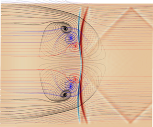
Figure 9. Streamlines evaluated in the $x{-}z$ plane at $y=1$ for the baseline $\unicode[STIX]{x1D703}_{sg}=2.0^{\circ }$ case. Streamlines are coloured by the transverse velocity component $w$ with a constant colour background. The flow diverges at saddle points (S) at the front and back of the main separation bubble. The SBLI generates strong transverse velocity gradients that cause an ejection of the corner flow towards the centreline. Streamlines within the separation bubble are directed into two foci (F) that are symmetric relative to the centreline. Two additional foci (CF) required for topological consistency are labelled in each corner region.

Figure 9 shows $u{-}w$ velocity streamlines evaluated near the bottom wall at $y=1$. Streamlines are coloured by the transverse velocity component $w$ over a constant colour background. Additional streamlines are added in the corner regions to demonstrate the ejection of the corner flow into the central separation. Streamlines are deflected at $x=150$ as the corner profile thickens, with strong transverse velocity directing the flow towards the centreline on either side. At $x=300$, the streamlines diverge between the saddle point (S) on the reattachment line and the focus (F) within the separation. Flow ejected from the corner spirals into the tornado vortex at each focus, is lifted up from the surface and transported downstream. At the front of the bubble a well-defined saddle point (S) is observed; a single streamline is seen entering the saddle point laterally along the separation line from both sides, indicating the presence of a surface lifting off the wall. Streamlines adjacent to the separating line are deflected hyperbolically into one of the foci. The pattern is similar to the ‘owl-like’ separations of the first kind introduced by Perry & Hornung (Reference Perry and Hornung1984) as shown in figure 10. There is a noticeable bulge in the reattachment line as the saddle point is shifted downstream at the centre of the span. The shift of the saddle point was less pronounced for the weaker interactions simulated in § 5.2, which were observed to have a reattachment line approximately perpendicular to the downstream flow. We also note the presence of two additional foci located in the near-wall corner region denoted as CF in figure 9. These satisfy the topological rule that, for a given surface, the number of nodes (nodal points or foci) must exceed the number of saddle points by two (Tobak & Peake Reference Tobak and Peake1982). Downstream of the central circulation, the attached flow follows a smooth laminar profile with streamlines remaining mostly parallel to each other.

Figure 10. Schematic of the ‘owl-like’ separation of the first kind adapted from Colliss et al. (Reference Colliss, Babinsky, Nübler and Lutz2016), based on the work of Perry & Hornung (Reference Perry and Hornung1984). The front saddle point (S) acts as a separating line at the start of the separation bubble. A focus (F) either side of the centreline signifies a tornado-like vortex that lifts fluid away from the surface.

Figure 11. Velocity streamlines for the baseline $\unicode[STIX]{x1D703}_{sg}=2.0^{\circ }$ case in $x{-}z$ planes above the bottom wall, at increasing heights of (black) $y=1$, (blue) $y=2$ and (red) $y=3$. Contours of dilatation rate $(\unicode[STIX]{x1D735}\boldsymbol{\cdot }\bar{u})$ are overlaid in the plane $y=7$, to show the relative position of the main shock wave and expansion fan. Negative dilatation shown in blue corresponds to the strongest regions of the incident shock. A pair of weaker transverse shock waves are seen to emanate from the interaction region and reflect off the sidewall boundary layers.

Figure 11 shows the $u{-}w$ streamline patterns at three increasing heights within the separation bubble: (black) $y=1$, (blue) $y=2$ and (red) $y=3$. A slice of dilatation rate $(\unicode[STIX]{x1D735}\boldsymbol{\cdot }\bar{u})$ is overlaid in the $y=7$ plane above the central separation bubble to show the relative position of the shock reflection. Recalling that negative (blue) and positive (red) regions of dilatation are associated with shock waves and expansions, respectively, (Johnsen et al. Reference Johnsen, Larsson, Bhagatwala, Cabot, Moin, Olson, Rawat, Shankar, Sjögreen and Yee2010), the imprint of the shock reflection is observed in this plane at $x=305$. There is a notable curving of the shock due to confinement that is consistent with figure 10(a) of the turbulent study by Wang et al. (Reference Wang, Sandham, Hu and Liu2015), despite the differences in flow conditions and boundary-layer state. The shock deforms downstream at the centreline, which is also seen to be the strongest part of the incident shock. Away from the centre, the incident shock decreases in strength, consistent with the conditions needed to produce regions of attached flow bordering the central separation bubble. Transverse shock structures discussed later in this section are observed to reflect from the sidewall boundary layers at $x=390$.

While the near-wall streamlines of figure 9 appear consistent to the schematic shown in figure 10, which is often quoted in literature for confined SBLI (Xiang & Babinsky Reference Xiang and Babinsky2019), the expanded view of figure 11 in this study shows that the foci converge towards each other on the centreline. It is plausible that the vortices from the foci weaken and reconnect on the centreline, but we were unable to clearly detect this from streamline patterns. An alternative view of the topology was proposed in figure 7(d) of Gaitonde (Reference Gaitonde2015), in which the vortex from the two foci traverses the span at a given streamwise location. Extensive efforts were made in this study to identify a focus on the symmetry plane as in figure 7(d) of Gaitonde (Reference Gaitonde2015), but none was observed. It is entirely possible that topological differences exist compared to turbulent duct SBLI, with the steady laminar problem forming a special set of solutions. The ‘owl-like’ schematic in figure 10 that shows the presence of two streamwise vortices propagating downstream has also been used to describe cases such as flow separation behind an obstacle (Colliss et al. Reference Colliss, Babinsky, Nübler and Lutz2016) where an impinging SBLI is not present. For the baseline SBLI case, we were unable to detect streamwise vortices downstream of the interaction. This could be due to the SBLI expansion at the apex of the separation bubble that directs the flow downwards towards the wall.

Figure 12. Numerical schlieren of density gradient $\log _{10}((\unicode[STIX]{x1D735}\unicode[STIX]{x1D70C})^{2})$ showing the complex shock structure downstream of the three-dimensional SBLI at $AR=1$. Three intersecting slices are shown at $x=550$, $y=15$ and $z=15$. Notable features include: (A) Compression waves from the initial sidewall boundary-layer development. (B) Main incident shock. (C) Compression waves from the start of the central separation. (D) Two conical shocks from the corner of the shock generator. (E) Expansion fan formed from the reflection of the incident shock. (F) Trailing edge expansion fan. (G) First crossing point of the reflected conical shocks. (H) Secondary reflection of the central compression waves. The four coloured markers refer to the streamwise locations of the four cross-sectional slices shown in figure 13.

Computing the logarithm of density gradient magnitudes $\text{log}_{10}((\unicode[STIX]{x1D735}\unicode[STIX]{x1D70C})^{2})$ is an effective way of numerically detecting shock structures, providing a more sensitive version of the schlieren photography techniques found in experiments. Figure 12 shows a numerical schlieren of three intersecting orthogonal slices evaluated at $x=550$, $y=15$ and $z=15$. The main shock structures are identified as follows: (A) weak compression waves from the initial development of the imposed boundary-layer profile, coalescing into weak intersecting shocks. (B) The trace of the incident swept shock through the $z=15$ plane with curvature visible at $y=15$. (C) Reflected compression wave caused by the thickened boundary layer at the base of the SBLI. (D) Reflections of the conical shocks generated at the corner of the sidewalls and shock generator ramp, discussed in more detail later in this section. (E) Expansion fan developing as the flow turns over the apex of the separation bubble. (F) The trailing expansion fan generated at $x=x_{sg}+L_{sg}$. (G) Crossing of the conical shocks after reflection from the sidewalls. The crossing point is the visible kink at $x=500$ in the $C_{f}$ plot of figure 7(a) (solid line). (H) A secondary reflection of the compression wave (C) as it reaches the upper boundary layer. Although there is a subtle shading upstream of the incident shock in the $y$ plane, we do not identify significant corner shocks as suggested by Xiang & Babinsky (Reference Xiang and Babinsky2019) for a stronger turbulent interaction. This may be due to the turbulent boundary layer in the experiments, but we note that such corner shocks were also not clearly visible in Wang et al. (Reference Wang, Sandham, Hu and Liu2015). We highlight that even the compression waves resulting from the streamline curvature caused by boundary-layer development at (A) are more prominent than the corner compression. By far the strongest structures seen downstream of the SBLI are the reflecting conical shocks of (D) and (G), consistent with the turbulent case of Wang et al. (Reference Wang, Sandham, Hu and Liu2015).

Figure 13. Numerical schlieren density gradient $\text{log}_{10}((\unicode[STIX]{x1D735}\unicode[STIX]{x1D70C})^{2})$ showing the streamwise development of the conical swept SBLI. Here $y{-}z$ slices are displayed at streamwise locations (a) $x=225$, (b) $x=275$, (c) $x=325$ and (d) $x=375$. The slice locations along the length of the duct in (a–d) are marked in red, blue, green and yellow, respectively, in figure 13. Two conical shocks generated by the initial swept SBLI in the upper left and right corner cross through each other in (a) and (b) before reflecting off the bottom wall and opposite sidewall in (c) and (d). The dark horizontal line in (a) and (b) is the main incident shock, while in (c) and (d) it is the expansion after the interaction. The start of the trailing edge expansion fan can also be seen in the upper region of (d).

The role of the reflected conical shocks (D) is clearer to see when looking at the $y{-}z$ slices at different $x$ locations in figure 13. The slices show the same numerical schlieren as before, this time located at $x=(225,275,325,375)$ in (a–d). The conical shocks are generated in the upper left and right corners of the plane at the intersections between the shock generator ramp and the two sidewalls. Stepping forward in $x$ along the duct, the conical shocks expand outwards from their starting location. In figure 13(a) and (b) the conical shocks are seen to intersect each other and continue towards the opposite sidewall. The thin dark line is the $y{-}z$ projection of the incident shock which is attached to the conical shock fronts. At the edges of (a) and (b), we see that the boundary layer has thickened as a result of the swept SBLI. Figure 13(c,d) shows the impact of the conical shocks on the opposite wall to that which they originated, as well as a dark horizontal line marking the expansion above the apex of the main separation bubble. The upper and lower portions of the shock front reflect first in (c) and can be seen to be propagate back towards their starting sidewall in (d). Comparing these slices again to the $x=550$ end slice of figure 12, we can see that the conical shocks trace a path across the span and reach their original sidewall near the outlet.

The slice in figure 13(d) also shows the start of the trailing edge expansion fan generated on the upper surface at $x_{sg}+L_{sg}=345$. An extensive search was performed using various forms of density gradients, pressure and dilatation, but no obvious corner compressions were observed near the bottom of the duct. It is possible that there are fundamental differences between simulation and experiment causing the discrepancy, or that the laminar interaction is simply too weak to generate strong corner compressions. Many experimental configurations also feature gaps between the sidewall and the shock generator, which would lead to a weakened swept SBLI effect compared to enclosed ducts. For the present work, the dominant structures crossing the centreline originate from the conical shocks generated between the upper ramp and sidewalls.

5.1 The effect of duct aspect ratio

The aim of this section is to determine how laminar SBLI are affected by a varying degree of flow confinement for the selection of narrow and wide duct configurations given in table 1. For each case, the upstream flow conditions and shock strength are held constant to the $\unicode[STIX]{x1D703}_{sg}=2^{\circ }$ one-to-one aspect ratio baseline case in the previous section. Aspect ratios ranging from one-quarter to four are considered, with the largest aspect ratio expected to show strong two-dimensional behaviour on the centreline. By comparing the span-periodic result to the larger aspect ratios, an estimation can be made of how wide a duct must be before span-periodicity is a valid assumption. The narrow aspect ratio cases will assess whether the observed strengthening of the SBLI due to sidewalls continues in the presence of even stronger flow confinement. It is important to note here that the current study focuses on the influence of a variable duct width $L_{z}$, for a constant inlet boundary-layer thickness $\unicode[STIX]{x1D6FF}_{0}^{\ast }$. The ratio of boundary-layer thickness to the scale of the duct may also be an important consideration (Benek, Suchyta & Babinsky Reference Benek, Suchyta and Babinsky2013, Reference Benek, Suchyta and Babinsky2016). While the ratio of $\unicode[STIX]{x1D6FF}_{0}^{\ast }/L_{z}$ is being varied in the present study, the constant duct height results in a fixed ratio of $\unicode[STIX]{x1D6FF}_{0}^{\ast }/L_{y}$.

Figure 14 shows the centreline skin friction along the bottom wall for (a) narrow and (b) wide aspect ratios. In each of the two plots, the solid line represents the one-to-one aspect ratio case from figure 7(a). For the narrow ducts in figure 14(a), a severe reduction in central separation length is seen and the separation point has noticeably been shifted upstream. For an aspect ratio of $AR=0.25$, the flow is almost entirely attached; the separation bubble from the initial SBLI covers only 5 % of the streamwise duct length. At $AR=0.5$, the expected asymmetric double-trough profile of a laminar separation bubble (Katzer Reference Katzer1989) is also not seen since the flow abruptly reattaches at the back of the separation bubble. The most notable features of the narrower aspect ratios are the multiple peaks in skin friction downstream of the initial interaction. These correspond to the successive crossings of the incident swept-interaction that was highlighted in figure 12. As the width of the duct has been reduced, the waves reflecting between the sidewalls have less distance to travel and cross the centreline multiple times before reaching the outlet. Rather than a further strengthening of the interaction, aspect ratios below unity are seen to suppress the interaction and exhibit shock train that traverse the span of the domain.

Figure 14. The effect of varying aspect ratio on the centreline bottom wall skin friction in the case of (a) narrowing and (b) widening aspect ratios. In each case, the skin friction is compared to the one-to-one aspect ratio baseline duct (solid line).

Table 4. The effect of aspect ratio on the baseline $\unicode[STIX]{x1D703}_{sg}=2^{\circ }$ shock generator case. Comparison is also made to a span-periodic simulation without sidewalls, demonstrating the strengthened three-dimensional interaction. Separation length is shown as a percentage of the one-to-one aspect ratio sidewall case. Here $L_{sep}$ is the separation length along the centreline and $L_{f}$ is the distance between the foci and the sidewalls.

More regular behaviour is found for the larger aspect ratios in figure 14(b), in which the three-dimensionality of the sidewall flow has less of an impact on the centreline dynamics. Consistent with the narrower cases, an increase in aspect ratio causes a downstream shift of the separation point. The same is not true for the reattachment location, however, with the widest $AR=4$ case reattaching before $AR=2$. The kink in $C_{f}$ at $x=500$ for $AR=1$, due to crossing of the sidewall reflections, is not seen for larger aspect ratios; the wider span results in the crossing occurring downstream of the computational domain. Table 4 shows the strong dependence of aspect ratio on the centreline SBLI. The third column gives the separation and reattachment locations for each of the aspect ratios. As seen in figure 14, the downstream shift of the separation location is a consistent trend each time the aspect ratio is widened, with the largest $AR=4$ case still farther downstream than for an infinite span. For the $AR=1$ and $AR=2$ cases the centreline $L_{sep}$ differs by only 1 %, despite the downstream shift of the interaction at the higher aspect ratio. At the two smallest aspect ratios, the separation length was reduced to 21 % and 74 % of the $AR=1$ result. Above $AR=2$, the bubble decreases in size as three-dimensional effects become less important to the central flow. Figure 15(a) shows a comparison of the widest duct with sidewalls to an infinite span. The shape of the skin-friction distribution agrees well at an aspect ratio of four, although $L_{sep}$ is still 9 % longer than for the idealised infinite span. The extent to which the corner interaction affects the centreline flow is of interest when assessing the viability of the infinite span assumption for modelling SBLI.

Figure 15. (a) Centreline skin friction comparison of the $AR=4$ wide duct with sidewalls to an infinite span. (b) Velocity streamline pattern above the bottom wall for the $AR=4$ duct, coloured by pressure. Half of the span is shown, $z=[0,350]$, due to the centreline symmetry.

Figure 15(b) shows velocity streamlines coloured by pressure above the bottom wall. Half of the span is displayed, as the flow is symmetric about the centreline. The near wall structures are similar to those seen for the narrower aspect ratio in figure 8(a); an attached region of flow is turned inwards by the swept shock and feeds into the central separation bubble. Foci are seen in the corner and at the edge of the central separation, but they are not as pronounced as in the $AR=1$ case. The bubble is longest in the streamwise direction at roughly 20 % of the span away from the sidewall. Separation length then reduces to a constant value at $z\approx 200$, which is maintained as the flow becomes two-dimensional towards the centreline. Beyond this point, the streamlines are seen to be antiparallel to the oncoming flow. The sidewall influence causes visible deflection of the streamlines over almost 30 % of the span, which would explain the strong dependence of aspect ratio on $L_{sep}$ for $AR=2$ and narrower. For example, at $AR=2$, the centreline is located at $z=175$, within the range of influence seen here. These results are consistent with the experimental laminar SBLI of Degrez et al. (Reference Degrez, Boccadoro and Wendt1987), in which an aspect ratio of at least 2.5 was required to see two-dimensional behaviour of the interaction.

Figure 16(a) compares the effect of aspect ratio on the streamwise separation length $L_{sep}$ and the lateral distance in $z$ between the foci and the sidewall $L_{f}$. Similar trends are found to those in the experimental literature (Babinsky, Oorebeek & Cottingham Reference Babinsky, Oorebeek and Cottingham2013; Xiang & Babinsky Reference Xiang and Babinsky2019); smaller aspect ratios lead to suppression of the central separation compared to the quasi-2-D result denoted by the dashed line. At medium aspect ratios, a peak occurs that is in good agreement to figure 11 of Babinsky et al. (Reference Babinsky, Oorebeek and Cottingham2013) and asymptotes towards the quasi-2-D result at the largest aspect ratio. The distance of the foci from the sidewall $L_{f}$ increases with aspect ratio, noting that at the smallest aspect ratio of $AR=0.25$ a clear focus could not be identified. The distance the foci shift is small relative to the width of the duct. Increasing the aspect ratio from one to four led to an increase of only 16.5 % in $L_{f}$, suggesting that the ejection of the corner flow remains mostly localised to the sides of the duct at large aspect ratios.

Figure 16. (a) The effect of duct aspect ratio on centreline streamwise separation length $L_{sep}$ and the distance between the foci and sidewalls $L_{f}$. The dashed horizontal line denotes $L_{sep}$ for the span-periodic case. (b) Normalised pressure on the sidewall ($z=0$) at increasing $y$ heights above the interaction. The ‘CS’ marker is the start of corner separation near the bottom wall.

A method for predicting the central separation size in duct SBLI was proposed by the experimental turbulent studies of Babinsky et al. (Reference Babinsky, Oorebeek and Cottingham2013), Xiang & Babinsky (Reference Xiang and Babinsky2019). The key criteria was proposed to be the streamwise crossing location of shock waves generated at the onset of corner separation. Corner shocks crossing upstream of the central interaction led to a weakened SBLI compared to quasi-2-D predictions. For shocks crossing within the interaction, a strengthened SBLI and larger separation bubble were observed. At larger aspect ratios, the flow was two-dimensional on the centreline, as the shocks crossed far downstream of the interaction. Figure 17(a) shows pressure contours for the $AR=2$ case in the present study at a height of $y=7$. This height corresponds to the apex of the central separation bubble, with the imprint of the incident shock seen at $x=300$ in this plane. The solid black line represents the $C_{f}=0$ crossing on the bottom wall of the domain ($y=0$), to serve as a reference point for the separation bubble. Two oblique structures are seen to traverse the span and cross at the back of the central interaction. As the $AR=2$ case has the largest recorded $L_{sep}$, this crossing is consistent with the trends noted in the experimental work. The same experimental trends were observed for the other aspect ratios in this work (not shown), with the smaller aspect ratio cases having structures that crossed upstream of the interaction.

Figure 17. Slices of $x{-}z$ pressure for the $AR=2$ case at (a) $y=7$ above the separation bubble and at (b) $y=70$, corresponding to 40 % of the duct height above the bottom wall. In both cases, the black line is the zero crossing of skin friction on the bottom wall ($y=0$). The crossing shocks are observed to be generated by sidewall compressions from the initial swept SBLI, independent of the onset of corner separation near the bottom wall.

Experimental work has attributed these crossing shock waves to a bottom wall corner compression effect. However, in the present simulations, observing pressure contours higher up in the duct at $y=70$ as in figure 17(b), they are seen to originate from the swept SBLI of the incident shock with the sidewalls. It is important to note that the sidewall compressions leading to the crossing shock waves occur at an earlier upstream location than the onset of bottom wall corner separation. At $x=205$, the two conical shocks interact with the incident shock and cause it to strengthen, consistent in shape with figure 9 of Wang et al. (Reference Wang, Sandham, Hu and Liu2015). The streamwise development of pressure on the sidewall is given at four $y$ heights in figure 16(b), relative to the start of the corner separation (CS). While there is a pressure rise close to the onset of corner separation at $y=7$, this effect is also present all the way up the height of the duct due to the swept SBLI and occurs upstream of the corner separation.

This section has reaffirmed that aspect ratio is a crucial parameter for confined SBLI, highlighting that span-periodicity is not a suitable assumption for internally confined flows even for relatively wide ($AR=2$) ducts. The flow at $AR=4$ still showed small differences compared to span-periodic predictions. The general impact of aspect ratio on central separation length agreed well with experimental findings. We were, however, unable to attribute this effect to the crossing of shocks from bottom wall corner compressions. It was shown that for the present study the origin of the crossing shock waves was the initial swept conical SBLI as previously identified in figure 13. This effect was shown to occur at a height above the influence of bottom wall corner compressions, and substantially further upstream than any corner separations. As a result, the crossing location is dependent on the height $y$. There are several differences in this study to the experimental work, which could be causing the difficulty in identifying strong corner shocks. The present study is laminar and far weaker ($\unicode[STIX]{x1D703}_{sg}=2^{\circ }$ versus $\unicode[STIX]{x1D703}_{sg}=8^{\circ }$), plus there is no gap between the shock generator and the sidewalls, which would emphasise the swept conical SBLI relative to weak corner compressions. Nevertheless, the present results are consistent with previous LES (Wang et al. Reference Wang, Sandham, Hu and Liu2015) of turbulent interactions with sidewalls.

5.2 Variation of incident shock strength

In this section, the initial flow deflection $\unicode[STIX]{x1D703}_{sg}$ is modified to determine the sensitivity of the SBLI to variations in incident shock strength. For each case, the starting location of the shock generator $x_{sg}$ is modified to maintain the same value of $Re_{x}$ at the inviscid impingement location. One stronger and three weaker interactions are considered for this section, corresponding to flow deflections of $\unicode[STIX]{x1D703}_{sg}=[0.5,1,1.5,2.5]$. Details of mesh convergence for the $\unicode[STIX]{x1D703}_{sg}=2.5^{\circ }$ case are discussed later in this section. Figure 18(a) shows the normalised centreline pressure along the bottom wall for the baseline and three weaker interactions. As the interaction is weakened, the pressure rise at the start of separation shifts downstream. The outlet pressure ratio $p_{3}/p_{1}$ for the three weaker interactions is given in table 5. For each shock strength, there is a lack of a pressure plateau in the middle interaction, often seen in quasi-2-D laminar SBLI (Katzer Reference Katzer1989; Sansica et al. Reference Sansica, Sandham and Hu2013). Instead, the flow reattaches quickly and for the two weakest interactions there is actually a pressure reduction after the initial compression.

Figure 18. Sensitivity of the centreline (a) wall pressure and (b) skin friction to incident shock strength for the $AR=1$ duct. The solid line represents the baseline configuration.

Table 5. Reduction in streamwise separation length $L_{sep}$ of the main interaction with decreasing incident shock strength. Comparison is made to the centreline skin friction for the baseline $\unicode[STIX]{x1D703}_{sg}=2.0^{\circ }$ case with $AR=1$.

The effect of the weakened shock on the central separation is shown in figure 18(b). Both the separation and reattachment locations shift down and upstream, respectively, for the weaker interactions, with the $\unicode[STIX]{x1D703}_{sg}=0.5^{\circ }$ case being close to incipient separation on the centreline. It was observed during the simulations that the corner region was the first to separate, owing to the large regions of low-momentum fluid in the corners. The crossing at $x=500$ of the reflected conical shocks identified in § 4.2 is less obvious for the weaker interactions. Aside from the baseline case, only the $\unicode[STIX]{x1D703}_{sg}=1.5^{\circ }$ case shows the asymmetric double-trough $C_{f}$ distribution; the weaker cases reattach abruptly in a manner similar to the narrow aspect ratio ducts in figure 14(a). Table 5 shows the separation and reattachment points for each of the shock strengths and gives the size of $L_{sep}$ relative to the baseline. Although the separation and reattachment are both sensitive to incident shock strength, the effect on the separation point is more severe. A reduction of $1.5^{\circ }$ in the initial flow deflection leads to an overall 87 % reduction in centreline separation. Each of the weaker interactions followed owl-like topologies of the first kind, with two distinct foci and saddle points. As the interaction was strengthened, there was an elongation of the separated region in the streamwise direction.

A stronger interaction at $\unicode[STIX]{x1D703}_{sg}=2.5^{\circ }$ was also performed and was found to be very close to the limits of stability downstream of the main interaction. The transition process for duct SBLI is beyond the scope of the present laminar study and will be the subject of future work. The results for the stronger interaction are included here to give insight into the limiting behaviour of large separations. A steady laminar SBLI was not obtained for the stronger interaction on the baseline grid of $(N_{x},N_{y},N_{z})=(750,455,355)$. Regions of intermittent transition were observed near the outlet. A grid refinement study was performed to determine whether the transition was due to numerical artefacts, with ${\approx}100\,\%$ additional grid points added in each direction independently. The FineX, FineY and FineZ refined grids comprised $(N_{x},N_{y},N_{z})=(1500,455,355),(750,910,355)$ and $(750,455,705)$ points, respectively. Despite the refinement, all of the simulations contained transition downstream of the SBLI and unsteadiness at the back of the separation bubble. Compared to the baseline grid, relative errors in the centreline separation length of 0.69 %, 0.19 % and 0.66 % were observed for the FineX, FineY and FineZ simulations, respectively.

Figure 19. The figure shows (a) $u{-}w$ velocity contours evaluated at $y=1$ above the bottom wall, coloured by transverse velocity component $w$. Saddle (S) and foci (F) are highlighted as in figure 9. (b) Streamwise velocity at $y=1$ above the bottom wall. The solid black line shows the $u=0$ line to highlight regions of flow-reversal. Four high-speed streaks are observed downstream of the interaction in red. A darkened imprint of the conical swept shock is also visible.

Figure 19(a) shows $u{-}w$ velocity streamlines at $y=1$ over the same range as in figure 9. The same combination of saddle points (S) and foci (F) are observed for the stronger interaction, but the size and magnitude of the separation is increased. The separation line has shifted upstream and each of the foci have been elongated in the streamwise direction relative to the weaker interaction in figure 9. The deformation of the saddle point at the reattachment line is increased; there is no longer a well-defined set of two streamlines entering the saddle point. The streamwise velocity contours of figure 19(b) show four high-speed streaks downstream of the main interaction. The central two streaks were observed to contain streamwise vorticity generation that could be an indication of the topology shown in figure 10. The flow was found to accelerate rapidly after the apex of each of the corner separations and on either side of the centreline saddle point. While the interaction is still roughly owl-like of the first kind, the deformation of the attachment line saddle point could indicate an intermediate state approaching the second owl-like state shown schematically in figure 4(a) of Eagle & Driscoll (Reference Eagle and Driscoll2014). For owl-like patterns of the second kind, the rear saddle point transitions into a node with multiple streamlines directed into it. Owl-like patterns of the second kind for turbulent SBLI have been shown to correspond to stronger interactions in experiments (Xiang & Babinsky Reference Xiang and Babinsky2019). Based on the topological trends seen in this case, it is feasible that the transition mechanism for stronger three-dimensional laminar SBLI involves the bifurcation from topologies of the first kind to the second.

5.3 The effect of the trailing expansion fan on the interaction

It was demonstrated in § 3.3 that for laminar duct SBLI the flow on the centreline is sensitive to the length of shock generator used. For longer shock generators, the trailing expansion fan recovery occurs further downstream and leads to an increase in the central separation bubble length (figure 5b). A comparison to figure 4(b) showed this is a purely 3-D effect that is not present in quasi-2-D laminar SBLI. The only difference between the quasi-2-D and 3-D simulations is the lateral confinement imposed by the sidewalls. Table 3 reported a 6 % increase in $L_{sep}$ between $L_{sg}=300$ and $L_{sg}=350$, a limiting case of maximum $L_{sep}$ was not found for the range of $L_{sg}$ tested. This section investigates the limiting behaviour of the interaction for a longer duct with both short ($L_{sg}=200$) and very long ($L_{sg}=600$) shock generators. In both cases, the trailing expansion fan is located far downstream of the central interaction and does not impinge directly on the bottom wall separation bubble. The baseline domain from table 1 is extended by ${\sim}55\,\%$ in the streamwise direction to a length of $L_{x}=850$. A grid resolution of $(1150\times 455\times 455)$ is selected with additional points in the $x$ direction, to maintain the same streamwise resolution as in the previous cases. The same laminar inflow as described in § 3.1 is used for the longer duct cases, with no random disturbances added to the inlet.

Figure 20. Long domain duct ($L_{x}=850$, $\unicode[STIX]{x1D703}_{sg}=2^{\circ }$, $AR=1$) demonstrating the ability of the trailing expansion fan to control the interaction. The figures correspond to shock generators with $L_{sg}=600$ in (a,c,e) and $L_{sg}=200$ in (b,d,f). Showing centreline density ($z=87.5$) (a,b), skin friction on the bottom wall ($y=0$) (c,d) and skin friction on the sidewall ($z=0$) (e,f). The solid white line highlights the zero crossing of skin friction, enclosing regions of flow-reversal.

Figure 20 shows the instantaneous flow features of the two long domain cases after $t=12\,000$ for shock generators of length $L_{sg}=600$ (a,c,e) and $L_{sg}=200$ (b,d,f). Instantaneous skin friction relative to the bottom ($\unicode[STIX]{x2202}u/\unicode[STIX]{x2202}y$) and sidewalls ($\unicode[STIX]{x2202}u/\unicode[STIX]{x2202}z$) are shown in (c,d) and (e,f), respectively, with centreline ($z=87.5$) density contours given in (a,b). For the skin-friction plots, the solid white line highlights the $C_{f}=0$ crossing of the component relative to that wall. In both of the density plots of figure 20(a,b), a shock train is clearly visible; compression waves at the start of the central separation coalesce into a shock that impinges on the upper surface and causes a small region of secondary flow-reversal. A further reflection occurs and this wave impinges on the bottom wall. The reflected incident shock also reflects between the upper and lower walls of the domain, highlighting the complex secondary reflections present for internally confined flows. A trailing edge expansion fan can be seen originating from the upper surface at $x=245$ for the short shock generator, first hitting the bottom wall boundary layer around $x=500$. In the long case, an expansion fan is generated at $x=645$, which exits through the outlet before hitting the bottom wall. For the long shock generator, the flow transitions to turbulence while remaining laminar for the shorter $L_{sg}=200$. This suggests that, if geometry permits, the strength and size of the central separation can be controlled by the use of shorter shock generators.

The difference in the reattached boundary-layer state is clearer to see in figure 20(c,d). For the long shock generator in figure 20(c), the flow transitions at $x=600$ on the centreline and in both corners of the duct. The corner separation is truncated as the boundary layer transitions and remains attached in the corner towards the outlet. The central separation is substantially larger for the longer shock generator and is characterised by a flat separation line across the span and a distortion of the reattachment line peaking on the centreline. The separated region covers more of the span and is also noticeably thicker in the corner regions. The shape of the interaction is very similar to the stronger $\unicode[STIX]{x1D703}_{sg}=2.5^{\circ }$ interaction shown in figure 19(b). This demonstrates that for two different methods of achieving a stronger interaction, the shape of the central separation bubble has a topology common to both. Comparing to the short shock generator of figure 20(d), we note the downstream shift of the expansion fan has led to an upstream and downstream shift of the separation and reattachment points, respectively. The downstream shift of the expansion fan in the longer case also leads to smaller secondary flow-reversal zones at $x=500$. Comparing their location to the shock pattern in figure 20(a), it is clear the secondary separations cannot be attributed to the first vertical secondary reflection that impinges at $x=600$ and instead are likely caused by the lateral reflections shown downstream of the interaction in figure 12.

Finally, the impact of shock generator length on the sidewall flow is illustrated in figure 20(e,f). While the shape of the sidewall separation is similar in both cases, the downstream shift of the trailing expansion fan leads to a significant enlargement of the sidewall flow-reversal. For the short case, it can be seen that the expansion fan causes a recovery of the sidewall flow that wards off separation after $x=400$. Smaller separation bubbles are seen further downstream due to the secondary reflections present in figure 20(b). For the long shock generator case in figure 20(e), the sidewall separation bubble covers a much larger portion of the sidewall and is only truncated as the flow begins to transition around $x=600$. As the expansion fan originates from the upper surface at $x=645$ and is directed towards the outlet, we conclude that the sidewall separation is limited by the onset of transition in the sidewall boundary layer. This is in contrast to the short shock generator case where the sidewall separation is prematurely terminated by the upstream shift of the trailing expansion fan. The importance of transition in limiting sidewall separation suggests that attempts, such as Giepman et al. (Reference Giepman, Louman, Schrijer and van Oudheusden2016), to suppress the size of laminar SBLI with transition could also benefit from placing trips on the sides of the duct. We have seen that the central separation bubble and state of the reattached boundary layer are sensitive to a shortening of the shock generator. Shorter shock generators modify the sidewall flow considerably and limit the growth of both the corner and sidewall separations. The modified interaction is observed to be weaker and leads to reduced three-dimensionality and a suppressed central separation bubble.