2 Experiments

A series of experiments were conducted to examine the effect of a salinity gradient on ice dissolution and the resulting turbulent wall plume. The experiments were carried out in a tank that was 1.2 m high, 1.5 m wide and 0.2 m long. The tank was kept in a temperature-controlled room at approximately $4\,^{\circ }\text{C}$ . Ice was grown from fresh water and then exposed to salty water. A stable salinity stratification was created using the double-bucket method described by Oster & Yanamoto (Reference Oster and Yanamoto1962). A floating polystyrene boat with a porous base was used to reduce the momentum of the input and avoid the interior fluid mixing while the tank was being filled. During filling the ice was protected from the salty water by an acrylic barrier. The experimental apparatus and method are more fully described in Kerr & McConnochie (Reference Kerr and McConnochie2015).

All of the experiments were conducted with a mean far-field salinity of $3.5\pm 0.2~\text{wt}\%~\text{NaCl}$ and an ambient temperature of $3.5\pm 0.2\,^{\circ }\text{C}$ . Using the double-bucket method we produced density gradients between $\text{d}{\it\rho}/\text{d}z=0.04~\text{kg}~\text{m}^{-4}$ and $\text{d}{\it\rho}/\text{d}z=9~\text{kg}~\text{m}^{-4}$ . Stronger gradients were avoided as they would have resulted in a significant section of the wall plume being laminar. Turbulence could have been enhanced in the plume by increasing the far-field salinity or temperature, but this was avoided to simplify the comparison with icebergs and ice shelves in the polar oceans.

The salinity gradient was measured with a conductivity–temperature probe that traversed vertically through the far field. At the start of each experiment it was calibrated against standard salinity solutions. A traverse was conducted at the start of the experiment to measure the initial salinity gradient.

During an experiment, a cold and fresh meltwater layer propagated downward through the tank. The interface between this meltwater layer and the unmodified ambient fluid below will hereafter be referred to as the first front. Conductivity–temperature traverses were performed every 20 min to measure the propagation of the first front during an experiment (McConnochie & Kerr Reference McConnochie and Kerr2016). All measurements of interface temperature, ablation velocity and plume velocity were made below the first front where the far-field temperature and salinity were constant to within $0.2\,^{\circ }\text{C}$ and $0.2~\text{wt}\%~\text{NaCl}$ respectively. Measurements of plume velocity and most measurements of ablation velocity were made in the early stages of an experiment where the changes in far-field conditions were significantly smaller.

Temperatures within the ice and the plume were measured throughout each experiment using thermistors at heights of approximately 32, 42, 56 and 70 cm from the base of the tank. As the ice retreated, they recorded the temperature through the ice, at the ice–water interface and through the turbulent wall plume. The ice–water interface was identified as the point where the temperature gradient suddenly increased. It could also be identified as the location immediately before the large temperature fluctuations caused by turbulence in the wall plume. Measurements of interface temperature were constant with time and height to within $0.1\,^{\circ }\text{C}$ . An example of a typical thermistor log is shown in figure 1. In figure 1 the temperature is seen to slowly decrease after approximately 80 min. This decreasing temperature reflects the downward propagation of the first front throughout an experiment.

Figure 1. A characteristic thermistor log from a thermistor initially frozen into the ice, $70~\text{cm}$ above the base of the tank. In this experiment the far-field temperature was $3.5\,^{\circ }\text{C}$ , the mean far-field salinity was $3.55~\text{wt}\%~\text{NaCl}$ and the Brunt–Väisälä frequency was $0.06~\text{rad}~\text{s}^{-1}$ . The recorded interface temperature from this experiment is $-0.58\,^{\circ }\text{C}$ , which corresponds to approximately 10 min on this particular thermistor log.

Figure 2. A series of shadowgraph images showing the ice on the right-hand side of each image and the ambient salt water on the left. The rising wall plume is visible between the ice and the still ambient fluid. These photographs were taken from a qualitative experiment with a far-field temperature of $3.4\,^{\circ }\text{C}$ , a mean far-field salinity of $3.55~\text{wt}\%~\text{NaCl}$ and a Brunt–Väisälä frequency of $0.21~\text{rad}~\text{s}^{-1}$ after approximately 2 h. The scale on the left of each image shows the height in centimetres from the base of the tank; (a) shows the ice from the base of the tank to a height of 27 cm, and (b–d) show heights of 18–49, 44–76 and 74 cm to the surface of the fluid at 105 cm. A transition from laminar to turbulent flow in the wall plume can also be observed at approximately $19~\text{cm}$ from the base of the tank. Intruding double-diffusive layers can be observed in the upper two sections.

The experiments were visualised using the shadowgraph method and recorded with photographs from a Nikon D100 DSLR camera. A series of shadowgraph images from a typical experiment are shown in figure 2. Double-diffusive layers are clearly visible in figure 2, particularly in figure 2(c,d). Double-diffusive layers were typically observed in the experiments despite the majority of plume fluid appearing to rise to the top of the tank. In the more strongly stratified experiments more fluid seemed to detrain into each layer and the double-diffusive layers were more visible. In the experiment shown in figure 2 a large fraction of the meltwater detrained into the double-diffusive layers. As a result, the first front was approximately 6 cm from the water surface when the photographs were taken.

In general, the layer scale was uniform and as predicted by (1.1). We note that it would appear to be more logical to use the interface temperature instead of the freezing-point temperature at the mean far-field salinity in (1.1). However, due to the small thermal expansion coefficient at low temperatures, the effect on the predicted layer scale is only 6 %.

The ablation velocity was calculated by comparing the position of the ice–water interface in photos taken 30 min apart. This method gave continuous ablation profiles up the height of the ice, averaged over a 30 min period. Two consecutive 30 min periods were compared to ensure that the ablation velocity was constant with time. The two periods gave ablation velocities that agreed to within $0.1~{\rm\mu}\text{m}~\text{s}^{-1}$ . The quoted values are the averages of these two 30 min time periods. It is estimated that measurements of the ablation velocity had an error of approximately $0.1~{\rm\mu}\text{m}~\text{s}^{-1}$ based on the resolution of the images and comparison of the two time periods.

The maximum plume velocity was measured to within 5 % using the shadowgraph particle tracking velocimetry (shadowgraph PTV) technique described in McConnochie & Kerr (Reference McConnochie and Kerr2016). Shadowgraph PTV is an adaptation of traditional PTV where turbulent eddies are tracked instead of particles. Jonassen, Settles & Tronosky (Reference Jonassen, Settles and Tronosky2006) used a very similar technique for investigating the velocity structure in a variety of turbulent flows. The PTV software ‘Streams’ (Nokes Reference Nokes2014) was used for feature identification, particle matching and the computation of velocity fields. For very strongly stratified experiments, there were insufficient turbulent eddies, and the eddies that did exist were not persistent enough to be suitable for tracking. This provided an upper limit on the strength of stratification that we investigated. However, our experiments at weaker stratifications were sufficient to determine the effect of stratification on the maximum plume velocity.

3 Interface conditions

3.1 Interface temperature

Table 1 shows the experimental parameters and results for the stratified ambient experiments where an interface temperature was measured. Like the homogeneous ambient experiments of Kerr & McConnochie (Reference Kerr and McConnochie2015), we observed no height dependence on interface temperature.

Figure 3 shows the measured interface temperature as a function of the Brunt–Väisälä frequency, $N=(-(g/{\it\rho}_{0})(\text{d}{\it\rho}/\text{d}z))^{1/2}$ , where ${\it\rho}_{0}$ is the density at mid-depth. The theory of Kerr & McConnochie (Reference Kerr and McConnochie2015) suggests that, for a far-field temperature of $T_{f}=3.5\,^{\circ }\text{C}$ and a homogeneous far-field salinity of $C_{f}=3.5~\text{wt}\%~\text{NaCl}$ , the interface temperature should be $-0.52\,^{\circ }\text{C}$ . This agrees with the low-stratification experiments shown in figure 3.

Figure 3. The measured interface temperature as a function of the Brunt–Väisälä frequency. The measurements had a typical uncertainty of $0.1\,^{\circ }\text{C}$ . Different symbols relate to different values of $T_{f}$ , with $\times$  relating to $T_{f}=3.3\,^{\circ }\text{C}$ , ♢ to $T_{f}=3.4\,^{\circ }\text{C}$ , ○ to $T_{f}=3.5\,^{\circ }\text{C}$ , ▫ to $T_{f}=3.6\,^{\circ }\text{C}$ and ▵ to $T_{f}=3.7\,^{\circ }\text{C}$ . The inset shows the five experiments around $N=0.08~\text{rad}~\text{s}^{-1}$ . The data point at $N=0$ , $T_{i}=-0.52$ agrees to within $0.01\,^{\circ }\text{C}$ with the prediction of Kerr & McConnochie (Reference Kerr and McConnochie2015). The interface temperature is clearly reduced by a salinity gradient. The liquidus temperature at the far-field salinity is approximately $-2.1\,^{\circ }\text{C}$ , which shows that the interface salinity is still much less than the far-field salinity at the apparent high-stratification limit.

Table 1. The measured interface temperature $T_{i}$ , with the Brunt–Väisälä frequency $N$ , the far-field temperature $T_{f}$ and the mean far-field salinity $C_{f}$ . The interface salinity $C_{i}$ is calculated from a linear approximation of the liquidus relationship, $C_{i}=-1.686~T_{i}$ , based on the data in Weast (Reference Weast1989). We note that in some cases the far-field salinity and Brunt–Väisälä frequency were measured using density samples as the conductivity–temperature traverser was yet to be installed. This is reflected by the less accurately measured Brunt–Väisälä frequency in some experiments.

However, as the stratification increases the interface temperature is seen to be reduced. There appears to exist an upper limit beyond which stratification will not continue to reduce the interface temperature. This high-stratification limit is significantly above the liquidus temperature of the far field, which is approximately $-2.1\,^{\circ }\text{C}$ . The apparent lower limit on interface temperature from our experiments is $-1.4\,^{\circ }\text{C}$ , which suggests an upper limit on interface salinity of approximately $2.4~\text{wt}\%~\text{NaCl}$ .

3.2 Ablation velocity

Figure 4 shows the ablation velocity up the ice wall for six different experiments. Five of the experiments were conducted in a stratified ambient fluid and one was conducted in a homogeneous ambient fluid. In all cases the far-field temperature and mean far-field salinity were approximately $3.5\,^{\circ }\text{C}$ and $3.5~\text{wt}\%~\text{NaCl}$ respectively. All profiles show a maximum ablation velocity at approximately 150–200 mm from the base of the tank. This height corresponds to the transition from laminar to turbulent flow in the wall plume, which leads to a flow of ambient water towards the ice (Josberger & Martin Reference Josberger and Martin1981). Above the turbulent transition the ablation velocity is seen to be constant in a homogeneous ambient fluid (as described in Kerr & McConnochie Reference Kerr and McConnochie2015), but it decreases with height in a stratified ambient fluid.

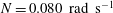
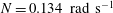
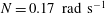
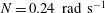
Figure 4. Ablation velocity with height for six different experiments: (a) $N=0~\text{rad}~\text{s}^{-1}$ ; (b) $N=0.036~\text{rad}~\text{ s}^{-1}$ ; (c) $N=0.080~\text{rad}~\text{s}^{-1}$ ; (d) $N=0.134~\text{rad}~\text{s}^{-1}$ ; (e) $N=0.17~\text{rad}~\text{s}^{-1}$ ; (f) $N=0.24~\text{rad}~\text{s}^{-1}$ . Unlike the homogeneous case, the stratified experiments have a decreasing ablation velocity with height. The small-scale vertical variation is not related to the double-diffusive layer scale and is a result of smoothing the experimental data.

Table 2 and figure 5 show the ablation velocity at three points on the ice for all stratified experiments. The three heights shown are defined as the bottom, middle and top of the tank, relating to 200–250, 475–525 and 750–800 mm from the base of the tank respectively. These definitions mean that the bottom region is just above the turbulent transition and the top region is below the first front. Figure 5 shows that a salinity gradient acts to reduce the ablation velocity at all heights. However, this effect appears to be more significant near the top of the tank.

Table 2. Ablation velocities at several heights for experiments with different Brunt–Väisälä frequencies, $N$ , but almost constant far-field temperature, $T_{f}$ , and mean far-field salinity, $C_{f}$ . The top refers to 750–800 mm from the base of the tank and is just below the meltwater first front. The bottom refers to 200–250 mm from the base of the tank and is immediately above the point where the wall plume becomes turbulent. The middle refers to 475–525 mm from the base of the tank and is halfway between the top and the bottom.

Figure 5. The ablation velocity as a function of the Brunt–Väisälä frequency for three different ice heights: (a) top ablation velocity, (b) middle ablation velocity, (c) bottom ablation velocity. The top refers to 750–800 mm from the base of the tank and is just below the meltwater first front. The bottom refers to 200–250 mm from the base of the tank and is immediately above the point where the wall plume becomes turbulent. The middle refers to 475–525 mm from the base of the tank and is halfway between the top and the bottom.

4 Plume properties

4.1 Plume velocity

We have performed the same analysis as McConnochie & Kerr (Reference McConnochie and Kerr2016) on the wall plume resulting from dissolving ice into a stratified salty fluid. We have assumed that the maximum velocity will still scale like a power-law function of height but allowed the specific power-law function to change with stratification. This corresponds to a maximum vertical velocity that, for almost constant far-field conditions, is described by

(4.1) $$\begin{eqnarray}w=A(N)z^{x(N)},\end{eqnarray}$$

where $A(N)$ and $x(N)$ are unknown functions of the Brunt–Väisälä frequency and $z$ is the height measured from the turbulent transition. Since the ablation velocity depends on height, the buoyancy flux will also depend on height, and the functions $A(N)$ and $x(N)$ may also depend on height. We have, however, observed no evidence for this and herewith assume that both $A$ and $x$ are height-independent.

Figure 6 shows the measured velocities as a function of height for four typical experiments. It can be seen that the power-law fits from (4.1) describe the experimental measurements to within 5 %. This suggests that the power-law assumption in (4.1) is a reasonable approximation for the plume velocity up the wall, at least in the range of experimental conditions.

Figure 6. Measured maximum vertical velocities as a function of height for four typical experiments. The power-law fits using (4.1) and table 3 are plotted with the experimental data. The power laws are seen to match the experimental data over the full range of Brunt–Väisälä frequencies.

Table 3 shows the far-field conditions and values of $x$ and $A$ for experiments over a range of experimental stratifications. The values of $A$ are calculated using the measured velocity power for each experiment. As noted in § 2, it was not possible to measure the plume velocity using shadowgraph PTV in more strongly stratified ambients as there were insufficient turbulent eddies to be tracked.

Table 3. The measured coefficients of the assumed plume velocity equation $w=Az^{x}$ for experiments with different Brunt–Väisälä frequencies, $N$ , constant far-field temperature, $T_{f}$ , and constant mean far-field salinity, $C_{f}$ . Also shown is the double-diffusive layer height, $h$ , as defined by (1.1).

Figure 7 shows the measured values of the velocity power, $x$ from (4.1), plotted against the ambient Brunt–Väisälä frequency. It can be seen that for a very weakly stratified ambient ( 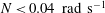$N<0.04~\text{rad}~\text{s}^{-1}$ ), stratification has no effect on the plume velocity power. However, for more strongly stratified ambient conditions the velocity power appears to be suddenly reduced. It is unclear whether the reduced velocity power is caused by the decreasing buoyancy flux with height in the stratified experiments or by the stratification affecting the plume itself. However, since the ablation velocity does not show the same dramatic change in behaviour as the velocity power it is likely that the plume is changed predominantly by the stratification and not by the non-uniform source buoyancy flux.

Figure 7. Measured values of the velocity power, $x$ in (4.1), as a function of the Brunt–Väisälä frequency.

The point where stratification appears to inhibit the plume acceleration seems to correspond well with the predicted double-diffusive layer scale being smaller than the tank height. In these experiments the fluid height was typically approximately 1.05 m. Because of this it is unlikely that any stratification with a layer scale larger than 1 m would have an impact on the plume. However, in the case of the more strongly stratified experiments with layer scales between 0.1 and 0.3 m there is sufficient height for several layers to form within the tank. In these experiments, double-diffusive layers could also be observed on the shadowgraph record. The presence of layers shows that there is significant detrainment from the plume. Detrainment will affect the plume buoyancy and potentially increase the drag on the plume. An increased drag or reduced buoyancy flux could each explain the reduced plume acceleration.

Figure 8 shows calculated values of the velocity coefficient, $A$ from (4.1). It is observed that stratification reduces the velocity coefficient as well as the velocity power. However, in the case of the velocity coefficient, the reduction occurs even at very low stratifications where the velocity power is unaffected. The velocity coefficient also decreases gradually and not in the sudden manner of the velocity power. The gradual decrease is similar to the gradual decrease in ablation velocity in the stratified experiments. Since a reduced ablation velocity will lead to a reduced buoyancy flux, (1.4) suggests that a smaller velocity coefficient can be explained by a smaller ablation velocity.

Figure 8. Calculated values of the velocity coefficient, $A$ in (4.1), as a function of the Brunt–Väisälä frequency. The velocity powers shown in table 3 and figure 7 are used to calculate the velocity coefficients for each experiment.

4.2 Plume buoyancy

In a homogeneous fluid, McConnochie & Kerr (Reference McConnochie and Kerr2016) showed that the top-hat plume buoyancy can be described by

(4.2) $$\begin{eqnarray}{\it\Delta}=(23\pm 2){\it\Phi}^{2/3}z^{-1/3},\end{eqnarray}$$

where ${\it\Delta}$ is the top-hat buoyancy in the plume at height $z$ :

(4.3) $$\begin{eqnarray}{\it\Delta}=g\left(\frac{{\it\rho}_{f}-{\it\rho}}{{\it\rho}_{f}}\right),\end{eqnarray}$$

where ${\it\rho}_{f}$ is the far-field density and ${\it\rho}$ is the plume density.

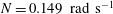
For an experiment with Brunt–Väisälä frequency $N=0.149~\text{rad}~\text{s}^{-1}$ , far-field temperature $T_{f}=3.7\,^{\circ }\text{C}$ and mean far-field salinity $C_{f}=3.6$ wt% NaCl, samples were taken from a 1 mm diameter stainless steel tube placed directly against the ice at three distinct heights. The density of these samples was measured and the buoyancy was calculated as in (4.3). Table 4 and figure 9 show the buoyancy of the plume based on the density samples.

Table 4. Measured values of the plume buoyancy, ${\it\Delta}$ , at various heights above the turbulent transition, $z$ ; ${\it\Delta}_{ave}$ is the average value at each height. The experiment had a Brunt–Väisälä frequency $N=0.149~\text{rad}~\text{s}^{-1}$ , a far-field temperature $T_{f}=3.7\,^{\circ }\text{C}$ and a mean far-field salinity $C_{f}=3.6$ wt% NaCl.

Figure 9. Measured values of the plume buoyancy for an experiment with Brunt–Väisälä frequency $N=0.149~\text{rad}~\text{s}^{-1}$ , far-field temperature $T_{f}=3.7\,^{\circ }\text{C}$ and mean far-field salinity $C_{f}=3.6$ wt% NaCl. The circles show the measured values and the triangles show the average value at each height.

It was not possible to take samples with sufficient accuracy to determine the equivalent top-hat plume buoyancy, as each sample would have been taken from a slightly different part of the plume. However, it is clear that the buoyancy in the plume is increasing with height.

This observation contrasts with the predictions of (4.2), which suggests that the buoyancy should decrease with height. For the plume buoyancy to increase with height the turbulent plume must be becoming fresher with height. It is likely that it becomes colder since heat and salt are typically linked in these experiments. A freshening plume leads to a reducing ablation velocity and may help to explain the height dependence of the ablation velocity.

5 Physical discussion and scaling

The results presented in §§ 3 and 4 show that stratification has a significant impact on both the interface and the plume conditions. However, it is important to consider how our results will scale from the laboratory to a geophysical scale. Our laboratory experiments involved approximately 1 m of ice, whereas Antarctic icebergs and ice shelves have typical keel depths of approximately 200 m and 500 m respectively (Dowdeswell & Bamber Reference Dowdeswell and Bamber2007; Jenkins et al. Reference Jenkins, Dutrieux, Mcphail, Perrett, Webb and White2010). We propose an argument for scaling the stratification to geophysical scales based on the top-hat model of turbulent wall plumes in a homogeneous fluid (Cooper & Hunt Reference Cooper and Hunt2010; McConnochie & Kerr Reference McConnochie and Kerr2016).

The plume buoyancy flux, $F$ , can be described by

(5.1) $$\begin{eqnarray}\frac{\text{d}F}{\text{d}z}={\it\Phi}_{o}-QN^{2},\end{eqnarray}$$

where $Q$ is the plume volume flux and ${\it\Phi}_{o}$ is the source buoyancy flux per unit area without stratification. When $N^{2}\sim {\it\Phi}_{o}/Q$ , stratification will become important. Since we are looking for the point where stratification first becomes important we set $N^{2}={\it\Phi}_{o}/Q$ and use $Q=0.043{\it\Phi}_{o}^{1/3}z^{4/3}$ . The equation for $Q$ was obtained by measuring the first front position during experiments conducted in a homogeneous ambient fluid (McConnochie & Kerr Reference McConnochie and Kerr2016). This gives

(5.2) $$\begin{eqnarray}N^{2}=\frac{{\it\Phi}_{o}}{Q}=\frac{{\it\Phi}_{o}}{0.043{\it\Phi}_{o}^{1/3}z^{4/3}}=23\frac{{\it\Phi}_{o}^{2/3}}{z^{4/3}}.\end{eqnarray}$$

A typical buoyancy flux from a homogeneous experiment with similar far-field conditions to our stratified experiments was ${\it\Phi}_{o}=4.6\times 10^{-7}~\text{m}^{2}~\text{s}^{-3}$ (McConnochie & Kerr Reference McConnochie and Kerr2016). Using this source buoyancy flux and a typical laboratory height of 1 m, we obtain a critical Brunt–Väisälä frequency in the laboratory of

(5.3) $$\begin{eqnarray}N_{c}=0.037~\text{rad}~\text{s}^{-1}.\end{eqnarray}$$

A critical Brunt–Väisälä frequency of approximately $0.037~\text{rad}~\text{s}^{-1}$ in the laboratory is in reasonable agreement with figures 3, 5 and 7. For weaker stratifications there is a minimal deviation from the homogeneous case, but for stronger stratifications the plume and interface conditions are significantly changed.

This critical Brunt–Väisälä frequency suggests the following scaling between the laboratory and the ocean:

(5.4) $$\begin{eqnarray}N_{lab}=N_{ocean}\left(\frac{{\it\Phi}_{o,lab}}{{\it\Phi}_{o,ocean}}\right)^{1/3}\left(\frac{z_{ocean}}{z_{lab}}\right)^{2/3}.\end{eqnarray}$$

Alternatively, a critical height, $z_{c}$ , can be calculated. Rearranging (5.2) to obtain the critical height gives

(5.5) $$\begin{eqnarray}z_{c}=11\frac{{\it\Phi}_{o}^{1/2}}{N^{3/2}}.\end{eqnarray}$$

At heights below $z_{c}$ stratification should not be important, but for heights larger than $z_{c}$ stratification will have an increasingly important effect.

Equation (5.2) can also be used to define a non-dimensional stratification parameter, $S$ , as

(5.6) $$\begin{eqnarray}S=\frac{N^{2}Q}{{\it\Phi}_{o}}.\end{eqnarray}$$

In cases where $S\leqslant 1$ , we would expect the dissolution of the ice and the resulting wall plume to be described by the homogeneous theory of Kerr & McConnochie (Reference Kerr and McConnochie2015) and McConnochie & Kerr (Reference McConnochie and Kerr2016). However, when $S$ is larger than 1, the stratification will begin to affect the flow and the homogeneous theory will become increasingly inaccurate.

6 Application of scaling

We now test the scaling developed in § 5 by applying it to our experimental results from §§ 3 and 4. The non-dimensional ablation velocity, $V^{\ast }$ , and plume velocity, $w^{\ast }$ , can be written as

(6.1) $$\begin{eqnarray}V^{\ast }=\frac{V}{Nz}\end{eqnarray}$$

and

(6.2) $$\begin{eqnarray}w^{\ast }=\frac{w}{Nz}.\end{eqnarray}$$

We also define a new stratification parameter,

(6.3) $$\begin{eqnarray}S^{\ast }=S^{-3/4}=\frac{{\it\Phi}_{o}^{3/4}}{N^{3/2}Q^{3/4}},\end{eqnarray}$$

to compare $w^{\ast }$ and $V^{\ast }$ against. Using $Q=0.043{\it\Phi}_{o}^{1/3}z^{4/3}$ from McConnochie & Kerr (Reference McConnochie and Kerr2016) gives

(6.4) $$\begin{eqnarray}S^{\ast }=\frac{{\it\Phi}_{o}^{1/2}}{10.5N^{3/2}z}.\end{eqnarray}$$

This is done so that any quantities that are height-independent will appear as straight lines in the following analysis.

Figure 10 shows the non-dimensional ablation velocity, $V^{\ast }$ , plotted against $S^{\ast }$ . The data plotted are the same as those in figure 5. The scaled data are seen to collapse towards a single curve. At low values of $N$ (high $S^{\ast }$ ) we expect the ablation velocity to be height-independent (Kerr & McConnochie Reference Kerr and McConnochie2015). This suggests that the non-dimensional ablation velocity should be proportional to $S^{\ast }$ . For high values of $S^{\ast }$ the data plotted in figure 10 are approximately linear.

Figure 10. The non-dimensional ablation velocity plotted against $S^{\ast }$ . The data plotted are the same as those plotted in figure 5.

Figure 11 shows the non-dimensional plume velocity, $w^{\ast }$ , plotted against $S^{\ast }$ . The data plotted are the same as those in figure 6. Once again, the scaled data collapse towards a single curve. At low $N$ (high $S^{\ast }$ ) we expect the plume velocity to scale like $z^{1/3}$ (Kerr & McConnochie Reference Kerr and McConnochie2015). Such a scaling suggests that the non-dimensional plume velocity should scale like $(S^{\ast })^{2/3}=S^{-1/2}$ . The solid line plotted in figure 11 shows the expected scaling for low $N$ . It is seen to be in reasonable agreement with the experimental data for approximately $S^{\ast }>5$ . For $S^{\ast }<5$ the $w^{\ast }\sim (S^{\ast })^{2/3}$ scaling becomes increasingly inaccurate. This is expected from examination of figure 7 as the velocity power, $x$ , becomes much less than $1/3$ and the assumed power-law dependence becomes less reliable. In particular, the assumption that $A$ and $x$ (from (4.1)) are simple functions of $N$ could be incorrect and both quantities could instead be functions of $S$ .

Figure 11. The non-dimensional plume velocity plotted against $S^{\ast }$ . The data plotted are the same as those plotted in figure 6. The $w^{\ast }\sim (S^{\ast })^{2/3}$ relationship expected for high values of $S^{\ast }$ is plotted by the solid curve.

The collapse of the scaled data onto a single curve suggests that the stratification parameter, as defined in (5.6), describes most of the variability observed in figures 5 and 6.

7 Oceanographic application

The scaling given in (5.4) allows us to directly compare our experiments with oceanographic observations around Antarctica and Greenland. Table 5 gives some observed values for the Brunt–Väisälä frequency near the base of various ice shelves and glaciers. The Brunt–Väisälä frequency was calculated at the deepest section of the profile, as the critical height is typically much less than the water column depth (see table 5). These have been used to calculate equivalent laboratory-scale Brunt–Väisälä frequencies that relate to the results presented in §§ 3 and 4. We also provide values for the critical height, $z_{c}$ , and stratification parameter, $S$ , for these glaciers and ice shelves. It should be noted that in our experiments the ice face was vertical, whereas ice shelves typically have sloping sides and complex geometry.

Table 5. Observed Brunt–Väisälä frequencies and heights, $H$ , from various glaciers in Antarctica and Greenland with the laboratory-equivalent Brunt–Väisälä frequency shown. The observed heights are from the oceanographic measurement closest to the ice face and do not necessarily represent the height of the ice face. Values of the critical height, $z_{c}$ , from (5.5), and the stratification parameter, $S$ , from (5.6), are also shown. For the calculation of $z_{c}$ and $S$ , a buoyancy flux of ${\it\Phi}=1.7\times 10^{-7}~\text{m}^{2}~\text{s}^{-3}$ is assumed (McConnochie & Kerr Reference McConnochie and Kerr2016). The observational data come from

a Robinson et al. (Reference Robinson, Williams, Barrett and Pyne2010).

b Rignot & Jacobs (Reference Rignot and Jacobs2002), Williams et al. (Reference Williams, Hindell, Houssais, Tamura and Field2011).

c Jenkins et al. (Reference Jenkins, Dutrieux, Mcphail, Perrett, Webb and White2010).

d Venables & Meredith (Reference Venables and Meredith2014).

e Sutherland, Straneo & Pickart (Reference Sutherland, Straneo and Pickart2014).

Based on the scaled values of $N_{lab}$ in table 5 and the experimental results in §§ 3 and 4 it is clear that stratification is expected to affect the dissolution of ice shelves in both Greenland and Antarctica. Based on the assumption that the ice dissolution is controlled primarily by convection (Kerr & McConnochie Reference Kerr and McConnochie2015), our experimental results suggest that stratification will begin to reduce the ablation velocity and interface temperature at a laboratory Brunt–Väisälä frequency of approximately $0.04~\text{rad}~\text{s}^{-1}$ . Furthermore, it is likely that a change in ocean stratification would have a significant effect on the ice–ocean interactions. As such, when considering how the Antarctic and Greenland ice sheets may respond to a changing climate, it is important to consider stratification as well as the more commonly considered mean ocean temperature and salinity.