


1. Introduction
Wall roughness has important effects on turbulent flows, especially at high Reynolds numbers. Surfaces with riblets enable drag reduction (Bechert et al. Reference Bechert, Bruse, Hage, Van der Hoeven and Hoppe1997), sediment and vegetation canopies affect the near-bed region (Mignot, Barthélemy & Hurther Reference Mignot, Barthélemy and Hurther2009) and ‘urban roughness’ influences the urban climate (Cheng & Castro Reference Cheng and Castro2002). Many processes such as erosion, pitting (Bons et al. Reference Bons, Taylor, McClain and Rivir2001) and bio-fouling (Kirschner & Brennan Reference Kirschner and Brennan2012) produce complex surface topographies, which decrease the efficiency of engineering systems. Raupach, Antonia & Rajagopalan (Reference Raupach, Antonia and Rajagopalan1991) and Jiménez (Reference Jiménez2004) have summarized the effects of roughness on turbulent boundary layers. They describe the offset of the mean velocity profile, the enhancement of turbulent intensities and the modification of flow structures. The roughness function  $\Delta U^+= \Delta U u_{\tau }/\nu$, where
  $\Delta U$ is the difference in mean velocity between smooth and rough walls in the logarithmic layer,
  $u_{\tau }$ is the average friction velocity and
  $\nu$ is the kinematic viscosity of the fluid. Based on experiments by Nikuradse (Reference Nikuradse1933) for sand-grain roughness, three flow regimes are defined for rough-wall flows by expressing
  $\Delta U^+$ as a function of
  $k^+$, the roughness scale in viscous units. When
  $k^+$ is small,
  $\Delta U^+$ is nearly zero, i.e. the flow is hydraulically smooth. In this regime, the viscosity damps out the perturbations caused by the roughness. The flow becomes transitionally rough as
  $k^+$ increases, where the skin friction has contributions from both viscous drag and form drag. As
  $k^+$ further increases, the roughness function reaches a linear asymptote, and the flow is considered fully rough.
The roughness scale is an important parameter and different definitions exist, such as the average roughness height  $k_a^+$, the peak-to-valley roughness height
  $k_t^+$ and the equivalent sand-grain roughness height
  $k_s^+$. According to Nikuradse (Reference Nikuradse1933),
  $k_s^+$ is determined by fitting a roughness height to match the measured pressure drop in experiments. Jiménez (Reference Jiménez2004) and Flack & Schultz (Reference Flack and Schultz2010) suggest that
  $k_s^+$ can provide good collapse of
  $\Delta U^+$ in the fully rough regime for various types of roughness. Correlations to predict the frictional drag for rough surfaces are summarized by Flack & Schultz (Reference Flack and Schultz2010), who also propose a new correlation to predict
  $k_s$ in the fully rough regime. However, data for
  $\Delta U^+$ in the transitionally rough regime show considerable scatter for different roughness types. Flack & Schultz (Reference Flack and Schultz2010) note that the transitionally rough regime is the least understood, and the parameter ranges that determine the transitionally rough regime remain unknown for most roughness types. Barros, Schultz & Flack (Reference Barros, Schultz and Flack2018) measured the skin friction for systematically controlled random rough surfaces and concluded that the understanding of the frictional drag in the transitionally rough regime is poor.
Surface roughness can be categorized as being regular or irregular/random. Many experimental and computational studies (Schlichting Reference Schlichting1936; Bechert et al. Reference Bechert, Bruse, Hage, Van der Hoeven and Hoppe1997; Orlandi & Leonardi Reference Orlandi and Leonardi2006; Lee, Sung & Krogstad Reference Lee, Sung and Krogstad2011) have examined the effects of regular roughness involving ribbed, cubed or spherical elements. Recently, more attention has been paid to irregular rough surfaces (Mejia-Alvarez & Christensen Reference Mejia-Alvarez and Christensen2010; Cardillo et al. Reference Cardillo, Chen, Araya, Newman, Jansen and Castillo2013; Yuan & Piomelli Reference Yuan and Piomelli2014; Anderson et al. Reference Anderson, Barros, Christensen and Awasthi2015; Busse, Lützner & Sandham Reference Busse, Lützner and Sandham2015). The effects of irregular roughness on velocity profiles, turbulent intensities, turbulent kinetic energy and two-point correlations have been examined. Flack, Schultz & Shapiro (Reference Flack, Schultz and Shapiro2005) and Wu & Christensen (Reference Wu and Christensen2007) found that for small roughness heights (relative to the boundary layer thickness or channel half-height), ‘outer-layer similarity’ (Townsend Reference Townsend1980) holds and turbulent statistics in the outer layer are not directly affected by the roughness. The near-wall region where the roughness effects on the mean flow are significant is termed the ‘roughness sublayer’. Busse, Thakkar & Sandham (Reference Busse, Thakkar and Sandham2017) investigated  $Re$ dependence of the near-wall flow in the vicinity of and within rough surfaces. They characterized the near-wall flow by estimating the thickness of the roughness sublayer and examining the probability distribution of the reverse flow. Jelly & Busse (Reference Jelly and Busse2018) studied the dependence of the near-wall flow on higher-order surface parameters, such as skewness, by evaluating the influence on the roughness function.
Rough surfaces produce statistically inhomogeneous flow fields in the roughness sublayer on the length scale of the roughness. The multiple length scales present in random rough surfaces can cause the inhomogeneity to be quite complex. The ‘double-averaging’ (DA) decomposition, first introduced by Raupach & Shaw (Reference Raupach and Shaw1982) to examine the ‘wake production’ term within vegetation canopies, is used to describe this spatial inhomogeneity in the time-averaged flow field. Section 3.2 describes the DA decomposition as used in the present work. While standard Reynolds-averaging yields the Reynolds stress, the DA decomposition yields a ‘dispersive stress’ which represents the contribution of spatially correlated time-averaged flow to momentum transport. Dispersive stresses for regular roughness were studied by Cheng & Castro (Reference Cheng and Castro2002), Coceal, Thomas & Belcher (Reference Coceal, Thomas and Belcher2007) and Bailey & Stoll (Reference Bailey and Stoll2013). The ratio of maximum dispersive stress to Reynolds stress was found by Forooghi et al. (Reference Forooghi, Stroh, Schlatter and Frohnapfel2018) to be highly dependent on the skewness and effective slope, for irregular rough surfaces. Yuan & Jouybari (Reference Yuan and Jouybari2018) note the effects of large surface scales on the dispersive stress from their direct numerical simulation (DNS). Jelly & Busse (Reference Jelly and Busse2019) examined the Reynolds number dependence of the dispersive stresses for irregular near-Gaussian rough surfaces.
Past work has largely focused on the mean flow and the scaling of velocity fluctuations over rough surfaces. Less is known about how roughness affects pressure and wall shear stress fluctuations, both of which are closely related to form and frictional drag, sound radiation and structural vibration. Since pressure satisfies a global Poisson equation, arguments based on the local length and velocity scales that work well for velocity do not work very well for pressure fluctuations. Chang III, Piomelli & Blake (Reference Chang III, Piomelli and Blake1999) investigated the contributions of velocity-field sources to the fluctuating wall pressure in smooth channel flow by computing partial pressures. Panton, Lee & Moser (Reference Panton, Lee and Moser2017) studied pressure fluctuations using DNS data sets at  $Re_{\tau }$ ranging from 180 to 5200 and observed a contribution from the low-wavenumber range to the wall pressure fluctuations for
  $Re_{\tau }>1000$. Anantharamu & Mahesh (Reference Anantharamu and Mahesh2020) analysed the sources of wall pressure in a smooth-wall turbulent channel flow at
  $Re_{\tau }=180$ and
  $400$. Using spectral proper orthogonal decomposition, they identified the features of the wall-pressure sources responsible for the linear and pre-multiplied frequency peaks in the power spectrum. Their analysis revealed the importance of buffer layer sources to the high-frequency/high-wavenumber region of the pre-multiplied spectrum, at their Reynolds numbers. For rough-wall flows, Bhaganagar, Coleman & Kim (Reference Bhaganagar, Coleman and Kim2007) performed DNS for periodic roughness elements and found that the pressure statistics are altered significantly in the inner region of the channel. Meyers, Forest & Devenport (Reference Meyers, Forest and Devenport2015) studied the wall-pressure spectrum over rough walls experimentally and suggested that different scalings were needed to collapse different frequencies.
Studies of smooth-wall flows show that wall shear stress fluctuations are correlated with turbulence structures in the boundary layer. Smooth-wall experiments by Khoo, Chew & Teo (Reference Khoo, Chew and Teo2001) note the close similarity between the probability distribution function (p.d.f.) of wall shear stress and streamwise velocity fluctuations. The DNS of Abe, Kawamura & Choi (Reference Abe, Kawamura and Choi2004) found that positive- and negative-dominant  $\tau _{yx}$ correspond to high- and low-speed regions in the very large-scale motions in the outer layer. Örlü & Schlatter (Reference Örlü and Schlatter2011) noted that footprints of the near-wall streaks are visible in
  $\tau _{yx}$ as regions of higher and lower shear. Diaz-Daniel, Laizet & Vassilicos (Reference Diaz-Daniel, Laizet and Vassilicos2017) examined the angle
  $\phi _{\tau }$ between the instantaneous wall shear stress and the streamwise direction, and found that events with
  $\phi _{\tau }$ much higher than
  $90^{\circ }$ were extremely unlikely to occur, indicating that negative
  $\tau _{yx}$ is generally accompanied by high values of
  $\tau _{yz}$. Similar studies of rough-wall flows are limited. Roughness is expected to affect the near-wall motions and, therefore, the wall shear stress.
The complex geometry and multiple length scales present in realistic rough surfaces induce both local and global effects on the dispersive fluxes, wall pressure and shear stress fluctuations. The direct measurement of these variables is challenging; therefore, simulations provide a useful complement to experiment. This paper reports DNS of turbulent channel flow at two  $Re_{\tau }$ over realistic random rough surfaces under the same conditions as experiment. The simulations reproduce the skin-friction coefficient measured in the experiments. We use DA to explore the effects of roughness and
  $Re_{\tau }$ on the mean velocity, Reynolds stresses, dispersive flux, correlations between form-induced velocity and pressure and the mean momentum balance. We use the DNS data and the pressure Poisson equation to study how roughness affects the pressure fluctuations. We characterize the local variation and statistics of wall shear stress fluctuations.
The numerical method and validations of the DNS solver are introduced in § 2. The surface processing, problem description and grid convergence are shown in § 3. The results and discussions are presented in § 4. Finally, the paper is summarized in § 5.
2. Simulation details
2.1. Numerical method
The governing equations are solved using the finite volume algorithm developed by Mahesh, Constantinescu & Moin (Reference Mahesh, Constantinescu and Moin2004) for the incompressible Navier–Stokes equations. The governing equations for the momentum and continuity equations are given by the Navier–Stokes equations:
 \begin{equation} \frac{\partial u_i}{\partial t} + \frac{\partial}{\partial x_j}(u_iu_j)=-\frac{\partial p}{\partial x_i} + \nu\frac{\partial^2 u_i}{\partial x_i x_j}+K_i,\quad \frac{\partial u_i}{\partial x_i} = 0, \end{equation}
where  $u_i$ and
  $x_i$ are the
  $i$th component of the velocity and position vectors, respectively,
  $p$ denotes pressure divided by density,
  $\nu$ is the kinematic viscosity of the fluid and
  $K_i$ is a constant pressure gradient (divided by density). Note that the density is absorbed in the pressure and
  $K_i$. The algorithm is robust and emphasizes discrete kinetic energy conservation in the inviscid limit which enables it to simulate high-
 $Re$ flows without adding numerical dissipation. A predictor–corrector methodology is used where the velocities are first predicted using the momentum equation, and then corrected using the pressure gradient obtained from the Poisson equation yielded by the continuity equation. The Poisson equation is solved using a multigrid pre-conditioned conjugate gradient method using the Trilinos libraries (Sandia National Labs). The implicit time advancement uses the second-order Crank–Nicolson discretization:
 \begin{equation} \frac{\hat{u}_i-u_i^n}{\Delta t}=\frac{1}{2}\left[(NL+VISC)^{n+1}+(NL+VISC)^{n}\right], \end{equation}
where the face-normal velocities  $V^{n+1}_N$ are linearized in time (time-lagged) such that
  $V^{n}_N$ is used instead; the linearization in time yields an error of
  $O(\Delta t^2)$, which is the same order as that of the overall scheme. All the terms expressed as
  $\hat {u}_i$ are taken to the left-hand side and a system of equations is solved using successive over-relaxation until convergence.
The geometry of the rough surface is generated from highly resolved Cartesian line scans obtained from the experiment. The Cartesian line scans are first used to compute Fourier spectra, surface statistics and p.d.f.s of the surface height. Based on the spectra, the computational mesh in the  $x\text {--}z$ plane is chosen and the surface is approximated on the computational mesh in the
  $x\text {--}z$ plane. The height distribution determines the computational mesh in the
  $y$ direction. The surface is represented using a mask function that is defined to be one in the fluid and zero in the solid. We ensure that the p.d.f.s, statistics and spectra of the masked surface agree acceptably with the experimental scan. The masked surface is used to perform the simulations reported in the paper. Details are presented in § 3.1. No-slip Dirichlet boundary conditions are enforced on the face velocities of the rough surface in the computations. Figure 6 shows the face velocities on the boundaries for a portion of the rough surface. Note that the face velocities are zero on the boundaries. This methodology has been validated and used in past work to study idealized superhydrophobic surfaces (Li, Alame & Mahesh Reference Li, Alame and Mahesh2017) and realistically rough superhydrophobic surfaces (Alamé & Mahesh Reference Alamé and Mahesh2019).
2.2. Validation
The DNS code is validated using smooth turbulent channel flow, and a rod-roughened turbulent channel flow. The simulation details are provided in table 1. A constant pressure gradient (divided by density)  $K_1$ is applied to drive the flow in the streamwise direction. The average friction velocity is
  $u_{\tau }=(\delta K_1)^{1/2}$ and the friction Reynolds number is
  $Re_{\tau }=u_{\tau } \delta /\nu$, where
  $\delta$ is the channel half-height. Periodic boundary conditions are used in the streamwise and spanwise directions and no-slip conditions are imposed at the solid surfaces. Non-uniform grids are used in the wall-normal direction while uniform grids are used in both streamwise and spanwise directions.
Table 1. Simulation parameters for the validation problems.

Smooth channel flow at  $Re_{\tau }=400$ (Case SW) is used as the baseline, and compared with Moser et al. (Reference Moser, Kim and Mansour1999) at
  $Re_{\tau }=395$. The streamwise mean velocity
  $U$ is calculated by taking the spatial average in the streamwise and spanwise directions of the time-averaged streamwise velocity. Results are plotted in wall units
  $y^+=yu_{\tau }/\nu$, where
  $U$ is normalized by
  $u_{\tau }$ and the Reynolds stresses are normalized by
  $u_{\tau }^{2}$. Good agreement of the mean velocity and Reynolds stress profiles is shown in figure 1.

Figure 1. The DNS of smooth channel flow at  $Re_{\tau }=400$ compared with the DNS of Moser, Kim & Mansour (Reference Moser, Kim and Mansour1999):
  $(a)$ mean velocity and
  $(b)$ Reynolds stresses in inner coordinates.
We then simulate the turbulent channel flow over rod-roughened walls at  $Re_{\tau }=400$ (Case RRW). Both top and bottom walls are roughened by 24 square rods with a roughness height
  $k$ which is
  $1.7\,\%$ of the channel height (figure 2
 $a$). The pitch-to-height ratio
  $\lambda /k$ is 8, where
  $\lambda$ denotes the pitch, defined as the summation of the rod width and the streamwise distance between two adjacent rods. The roughness height in viscous units is
  $k^{+}=13.6$. The flow regime is classified as transitionally rough, according to Ligrani & Moffat (Reference Ligrani and Moffat1986). The coordinate
  $x$ is aligned with the primary flow direction,
  $y$ is normal to the walls and
  $z$ is parallel to the roughness crests.

Figure 2. The DNS of rod-roughened channel flow at  $Re_{\tau }=400$:
  $(a)$ geometry and instantaneous streamwise velocity contours in the
  $x$–
$x$– $y$ plane and
  $(b)$ mean streamlines averaged with respect to time and spanwise direction in the vicinity of the rods.
The cross-section  $x/\lambda =0.312$ is located at the focal point of the primary recirculation downstream of the roughness element, as shown in figure 2
 $(b)$. The mean velocity and Reynolds stresses at
  $x/\lambda =0.312$ are compared with Ashrafian et al. (Reference Ashrafian, Andersson and Manhart2004) in figure 3. Figures 3
 $(a)$ and 3
 $(b)$ show the streamwise mean velocity and Reynolds stresses scaled with the centreline velocity
  $U_{0}=U|_{y=\delta }$ and
  $u_{\tau }^{2}$, respectively. The results show good agreement with Ashrafian et al. (Reference Ashrafian, Andersson and Manhart2004).

Figure 3. The DNS of rod-roughened channel flow at  $Re_{\tau }=400$ compared with the DNS of Ashrafian, Andersson & Manhart (Reference Ashrafian, Andersson and Manhart2004):
  $(a)$ defect profiles scaled with centreline velocity
  $U_{0}$ at
  $x/\lambda =0.312$ and
  $(b)$ Reynolds stresses at
  $x/\lambda =0.312$.
3. Problem set-up
3.1. Implementation of the rough surface
The random rough surfaces investigated in this work are processed from tiles that are scanned and provided by K. A. Flack and M. P. Schultz (personal communication). The experimental tiles were generated from prescribed power-law Fourier spectra and random phases. Barros et al. (Reference Barros, Schultz and Flack2018) and Flack, Schultz & Barros (Reference Flack, Schultz and Barros2020) discuss the details of this approach which permits systematic control over surface statistics such as the root-mean-square (r.m.s.) roughness height  $k_{rms}$ and skewness.
Each experimental tile is a rectangular rough patch with  $k_{rms}$ approximately equal to
  $88\; \mathrm {\mu }\textrm {m}$. The dimensions of the tiles are 50 mm by 15 mm, which are not large enough to cover the bottom wall. Therefore, several rough tiles have to be combined and randomly rotated to minimize directional bias, to span the extent of the channel wall. This yields, in non-dimensional units, the required domain size of
  $2{\rm \pi} \delta \times {\rm \pi}\delta$, where
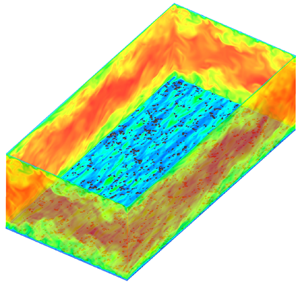
  $\delta$ is the channel half-height (figure 4
 $a$). The interfaces between the rough tiles are set equal to the average value of the adjacent roughness heights, and periodicity is enforced in streamwise and spanwise directions. The test section height is 25 mm in the turbulent channel facility, as mentioned by Flack et al. (Reference Flack, Schultz and Barros2020). The length, width and height of the rough surface are all therefore scaled by the channel half-height of 12.5 mm. The rough surface is visualized in figure 4
 $(b)$.

Figure 4.  $(a)$ The tiled surfaces with their physical boundaries (solid black) and turbulent channel domain (dashed red).
  $(b)$ Illustration of the rough surface height.
At the beginning of a simulation, the experimental roughness heights are interpolated to the computational mesh in the  $x\text {--}z$ plane. These interpolated roughness heights are then resolved in the
  $y$ direction to obtain the final rough surface used in the simulation. All cells that share a face with a fluid cell are tagged as boundary cells. Boundary cells can be either an edge cell (if the boundary cell borders exactly one fluid cell) or a corner cell (if the boundary cell shares a corner with two or more fluid cells). The momentum equations are solved inside the fluid domain while the pressure is solved in both fluid and solid domains. No-slip boundary conditions are applied at the faces of boundary cells. As a result, face-normal velocities are set to zero at the boundaries independent of the cell centre value. This ensures that the pressure values inside the solid domain do not affect the pressure values in the fluid domain.
The characteristic parameters of the rough surface in Case R400 are compared with those of the original tiles in table 2, and good agreement is observed. The p.d.f. of the processed rough surface in the simulations is compared with the original tiles in figure 5 $(a)$. Good agreement is observed in the p.d.f., which is well approximated by a Gaussian distribution. The extent of discrepancies at small scales due to the surface processing is illustrated by comparing energy spectra of the original rough tile with that of the processed surface for Case R400 in figure 5
 $(b)$. The radial wavenumber is
  $k=\sqrt {k_x^2+k_z^2}$, where
  $k_x$ and
  $k_z$ are the streamwise and spanwise wavenumbers normalized by the length
  $L_x$ and width
  $L_z$ of the channel domain, respectively. The processed surface has a cut-off radial wavenumber at
  $k=80$ (dotted line) compared with the original tile. The two-dimensional power spectrum of the original surface is shown in figure 5
 $(c)$. The ‘cross-pattern’ is caused by the aliasing effects at the non-periodic boundaries of the original rough tiles. Figure 6 shows a direct comparison of a portion of the surface profile between the original and processed surface. Note that the small scales are smoothed out but the profile remains a reasonable approximation.
Table 2. Surface statistics of the computational rough surface in Case R400, compared with the experimental tiles. The roughness height is in millimetres.


Figure 5.  $(a)$ The p.d.f. of the roughness height for the processed rough surfaces of Case R400 (dashed red) and Case R600 (dash-dotted blue), compared with the original surface tiles (solid black) and a Gaussian (long-dashed grey) with the same
  $k_{rms}$.
  $(b)$ Energy spectrum of the processed surface compared with the original tile.
  $(c)$ Two-dimensional spectrum of the original tile. The circle indicates the cut-off radial wavenumber after processing the surface.

Figure 6. Comparison of a portion of the computational surface with the experimental scan. The solid black line shows the experimental surface, and the dashed red line shows the computational rough surface for Case R400. The symbols show the face velocities on the boundaries.
3.2. Problem description
Simulations are performed at  $Re_{\tau }=u_{\tau } \delta /\nu =400$ and
  $600$, where
  $u_{\tau }$ is the friction velocity,
  $\delta =(L_y-y_0)/2$ is the channel half-height and
  $y_0$ is the reference bottom plane, which is taken to be the arithmetic mean height of the roughness. The rough surface described in § 3.1 is used as the bottom wall. No-slip boundary conditions are applied on both the top and bottom walls and periodicity is enforced in the streamwise (
 $x$) and spanwise (
 $z$) directions; non-uniform grids are used in the wall-normal (
 $y$) direction where the grid is clustered near the rough-wall region. Domain sizes and relevant grid details are summarized in table 3. The random rough simulation at
  $Re_{\tau }=400$ is denoted by Case R400 and that at
  $Re_{\tau }=600$ is denoted by Case R600. The value of
  $k_s^+$ is equal to 6.4 for Case R400 and 9.6 for Case R600.
Table 3. Simulation parameters for the rough-channel simulations.

The computational time step  $\Delta t$ is
  $5 \times 10^{-4} \delta / u_{\tau }$. In order to achieve statistical convergence, mean quantities and statistics were averaged over a period
  $T=50 \delta / u_{\tau }$. Since the roughness leads to spatial heterogeneity of the time-averaged variables, the DA decomposition (Raupach & Shaw Reference Raupach and Shaw1982) is applied:
 \begin{equation} \theta(x,y,z,t) = \langle \bar{\theta} \rangle(y) + \tilde{\theta}(x,y,z) + \theta'(x,y,z,t). \end{equation}
Here,  $\theta$ represents an instantaneous flow variable and
  $\bar {\theta }$ denotes its time average. The instantaneous turbulent fluctuation is
  $\theta '=\theta -\bar {\theta }$. The brackets denote the spatial-averaging operator:
 \begin{equation} \langle \bar{\theta} \rangle(y) = 1/A_f\int \int_{A_f} \bar{\theta}(x,y,z)\,\mathrm{d}x\, \mathrm{d}z, \end{equation}
where  $A_f$ is the fluid-occupied area. This means that when calculating
  $\langle \bar {\theta } \rangle (y)$ in the rough regions, only the fluid cells are taken into account. The summation of
  $\bar {\theta }$ over the fluid cells at each
  $y$ location is then divided by the number of fluid cells at the corresponding
  $y$ location. The form-induced dispersive component,
  $\tilde {\theta }$, is defined as
  $\tilde {\theta }=\bar {\theta }-\langle \bar {\theta } \rangle$, which represents the spatial variation of the time-averaged flow quantities.
According to the decomposition in (3.1), the Reynolds stress tensor is defined as
 \begin{equation} \overline{u_i'u_j'} = \overline{(u_i-\overline{u_i})(u_j-\overline{u_j})} \end{equation}
and the dispersive stress tensor is defined as
 \begin{equation} \widetilde{u_i}\widetilde{u_j} = (\overline{u_i}-\langle \overline{u_i} \rangle)(\overline{u_j}-\langle \overline{u_j} \rangle). \end{equation}
 For compactness, the streamwise mean velocity is denoted by  $U$ where the overline (denoting temporal averaging) and angle brackets (denoting spatial averaging) are dropped:
 \begin{equation} U(y) = \left\langle \bar{u} \right\rangle = 1/A_f \int \int_{A_f} \bar{u}(x,y,z)\, \mathrm{d}x\,\mathrm{d}z. \end{equation}
The bulk velocity is defined as
 \begin{equation} U_b = (1/L_y) \int_{y_o}^{L_y} U(y)\,\mathrm{d}y. \end{equation}
The spatial averages of the Reynolds stress tensor are denoted by  $\langle u_i'u_j' \rangle$ after dropping the overbar. The average wall shear stress is
  $\tau _w=\rho \delta K_1$. Since the top wall is smooth and the bottom wall is rough, the shear stress over the smooth wall,
  ${\tau }_{w}^{t}$, is calculated by averaging
  $\mu (\partial \bar u/\partial y)|_{y=L_y}$ over the wall. The rough-wall shear stress
  ${\tau }_{w}^{b}$ is then computed from the force balance between the drag of the walls and the constant pressure gradient. The bottom wall friction velocity is then calculated as
  $u_{\tau }^{b}=({\tau }_{w}^{b}/\rho )^{1/2}$.
3.3. Grid convergence
A grid convergence study is performed for the two  $Re_{\tau }$, using finer grid simulations denoted by cases R400f and R600f. Details of the simulation are listed in table 3. A smaller domain is used for Case R400f to reduce the computational cost, while the normal domain is used for Case R600f. Past studies of smooth turbulent channel (Lozano-Durán & Jiménez Reference Lozano-Durán and Jiménez2014) and turbulent channel with urban-like cubical obstacles (Coceal et al. Reference Coceal, Thomas, Castro and Belcher2006) suggest that a domain size of
  $L_x \times L_z=4\delta \times 2.4\delta$ is sufficient for obtaining mean and turbulent statistics without any significant confinement effects.
The wall-normal grid resolution for DNS in rough-wall channel flows depends on the roughness topography and the strength of roughness effects on the flow. Busse et al. (Reference Busse, Lützner and Sandham2015) recommended  $\Delta y^+ <1$ within the roughness layer and a maximum resolution of
  $\Delta y^+ \approx 5$ at the centreline of the channel for transitionally rough cases. For the present simulations, the grid resolution is comparable to that used by Busse et al. (Reference Busse, Lützner and Sandham2015) in the wall-normal direction. The streamwise and spanwise resolutions also adhere to the criteria suggested by Busse et al. (Reference Busse, Lützner and Sandham2015). The smallest roughness wavelength is resolved by
  $14$ grid points.
For Case R400f, two original rough tiles are interpolated onto grids of size  $667\times 200$. The interpolated tiles are then randomly rotated and tiled in the spanwise direction to achieve a domain size of
  $4\delta \times 2.4\delta$. The length scales of the rough surface are normalized by the channel half-height of 12.5 mm. For Case R600f, since the wall-normal resolution of Case R600 is sufficiently fine, the grid is refined in the streamwise and spanwise directions. The mean velocity and Reynolds stress profiles from the finer grids are compared with those from cases R400 and R600 in figure 7. Good agreement is observed between both profiles.

Figure 7. The grid-refined cases R400f and R600f compared with R400 and R600:  $(a{,}c)$ mean velocity profile normalized with average friction velocity
  $u_{\tau }$ and
  $(b{,}d)$ Reynolds stresses normalized with
  $u_{\tau }^2$.
Figure 8 shows the time-averaged velocity profiles in the roughness layer for a few randomly chosen points. Note that the velocity profiles drop to zero at the surface and that the profiles for coarse and fine grids are in acceptable agreement, indicating that the flow is adequately resolved.

Figure 8. Time-averaged streamwise velocity profiles within the roughness layer at a few random locations on the rough surface.
4. Results
4.1. Skin-friction coefficient
The mean skin-friction coefficient is  $C_f={\tau }_{w}^{b}/({\rho } U_b^{2}/2)$, where
  $U_b$ is the bulk velocity. Figure 9 compares the computed values of
  $C_f$ at the two
  $Re_{\tau }$ to the experimental results of Flack et al. (Reference Flack, Schultz and Barros2020). Note that the rough surface is nearly hydraulically smooth at the lower Reynolds number. The skin-friction coefficient decreases as
  $Re$ increases and the flow becomes transitionally rough. Both the viscous drag and form drag contribute to the overall skin friction in this flow regime. As
  $Re$ further increases, the rough surface exhibits fully rough behaviour where the skin friction becomes independent of
  $Re$. The
  $C_f$ values of Case R400 and Case R600 are shown in table 4. The errors of the simulation relative to the experiment at the two
  $Re_{\tau }$ are
  $0.8\,\%$ and
  $0.3\,\%$, respectively, showing acceptable agreement.

Figure 9. Skin-friction coefficient of cases R400 and R600, compared with experimental results (Flack et al. Reference Flack, Schultz and Barros2020). The rough surfaces correspond to the surface with  $k_{rms}\approx 88\ \mathrm {\mu }\textrm {m}$ and
  $Sk=-0.07$ in Flack et al. (Reference Flack, Schultz and Barros2020).
Table 4. Skin-friction coefficient from experiments.

4.2. Double-averaged velocity
The DA velocity profiles for cases R400 and R600 are discussed below. Figure 10 $(a)$ shows the streamwise mean velocity profile in outer coordinates. Parameter
  $U$ is normalized by the average friction velocity
  $u_{\tau }$ and
  $y$ is shifted by subtracting the reference plane
  $y_0$, and then normalized by
  $\delta$. The smooth cases at
  $Re_{\tau }=395$ and
  $Re_{\tau }=590$ from Moser et al. (Reference Moser, Kim and Mansour1999) are also presented for comparison. A velocity deficit can be observed for the rough cases and the velocity decrease is more significant in the lower half-channel. Compared with the smooth case, the peak of the mean velocity profile at
  $Re_{\tau }=400$ decreases by
  $1.6\,\%$ and shifts away from the rough wall by
  $5\,\%$. For the higher
  $Re_{\tau }$, a more significant velocity deficit is observed. The peak mean velocity is reduced by
  $4.4\,\%$ and shifted by
  $8.4\,\%$ compared with the smooth case at the same
  $Re_{\tau }$.

Figure 10. Mean velocity profile normalized by  $(a)$ average friction velocity
  $u_{\tau }$ and
  $(b)$ rough-wall friction velocity
  $u_{\tau }^b$, compared with DNS of smooth channel flow of Moser et al. (Reference Moser, Kim and Mansour1999). The vertical dotted lines in
  $(b)$ denote the top of the roughness layer,
  $k_c^+$.
Figure 10 $(b)$ provides a closer view of the viscous wall region for the rough wall. The mean velocity and the wall-normal distance of the smooth cases are normalized by the average friction velocity
  $u_{\tau }$ and
  $\nu /u_{\tau }$, respectively. The smooth-wall curves at different
  $Re_{\tau }$ collapse in inner coordinates. Scaling with the bottom-wall friction velocity
  $u_{\tau }^{b}$ provides a more accurate representation of slip and drag effects (e.g. Alamé & Mahesh Reference Alamé and Mahesh2019). Hence, for the rough cases, the mean velocity profile of the lower half-channel is normalized by
  $u_{\tau }^{b}$. Case R400 shows a slip velocity at the wall and the profile is lowered by
  $6.7\,\%$ relative to the smooth case. The slip velocity is increased further for Case R600 and the profile is shifted downwards by
  $13.2\,\%$. The two profiles intersect at
  $y^{+}=5.7$. This indicates that a larger slip velocity exists at the wall and an overall increase of drag is exhibited in the viscous wall region as
  $Re_{\tau }$ increases.
The mean velocity profile is shown in figure 11 $(a)$ using the same scaling as figure 10
 $(b)$, but in semi-log coordinates. Due to the slip effect of the roughness, the velocity profile shows a gradual increase away from the wall. This trend appears to end at
  $y^{+}=5$ which is the transition from the viscous sublayer to the buffer layer. In the buffer layer, the velocity for Case R600 increases more slowly and displays a more significant velocity deficit than Case R400. A similar trend was observed by Busse et al. (Reference Busse, Thakkar and Sandham2017). In the logarithmic-law region, the smooth-wall profiles follow the logarithmic law:
 \begin{equation} U_{s}^{+}=\frac{1}{\kappa} \ln{y^{+}}+ B, \end{equation}
where  $\kappa$ is the von Kármán constant and
  $B$ is the intercept for a smooth wall. The rough-wall profiles conform to the logarithmic law but display an offset from the smooth-wall profiles, where the roughness effect on mean velocity can be evaluated from this difference. Nikuradse (Reference Nikuradse1933) found that the logarithmic velocity distribution for the mean velocity profile still held for rough walls, with the same value of
  $\kappa$ as
 \begin{equation} U_{r}^{+}=\frac{1}{\kappa} \ln({y/k_{s}})+ 8.5. \end{equation}
The roughness function is obtained by taking the difference of mean velocities in wall units between smooth and rough walls within the logarithmic layer:
 \begin{equation} B-\Delta U^{+}+\frac{1}{\kappa} \ln{k_{s}^{+}}=8.5. \end{equation}
Flack & Schultz (Reference Flack and Schultz2010) show good collapse in the fully rough regime for different roughness types when using  $k_{s}$ as the roughness scale. However, in the transitional regime, the roughness function depends on the roughness type, and the onset of the fully rough regime is unknown for most surfaces. Difference
  $\Delta U^{+}$ from the simulations is plotted in figure 11
 $(b)$ as a function of the corresponding roughness Reynolds number
  $k_{s}^{+}$ obtained from experiment. The results show that cases R400 and R600 are in the transitionally rough regime, and match the experimental results of Flack et al. (Reference Flack, Schultz and Barros2020).

Figure 11.  $(a)$ Mean velocity profile in the bottom half of the channel in inner coordinates. The legend is the same as figure 10.
  $(b)$ Roughness function compared with the experimental results of Flack et al. (Reference Flack, Schultz and Barros2020) and the fully rough asymptote.
4.3. Reynolds stresses
The Reynolds stresses scaled by  $u_{\tau }^{2}$ are shown in outer coordinates in figure 12. The location of the peak of
  $\langle u'u' \rangle ^+$ is dependent on
  $Re$, as shown in figure 12
 $(a)$, hence both smooth and rough cases at
  $Re_{\tau }=600$ are closer to the wall than at
  $Re_{\tau }=400$. The peak of
  $\langle u'u' \rangle ^+$ in the lower half-channel for Case R400 is decreased by
  $2.8\,\%$ compared with the smooth wall of Moser et al. (Reference Moser, Kim and Mansour1999). This behaviour is consistent with Busse et al. (Reference Busse, Lützner and Sandham2015). The minimum value is shifted to the top wall by
  $7.9\,\%$ due to the asymmetry induced by the roughness. For
  $Re_{\tau }=600$, the peak value of
  $\langle u'u' \rangle ^+$ is further decreased by
  $9.1\,\%$ and the minimum value is shifted to the top wall by
  $9.2\,\%$; i.e. the roughness has a more significant effect on the streamwise velocity fluctuations as
  $Re_{\tau }$ increases.

Figure 12. Reynolds stress profiles normalized by  $u_{\tau }$:
  $(a)$ streamwise,
  $(b)$ wall-normal and
  $(c)$ spanwise components and
  $(d)$ Reynolds shear stress. The legend is the same as figure 10.
The wall-normal Reynolds stress is shown in figure 12 $(b)$. Compared with the smooth channel,
  $\langle v'v' \rangle ^+$ in the lower half-channel is increased, while that in the upper half-channel is decreased. The peak value of
  $\langle v'v' \rangle ^+$ in the lower half-channel is increased by
  $5.3\,\%$ at
  $Re_{\tau }=400$ and
  $8.9\,\%$ at
  $Re_{\tau }=600$. The spanwise velocity fluctuations also increase in the lower half-channel (figure 12
 $c$), and they decrease in the upper half-channel compared with the smooth channel. The Reynolds shear stress increases in magnitude at the rough wall, (figure 12
 $d$), consistent with the increase in wall-normal velocity fluctuations. The profile of
  $\langle u'v' \rangle ^+$ shifts downwards by
  $4.9\,\%$ at
  $Re_{\tau }=400$ and by
  $8.4\,\%$ at
  $Re_{\tau }=600$.
The Reynolds stresses are normalized by the local friction velocity at each wall and plotted separately in figure 13. This scaling yields better collapse in the logarithmic regions of the smooth and rough walls. In the near-wall region of the rough wall, the peak value of the streamwise component of the rough-wall side decreases. The spanwise component shows a higher peak value while the wall-normal component and Reynolds shear stress show relatively weaker variation in their peak values. These trends become more pronounced with increasing  $Re_{\tau }$.

Figure 13. Near-wall Reynolds stresses scaled by local friction velocity  $u_{\tau }^l=u_{\tau }^b$ for the bottom wall and
  $u_{\tau }^t$ for the top wall.
  $(a)$ Case R400 and
  $(b)$ Case R600. The vertical dashed line denotes the top of the roughness layer
  $k_c^+$.
Busse et al. (Reference Busse, Lützner and Sandham2015) studied a series of surfaces with different levels of filtering (a low-pass filter was used to remove the high-wavenumber contributions to the surface data). For their smallest roughness height ( $k_{rms}^+=4.6$) and largest skewness (
 $Sk=1.15$, where
  $Sk>0$ means the surface is peak-dominant), they found an increase in the peak of
  $\langle v'v'\rangle ^+$, and a slight increase in both
  $\langle v'v'\rangle ^+$ and
  $\langle u'v'\rangle ^+$ in the roughness layer. Compared with their surfaces, the present rough surfaces have smaller roughness heights in wall units for cases R400 and R600, and zero skewness. That is, our surfaces have fewer, and smaller, asperities to increase
  $\langle v'v'\rangle ^+$ and
  $\langle u'v'\rangle ^+$.
4.4. Dispersive flux and correlations
The dispersive stresses obtained from DA are examined in the near-wall region of the rough wall in figure 14. Compared with the Reynolds stresses, the dispersive stresses are mostly confined to the roughness layer, consistent with the observations of Yuan & Jouybari (Reference Yuan and Jouybari2018) and Jelly & Busse (Reference Jelly and Busse2019). For Case R400,  $\langle \tilde {u} \tilde {u} \rangle ^+$ is maximum at
  $(y-y_0)/\delta =0.015$ and drops to zero by
  $(y-y_0)/\delta =0.05$, underlining the importance of spatial inhomogeneity in the roughness layer. The profiles of
  $\langle \tilde {v} \tilde {v} \rangle ^+$ and
  $\langle \tilde {w} \tilde {w} \rangle ^+$ peak at
  $(y-y_0)/\delta =0.011$ and
  $0.016$, respectively. The dispersive shear stress
  $\langle \tilde {u} \tilde {v} \rangle ^+$ shows the same peak location as
  $\langle \tilde {v} \tilde {v} \rangle ^+$ and is comparatively small. The level of dispersive stresses is enhanced for higher
  $Re_{\tau }$, especially in the roughness layer, and the peak values occur closer to the wall.

Figure 14. Dispersive stress profiles scaled by  $u_{\tau }^b$ over the bottom half of the channel. The vertical dotted line denotes the top of the roughness layer
  $k_c$. The legend of
  $(b)$ is same as
  $(a)$.
Dispersive stresses arise from regions where the local temporal average is different from the average computed over time and the entire rough wall. The form-induced velocity and pressure are examined at  $(y-y_0)/\delta =0.0075$ and
  $z/\delta =1.57$ in figure 15 to illustrate how the roughness topography contributes to the local inhomogeneity in the roughness layer. Figure 15
 $(a)$ shows that large positive
  $\tilde {u}$ (red region) occurs in the large trough regions between roughness asperities, while large negative
  $\tilde {u}$ (blue region) occurs in the wake regions behind the roughness elements. Both these high- and low-momentum regions contribute to the streamwise dispersive stress. In the areas where the roughness protrusions are relatively peaky and dense, corresponding to the
  $x$–
$x$– $y$ plane probed in figure 15
 $(b)$, regions with negative
  $\tilde {u}$ are observed near the roughness protrusions.

Figure 15. Form-induced quantities for Case R400 at  $(y-y_0)/\delta =0.0075$ (
 $y^+=3$): (
 $a$)
$a$)  $\tilde {u}^+$, (
 $c$)
$c$)  $\tilde {v}^+$, (
 $e$)
$e$)  $\tilde {w}^+$, (
 $g$)
$g$)  $\tilde {p}^+$. A slice at
  $z/\delta =1.57$: (
 $b$)
$b$)  $\tilde {u}^+$, (
 $d$)
$d$)  $\tilde {v}^+$, (
 $\,f$)
  $\tilde {w}^+$, (
 $h$)
$h$)  $\tilde {p}^+$. The velocities are normalized by
  $u_{\tau }^b$ and pressure is normalized by
  $(u_{\tau }^b)^2$. The rectangular regions labelled by
  $A$ and
  $B$ are two representative roughness geometries discussed in the text.
Figures 15 $(c)$ and 15
 $(d)$ show that impulsive upward velocities, shown by the high-magnitude positive
  $\tilde {v}$ (red regions), occur mostly in front of the roughness protrusions. Downward velocities, shown by the negative
  $\tilde {v}$ (blue regions), occur in the wake of the protrusions. The strength of these upward and downward motions is positively correlated with the roughness height.
Figures 15 $(e)$ and 15
 $(\,f)$ show pairs of large positive
  $\tilde {w}$ (red region) and negative
  $\tilde {w}$ (blue region) in front of the roughness crests. This suggests that the impulsive upward velocity produces a pair of streamwise vortices in front of the roughness elements. Similar behaviour was observed by Muppidi & Mahesh (Reference Muppidi and Mahesh2012) in their investigation of an idealized rough-wall supersonic boundary layer. Also,
  $\tilde {v}$ displays larger wall-normal length scales than
  $\tilde {w}$, which explains why the peak location of
  $\langle \tilde {v} \tilde {v} \rangle ^+$ is higher than that of
  $\langle \tilde {w} \tilde {w} \rangle ^+$ in figure 14
 $(b)$.
The pressure perturbations at the same locations are shown in figures 15 $(g)$ and 15
 $(h)$. High
  $\tilde {p}$ (red region) is found to occur in front of the roughness asperities where the flow stagnates, while low
  $\tilde {p}$ (blue region) occurs at the crests and behind the roughness elements. The form drag is therefore mainly produced by the peaks of the rough surface.
The form-induced quantities for Case R600 were also examined but are not shown here in the interests of brevity. The main features remain the same, while their magnitudes increase at the higher  $Re_{\tau }$.
Figure 16 takes a closer look at how roughness protrusions contribute to mean wall-normal fluxes. Two representative regions labelled  $A$ and
  $B$ in figure 15
 $(b)$ are considered. Region
  $A$ represents a dense and peaky region where the flow is dominated by negative
  $\tilde {u}$, while
  $B$ is a relatively flat and smooth region. Both figures 16
 $(a)$ and 16
 $(b)$ show that negative
  $\tilde {u}$ is induced at the back of the protrusions, and the largest crest yields the strongest negative
  $\tilde {u}$. The upward
  $\tilde {v}$ induced in front of the crests accompanies the negative
  $\tilde {u}$, resulting in ‘ejection’ motions, borrowing terminology from the boundary layer literature (Bailey & Stoll Reference Bailey and Stoll2013). Similar strong ‘ejection’ motions are present in front of the crests while ‘sweeping’ motions occur within the troughs. Both ‘ejection’ and ‘sweeping’ motions are responsible for the negative dispersive shear stress shown in figure 14
 $(b)$. A clockwise ‘roll-up’ motion is shown at the roughness crests in figure 16
 $(b)$; such motions occur when the surface topography is less rough and the flow is not dominated by negative
  $\tilde {u}$. Thus roughness geometry influences wall-normal momentum transfer by influencing the ‘ejection’ and ‘roll-up’ motions.

Figure 16. Vectors of ( $\tilde {u}$,
 $\tilde {v}$) with background contours of
  $\tilde {p}^+$ for representative roughness sections, corresponding to the regions labelled (
 $a$)
$a$)  $A$ and (
 $b$)
$b$)  $B$ in figure 15
 $(b)$.
Figure 17 shows the joint p.d.f. of ( $\tilde {u}$,
  $\tilde {p}$) and (
 $\tilde {v}$,
  $\tilde {p}$) near the roughness mean height at
  $y^+=3$ for Case R400. The results for Case R600 are not shown since the main conclusions remain the same. Stronger correlations between
  $\tilde {u}$ and
  $\tilde {p}$ are observed in the third quadrant
  $Q3$ compared with the smooth channel (Lenaers et al. Reference Lenaers, Li, Brethouwer, Schlatter and Örlü2012), which corresponds to the ‘roll-up’ motions induced by the roughness crests. The regions with these motions account for the negative
  $\tilde {u}$ and correlate with the negative
  $\tilde {p}$, as shown in figure 16
 $(b)$. Lenaers et al. (Reference Lenaers, Li, Brethouwer, Schlatter and Örlü2012) found a correlation between negative
  $v$ and positive
  $p'$ near smooth walls, indicating splatting events. In the rough case, however, the correlation in the second quadrant
  $Q2$ is weak since positive
  $p'$ is more due to stagnation on the roughness elements. Meanwhile, the correlation in
  $Q1$ and
  $Q3$ is stronger since the upward
  $\tilde {v}$ is always induced in front of the crests where positive
  $\tilde {p}$ occurs, while the downward
  $\tilde {v}$ appears in the wake regions where negative
  $\tilde {p}$ occurs.

Figure 17. Joint p.d.f. of  $(a)$ (
 $\tilde {u}^+$,
  $\tilde {p}^+$) and
  $(b)$ (
 $\tilde {v}^+$,
  $\tilde {p}^+$) for Case R400 at the wall-normal location
  $(y-y_0)/\delta =0.0075$ (
 $y^+=3$). Contour levels are defined by the common logarithm of joint p.d.f. and the interval between successive contour levels is 0.5.
4.5. Mean momentum balance
The mean momentum balance reveals the different contributions to momentum conservation in the roughness layer. The streamwise DA momentum equation for a fully developed channel flow (Raupach & Shaw Reference Raupach and Shaw1982; Yuan & Jouybari Reference Yuan and Jouybari2018) is
 \begin{equation} \underbrace{\frac{\partial \langle \tilde{u} \tilde{v} \rangle}{\partial y}}_{\text{A}} = -\underbrace{\frac{\partial \langle \bar{p} \rangle}{\partial x}}_{\text{B}} + \underbrace{\nu \frac{\partial^2 \langle \bar{u} \rangle}{\partial y^2}}_{\text{C}} -\underbrace{ \left \langle \frac{\partial \tilde{p} }{\partial x} \right \rangle}_{\text{D}} + \underbrace{\nu \left \langle \frac{\partial^2 \tilde{u} }{\partial x_j^2}\right \rangle}_{\text{E}} - \underbrace{\frac{\partial \langle \overline{u'v'} \rangle}{\partial y}}_{\text{F}} + \langle K \rangle, \end{equation}
where the subscript  $j$ denotes streamwise, wall-normal and spanwise components for position vectors and
  $K$ is the constant pressure gradient (divided by density). In this equation, term A is the dispersive shear stress gradient, term B represents the mean pressure gradient which is zero in our simulations, term C shows the viscous force (viscous stress gradient), terms D and E account for the pressure drag and viscous drag caused by the roughness, respectively, and term F is the net effect of turbulent inertia (Reynolds stress gradient).
Figure 18 shows the budget of terms in the mean momentum equation for the bottom half-channel. Since terms A, D and E are zero for Case SW, the balance is among the constant pressure gradient, the viscous and Reynolds stress gradients. For Case R400, the Reynolds stress gradient is slightly increased at the wall and the peak but follows a similar variation as Case SW in general. As  $y^+$ increases, the viscous stress gradient increases and reaches a maximum value at
  $y^+=3$, then decreases to negative values and collapses with Case SW above the roughness layer. The pressure and viscous drag are induced by the roughness and only exist in the roughness layer. Compared with other terms, the contribution of the dispersive term is quite small. Overall, the roughness transfers mean momentum downward through the viscous and Reynolds stress gradients to balance the pressure and viscous drag. The observation for Case R600 is the same except that the magnitude of each term is larger than for Case R400.

Figure 18. Budget of the streamwise DA momentum equation for Case SW (symbols) and Case R400 (lines). The vertical dotted line denotes the top of the roughness layer  $k_c^+$. The summation of all terms is denoted by the short-dashed line.
4.6. Pressure fluctuations
4.6.1. Mean-square pressure fluctuations
Figure 19 $(a)$ shows the mean-square pressure fluctuations
  $\langle \overline {p'p'} \rangle ^+$ in outer coordinates for cases R400 and R600 over the bottom half of the channel. Also shown are Case SW and other smooth channel flows from Panton et al. (Reference Panton, Lee and Moser2017). Note that away from the wall, both smooth- and rough-wall curves collapse on to the logarithmic correlation described by Panton et al. (Reference Panton, Lee and Moser2017):
 \begin{equation} \langle \overline{p'p'} \rangle^+_{cp}(y/\delta) = -2.5625\ln(y/\delta) + 0.2703. \end{equation}
As  $Re_{\tau }$ increases,
  $\langle \overline {p'p'} \rangle ^+$ increases near the wall, peaks closer to the wall and collapses onto the logarithmic correlation closer to the wall. Roughness increases the peak levels of
  $\langle \overline {p'p'} \rangle ^+$ near the wall.

Figure 19.  $(a)$ Profiles of mean-square pressure fluctuations
  $\langle \overline {p'p'} \rangle$ normalized by
  $u_{\tau }^b$ and
  $(b)$ inner correlation
  $\langle \phi \rangle (y^+)$. Symbols denote: Case SW (solid), Case R400 (circle), Case R600 (delta), Panton et al. (Reference Panton, Lee and Moser2017),
  $Re_{\tau }=182$ (dashed),
  $Re_{\tau }=544$ (dash-dotted),
  $Re_{\tau }=1001$ (dash-dot-dot). The vertical dashed lines denote the roughness layers.
Panton et al. (Reference Panton, Lee and Moser2017) derived an inner correlation to account for the  $Re_{\tau }$ dependence for smooth channel flows:
 \begin{equation} \langle \phi \rangle(y^+) = \langle \overline{p'p'} \rangle^+(y^+,Re_{\tau}) - 2.5625\ln(Re_{\tau}) - 0.2703. \end{equation}
Figure 19 $(b)$ shows
  $\langle \phi \rangle (y^+)$ computed for both smooth and rough cases. The smooth curves show acceptable collapse both near to and away from the wall for all
  $Re_{\tau }$. The rough curves, however, collapse only beyond
  $y^+=50$. The increased level of pressure fluctuations below
  $y^+=50$ indicates that the roughness increases the pressure fluctuations in the inner layer and the enhancement is much stronger for higher
  $Re_{\tau }$.
The vertical lines in figure 19 $(b)$ illustrate the top of the roughness layer. Note that
  $\langle \overline {p'p'} \rangle ^+$ peaks outside the roughness layer. Comparing Case R400 with Case SW, the level of pressure fluctuations within the roughness layer increases by
  $20.2\,\%$, and the peak value by
  $7.8\,\%$. For Case R600, the enhancement of pressure fluctuations in the roughness layer is even higher.
The spatial variation of  $\overline {p'p'}$ is examined at a representative location
  $(y-y_0)/\delta =0.0075$ and
  $z/\delta =1.57$ in figure 20. At both Reynolds numbers, high pressure fluctuations are observed in front of the roughness asperities, while the regions behind the roughness elements have lower levels. The unsteady stagnation and wake regions induced by the roughness elements result in higher pressure fluctuations. Smooth-wall flows do not display this behaviour, and hence have lower levels of pressure fluctuations for the same
  $Re_{\tau }$.

Figure 20. Mean-square pressure fluctuations  $\overline {p'p'}$ normalized by
  $U_b$ for Case R400 at (
 $a$)
$a$)  $(y-y_0)/\delta =0.0075$ (corresponding to
  $y^+=3$), (
 $b$)
$b$)  $z/\delta =1.57$, and Case R600 at (
 $c$)
$c$)  $(y-y_0)/\delta =0.0075$ (corresponding to
  $y^+=4.5$) and (
 $d$)
$d$)  $z/\delta =1.57$.
4.6.2. Poisson equation source terms
The source terms in the pressure Poisson equation provide further insight into how roughness influences pressure fluctuations. The Poisson equation for the fluctuating pressure is given by
 \begin{equation} \frac{\partial^2 p'}{\partial x_i \partial x_i} = - 2 \frac{\partial {\langle \overline{u_i} \rangle}}{\partial {x_j}}\frac{\partial u_j'}{\partial x_i} - \frac{\partial^2}{\partial x_i \partial x_j}\left(u_i'u_j' - \overline{u_i'u_j'}\right). \end{equation}
The first term on the right-hand side is called the mean-shear or rapid source term (MS) and the second term is known as the turbulence-turbulence or slow source term (TT). The dominant component of the MS term is
 \begin{equation} MS_{12} = - 2 \frac{\partial {\langle \bar{u} \rangle}}{\partial {y}}\frac{\partial v'}{\partial x}. \end{equation}
Since this term involves the streamwise mean velocity gradient, it is large near the wall (Johansson, Her & Haritonidis Reference Johansson, Her and Haritonidis1987). For the TT term, it has been shown that the component
 \begin{equation} TT_{23}=\frac{\partial {v'}}{\partial {z}}\frac{\partial w'}{\partial y} - \frac{\partial ^2 \overline{v'w'}}{\partial y \partial z} \end{equation}
is the dominant term, located in the buffer region whose peak location is correlated with the average position of quasi-streamwise vortices (Chang III et al. Reference Chang III, Piomelli and Blake1999). The dominant terms  $MS_{12}$ and
  $TT_{23}$ for the random rough channel flows are discussed below.
Figure 21 shows how roughness impacts  ${\partial {\langle \bar {u} \rangle }}/{\partial {y}}, {\partial v'}/{\partial x}$ and
  $MS_{12}$ individually. The profiles are normalized by the local friction velocity at the two walls. Roughness is seen to affect both the mean and fluctuating velocity gradients. Figure 21
 $(a)$ shows that for the smooth half of the channel, the mean velocity gradient is largest at the wall and gradually decreases with increasing
  $y$. On the other hand, at the rough wall,
  ${\partial {\langle \bar {u} \rangle }}/{\partial {y}}$ peaks at
  $y^+=6$ which lies within the roughness layer, and collapses onto the smooth-wall profile for larger
  $y$. Figure 21
 $(b)$ shows
  $\partial {v'} /\partial x$. Note that the r.m.s. of
  $\partial {v'} /\partial x$ significantly increases within the roughness layer, and collapses with the smooth-wall profile above the roughness. Both terms combine to increase
  $MS_{12}$ as shown in figure 21
 $(c)$. The peak values are within the roughness layer at
  $y^+=6$, consistent with the peak locations observed in figure 21
 $(a)$. Both Reynolds numbers show the same behaviour except that Case R600 has higher magnitudes.

Figure 21.  $(a)$ Streamwise mean velocity gradient,
  $(b)$
$(b)$  $\partial {v'} /\partial x$,
  $(c)$
$(c)$  $MS_{12}$ and
  $(d)$
$(d)$  $TT_{23}$. Here
  $u_{\tau }^l$ and
  $\delta$ are used for normalization. The vertical dash-dotted line denotes the mean roughness height
  $y=y_0$, and the vertical dashed lines denote the top of the roughness layer
  $k_c^+$.
Figures 22 $(a)$ and 22
 $(b)$ show the local variation of r.m.s.
  $MS_{12}$ in the near-wall region for Case R400. The intense high-magnitude spots (red regions) are produced in front of the roughness protrusions and on the crests. The time-averaged spanwise vorticity in figures 22
 $(c)$ and 22
 $(d)$ shows the local mean shear layers that form at the same locations. These shear layers combine to yield the mean velocity gradient at a wall-normal location. The higher levels of
  $\partial {v'} /\partial x$ within the roughness layer are due to the upward velocity in front of the protrusions and the ‘roll-up’ motions on the crests observed in § 4.4.

Figure 22. Spatial variation of r.m.s.  $MS_{12}$ for Case R400 at
  $(a)$
$(a)$  $y^+=3$ and
  $(b)$
$(b)$  $z^+=628$. Time-averaged spanwise vorticity
  $\overline {\omega _z}$ normalized by
  $u_{\tau }/\delta$ at
  $(c)$
$(c)$  $y^+=3$ and
  $(d)$
$(d)$  $z^+=628$. The dashed line in
  $(a)$ denotes the
  $x^+$–
 $y^+$ plane observed in
  $(b)$ and
  $(d)$, while the dashed line in
  $(b)$ denotes the edge of the roughness layer.
The high-magnitude regions of r.m.s.  $MS_{12}$ and
  $\overline {\omega _z}^+$ are consistent with the regions of high pressure fluctuations in figure 20. The more intense pressure fluctuations in front of and above the roughness elements can be attributed to the attached shear layers formed upstream of the obstacles. The low level of r.m.s.
  $MS_{12}$ in the wake regions is because the flow is more quiescent behind the roughness elements.
The r.m.s. of  $TT_{23}$ is examined in figure 21
 $(d)$. Note that for both cases R400 and R600, the level of
  $TT_{23}$ increases in the roughness layer, the peak location remains at
  $y^+=18$ and the profile above the roughness layer collapses with that of the smooth wall. The spatial distribution of r.m.s.
  $TT_{23}$ at
  $y^+=3$ and
  $x^+=688$ for Case R400 is shown in figures 23
 $(a)$ and 23
 $(b)$, respectively. The high-magnitude regions (red) are observed as the streaky structures in the troughs as well as a large band at
  $y^+=18$. To specifically investigate how the r.m.s. of
  $TT_{23}$ is increased in the roughness layer, two typical high-magnitude streaks are identified in figure 23
 $(a)$ and the time-averaged streamwise vorticity in the corresponding
  $z$–
$z$– $y$ planes are examined in figures 23
 $(c)$ and 23
 $(d)$. Two main features are identified. For location A, the level of
  $TT_{23}$ is increased in the immediate vicinity upstream of the roughness protrusion. Meanwhile, a pair of streamwise vortices is observed at the same location which is induced by the upward velocity in front of the protrusions. A pair of secondary vortices is observed below the induced streamwise vortices, closely attaching to the bottom wall. For location B, the high-magnitude streak is located in the valley in the same region where the streamwise vortices occur. These observations show that
  $TT_{23}$ is correlated with the quasi-streamwise vortices. Since quasi-streamwise vortices are present in the troughs (Jouybari, Brereton & Yuan Reference Jouybari, Brereton and Yuan2019) and induced in front of the protrusions, the r.m.s. of
  $TT_{23}$ is accordingly increased.

Figure 23. Spatial variation of r.m.s.  $TT_{23}$ for Case R400 at
  $(a)$
$(a)$  $y^+=3$ and
  $(b)$
$(b)$  $x^+=xu_{\tau }/\nu =688$. Time-averaged streamwise vorticity
  $\overline {\omega _x}$ normalized by
  $u_{\tau }/\delta$ corresponding to
  $(c)$ the square region A at
  $x^+=160$ and
  $(d)$ the square region B at
  $x^+=688$. The dashed lines in
  $(a)$ denote the
  $z^+$–
 $y^+$ planes observed in
  $(b\text {--}d)$, while the dashed line in
  $(b)$ denotes the edge of the roughness layer. Note that for the
  $z^+$–
 $y^+$ plane, the mean flow direction points out of the page.
The flow characteristics related to the contributions of  $MS_{12}$ and
  $TT_{23}$ to the pressure fluctuations are summarized in figure 24. The shear layer along with the ‘roll-up’ motion indicated by the dashed ellipse is generated at the upstream stagnation point of the protrusion in figure 24
 $(a)$, and is a primary source of the larger pressure fluctuations. Figure 24
 $(b)$ illustrates the streamwise vortices that occur in front of the protrusion and also in the troughs, generating secondary vortical structures below the main vortices.

Figure 24. Illustration of the typical flow features contributing to  $(a)$
$(a)$  $MS_{12}$ and
  $(b)$
$(b)$  $TT_{23}$. The dashed ellipse in
  $(a)$ denotes the shear layer formed on the protuberance. The red arrows in
  $(b)$ represent a pair of streamwise vortices and secondary vortices beneath them.
4.7. Wall shear stress fluctuations
The effects of roughness on wall shear stress fluctuations are examined in this section. The wall shear stress components  $\tau _{yx}$ and
  $\tau _{yz}$ are calculated at the rough surface. Data are collected for a time period
  $T=32\delta /u_{\tau }$ with sampling time interval
  $t=2.5\times 10^{-3}\delta /u_{\tau }$. The wall shear stress fluctuations are denoted by
  $\tau _{yx}'$ and
  $\tau _{yz}'$, the time-averaged values are expressed as
  $\overline {\tau _{yx}}$ and
  $\overline {\tau _{yz}}$ and the r.m.s. values are
  $\tau _{yx,rms}$ and
  $\tau _{yz,rms}$.
4.7.1. Local variation of wall shear stress
Shear stress  $\overline {\tau _{yx}}$ and the roughness height for a portion of the surface are shown in figure 25. The results of Case R400f are compared with those of Case R400 and found to be in acceptable agreement.

Figure 25. Roughness height and time-averaged streamwise wall shear stress for a portion of the rough surface. The red circles denote locations A–E where wall shear stress is probed.
Figure 25 shows that the variation of  $\overline {\tau _{yx}}$ in the rough case is highly correlated with the roughness height. Parameter
  $\overline {\tau _{yx}}$ has large positive values at the roughness protrusions, and is nearly zero or has small negative values in the valleys.
Five different locations (see table 5) on the roughness profile in figure 25 are probed to show the dependence of wall shear on the surface topography. Point A is located at a trough, where  $\overline {\tau _{yx}}$ is negative, due to the reverse flow that occurs in the trough. Points B, C and D have a similar
  $y^+$. However, B is at a trough where
  $\overline {\tau _{yx}}$ is close to zero. Point C is located at the ascent of the protrusion, which shows a higher
  $\overline {\tau _{yx}}$ and
  $\tau _{yx,rms}$. In contrast to points B and C, point D is located at a crest, leading to even larger mean and r.m.s. of wall shear stress. The wall shear stress at the crest for an even higher
  $y^+$ is examined at point E. The mean and r.m.s. values are much higher than those of other probed locations.
Table 5. Locations and time-averaged and r.m.s. values of  $\tau _{yx}$ for the probed points in figure 25.

4.7.2. Probability distribution function of wall shear stress
The effect of roughness on the p.d.f. of wall shear stress is examined. The p.d.f.s of the streamwise shear stress component  $\tau _{yx}$, spanwise shear stress component
  $\tau _{yz}$ and the shear stress yaw angle
  $\phi _{\tau } = \tan ^{-1}(\tau _{yz}(t)/\tau _{yx}(t))$ are shown in figure 26, and tabulated in table 6. Case SW is the baseline, whose statistics of wall shear stress fluctuations show good agreement with the results for a smooth-wall turbulent boundary layer (Diaz-Daniel et al. Reference Diaz-Daniel, Laizet and Vassilicos2017). Motivated by the influence of topography in § 4.7.1, the shear stress is probed separately in two regions: the ‘peak region’ (above the mean height location) and the ‘valley region’ (below the mean height location). A schematic of the decomposition is shown in figure 27.

Figure 26. The p.d.f.s of  $(a)$ streamwise wall shear stress,
  $(b)$ spanwise wall shear stress and
  $(c)$ angle between shear stress vector and streamwise direction. Cases SW (solid black), R400 peak (dashed red), R400 valley (dash-dotted red), R600 peak (long-dashed blue) and R600 valley (dash-dot-dot blue).

Figure 27. Illustration of how wall shear stress is divided into peak regions (above the mean height location) and valley regions (below the mean height location).
Table 6. Statistics of the wall shear stress components  $\tau _{yx}$,
  $\tau _{yz}$ and yaw angle
  $\phi _{\tau }$: mean
  $\mu (\cdot )$, standard deviation
  $\sigma (\cdot )$, skewness
  $Sk(\cdot )$ and kurtosis
  $Ku(\cdot )$.

The r.m.s. of the streamwise shear stress for Case SW (table 6) is in good agreement with the correlation  $\tau _{yx,rms}^{+}=\tau _{yx,rms}/\tau _{w}=0.298+0.018\ln Re_{\tau }$, proposed by Örlü & Schlatter (Reference Örlü and Schlatter2011). Comparison of the rough walls with Case SW at the same
  $Re_{\tau }$ reveals the following features. A significant increase in the probability of events with positive
  $\tau _{yx}$ is observed for the peak region in figure 26
 $(a)$ since
  $\tau _{yx}$ is associated with the streamwise velocity which generally increases as
  $y$ increases. The probability of events with negative
  $\tau _{yx}$ is higher in the valleys, corresponding to figure 28 that shows how reverse flows occur mainly in the valleys. The p.d.f. for rough surfaces has longer tails (larger kurtosis), since intermittent events in the flow can interact randomly with peaks or valleys in the rough surface, resulting in more extreme events.

Figure 28. Contours of time-averaged streamwise velocity and vectors of ( $\bar {u}$,
 $\bar {v}$) in the vicinity of the rough surface for Case R400.
The p.d.f. of spanwise wall shear stress fluctuations  $\tau _{yz}$, shown in figure 26
 $(b)$, has zero mean and zero skewness for both smooth and rough cases. The normalization by the r.m.s. values collapses the peak of the p.d.f.; however, the tails are longer for the rough walls. This behaviour is more pronounced at the higher
  $Re_{\tau }$.
The probability distribution of  $\phi _{\tau }$ in figure 26
 $(c)$ examines the correlation between
  $\tau _{yx}$ and
  $\tau _{yz}$. Jeon et al. (Reference Jeon, Choi, Yoo and Moin1999) found that the probability for events with
  $|\phi _{\tau }|>45^{\circ }$ is very small in smooth channel flows; i.e. the flow is dominated by events where large positive
  $\tau _{yx}$ is associated with small
  $\tau _{yz}$. The standard deviation of
  $\phi _{\tau }$ is much higher for the rough wall, compared with Case SW. The probability of events with
  $|\phi _{\tau }| >45^{\circ }$ is enhanced by the roughness, suggesting that the events with comparable magnitudes of
  $\tau _{yx}$ and
  $\tau _{yz}$ occur more frequently. This behaviour can be explained by the three-dimensionalization of the vortical motions in the roughness layer. The roughness elements break up the directional bias of the near-wall streaks and generate more isotropic vorticity fields (Mehdi, Klewicki & White Reference Mehdi, Klewicki and White2010; Jouybari et al. Reference Jouybari, Brereton and Yuan2019). In the valley region, events with
  $90^{\circ } < |\phi _{\tau }| <180^{\circ }$ (corresponding to negative
  $\tau _{yx}$) are more probable, consistent with reverse flow in the valleys. The p.d.f. of
  $|\phi _{\tau }|$ tends to be more evenly distributed for Case R600, implying that the reverse flow is enhanced as
  $Re_{\tau }$ increases.
5. Summary
Direct numerical simulation of turbulent channel flow with an irregular rough wall is performed at  $Re_{\tau }=400$ and
  $600$. The rough wall is generated from experimental line scans (Flack et al. Reference Flack, Schultz and Barros2020). Statistics, spectra and p.d.f.s of the computational surface are ensured to be in good agreement with the experiment. No-slip Dirichlet boundary conditions are imposed on the rough surface in the simulations, and grid convergence studies are conducted to establish that the flow is adequately resolved. The roughness height has Gaussian p.d.f., and
  $k_s^+$ is equal to 6.4 and 9.6 for
  $Re_{\tau }=400$ and
  $600$, respectively. The roughness height is smaller than that of most past rough-wall studies and the flow is in the transitionally rough regime.
The computed skin-friction coefficients and roughness functions agree with those measured by Flack et al. (Reference Flack, Schultz and Barros2020). When scaled with the global friction velocity, the streamwise fluctuations decrease from their smooth-wall values, while wall-normal and spanwise fluctuations, and the Reynolds shear stress increase in magnitude at the rough wall. Scaling using the local friction velocity reveals that the peak value of streamwise velocity fluctuations decreases while the spanwise velocity fluctuations increase. The wall-normal velocity fluctuations and Reynolds shear stress show relatively weaker variation. The near-wall motions and momentum transfer due to the roughness are studied using DA statistics. ‘Ejection’ and ‘roll-up’ motions on the roughness crests are found to alter the wall-normal momentum transfer. Form drag is produced mainly by the roughness protrusions, and the negative and positive  $\tilde {p}$ contributing to the form drag are correlated with negative
  $\tilde {u}$ and positive
  $\tilde {v}$, respectively. The mean momentum is transferred downward by the viscous force and turbulence inertia, to balance the total drag induced by the roughness.
Roughness effects on pressure fluctuations are investigated. Pressure fluctuation amplitudes increase in the roughness layer, and collapse with the smooth-wall levels away from the wall. Their spatial variation suggests that the higher pressure fluctuations are due to the unsteady stagnation and wake regions induced by the roughness elements. As  $Re_{\tau }$ increases, roughness effects on pressure fluctuations are enhanced. The dominant source terms in the pressure Poisson equation,
  $MS_{12}$ and
  $TT_{23}$, are examined. Roughness causes the mean shear to peak within the roughness layer, while also increasing
  $\partial v^\prime /\partial x$, both of which combine to increase
  $MS_{12}$ within the roughness layer. The local variation of
  $MS_{12}$ suggests the mean shear layers on the roughness protrusions as the primary source of increased pressure fluctuations. Term
  $TT_{23}$ is enhanced in the troughs and upstream of the protrusions, and is associated with the streamwise vortices at these locations.
The effects of roughness on wall shear stress are examined. The time-average and r.m.s. of  $\tau _{yx}$ is positively correlated with the roughness height, and highly dependent on the local roughness topography. The p.d.f.s of wall shear stress fluctuations are examined for the influence of topography. The probability of events with positive
  $\tau _{yx}$ is found to be higher in the peak regions since
  $\tau _{yx}$ is associated with the streamwise velocity which generally increases as
  $y$ increases. The probability of events with negative
  $\tau _{yx}$ is higher in the valley regions, since reverse flow occurs mainly in the valleys. Surface roughness increases the probability of extreme events since intermittent events in the flow can interact randomly with peaks or valleys in the rough surface. Events with comparable magnitudes of
  $\tau _{yx}$ and
  $\tau _{yz}$ occur more frequently since the roughness elements break up the directional bias of near-wall streaks. These effects are more pronounced at the higher
  $Re_{\tau }$.
Acknowledgements
This work was supported by the United States Office of Naval Research (ONR) Grant N00014-17-1-2308 managed by Drs J. Gorski, T. Fu and P. Chang. Computing resources were provided by the Minnesota Supercomputing Institute (MSI). We are grateful to Professor K. Flack at the United States Naval Academy for providing us with the scanned surface data used in the present work. The authors would like to thank Mr S. Anantharamu, Dr P. Kumar and Dr Y. Li for their helpful discussions and suggestions.
Declaration of interests
The authors report no conflict of interest.


