1 Introduction
The present work aims at investigating the large-scale dynamics of compressible homogeneous isotropic turbulence in the presence of strong dense gas effects. Dense gases (DG) are usually defined as single-phase fluids, characterized by complex molecules, working in pressure and temperature conditions of the same order of magnitude as their thermodynamic critical point (see, e.g. Cinnella & Congedo Reference Cinnella and Congedo2007 and references cited therein). Dense gas fluid dynamics is governed by a thermodynamic parameter known as the fundamental derivative of gas dynamics (Thompson Reference Thompson1971), defined as
 $$\begin{eqnarray}{\it\Gamma}:=\frac{v^{3}}{2c^{2}}\left.\frac{\partial ^{2}p}{\partial v^{2}}\right|_{s}=1+\frac{{\it\rho}}{c}\left.\frac{\partial c}{\partial {\it\rho}}\right|_{s},\end{eqnarray}$$
where
 ${\it\rho}$
is the density,
${\it\rho}$
is the density,
 $v$
the specific volume,
$v$
the specific volume,
 $p$
the pressure,
$p$
the pressure,
 $s$
the entropy and
$s$
the entropy and
 $c=\sqrt{\partial p/\partial {\it\rho}|_{s}}$
the sound speed. The first equality in the preceding definition shows that
$c=\sqrt{\partial p/\partial {\it\rho}|_{s}}$
the sound speed. The first equality in the preceding definition shows that
 ${\it\Gamma}$
is related to the curvature of isentropic lines in the
${\it\Gamma}$
is related to the curvature of isentropic lines in the
 $p{-}v$
plane; according to the second definition,
$p{-}v$
plane; according to the second definition,
 ${\it\Gamma}$
is a measure of the rate of change of the sound speed in isentropic transformations. From (1.1),
${\it\Gamma}$
is a measure of the rate of change of the sound speed in isentropic transformations. From (1.1),
 ${\it\Gamma}<1$
implies
${\it\Gamma}<1$
implies
 $\partial c/\partial {\it\rho}|_{s}<0$
, meaning that the sound speed grows in isentropic expansions and drops in isentropic compressions, unlike the case of perfect gases, where:
$\partial c/\partial {\it\rho}|_{s}<0$
, meaning that the sound speed grows in isentropic expansions and drops in isentropic compressions, unlike the case of perfect gases, where:
 $$\begin{eqnarray}{\it\Gamma}=\frac{{\it\gamma}+1}{2},\end{eqnarray}$$
 ${\it\gamma}=c_{p}/c_{v}$
being the ratio of the isobaric specific heat
${\it\gamma}=c_{p}/c_{v}$
being the ratio of the isobaric specific heat
 $c_{p}$
to the isochoric specific heat
$c_{p}$
to the isochoric specific heat
 $c_{v}$
. For thermodynamic stability,
$c_{v}$
. For thermodynamic stability,
 ${\it\gamma}$
is always greater than unity, hence
${\it\gamma}$
is always greater than unity, hence
 ${\it\Gamma}>1$
for perfect gases. On the contrary, heavy gases characterized by high
${\it\Gamma}>1$
for perfect gases. On the contrary, heavy gases characterized by high
 $c_{v}/R$
ratios (
$c_{v}/R$
ratios (
 $R$
being the gas constant), exhibit extended ranges of density and pressures in which
$R$
being the gas constant), exhibit extended ranges of density and pressures in which
 ${\it\Gamma}$
is less than unity, or even negative, the perfect gas behaviour being recovered in the low-density limit.
${\it\Gamma}$
is less than unity, or even negative, the perfect gas behaviour being recovered in the low-density limit.
Dense gas flows exhibit interesting physical behaviours that are not yet fully understood. The most interesting phenomena are expected for a family of heavy polyatomic compounds, named Bethe–Zel’dovich–Thompson (BZT) fluids (Bethe Reference Bethe1942; Zel’Dovich & Raizer Reference Zel’Dovich and Raizer1966; Thompson Reference Thompson1971), which exhibit a region of negative
 ${\it\Gamma}$
values (called the ‘inversion zone’, see Cramer & Kluwick Reference Cramer and Kluwick1984) in the vapour phase close to the liquid/vapour coexistence curve. This is theoretically predicted to result in non-classical compressibility effects in the transonic and supersonic flow regimes, such as rarefaction shock waves, mixed shock/fan waves and shock splitting (see e.g. Cramer & Kluwick Reference Cramer and Kluwick1984; Cramer Reference Cramer1989b
, Reference Cramer1991 and Rusak & Wang Reference Rusak and Wang1997). Furthermore, the entropy change across a weak shock, given by Bethe (Reference Bethe1942):
${\it\Gamma}$
values (called the ‘inversion zone’, see Cramer & Kluwick Reference Cramer and Kluwick1984) in the vapour phase close to the liquid/vapour coexistence curve. This is theoretically predicted to result in non-classical compressibility effects in the transonic and supersonic flow regimes, such as rarefaction shock waves, mixed shock/fan waves and shock splitting (see e.g. Cramer & Kluwick Reference Cramer and Kluwick1984; Cramer Reference Cramer1989b
, Reference Cramer1991 and Rusak & Wang Reference Rusak and Wang1997). Furthermore, the entropy change across a weak shock, given by Bethe (Reference Bethe1942):
 $$\begin{eqnarray}{\rm\Delta}s=-\frac{c^{2}{\it\Gamma}}{v^{3}}\frac{({\rm\Delta}v)^{3}}{6T}+O(({\rm\Delta}v)^{4})\end{eqnarray}$$
with
 $T$
the absolute temperature, is much weaker than usual for dense gases with
$T$
the absolute temperature, is much weaker than usual for dense gases with
 ${\it\Gamma}\ll 1$
, leading to reduced shock losses. Note that, if
${\it\Gamma}\ll 1$
, leading to reduced shock losses. Note that, if
 ${\it\Gamma}<0$
, then
${\it\Gamma}<0$
, then
 ${\rm\Delta}s>0$
only if
${\rm\Delta}s>0$
only if
 ${\rm\Delta}v>0$
, meaning that expansion shocks are admissible according to the second principle of thermodynamics.
${\rm\Delta}v>0$
, meaning that expansion shocks are admissible according to the second principle of thermodynamics.
For dense gases, the perfect gas (PFG) model is no longer valid, and more complex equations of state (EoS) are used to account for their peculiar thermodynamic behaviour. One of the simplest models for dense gases is the Van der Waals (VDW) EoS (Van der Waals Reference Van der Waals1873), which takes into account the co-volume occupied by the molecules and the two-body collision interactions. The VDW EoS allows us to predict the inflexion of the critical isotherm at the critical point (
 $p/p_{c}=1$
,
$p/p_{c}=1$
,
 $v/v_{c}=1$
; subscript
$v/v_{c}=1$
; subscript
 $(\cdot )_{c}$
indicates the critical conditions) and the change of curvature of the isotherms in the Clapeyron plane
$(\cdot )_{c}$
indicates the critical conditions) and the change of curvature of the isotherms in the Clapeyron plane
 $p-v$
for
$p-v$
for
 ${\it\Gamma}=0$
. As a consequence, VDW is also the simplest possible EoS allowing us to account for the BZT effects (Bethe Reference Bethe1942).
${\it\Gamma}=0$
. As a consequence, VDW is also the simplest possible EoS allowing us to account for the BZT effects (Bethe Reference Bethe1942).
Turbulent flows of dense gases are of interest for a wide range of engineering applications, such as energy conversion cycles (Monaco, Cramer & Watson Reference Monaco, Cramer and Watson1997; Brown & Argrow Reference Brown and Argrow2000; Horen et al. Reference Horen, Talonpoika, Larjola and Siikonen2002), high Reynolds number wind tunnels (Anderson Reference Anderson1991), chemical transport and processing (Kirillov Reference Kirillov2004) and refrigeration (Zamfirescu & Dincer Reference Zamfirescu and Dincer2009).
Considerable progress has been made in the past 30 years about the study of inviscid dense gas flows. Inviscid flows of dense gases have been extensively studied analytically, with focus on the generation of non-classical compressibility effects such as expansion shocks, sonic and double-sonic shocks and shock splitting (Thompson & Lambrakis Reference Thompson and Lambrakis1973; Cramer & Kluwick Reference Cramer and Kluwick1984; Cramer & Sen Reference Cramer and Sen1987; Cramer Reference Cramer1989a
,Reference Cramer
b
; Menikoff & Plohr Reference Menikoff and Plohr1989; Cramer Reference Cramer1991; Cramer & Tarkenton Reference Cramer and Tarkenton1992; Cramer & Fry Reference Cramer and Fry1993; Rusak & Wang Reference Rusak and Wang1997; Wang & Rusak Reference Wang and Rusak1999; Rusak & Wang Reference Rusak and Wang2000), both for one-dimensional unsteady and two-dimensional steady configurations. For the case of viscous dense gases, analytical studies were carried out to investigate the dissipative structure of shock waves and the impact of dense gas effects on laminar boundary layers and laminar shock/boundary layer interactions (Cramer & Crickenberger Reference Cramer and Crickenberger1991; Cramer & Park Reference Cramer and Park1999; Kluwick Reference Kluwick2004; Kluwick & Wrabel Reference Kluwick and Wrabel2004; Kluwick & Meyer Reference Kluwick and Meyer2010, Reference Kluwick and Meyer2011). These studies pointed out that it is possible to greatly reduce, or even suppress, the separation induced by shock/boundary layer interactions for some optimal choice of the operating thermodynamic state. Moreover, dense gases are generally characterized by heat capacities much larger than those of gases of less molecular complexity, leading to small characteristic Eckert numbers (
 $Ec=U_{ref}/(c_{p}T_{ref})$
, with
$Ec=U_{ref}/(c_{p}T_{ref})$
, with
 $U_{ref}$
and
$U_{ref}$
and
 $T_{ref}$
a reference velocity and temperature, respectively). Hence, the coupling between the dynamic and thermal boundary layers is much weaker than in flows of standard gases like air.
$T_{ref}$
a reference velocity and temperature, respectively). Hence, the coupling between the dynamic and thermal boundary layers is much weaker than in flows of standard gases like air.
Theoretical findings have been confirmed by numerical simulations. Computations of inviscid dense gas flows have been presented, among others, by Argrow (Reference Argrow1996), Brown & Argrow (Reference Brown and Argrow1998), Cinnella & Congedo (Reference Cinnella and Congedo2005). Cinnella & Congedo (Reference Cinnella and Congedo2007) performed the first numerical simulation of turbulent dense gas flows. Specifically, they investigated compressible turbulent boundary layers and transonic turbulent flows around airfoils by using the Reynolds-averaged Navier–Stokes (RANS) equations closed by standard turbulence models. The simulations were carried out under a set of working assumptions, namely: (i) the flow conditions being sufficiently far from the thermodynamic critical point, dramatic variations of the fluid specific heats and compressibility coefficients, as well as density fluctuations were neglected; (ii) the compressible RANS equations supplemented by an eddy viscosity turbulence model were supposed to provide an adequate description of the mean flow for the configurations under study; (iii) the turbulent heat transfer was modelled though a ‘turbulent Fourier law’, by introducing a turbulent Prandtl number, assumed to be roughly constant and of
 $O(1)$
throughout the flow, as commonly done in PFG flows.
$O(1)$
throughout the flow, as commonly done in PFG flows.
More recently, several other authors have carried out RANS simulations of turbulent dense gas flows, in particular for turbomachinery applications (e.g. Harinck et al. Reference Harinck, Turunen-Saaresti, Colonna, Rebay and van Buijtenen2010; Wheeler & Ong Reference Wheeler and Ong2013, Reference Wheeler and Ong2014; Sciacovelli & Cinnella Reference Sciacovelli and Cinnella2014). However, the accuracy of RANS models for these flows has not been properly assessed up to now, due to the lack of reference data either experimental or numerical. In particular, reliable experimental results are extremely difficult to obtain – most attempts of constructing dense gas shock tube and nozzle experiments are at the preliminary design stage as yet – and all of the past and present attempts aim at getting experimental proofs of the existence of non-classical shock waves, rather than providing detailed turbulence data. For single-phase gases close to saturation conditions, the most impressive non-classical phenomenon, i.e. the formation of a rarefaction shock wave, has been observed experimentally by Borisov et al. (Reference Borisov, Borisov, Kutateladze and Nakaryakov1983) and Kutateladze, Nakaryakov & Borisov (Reference Kutateladze, Nakaryakov and Borisov1987); however, the interpretation of such results has been challenged by several authors (Cramer & Sen Reference Cramer and Sen1986; Fergason et al. Reference Fergason, Ho, Argrow and Emanuel2001). More recently, dense gas shock tubes and test rigs have been devised by Fergason et al. (Reference Fergason, Ho, Argrow and Emanuel2001), Colonna et al. (Reference Colonna, Guardone, Nannan and Zamfirescu2008), Spinelli et al. (Reference Spinelli, Dossena, Gaetani, Osnaghi and Colombo2010), but no experimental results have been published to the present date.
High-fidelity numerical datasets such as those provided by direct numerical simulations (DNS) represent an effective tool for gaining insight into the physics of turbulent dense gas flows. In the literature, DNS have been carried out for low Mach number turbulent flows of light supercritical fluids such as carbon dioxide and nitrogen, with a focus on heat-transfer properties, the so-called piston effect and dissipation effects in mixing layers (Zappoli et al.
Reference Zappoli, Bailly, Garrabos, Le Neindre, Guenoun and Beysens1990; Okong’o & Bellan Reference Okong’o and Bellan2002; Bae, Yoo & Choi Reference Bae, Yoo and Choi2005; Okong’o & Bellan Reference Okong’o and Bellan2010; Tanahashi et al.
Reference Tanahashi, Tominaga, Shimura, Hashimoto and Miyauchi2011). Selle & Schmitt (Reference Selle and Schmitt2010) have studied the influence of supercritical initial conditions on the decay of homogeneous turbulence for nitrogen, assumed to obey a cubic EoS, even though their analysis is limited to the study of the kinetic energy decay evolution at low turbulent Mach number (
 $M_{t}=0.1$
). At these conditions, compressibility effects are negligible and the authors conclude that real gas thermodynamic effects have a negligible influence on the turbulence dynamics. Battista, Picano & Casciola (Reference Battista, Picano and Casciola2014) extended the low Mach number Navier–Stokes equations for reactive perfect gas flows to a generic real gas equation of state. They analysed the turbulent mixing of slightly supercritical fluids at low Mach number by means of the VDW EoS, and found differences in the ligament structures. Much less is known about turbulent dense gas flows in the transonic and supersonic regime. The impact of dense gas effects on compressible homogeneous isotropic turbulence (CHIT) and, more generally, highly compressible dense gas turbulent flows, represents an open research field.
$M_{t}=0.1$
). At these conditions, compressibility effects are negligible and the authors conclude that real gas thermodynamic effects have a negligible influence on the turbulence dynamics. Battista, Picano & Casciola (Reference Battista, Picano and Casciola2014) extended the low Mach number Navier–Stokes equations for reactive perfect gas flows to a generic real gas equation of state. They analysed the turbulent mixing of slightly supercritical fluids at low Mach number by means of the VDW EoS, and found differences in the ligament structures. Much less is known about turbulent dense gas flows in the transonic and supersonic regime. The impact of dense gas effects on compressible homogeneous isotropic turbulence (CHIT) and, more generally, highly compressible dense gas turbulent flows, represents an open research field.
In this work, we investigate for the first time the impact of dense gas effects on the structure of compressible turbulence, with focus on high Reynolds number flows that are of interest for typical dense gas industrial applications. As a natural starting point, we select a configuration that has been well documented for perfect gases, namely, the decay of high turbulent Mach number CHIT in a periodic box, which may exhibit eddy shocklets. For this kind of flow, the peculiar behaviour of the speed of sound when
 ${\it\Gamma}$
is close to or less than zero is expected to modify the turbulence structure significantly. Specifically, for turbulent flows of BZT fluids, non-classical eddy shocklets may appear, leading to significant changes in the probability distribution functions of several flow properties. In decaying CHIT, the turbulent Mach number decreases with time. As a consequence, dense gas effects are expected to have an impact most of all on the initial stages of the decay, which are dominated by large to medium scales of turbulence.
${\it\Gamma}$
is close to or less than zero is expected to modify the turbulence structure significantly. Specifically, for turbulent flows of BZT fluids, non-classical eddy shocklets may appear, leading to significant changes in the probability distribution functions of several flow properties. In decaying CHIT, the turbulent Mach number decreases with time. As a consequence, dense gas effects are expected to have an impact most of all on the initial stages of the decay, which are dominated by large to medium scales of turbulence.
Much of the numerical work on incompressible or perfect gas CHIT is restricted to low/moderate Taylor-based Reynolds numbers (generally less than 500, see Wang et al. (Reference Wang, Shi, Wang, Xiao, He and Chen2012), Donzis & Jagannathan (Reference Donzis and Jagannathan2016)), restricting severely the range of scales in the inertial range undergoing a cascade mechanism unimpeded by dissipative processes (Porter, Woodward & Pouquet Reference Porter, Woodward and Pouquet1998). Addressing high Reynolds numbers is more difficult as the turbulent Mach number of the simulation increases. Dissipative processes are, of course, fundamental at the smallest scales, where the turbulent kinetic energy is converted into heat. For high Reynolds number incompressible isotropic decaying turbulence, Lesieur (Reference Lesieur2008) identified two distinct stages: in the first stage, viscous effects are negligible, worm-like structures due to sheet roll-up development, and vortex stretching causes a large increase of enstrophy; in the second stage of the decay, the energy transferred to the smallest scales by means of the energy cascade mechanism start to be dissipated by viscosity. The transition from the first to the second stage corresponds to a peak in the time history of the total enstrophy, since no smaller structures can be created in the second phase and the existing ones are destroyed due to viscous effects. Lesieur then concludes that the initial stages of the decay are well represented by an inviscid model.
Euler-based turbulent simulations have been largely employed in the literature to investigate the behaviour of high Reynolds number supersonic turbulent flows, such as wakes of objects moving at supersonic speed or those encountered in the interstellar medium. High-resolution numerical simulations of both forced and decaying inviscid supersonic turbulence have been performed by Porter, Pouquet & Woodward (Reference Porter, Pouquet and Woodward1992a ,Reference Porter, Pouquet and Woodward b , Reference Porter, Pouquet and Woodward1994), Porter et al. (Reference Porter, Woodward and Pouquet1998, Reference Porter, Pouquet, Sytine and Woodward1999), Porter, Pouquet & Woodward (Reference Porter, Pouquet and Woodward2002), Sytine et al. (Reference Sytine, Porter, Woodward, Hodson and Winkler2000), who provided information about the spectra, intermittency, energy transfers and scaling exponents for structure functions of velocity, density and entropy. For decaying turbulence, the impact of dilatational modes on the different temporal phases has been addressed by Kritsuk et al. (Reference Kritsuk, Norman, Padoan and Wagner2007), who performed large-scale three-dimensional (3-D) simulations of supersonic inviscid turbulence. They measured the velocity scaling exponents and the slope of the velocity power spectrum, finding substantial differences with respect to incompressible turbulence, and proposed an extension of Kolmogorov’s theory taking into account compressibility effects. Benzi et al. (Reference Benzi, Biferale, Fisher, Kadanoff, Lamb and Toschi2008) performed high-resolution numerical simulations of homogeneous isotropic inviscid weakly compressible turbulence. They showed that the scaling properties of the velocity field in the inertial range were in excellent agreement with those observed in DNS of the Navier–Stokes equations. One important result of the studies cited above is that the dynamics of the inertial range is independent not only of viscosity but also of the detailed dynamics of the dissipative mechanism. As a consequence, the latter does not affect the statistical properties in the inertial range. Similar considerations have led several investigators to model the small-scale dissipative processes using hyperviscosity algorithms, e.g. Cook & Cabot (Reference Cook and Cabot2005), Lamorgese, Caughey & Pope (Reference Lamorgese, Caughey and Pope2005).
Based on the above-mentioned results, in the present paper we adopt the Euler equations, written for gases governed by a general equation of state. The governing equations are discretized by using a ninth-order accurate scheme, which introduces a numerical dissipation based on tenth-order derivatives in smooth flow regions. This dissipates wavelengths close to the grid cutoff, while leaving larger scales almost unaffected.
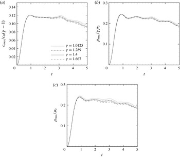
The paper is organised as follows. The governing equations and the numerical method are described in § 2. Details of the numerical set-up (initial and boundary conditions) adopted for the CHIT simulations, as well as a validation against literature results for a PFG, are provided in § 3. In addition, in § 3 we also discuss the validity of the inviscid assumption by comparison with viscous results at various Reynolds numbers. Dense gases are characterized by values of the specific heat ratio closer to unity than diatomic gases like air or triatomic gases like carbon dioxide (see, e.g. Harinck, Guardone & Colonna Reference Harinck, Guardone and Colonna2009). As a consequence, deviations with respect to classical PFG simulations for a diatomic gas can be due both to the different specific ratio and to the EoS. In order to distinguish the contributions of these two effects, in § 4.1 we present a preliminary study of the sensitivity of PFG solutions to the specific heat ratio of the gas. In § 4.2, dense gas compressible homogeneous isotropic turbulence at various initial turbulent Mach numbers is investigated by using the VDW model, and the results are compared with those of a PFG characterized by the same heat ratio. The main findings of the study are summarized in § 5.
2 Governing equations and numerical scheme
The flow model is based on the compressible Euler equations, whose validity for large-scale dynamics is discussed in § 3.2. The equations, written in integral form for a control volume
 $\mathscr{V}$
with boundary
$\mathscr{V}$
with boundary
 $\partial \mathscr{V}$
, are:
$\partial \mathscr{V}$
, are:
 $$\begin{eqnarray}\frac{\text{d}}{\text{d}t}\int _{\mathscr{V}}\boldsymbol{w}\,\text{d}\mathscr{V}+\oint _{\partial \mathscr{V}}\boldsymbol{f}\boldsymbol{\cdot }\boldsymbol{n}\,\text{d}S=0,\end{eqnarray}$$
with
 $\boldsymbol{w}=[{\it\rho},{\it\rho}\boldsymbol{v},{\it\rho}E]^{\text{T}}$
the conservative variable vector,
$\boldsymbol{w}=[{\it\rho},{\it\rho}\boldsymbol{v},{\it\rho}E]^{\text{T}}$
the conservative variable vector,
 $\boldsymbol{f}=[{\it\rho}\boldsymbol{v},{\it\rho}\boldsymbol{v}\boldsymbol{v}+p\bar{\bar{\unicode[STIX]{x1D644}}},{\it\rho}\boldsymbol{v}H]^{\text{T}}$
, the inviscid flux,
$\boldsymbol{f}=[{\it\rho}\boldsymbol{v},{\it\rho}\boldsymbol{v}\boldsymbol{v}+p\bar{\bar{\unicode[STIX]{x1D644}}},{\it\rho}\boldsymbol{v}H]^{\text{T}}$
, the inviscid flux,
 $\boldsymbol{v}$
the velocity vector,
$\boldsymbol{v}$
the velocity vector,
 $E=e+|\boldsymbol{v}|^{2}/2$
the specific total energy,
$E=e+|\boldsymbol{v}|^{2}/2$
the specific total energy,
 $H=E+p/{\it\rho}$
the specific total enthalpy,
$H=E+p/{\it\rho}$
the specific total enthalpy,
 $e$
the specific internal energy,
$e$
the specific internal energy,
 $\bar{\bar{\unicode[STIX]{x1D644}}}$
the unit tensor and
$\bar{\bar{\unicode[STIX]{x1D644}}}$
the unit tensor and
 $\boldsymbol{n}$
the outer normal to
$\boldsymbol{n}$
the outer normal to
 $\partial \mathscr{V}$
. The system is supplemented by thermal and caloric equations of state, respectively:
$\partial \mathscr{V}$
. The system is supplemented by thermal and caloric equations of state, respectively:
 $$\begin{eqnarray}p=p({\it\rho},T)\quad \text{and}\quad e=e({\it\rho},T).\end{eqnarray}$$
These satisfy the compatibility relation:
 $$\begin{eqnarray}e=e_{ref}+\int _{T_{r}}^{T}c_{v,\infty }(T^{\prime })\,\text{d}T^{\prime }-\int _{{\it\rho}_{r}}^{{\it\rho}}\left[T\left.\frac{\partial p}{\partial T}\right|_{{\it\rho}}-p\right]\frac{\text{d}{\it\rho}^{\prime }}{{\it\rho}^{\prime 2}},\end{eqnarray}$$
where the subscript
 $(\cdot )_{ref}$
indicates a reference state,
$(\cdot )_{ref}$
indicates a reference state,
 $c_{v,\infty }(T)$
is the specific heat at constant volume in the ideal gas limit and the superscript
$c_{v,\infty }(T)$
is the specific heat at constant volume in the ideal gas limit and the superscript
 $(\cdot )^{\prime }$
denotes auxiliary integration variables. For a thermally and calorically perfect gas, (2.2) become:
$(\cdot )^{\prime }$
denotes auxiliary integration variables. For a thermally and calorically perfect gas, (2.2) become:
 $$\begin{eqnarray}p={\it\rho}RT\quad \text{and}\quad e=c_{v}T,\end{eqnarray}$$
with
 $c_{v}=R/({\it\gamma}-1)=\text{constant}$
and
$c_{v}=R/({\it\gamma}-1)=\text{constant}$
and
 $R=\mathscr{R}/\mathscr{M}$
(being
$R=\mathscr{R}/\mathscr{M}$
(being
 $\mathscr{R}$
the universal gas constant and
$\mathscr{R}$
the universal gas constant and
 $\mathscr{M}$
the gas molecular weight).
$\mathscr{M}$
the gas molecular weight).
In this paper we use the thermal Van der Waals equation of state, which models the gas molecules as rigid spheres of given radius and subject to inter-particle attractive forces. Such EoS captures the qualitative aspects of dense gas dynamics without the complexities and computational overhead associated with more complex, and accurate, thermodynamic models (Thompson & Lambrakis Reference Thompson and Lambrakis1973). This is written:
 $$\begin{eqnarray}p=\frac{RT}{v-b}-\frac{a}{v^{2}},\end{eqnarray}$$
with:
 $$\begin{eqnarray}a=\frac{9p_{c}v_{c}^{2}}{8Z_{c}}\quad b=\frac{v_{c}}{3}.\end{eqnarray}$$
and
 $Z_{c}=p_{c}v_{c}/RT_{c}$
the critical compressibility factor. Assuming a calorically perfect (polytropic) gas and combining (2.5) and (2.3), one obtains an explicit relationship for the pressure in terms of density
$Z_{c}=p_{c}v_{c}/RT_{c}$
the critical compressibility factor. Assuming a calorically perfect (polytropic) gas and combining (2.5) and (2.3), one obtains an explicit relationship for the pressure in terms of density
 ${\it\rho}$
and internal energy
${\it\rho}$
and internal energy
 $e$
:
$e$
:
 $$\begin{eqnarray}p=\frac{({\it\gamma}-1){\it\rho}e+a{\it\rho}^{2}}{1-b{\it\rho}}-a{\it\rho}^{2}.\end{eqnarray}$$
For a polytropic gas obeying the VDW EoS, the fundamental derivative of gas dynamics becomes:
 $$\begin{eqnarray}{\it\Gamma}=\frac{1}{2}\left({\displaystyle \frac{{\it\gamma}({\it\gamma}+1)RT}{(1-b{\it\rho})^{3}}}-6a{\it\rho}\right)\left/\left({\displaystyle \frac{{\it\gamma}RT}{(1-b{\it\rho})^{2}}}-2a{\it\rho}\right)\right..\end{eqnarray}$$
A region of negative values of the fundamental derivative appears if the specific heat ratio is in the range
 $1<{\it\gamma}\leqslant 1.06$
(Thompson & Lambrakis Reference Thompson and Lambrakis1973). Figure 1 shows some iso-
$1<{\it\gamma}\leqslant 1.06$
(Thompson & Lambrakis Reference Thompson and Lambrakis1973). Figure 1 shows some iso-
 ${\it\Gamma}$
lines and the inversion zone for a VDW gas with
${\it\Gamma}$
lines and the inversion zone for a VDW gas with
 ${\it\gamma}=1.0125$
, which is roughly representative of heavy fluorocarbons.
${\it\gamma}=1.0125$
, which is roughly representative of heavy fluorocarbons.
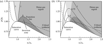
Figure 1. Clapeyron diagram for a BZT Van der Waals gas with
 ${\it\gamma}=1.0125$
. (a) The iso-
${\it\gamma}=1.0125$
. (a) The iso-
 ${\it\Gamma}$
(grey contours and solid lines) are reported as a function of
${\it\Gamma}$
(grey contours and solid lines) are reported as a function of
 $v/v_{c}$
. (b) The iso-
$v/v_{c}$
. (b) The iso-
 ${\it\Gamma}$
(grey contours) and the iso-
${\it\Gamma}$
(grey contours) and the iso-
 $c$
(solid lines) are reported as a function of
$c$
(solid lines) are reported as a function of
 $v/v_{c}$
. The dash-dotted line represents the critical isotherm
$v/v_{c}$
. The dash-dotted line represents the critical isotherm
 $T/T_{c}=1$
. In the figure the dark grey zone represents the inversion zone, corresponding to the region between the transition line and the saturation curve where
$T/T_{c}=1$
. In the figure the dark grey zone represents the inversion zone, corresponding to the region between the transition line and the saturation curve where
 ${\it\Gamma}<0$
.
${\it\Gamma}<0$
.
Table 1. Thermodynamic properties of PP11: molecular weight (
 $\mathscr{M}$
), critical temperature (
$\mathscr{M}$
), critical temperature (
 $T_{c}$
), critical density (
$T_{c}$
), critical density (
 ${\it\rho}_{c}$
), critical pressure (
${\it\rho}_{c}$
), critical pressure (
 $p_{c}$
), critical compressibility factor (
$p_{c}$
), critical compressibility factor (
 $Z_{c}$
), acentric factor (
$Z_{c}$
), acentric factor (
 ${\it\omega}$
), dipole moment of the gas phase (d.m.), boiling temperature (
${\it\omega}$
), dipole moment of the gas phase (d.m.), boiling temperature (
 $T_{b}$
) and ratio of ideal gas specific heat at constant volume over the gas constant (
$T_{b}$
) and ratio of ideal gas specific heat at constant volume over the gas constant (
 $c_{v}(T_{c})/R$
) at the critical point.
$c_{v}(T_{c})/R$
) at the critical point.

In the following simulations, we consider the perfluoro-perhydrophenanthrene, (chemical formula
 $\text{C}_{14}\text{F}_{24}$
), called hereafter PP11 (commercial name); its thermodynamic properties are provided in table 1. This fluid has been often used in the literature since it exhibits a wide inversion zone and, as a consequence, significant dense gas effects. For such a complex gas, the specific heat ratio
$\text{C}_{14}\text{F}_{24}$
), called hereafter PP11 (commercial name); its thermodynamic properties are provided in table 1. This fluid has been often used in the literature since it exhibits a wide inversion zone and, as a consequence, significant dense gas effects. For such a complex gas, the specific heat ratio
 ${\it\gamma}$
varies with the temperature. However, since the flow conditions investigated in this work are characterized by small temperature variations, we assume hereafter that
${\it\gamma}$
varies with the temperature. However, since the flow conditions investigated in this work are characterized by small temperature variations, we assume hereafter that
 ${\it\gamma}$
is constant and equal to 1.0125, which is representative of heavy fluorocarbons (Brown & Argrow Reference Brown and Argrow1998).
${\it\gamma}$
is constant and equal to 1.0125, which is representative of heavy fluorocarbons (Brown & Argrow Reference Brown and Argrow1998).
Time integration is carried out by means of a low-storage six-stage Runge–Kutta scheme (Bogey & Bailly Reference Bogey and Bailly2004). The flux derivatives in the governing equations are approximated in space by means of centred tenth-order accurate differences. In order to introduce a minimal amount of numerical dissipation while ensuring computational robustness for compressible flow simulations, the centred scheme is supplemented by a high-order artificial viscosity term, similar to the approach of Jameson, Schmidt & Turkel (Reference Jameson, Schmidt and Turkel1981) and Kim & Lee (Reference Kim and Lee2001). In our case, we use a blend of second- and tenth-order derivatives approximated by standard central differences.
For a 1-D problem and a regular Cartesian grid with constant mesh spacing
 ${\it\delta}x$
(so that
${\it\delta}x$
(so that
 $x_{j}=j\,{\it\delta}x$
), the semi-discrete tenth-order scheme in space writes:
$x_{j}=j\,{\it\delta}x$
), the semi-discrete tenth-order scheme in space writes:
 $$\begin{eqnarray}(w_{t})_{j}+\frac{({\it\delta}\mathscr{F})_{j}}{{\it\delta}x}=0,\end{eqnarray}$$
where
 ${\it\delta}$
is the classical difference operator over one cell,
${\it\delta}$
is the classical difference operator over one cell,
 ${\it\delta}(\bullet )_{j}:=(\bullet )_{j+1/2}-(\bullet )_{j-1/2}$
and
${\it\delta}(\bullet )_{j}:=(\bullet )_{j+1/2}-(\bullet )_{j-1/2}$
and
 $\mathscr{F}_{j+1/2}$
is the numerical flux at cell interface
$\mathscr{F}_{j+1/2}$
is the numerical flux at cell interface
 $j+1/2$
:
$j+1/2$
:
 $$\begin{eqnarray}\mathscr{F}_{j+1/2}=\left[\left(I-{\textstyle \frac{1}{6}}{\it\delta}^{2}+{\textstyle \frac{1}{30}}{\it\delta}^{4}-{\textstyle \frac{1}{140}}{\it\delta}^{6}+{\textstyle \frac{1}{630}}{\it\delta}^{8}\right){\it\mu}f\right]_{j+1/2},\end{eqnarray}$$
where
 $f=f(w)$
is the physical flux and
$f=f(w)$
is the physical flux and
 ${\it\mu}$
is the cell average operator,
${\it\mu}$
is the cell average operator,
 ${\it\mu}(\bullet )_{j+1/2}:=((\bullet )_{j+1}+(\bullet )_{j})/2$
. A high-order dissipation term is added to prevent high-frequency oscillations. Furthermore, the scheme is modified by introducing a nonlinear artificial viscosity term to capture flow discontinuities. The numerical flux of the scheme supplemented by the dissipation term finally becomes:
${\it\mu}(\bullet )_{j+1/2}:=((\bullet )_{j+1}+(\bullet )_{j})/2$
. A high-order dissipation term is added to prevent high-frequency oscillations. Furthermore, the scheme is modified by introducing a nonlinear artificial viscosity term to capture flow discontinuities. The numerical flux of the scheme supplemented by the dissipation term finally becomes:
 $$\begin{eqnarray}\mathscr{F}_{j+1/2}=\left[\left(I-{\textstyle \frac{1}{6}}{\it\delta}^{2}+{\textstyle \frac{1}{30}}{\it\delta}^{4}-{\textstyle \frac{1}{140}}{\it\delta}^{6}+{\textstyle \frac{1}{630}}{\it\delta}^{8}\right){\it\mu}f-\mathscr{D}\right]_{j+1/2}\end{eqnarray}$$
with the numerical dissipation term
 $\mathscr{D}$
:
$\mathscr{D}$
:
 $$\begin{eqnarray}\mathscr{D}_{j+1/2}={\it\rho}(\unicode[STIX]{x1D63C})_{j+1/2}[{\it\varepsilon}_{2}{\it\delta}w+{\it\varepsilon}_{10}{\it\delta}^{9}w]_{j+1/2}\end{eqnarray}$$
with
 ${\it\rho}(\unicode[STIX]{x1D63C})$
the spectral radius of the flux Jacobian matrix
${\it\rho}(\unicode[STIX]{x1D63C})$
the spectral radius of the flux Jacobian matrix
 $\unicode[STIX]{x1D63C}=\partial f/\partial w$
, and
$\unicode[STIX]{x1D63C}=\partial f/\partial w$
, and
 $$\begin{eqnarray}{{\it\varepsilon}_{2}}_{j+1/2}={\it\kappa}_{2}\max ({\it\nu}_{j}{\it\Phi}_{j},{\it\nu}_{j+1}{\it\Phi}_{j+1}),\quad {{\it\varepsilon}_{10}}_{j+1/2}=\max (0,k_{10}-{{\it\varepsilon}_{2}}_{j+1/2}),\end{eqnarray}$$
with
 $k_{2}$
and
$k_{2}$
and
 $k_{10}$
adjustable dissipation coefficients. In the above,
$k_{10}$
adjustable dissipation coefficients. In the above,
 ${\it\nu}_{j}$
is the well-known pressure-based shock sensor of Jameson et al. (Reference Jameson, Schmidt and Turkel1981) and
${\it\nu}_{j}$
is the well-known pressure-based shock sensor of Jameson et al. (Reference Jameson, Schmidt and Turkel1981) and
 ${\it\Phi}$
is the discrete form of Ducros’s sensor (Ducros et al.
Reference Ducros, Ferrand, Nicoud, Weber, Darracq, Gacherieu and Poinsot1999),
${\it\Phi}$
is the discrete form of Ducros’s sensor (Ducros et al.
Reference Ducros, Ferrand, Nicoud, Weber, Darracq, Gacherieu and Poinsot1999),
 $$\begin{eqnarray}{\it\Phi}=\frac{(\boldsymbol{{\rm\nabla}}\boldsymbol{\cdot }\boldsymbol{u})^{2}}{(\boldsymbol{{\rm\nabla}}\boldsymbol{\cdot }\boldsymbol{u})^{2}+{\bf\omega}^{2}}\end{eqnarray}$$
a measure of the relative weight of the local divergence of the velocity field to the vorticity magnitude. The sensor acts in a very localized fashion. It becomes of
 $O(1)$
in high-divergence regions and tends to zero in vortex dominated regions, thus allowing capturing of flow discontinuities sharply while minimizing the effect of numerical dissipation on vortical structures. Note that when
$O(1)$
in high-divergence regions and tends to zero in vortex dominated regions, thus allowing capturing of flow discontinuities sharply while minimizing the effect of numerical dissipation on vortical structures. Note that when
 $k_{2}=0$
and
$k_{2}=0$
and
 $k_{10}=1/1260$
, the preceding method becomes equivalent to a ninth-order accurate upwind scheme. If not specified, the present compressible computations were carried out using
$k_{10}=1/1260$
, the preceding method becomes equivalent to a ninth-order accurate upwind scheme. If not specified, the present compressible computations were carried out using
 $k_{2}=2$
and
$k_{2}=2$
and
 $k_{10}=1/420$
.
$k_{10}=1/420$
.
The preceding scheme has very low phase and dissipation errors. Far from flow discontinuities, its leading truncation error term is of the form
 $k_{10}{\it\delta}x^{9}\partial ^{10}w/\partial x^{10}$
, i.e. it is consistent with a tenth-order viscosity. Such a viscosity term acts differently according to the wavenumber. It dissipates scales characterized by reduced wavenumbers of approximately
$k_{10}{\it\delta}x^{9}\partial ^{10}w/\partial x^{10}$
, i.e. it is consistent with a tenth-order viscosity. Such a viscosity term acts differently according to the wavenumber. It dissipates scales characterized by reduced wavenumbers of approximately
 $0.35{\rm\pi}$
or higher, i.e. wavelengths that are discretized with less than 6 mesh points, leaving larger scales essentially unaffected. By comparing the Fourier-space representation of a given mode of the numerical solution to the exact transfer function of an advection–diffusion equation, the effective viscosity
$0.35{\rm\pi}$
or higher, i.e. wavelengths that are discretized with less than 6 mesh points, leaving larger scales essentially unaffected. By comparing the Fourier-space representation of a given mode of the numerical solution to the exact transfer function of an advection–diffusion equation, the effective viscosity
 ${\it\nu}_{eff}$
introduced by the present scheme is found to be:
${\it\nu}_{eff}$
introduced by the present scheme is found to be:
 $$\begin{eqnarray}{\it\nu}_{eff}=\text{CFL}\,{\it\delta}x^{2}\,2^{10}\,k_{10}\frac{\sin ^{10}{\it\xi}/2}{{\it\xi}^{2}},\end{eqnarray}$$
where the Courant–Friederichs–Lewy (CFL) number is of
 $O(1)$
in the present simulations and
$O(1)$
in the present simulations and
 ${\it\xi}$
is the reduced wavenumber. Plots of the dissipation function, of the normalized phase error and of the effective viscosity introduced by the present scheme are provided in figure 2. The scheme being of odd order, dispersion errors are smaller than dissipation ones. For the smallest wavenumbers resolved on a given grid, the effective viscosity is of the order of
${\it\xi}$
is the reduced wavenumber. Plots of the dissipation function, of the normalized phase error and of the effective viscosity introduced by the present scheme are provided in figure 2. The scheme being of odd order, dispersion errors are smaller than dissipation ones. For the smallest wavenumbers resolved on a given grid, the effective viscosity is of the order of
 $10^{-5}$
.
$10^{-5}$
.

Figure 2. Numerical errors (a) and effective viscosity (b) of the ninth-order scheme as a function of the reduced wavenumber. In (a): ——, dissipation function; — ⋅ —, normalized phase error.
3 Set-up of CHIT simulations
3.1 Initial and boundary conditions
The CHIT decay problem is solved on a cubic computational domain with extension
 $[0,2{\rm\pi}]^{3}$
. Periodic boundary conditions are imposed in the three Cartesian directions.
$[0,2{\rm\pi}]^{3}$
. Periodic boundary conditions are imposed in the three Cartesian directions.
The issue of the initial conditions for compressible isotropic turbulence has been addressed by various authors (Blaisdell, Mansour & Reynolds Reference Blaisdell, Mansour and Reynolds1993; Ristorcelli & Blaisdell Reference Ristorcelli and Blaisdell1997; Samtaney, Pullin & Kosovic Reference Samtaney, Pullin and Kosovic2001). In general, the shape of the initial three-dimensional spectrum and the r.m.s. level of each flow variable must be provided. Furthermore, different spectra can be assigned to the solenoidal and dilatational components. The main difference between an incompressible and compressible initialization is the presence of an intrinsic velocity scale for the latter, which is related to the speed of sound. The initial r.m.s. velocity
 $u_{rms}$
is defined by prescribing the turbulent Mach number (
$u_{rms}$
is defined by prescribing the turbulent Mach number (
 $u_{rms}=M_{t}\langle c\rangle$
, where
$u_{rms}=M_{t}\langle c\rangle$
, where
 $\langle c\rangle$
is the prescribed average speed of sound). Temperature and pressure fluctuations are specified in accordance with the velocity fluctuations. Several simplifying hypotheses are usually made in the compressible case (Blaisdell et al.
Reference Blaisdell, Mansour and Reynolds1993): usually, the same spectrum shape is imposed for all the fluctuating fields; furthermore, fluctuations of the thermodynamic quantities are neglected. A review of initialization methods for CHIT can be found in Samtaney et al. (Reference Samtaney, Pullin and Kosovic2001), as well as an analysis of their influence on the evolution of turbulent quantities. The latter authors show that for turbulent Mach numbers up to 0.5 (the maximum value considered in their analysis), initial conditions have moderate influence on the turbulence decay. Incompressible-like initialization leads to a fast transient in which the dilatational velocity component grows and becomes coherent with the solenoidal one, while fluctuations of thermodynamic quantities develop. This transient leads to higher values of the r.m.s. of the velocity divergence. Note that, for PFG, neglecting fluctuations of the thermodynamic quantities in the initial conditions has been found to lead to weaker compressibility effects on the turbulence decay (Blaisdell et al.
Reference Blaisdell, Mansour and Reynolds1993).
$\langle c\rangle$
is the prescribed average speed of sound). Temperature and pressure fluctuations are specified in accordance with the velocity fluctuations. Several simplifying hypotheses are usually made in the compressible case (Blaisdell et al.
Reference Blaisdell, Mansour and Reynolds1993): usually, the same spectrum shape is imposed for all the fluctuating fields; furthermore, fluctuations of the thermodynamic quantities are neglected. A review of initialization methods for CHIT can be found in Samtaney et al. (Reference Samtaney, Pullin and Kosovic2001), as well as an analysis of their influence on the evolution of turbulent quantities. The latter authors show that for turbulent Mach numbers up to 0.5 (the maximum value considered in their analysis), initial conditions have moderate influence on the turbulence decay. Incompressible-like initialization leads to a fast transient in which the dilatational velocity component grows and becomes coherent with the solenoidal one, while fluctuations of thermodynamic quantities develop. This transient leads to higher values of the r.m.s. of the velocity divergence. Note that, for PFG, neglecting fluctuations of the thermodynamic quantities in the initial conditions has been found to lead to weaker compressibility effects on the turbulence decay (Blaisdell et al.
Reference Blaisdell, Mansour and Reynolds1993).
For PFG, the initialization is similar to the one described in Sarkar et al. (Reference Sarkar, Erlebacher, Hussaini and Kreiss1991) and Pirozzoli & Grasso (Reference Pirozzoli and Grasso2004). In the case of dense gases that use a complex EoS, additional assumptions are required. Since the thermodynamic variables are nonlinearly related, contrary to the perfect gas case, it is not possible to assume a direct proportionality between density (or temperature) and dilatational velocity fluctuations.
In all of the following simulations (PFG and DG), we have imposed an initial velocity spectrum of the Passot–Pouquet type (Passot & Pouquet Reference Passot and Pouquet1987):
 $$\begin{eqnarray}E(k)=Ak^{4}\exp \left[-2\left(\frac{k}{k_{0}}\right)^{2}\right],\end{eqnarray}$$
where
 $k_{0}$
is the peak wavenumber and
$k_{0}$
is the peak wavenumber and
 $A$
is a constant that depends on the initial amount of kinetic energy. For small values of
$A$
is a constant that depends on the initial amount of kinetic energy. For small values of
 $k_{0}$
, this distribution associates most of the energy to the largest scales and practically none to the smallest ones. As a consequence, the large-scale dynamics (which is of interest here) is enhanced, while the impact of the small scales (which are not meaningful in an inviscid simulation) is reduced.
$k_{0}$
, this distribution associates most of the energy to the largest scales and practically none to the smallest ones. As a consequence, the large-scale dynamics (which is of interest here) is enhanced, while the impact of the small scales (which are not meaningful in an inviscid simulation) is reduced.
To ensure fair comparisons between perfect and dense gas simulations, fluctuations of the thermodynamic quantities are set to zero, and the turbulent velocity field is assumed to be purely solenoidal in all of the following simulations. With this choice, turbulent scales set at the beginning of the simulation can be controlled accurately. The expression for the initial turbulent kinetic energy spectrum is used to compute analytically the initial turbulent kinetic energy
 $K_{0}$
, the initial enstrophy
$K_{0}$
, the initial enstrophy
 ${\it\Omega}_{0}$
, the initial integral length scale
${\it\Omega}_{0}$
, the initial integral length scale
 $L_{I}$
and the initial large-eddy turnover time
$L_{I}$
and the initial large-eddy turnover time
 ${\it\tau}_{LE}$
:
${\it\tau}_{LE}$
:
 $$\begin{eqnarray}\displaystyle K_{0}=\frac{3A}{64}\sqrt{2{\rm\pi}}k_{0}^{5},\quad {\it\Omega}_{0}=\frac{15A}{256}\sqrt{2{\rm\pi}}k_{0}^{7},\quad L_{I}=\frac{\sqrt{2{\rm\pi}}}{k_{0}},\quad {\it\tau}_{LE}=\sqrt{\frac{32}{A}}(2{\rm\pi})^{1/4}k_{0}^{-7/2}. & & \displaystyle \nonumber\\ \displaystyle & & \displaystyle\end{eqnarray}$$
A sensitivity study to the initial conditions, and specifically to the initial compressibility ratio (
 ${\it\chi}_{0}$
, the ratio of dilatational to solenoidal energy) and initial peak wavenumber has been conducted in the case of a perfect gas. The results, omitted for brevity, show in particular that the main effect of setting compressibility ratio greater than zero is to enhance compressibility effects, especially at the initial stages of the decay, as already pointed out by Blaisdell et al. (Reference Blaisdell, Mansour and Reynolds1993). For the investigation of dense gas effects in CHIT, we have made the conservative choice of setting the initial compressibility ratio to zero.
${\it\chi}_{0}$
, the ratio of dilatational to solenoidal energy) and initial peak wavenumber has been conducted in the case of a perfect gas. The results, omitted for brevity, show in particular that the main effect of setting compressibility ratio greater than zero is to enhance compressibility effects, especially at the initial stages of the decay, as already pointed out by Blaisdell et al. (Reference Blaisdell, Mansour and Reynolds1993). For the investigation of dense gas effects in CHIT, we have made the conservative choice of setting the initial compressibility ratio to zero.
Concerning the choice of the initial peak wavenumber, we have chosen
 $k_{0}=2$
, thus concentrating approximately 99 % of the initial energy at large scales (the ones that are well resolved on the grids used in the present study). As a consequence, the initial stages of the decay are practically unaffected by numerical dissipation. Then, the kinetic energy spectrum broadens due to vortex stretching mechanisms and, for non-dimensional times greater than approximately 2.5, a well-identified inertial range is observed.
$k_{0}=2$
, thus concentrating approximately 99 % of the initial energy at large scales (the ones that are well resolved on the grids used in the present study). As a consequence, the initial stages of the decay are practically unaffected by numerical dissipation. Then, the kinetic energy spectrum broadens due to vortex stretching mechanisms and, for non-dimensional times greater than approximately 2.5, a well-identified inertial range is observed.

Figure 3. Comparison between the present results for CHIT decay at
 $M_{t_{0}}=0.2$
and
$M_{t_{0}}=0.2$
and
 ${\it\chi}_{0}=0$
using the ninth-order scheme and Jameson’s second-order scheme and those of Garnier et al. (Reference Garnier, Mossi, Sagaut, Comte and Deville1999) based on a fifth-order modified ENO scheme (MENO) and Jameson’s scheme. The grid in use is composed by
${\it\chi}_{0}=0$
using the ninth-order scheme and Jameson’s second-order scheme and those of Garnier et al. (Reference Garnier, Mossi, Sagaut, Comte and Deville1999) based on a fifth-order modified ENO scheme (MENO) and Jameson’s scheme. The grid in use is composed by
 $128^{3}$
cells. Time histories of the turbulent kinetic energy (a), enstrophy (b), pseudo-Taylor microscale (c) and spectrum of the turbulent kinetic energy at
$128^{3}$
cells. Time histories of the turbulent kinetic energy (a), enstrophy (b), pseudo-Taylor microscale (c) and spectrum of the turbulent kinetic energy at
 $t=10$
(d).
$t=10$
(d).
3.2 Assessment of the numerical strategy
The numerical method used in this work is first assessed versus results available in the literature for inviscid CHIT of a perfect gas. Results provided by the present ninth-order scheme, implemented within an in-house code (Outtier et al.
Reference Outtier, Content, Cinnella and Michel2013) are compared to those obtained by Garnier et al. (Reference Garnier, Mossi, Sagaut, Comte and Deville1999), who studied the capability of various shock-capturing schemes, including Jameson’s (Jameson et al.
Reference Jameson, Schmidt and Turkel1981), TVD-MUSCL (Van Leer Reference Van Leer1979) and essentially non-oscillatory (ENO) (Shu & Osher Reference Shu and Osher1989; Shu Reference Shu1990; Liu, Osher & Chan Reference Liu, Osher and Chan1994), to behave as implicit subgrid-scale models for several schemes. For the sake of comparison, we also run computations with the classical lower-order scheme by Jameson available in our code. Computational grids made of
 $64^{3}$
and
$64^{3}$
and
 $128^{3}$
cells have been used, and all of the results are expressed in terms of the non-dimensional time of Garnier et al. (Reference Garnier, Mossi, Sagaut, Comte and Deville1999) based on a unit length and the initial r.m.s. velocity. Note that for the sake of comparison, we use the same non-dimensional time throughout our study.
$128^{3}$
cells have been used, and all of the results are expressed in terms of the non-dimensional time of Garnier et al. (Reference Garnier, Mossi, Sagaut, Comte and Deville1999) based on a unit length and the initial r.m.s. velocity. Note that for the sake of comparison, we use the same non-dimensional time throughout our study.
Figure 3 shows results obtained for case 1 of Garnier et al. (Reference Garnier, Mossi, Sagaut, Comte and Deville1999), corresponding to an initial turbulent Mach number equal to 0.2 and initial compressibility ratio equal to 0, but similar results were obtained for the other cases (not reported for the sake of brevity). For comparison, we show in figure 3 the time histories of kinetic energy, enstrophy and pseudo-Taylor microscale
 ${\it\lambda}$
(Porter et al.
Reference Porter, Pouquet and Woodward1994), as well as the kinetic energy spectrum at the non-dimensional time
${\it\lambda}$
(Porter et al.
Reference Porter, Pouquet and Woodward1994), as well as the kinetic energy spectrum at the non-dimensional time
 $t=10$
. Note that
$t=10$
. Note that
 ${\it\lambda}$
, defined in the appendix A, should tend to zero in a purely inviscid simulation. Here, due to the numerical dissipation introduced by the scheme, it tends to a small but non-zero value.
${\it\lambda}$
, defined in the appendix A, should tend to zero in a purely inviscid simulation. Here, due to the numerical dissipation introduced by the scheme, it tends to a small but non-zero value.
 ${\it\lambda}$
can be seen as a measure of the smallest scales resolved by a numerical method, and its limit value becomes smaller as the grid is refined or dissipation errors are reduced. As one would expect, the ninth-order scheme improves the results dramatically not only with respect to the low-order scheme (which exhibits a very dissipative behaviour), but also with respect to a fifth-order accurate MENO scheme. We observe that: (i) the kinetic energy is preserved for longer times (figure 3
a); (ii) the enstrophy peak is shifted to the right and the maximum value is more than five time greater than the one obtained with Jameson’s scheme and more than 2.5 times the one provided by the MENO scheme (figure 3
b); (iii) the pseudo-Taylor microscale is reduced by approximately a factor 6 for times greater than 4 (where the solution is dominated by the smaller scales) with respect to the low-order scheme, and more than a factor 2 with respect to the fifth-order scheme (figure 3
c); (iv) the cutoff in the kinetic energy spectrum is also moved toward wavenumbers that are closer to the grid aliasing limit (figure 3
d). Finally, figure 4 reports the time evolution of the r.m.s. density values at various initial turbulent Mach numbers. Comparisons with the results provided by Garnier et al. (Reference Garnier, Mossi, Sagaut, Comte and Deville1999) for a ENO scheme match to within plotting accuracy.
${\it\lambda}$
can be seen as a measure of the smallest scales resolved by a numerical method, and its limit value becomes smaller as the grid is refined or dissipation errors are reduced. As one would expect, the ninth-order scheme improves the results dramatically not only with respect to the low-order scheme (which exhibits a very dissipative behaviour), but also with respect to a fifth-order accurate MENO scheme. We observe that: (i) the kinetic energy is preserved for longer times (figure 3
a); (ii) the enstrophy peak is shifted to the right and the maximum value is more than five time greater than the one obtained with Jameson’s scheme and more than 2.5 times the one provided by the MENO scheme (figure 3
b); (iii) the pseudo-Taylor microscale is reduced by approximately a factor 6 for times greater than 4 (where the solution is dominated by the smaller scales) with respect to the low-order scheme, and more than a factor 2 with respect to the fifth-order scheme (figure 3
c); (iv) the cutoff in the kinetic energy spectrum is also moved toward wavenumbers that are closer to the grid aliasing limit (figure 3
d). Finally, figure 4 reports the time evolution of the r.m.s. density values at various initial turbulent Mach numbers. Comparisons with the results provided by Garnier et al. (Reference Garnier, Mossi, Sagaut, Comte and Deville1999) for a ENO scheme match to within plotting accuracy.

Figure 4. Comparison of the present results for a ninth-order accurate scheme with those provided by Garnier et al. (Reference Garnier, Mossi, Sagaut, Comte and Deville1999) using a fourth-order ENO scheme, for different choices of the initial conditions. Lines denote the present results, symbols results from the reference.
The sensitivity of the present numerical simulations to mesh resolution has been assessed for both a perfect gas (
 ${\it\gamma}=1.4$
) and a VDW gas, at
${\it\gamma}=1.4$
) and a VDW gas, at
 $M_{t,0}=0.8$
. For that purpose, we have considered four grids with the number of cells equal to
$M_{t,0}=0.8$
. For that purpose, we have considered four grids with the number of cells equal to
 $64^{3}$
,
$64^{3}$
,
 $128^{3}$
,
$128^{3}$
,
 $256^{3}$
and
$256^{3}$
and
 $512^{3}$
. The time histories of
$512^{3}$
. The time histories of
 ${\it\lambda}$
,
${\it\lambda}$
,
 ${\it\rho}_{rms}$
and of
${\it\rho}_{rms}$
and of
 ${\it\Omega}$
normalized with the initial enstrophy, as well as the kinetic energy spectrum and the probability distribution function of the velocity divergence at
${\it\Omega}$
normalized with the initial enstrophy, as well as the kinetic energy spectrum and the probability distribution function of the velocity divergence at
 $t=2.5$
, are reported in figure 5 for the PFG.
$t=2.5$
, are reported in figure 5 for the PFG.

Figure 5. Influence of grid resolution for a PFG CHIT simulation. Here, the working fluid is a perfect gas with
 ${\it\gamma}=1.4$
, and the initial turbulent Mach number is
${\it\gamma}=1.4$
, and the initial turbulent Mach number is
 $M_{t,0}=0.8$
. (a–c) Show the time histories of the normalized r.m.s. density (a), the pseudo-Taylor microscale (b) and the normalized enstrophy (c); (d,e) show the turbulent kinetic energy spectrum (d) and the p.d.f. of velocity divergence (e) at
$M_{t,0}=0.8$
. (a–c) Show the time histories of the normalized r.m.s. density (a), the pseudo-Taylor microscale (b) and the normalized enstrophy (c); (d,e) show the turbulent kinetic energy spectrum (d) and the p.d.f. of velocity divergence (e) at
 $t=2.5$
.
$t=2.5$
.

Figure 6. Influence of grid resolution for a DG CHIT simulation. Here, the working fluid is PP1, modelled as a polytropic VDW gas, and the initial turbulent Mach number is
 $M_{t,0}=0.8$
. (a) Shows the time history of the normalized enstrophy; (b,c) show the turbulent kinetic energy spectrum (b) and the p.d.f. of the velocity divergence (c) at
$M_{t,0}=0.8$
. (a) Shows the time history of the normalized enstrophy; (b,c) show the turbulent kinetic energy spectrum (b) and the p.d.f. of the velocity divergence (c) at
 $t=2.5$
.
$t=2.5$
.
Figure 5 shows that
 ${\it\rho}_{rms}$
is little affected by grid resolution and is well captured even on a
${\it\rho}_{rms}$
is little affected by grid resolution and is well captured even on a
 $64^{3}$
grid (a). The same is true for the average and r.m.s. of the other thermodynamic quantities. Differences measured between the two finest grids are found to be of the order of 1 % or lower. Resolution has a stronger influence on the pseudo-Taylor microscale (b), which is reduced by a factor of approximately 1.6 when halving the mesh size (Garnier et al.
Reference Garnier, Mossi, Sagaut, Comte and Deville1999). We observe that the enstrophy should become unbounded within a finite time in a purely inviscid simulation and should exhibit a peak increasing with the Reynolds number in viscous simulations. In the present calculations, due to numerical dissipation, the enstrophy peaks at a non-dimensional time of the order of 5. Due to the creation of smaller scales, its amplitude tends to double when doubling the mesh (c). Note that the solutions on the two finest grids are superposed up to
$64^{3}$
grid (a). The same is true for the average and r.m.s. of the other thermodynamic quantities. Differences measured between the two finest grids are found to be of the order of 1 % or lower. Resolution has a stronger influence on the pseudo-Taylor microscale (b), which is reduced by a factor of approximately 1.6 when halving the mesh size (Garnier et al.
Reference Garnier, Mossi, Sagaut, Comte and Deville1999). We observe that the enstrophy should become unbounded within a finite time in a purely inviscid simulation and should exhibit a peak increasing with the Reynolds number in viscous simulations. In the present calculations, due to numerical dissipation, the enstrophy peaks at a non-dimensional time of the order of 5. Due to the creation of smaller scales, its amplitude tends to double when doubling the mesh (c). Note that the solutions on the two finest grids are superposed up to
 $t=2$
and tend to depart from each other at later times. At time
$t=2$
and tend to depart from each other at later times. At time
 $t=2$
, a significant inertial range has not developed yet, and most of the energy is still contained in scales much larger than the grid size. At time
$t=2$
, a significant inertial range has not developed yet, and most of the energy is still contained in scales much larger than the grid size. At time
 $t=2.5$
(considered for the analyses discussed later), a well-identified inertial range is observed already on the
$t=2.5$
(considered for the analyses discussed later), a well-identified inertial range is observed already on the
 $128^{3}$
grid (see d), and enstrophy values computed on the two finest grids differ by approximately 5 %. The inertial range extends approximately over more than a decade for a grid resolution of
$128^{3}$
grid (see d), and enstrophy values computed on the two finest grids differ by approximately 5 %. The inertial range extends approximately over more than a decade for a grid resolution of
 $256^{3}$
, and slightly less than two decades for a resolution of
$256^{3}$
, and slightly less than two decades for a resolution of
 $512^{3}$
(d). The exponential roll off of the spectra at the end of the inertial range is due to the numerical viscosity cutoff, and moves toward higher wavenumbers as grid resolution increases. The observed cutoff wavenumber is rather close to the grid resolvability limit (four points per wavelength), in agreement with the spectral properties of the current numerical method (see § 1).
$512^{3}$
(d). The exponential roll off of the spectra at the end of the inertial range is due to the numerical viscosity cutoff, and moves toward higher wavenumbers as grid resolution increases. The observed cutoff wavenumber is rather close to the grid resolvability limit (four points per wavelength), in agreement with the spectral properties of the current numerical method (see § 1).
With the aim of assessing the influence of the numerical cutoff on local turbulence properties, the probability density function (p.d.f.) of the velocity divergence
 ${\it\theta}/{\it\theta}_{rms}$
normalized with respect to
${\it\theta}/{\it\theta}_{rms}$
normalized with respect to
 $M_{t,0}^{2}$
at
$M_{t,0}^{2}$
at
 $t=2.5$
is also reported (figure 5
e). Grid resolution modifies mainly the tails of the distribution, which are however characterized by rather low probability values (less than
$t=2.5$
is also reported (figure 5
e). Grid resolution modifies mainly the tails of the distribution, which are however characterized by rather low probability values (less than
 $10^{-3}$
). This leads to some differences between the various grids in terms of integrated probabilities, like the volume fractions occupied by flow structures with given divergence levels. Nevertheless, the orders of magnitude are well conserved, and the associated percentages are reliable at least to one significant digit or more, according to the considered divergence level. Similar trends are observed for different initial turbulent Mach numbers (not reported) and for VDW simulations (only results for the more sensitive quantities on the two finest grids are shown in figure 6). The p.d.f. exhibits a shape different than the one observed for a perfect gas, independently of the grid. The physical mechanism leading to this different behaviour is discussed in the next section.
$10^{-3}$
). This leads to some differences between the various grids in terms of integrated probabilities, like the volume fractions occupied by flow structures with given divergence levels. Nevertheless, the orders of magnitude are well conserved, and the associated percentages are reliable at least to one significant digit or more, according to the considered divergence level. Similar trends are observed for different initial turbulent Mach numbers (not reported) and for VDW simulations (only results for the more sensitive quantities on the two finest grids are shown in figure 6). The p.d.f. exhibits a shape different than the one observed for a perfect gas, independently of the grid. The physical mechanism leading to this different behaviour is discussed in the next section.
The
 $256^{3}$
grid leads to reasonably small numerical errors both on the mean and r.m.s. properties, as well as an adequate description of the inertial range over more than a decade at the non-dimensional time of interest (
$256^{3}$
grid leads to reasonably small numerical errors both on the mean and r.m.s. properties, as well as an adequate description of the inertial range over more than a decade at the non-dimensional time of interest (
 $t=2.5$
), and it has been selected for the parametric study discussed in later sections.
$t=2.5$
), and it has been selected for the parametric study discussed in later sections.
As pointed out in the introduction, due to the high-order dissipation of the scheme, the present Euler-based simulations can be considered as a form of implicit large-eddy simulation (LES) of high Reynolds number CHIT. To further assess the numerical model, we have also carried out a series of Navier–Stokes-based simulations (both for PFG and DG), whereby the viscous fluxes are discretized by standard fourth-order central differences. Comparisons were first made for PFG CHIT at
 $M_{t,0}=0.5$
and
$M_{t,0}=0.5$
and
 $Re_{{\it\lambda}}=175$
, 1750 and 17 500 (
$Re_{{\it\lambda}}=175$
, 1750 and 17 500 (
 $Re_{{\it\lambda}}$
being based on the initial Taylor microscale; all simulations were carried out on the
$Re_{{\it\lambda}}$
being based on the initial Taylor microscale; all simulations were carried out on the
 $256^{3}$
grid (and setting
$256^{3}$
grid (and setting
 $k_{0}=2$
and
$k_{0}=2$
and
 ${\it\chi}_{0}=0$
). For the Euler-based simulation, the effective Reynolds number (
${\it\chi}_{0}=0$
). For the Euler-based simulation, the effective Reynolds number (
 $Re_{{\it\lambda}}^{eff}$
) is estimated by using the numerical viscosity of the scheme. In particular, the numerical viscosity associated with the smallest wavenumbers is of
$Re_{{\it\lambda}}^{eff}$
) is estimated by using the numerical viscosity of the scheme. In particular, the numerical viscosity associated with the smallest wavenumbers is of
 $O(10^{-5})$
and
$O(10^{-5})$
and
 $Re_{{\it\lambda}}^{eff}=O(10^{4})$
, which is indeed of the same order as the highest
$Re_{{\it\lambda}}^{eff}=O(10^{4})$
, which is indeed of the same order as the highest
 $Re_{{\it\lambda}}$
considered in the Navier–Stokes-based simulations. We observe that at
$Re_{{\it\lambda}}$
considered in the Navier–Stokes-based simulations. We observe that at
 $t=0$
, the smallest wavelength that can be resolved on the given grid,
$t=0$
, the smallest wavelength that can be resolved on the given grid,
 $k_{max}{\it\eta}$
(
$k_{max}{\it\eta}$
(
 ${\it\eta}$
being the Kolmogorov length scale), is equal to 4.8, 1.5 and 0.48, respectively for the three
${\it\eta}$
being the Kolmogorov length scale), is equal to 4.8, 1.5 and 0.48, respectively for the three
 $Re_{{\it\lambda}}$
. Hence, for the lowest Reynolds number case, all scales are well resolved up to the Kolmogorov scale. The other viscous simulations do not resolve all of the scales, and represent instead implicit LES, with the numerical dissipation acting as a subgrid model. Figure 7 compares the time histories of the Euler-based and Navier–Stokes-based results in terms of
$Re_{{\it\lambda}}$
. Hence, for the lowest Reynolds number case, all scales are well resolved up to the Kolmogorov scale. The other viscous simulations do not resolve all of the scales, and represent instead implicit LES, with the numerical dissipation acting as a subgrid model. Figure 7 compares the time histories of the Euler-based and Navier–Stokes-based results in terms of
 ${\it\rho}_{rms}$
,
${\it\rho}_{rms}$
,
 $c_{rms}$
, kinetic energy and
$c_{rms}$
, kinetic energy and
 ${\it\theta}_{rms}$
. The figure shows that, for the highest Reynolds number cases, the initial stages of the decay are well represented by inviscid simulations. At
${\it\theta}_{rms}$
. The figure shows that, for the highest Reynolds number cases, the initial stages of the decay are well represented by inviscid simulations. At
 $t=2.5$
, the selected grid resolves accurately large and medium scales up to a cutoff wavenumber well within the inertial range for the high-
$t=2.5$
, the selected grid resolves accurately large and medium scales up to a cutoff wavenumber well within the inertial range for the high-
 $Re_{{\it\lambda}}$
cases. This is clearly shown in figure 8(a), where we compare the kinetic energy spectra. As the Reynolds number increases, the inertial range becomes larger and it extends up to a wavenumber
$Re_{{\it\lambda}}$
cases. This is clearly shown in figure 8(a), where we compare the kinetic energy spectra. As the Reynolds number increases, the inertial range becomes larger and it extends up to a wavenumber
 $k_{v}$
of approximately 10 for
$k_{v}$
of approximately 10 for
 $Re_{{\it\lambda}}=1750$
and approximately 20 for
$Re_{{\it\lambda}}=1750$
and approximately 20 for
 $Re_{{\it\lambda}}=17\,500$
(for
$Re_{{\it\lambda}}=17\,500$
(for
 $Re_{{\it\lambda}}=175$
there is no scale separation and the inertial range is virtually non-existent). We observe that the inviscid model captures essentially the same energy spectrum as the viscous one at
$Re_{{\it\lambda}}=175$
there is no scale separation and the inertial range is virtually non-existent). We observe that the inviscid model captures essentially the same energy spectrum as the viscous one at
 $Re_{{\it\lambda}}=17\,500$
, the effective Reynolds number being of the same order.
$Re_{{\it\lambda}}=17\,500$
, the effective Reynolds number being of the same order.

Figure 7. Comparison of Euler-based and Navier–Stokes-based results for PFG. (a–d) Show the time histories of the normalized r.m.s. density (a), the normalized r.m.s. sound speed (b), the turbulent kinetic energy (c) and the normalized r.m.s. velocity divergence (d) at various Reynolds numbers.

Figure 8. Comparison of Euler-based and Navier–Stokes-based results for PFG simulations. (a) Turbulent kinetic energy spectrum and (b) p.d.f. of the normalized velocity divergence evaluated at
 $t=2.5$
at various Reynolds numbers.
$t=2.5$
at various Reynolds numbers.

Figure 9. Comparison of Euler-based and Navier–Stokes-based results for DG simulations. (a) Turbulent kinetic energy spectrum and (b) p.d.f. of the normalized velocity divergence evaluated at
 $t=2.5$
at various Reynolds numbers.
$t=2.5$
at various Reynolds numbers.
The comparison of the p.d.f. of the velocity divergence (figure 8
b) shows that the Euler-based and the Navier–Stokes-based results are almost superposed for all cases (except for the lowest
 $Re_{{\it\lambda}}$
, for which the probability content of the tails is smaller; however, even in this unfavourable case the overall shape of the p.d.f. remains similar).
$Re_{{\it\lambda}}$
, for which the probability content of the tails is smaller; however, even in this unfavourable case the overall shape of the p.d.f. remains similar).
Similar comparisons were also carried out for dense gas VDW simulations. The kinetic energy spectrum and the p.d.f. of normalized dilatation at
 $t=2.5$
are reported in figure 9, which shows that the Euler-based model gives results very close to the high Reynolds simulations. Note again the peculiar p.d.f. that exhibits a more symmetric shape than that of a PFG (this point will be further discussed in § 4).
$t=2.5$
are reported in figure 9, which shows that the Euler-based model gives results very close to the high Reynolds simulations. Note again the peculiar p.d.f. that exhibits a more symmetric shape than that of a PFG (this point will be further discussed in § 4).
Finally, the influence of the artificial dissipation coefficients
 $k_{2}$
and
$k_{2}$
and
 $k_{10}$
on the turbulence decay has been investigated considering a
$k_{10}$
on the turbulence decay has been investigated considering a
 $256^{3}$
grid and
$256^{3}$
grid and
 $M_{t,0}=0.8$
and
$M_{t,0}=0.8$
and
 ${\it\chi}_{0}=0$
. Four different parameter combinations were considered (see table 2). Sample results are shown in figure 10. The evolutions of kinetic energy (a) and r.m.s. of the thermodynamic properties (not reported for brevity) are essentially insensitive to
${\it\chi}_{0}=0$
. Four different parameter combinations were considered (see table 2). Sample results are shown in figure 10. The evolutions of kinetic energy (a) and r.m.s. of the thermodynamic properties (not reported for brevity) are essentially insensitive to
 $k_{2}$
and
$k_{2}$
and
 $k_{10}$
. Small changes in the enstrophy time history (b) are observed for
$k_{10}$
. Small changes in the enstrophy time history (b) are observed for
 $t$
greater than
$t$
greater than
 ${\approx}3$
. At
${\approx}3$
. At
 $t=2.5$
, the turbulent kinetic energy spectrum (c) is slightly dependent on
$t=2.5$
, the turbulent kinetic energy spectrum (c) is slightly dependent on
 $k_{10}$
at high wavenumbers, whereas it is found to be largely insensitive to
$k_{10}$
at high wavenumbers, whereas it is found to be largely insensitive to
 $k_{2}$
. Finally, the p.d.f. of the normalized velocity divergence at the same time (d) shows that the coefficients have only a small influence on the tails of the distribution.
$k_{2}$
. Finally, the p.d.f. of the normalized velocity divergence at the same time (d) shows that the coefficients have only a small influence on the tails of the distribution.
Table 2. Cases considered to study the influence of the artificial dissipation coefficients.


Figure 10. Influence of the artificial dissipation coefficients
 $k_{2}$
and
$k_{2}$
and
 $k_{10}$
(
$k_{10}$
(
 $256^{3}$
grid,
$256^{3}$
grid,
 $M_{t,0}=0.8$
, perfect gas with
$M_{t,0}=0.8$
, perfect gas with
 ${\it\gamma}=1.4$
). (a,b) Show the time histories of the normalized turbulent kinetic energy (a), the normalized enstrophy (b). (c,d) Show the turbulent kinetic energy spectrum (c) and the p.d.f. of velocity divergence (d) at
${\it\gamma}=1.4$
). (a,b) Show the time histories of the normalized turbulent kinetic energy (a), the normalized enstrophy (b). (c,d) Show the turbulent kinetic energy spectrum (c) and the p.d.f. of velocity divergence (d) at
 $t=2.5$
.
$t=2.5$
.
4 Compressible homogeneous isotropic turbulence
This section presents a parametric study of the influence of dense gas effects on CHIT decay. Due to their greater molecular complexity, these gases are generally characterized by values of the specific heat ratio closer to unity than diatomic gases like air or triatomic gases like carbon dioxide (see, e.g. Harinck et al.
Reference Harinck, Guardone and Colonna2009). It is useful to recall that, for gases with
 ${\it\gamma}$
close to one, the specific heat coefficients tend to infinity (this is easily seen, e.g. for calorically perfect gases); hence, isentropic transformations are also approximately isothermal.
${\it\gamma}$
close to one, the specific heat coefficients tend to infinity (this is easily seen, e.g. for calorically perfect gases); hence, isentropic transformations are also approximately isothermal.
To the authors’ knowledge, all of the results regarding CHIT available in the literature up to now have been obtained for air, modelled as a perfect gas with
 ${\it\gamma}=1.4$
. Since changing the specific heat ratio has an impact on the coupling of the kinematic and thermodynamic fields, we first perform a parametric investigation of the effect of
${\it\gamma}=1.4$
. Since changing the specific heat ratio has an impact on the coupling of the kinematic and thermodynamic fields, we first perform a parametric investigation of the effect of
 ${\it\gamma}$
on perfect gas CHIT simulations, and generate reference results for
${\it\gamma}$
on perfect gas CHIT simulations, and generate reference results for
 ${\it\gamma}=1.0125$
that is a value representative of the PP11 gas of interest here. We then run dense gas simulations using the VDW EoS with
${\it\gamma}=1.0125$
that is a value representative of the PP11 gas of interest here. We then run dense gas simulations using the VDW EoS with
 ${\it\gamma}=1.0125$
, and setting
${\it\gamma}=1.0125$
, and setting
 $k_{0}=2$
and
$k_{0}=2$
and
 ${\it\chi}_{0}=0$
.
${\it\chi}_{0}=0$
.
Table 3. PFG simulations: influence of the specific heat ratio. Values of the specific heat ratio (
 ${\it\gamma}$
), specific heat coefficient at constant volume (
${\it\gamma}$
), specific heat coefficient at constant volume (
 $c_{v}$
) and at constant pressure (
$c_{v}$
) and at constant pressure (
 $c_{p}$
) and fundamental derivative of gas dynamics
$c_{p}$
) and fundamental derivative of gas dynamics
 ${\it\Gamma}$
.
${\it\Gamma}$
.
4.1 Perfect gas simulations: influence of the specific heat ratio
In table 3 we report the different values of
 ${\it\gamma}$
considered, as well as the values of the specific heat coefficients and fundamental derivative. Simulations were performed on the
${\it\gamma}$
considered, as well as the values of the specific heat coefficients and fundamental derivative. Simulations were performed on the
 $256^{3}$
grid and assuming an initial turbulent Mach number
$256^{3}$
grid and assuming an initial turbulent Mach number
 $M_{t,0}=0.8$
.
$M_{t,0}=0.8$
.
Using dimensional analysis and momentum conservation, the pressure fluctuations can be related to the velocity fluctuations:
 $$\begin{eqnarray}p_{rms}\sim {\it\rho}_{0}u_{rms_{0}}^{2}\sim {\it\rho}_{0}M_{t,0}^{2}c_{0}^{2};\end{eqnarray}$$
hence:
 $$\begin{eqnarray}\frac{p_{rms}}{p_{0}}\sim {\it\gamma}M_{t,0}^{2}.\end{eqnarray}$$
On the other hand, the normalized density fluctuation is related to the normalized pressure fluctuations through the sound speed definition
 ${\it\rho}_{rms}/{\it\rho}_{0}\sim p_{rms}/c_{0}^{2}$
; hence using (4.2), one obtains
${\it\rho}_{rms}/{\it\rho}_{0}\sim p_{rms}/c_{0}^{2}$
; hence using (4.2), one obtains
 $$\begin{eqnarray}\frac{{\it\rho}_{rms}}{{\it\rho}_{0}}\sim M_{t,0}^{2}.\end{eqnarray}$$
Recalling the definition of the fundamental derivative of gas dynamics (1.1) and its expression for PFG (1.2)), one obtains:
 $$\begin{eqnarray}\frac{c_{rms}}{c_{0}}\sim \frac{{\it\rho}_{rms}}{{\it\rho}_{0}}({\it\Gamma}-1)\sim \frac{{\it\rho}_{rms}}{{\it\rho}_{0}}\frac{{\it\gamma}-1}{2}\sim \frac{{\it\gamma}-1}{2}M_{t,0}^{2}.\end{eqnarray}$$
The time evolution of the normalized r.m.s. of the speed of sound, pressure and density at various
 ${\it\gamma}$
are reported in figure 11, where
${\it\gamma}$
are reported in figure 11, where
 $p_{rms}$
and
$p_{rms}$
and
 $c_{rms}$
are rescaled according to (4.2) and (4.4). The results show that changing the specific heat ratio has a strong influence on
$c_{rms}$
are rescaled according to (4.2) and (4.4). The results show that changing the specific heat ratio has a strong influence on
 $c_{rms}$
, whose maximum value varies between 0.002 (for the low-
$c_{rms}$
, whose maximum value varies between 0.002 (for the low-
 ${\it\gamma}$
case) and 0.84 (for the high-
${\it\gamma}$
case) and 0.84 (for the high-
 ${\it\gamma}$
case). This is due to both direct and indirect effects. On the one hand, the speed of sound depends on
${\it\gamma}$
case). This is due to both direct and indirect effects. On the one hand, the speed of sound depends on
 $\sqrt{{\it\gamma}}$
for a perfect gas; on the other hand, lower values of
$\sqrt{{\it\gamma}}$
for a perfect gas; on the other hand, lower values of
 ${\it\gamma}$
correspond to higher values of the specific heat, and hence to smaller heating effects and lower values of the mean temperature. For the case of a polyatomic heavy gas (case G4 of table 3), characterized by high values of the specific heats, the mean sound speed remains roughly constant with time. The opposite behaviour is observed for monoatomic gases that are characterized by specific heats lower than air. Intermediate behaviours are observed for cases G2 and G3. The
${\it\gamma}$
correspond to higher values of the specific heat, and hence to smaller heating effects and lower values of the mean temperature. For the case of a polyatomic heavy gas (case G4 of table 3), characterized by high values of the specific heats, the mean sound speed remains roughly constant with time. The opposite behaviour is observed for monoatomic gases that are characterized by specific heats lower than air. Intermediate behaviours are observed for cases G2 and G3. The
 $p_{rms}$
exhibits trends similar to
$p_{rms}$
exhibits trends similar to
 $c_{rms}$
, with higher fluctuations for case G4, in which
$c_{rms}$
, with higher fluctuations for case G4, in which
 ${\it\rho}_{rms}$
shows an opposite behaviour even though it is much less dependent on the value of
${\it\rho}_{rms}$
shows an opposite behaviour even though it is much less dependent on the value of
 ${\it\gamma}$
.
${\it\gamma}$
.


The time evolution of
 $M_{t}$
,
$M_{t}$
,
 $K$
,
$K$
,
 ${\it\omega}_{rms}$
and
${\it\omega}_{rms}$
and
 ${\it\theta}_{rms}$
, as well as the turbulent kinetic energy spectra and the p.d.f. of the local Mach number at 2.5 are reported in figure 12, at various
${\it\theta}_{rms}$
, as well as the turbulent kinetic energy spectra and the p.d.f. of the local Mach number at 2.5 are reported in figure 12, at various
 ${\it\gamma}$
. The figure shows that the vorticity fluctuations, the turbulent kinetic energy and its spectra are not affected by
${\it\gamma}$
. The figure shows that the vorticity fluctuations, the turbulent kinetic energy and its spectra are not affected by
 ${\it\gamma}$
. The figure also shows that the probability of finding local Mach numbers greater than unity is greater for lighter gases.
${\it\gamma}$
. The figure also shows that the probability of finding local Mach numbers greater than unity is greater for lighter gases.
In table 4 we report the volume fractions occupied by weak (W), moderate (M) and strong (S) compressions (C) and expansions (E), which are defined in terms of normalized dilatation rescaled by
 $M_{t,0}^{2}$
(Wang et al.
Reference Wang, Shi, Wang, Xiao, He and Chen2012). We observe that, independently of
$M_{t,0}^{2}$
(Wang et al.
Reference Wang, Shi, Wang, Xiao, He and Chen2012). We observe that, independently of
 ${\it\gamma}$
, weak expansions are more probable than compression ones (approximately 52 %–38 %). On the contrary, moderate and strong compression regions are more likely to occur than expansion ones. However, overall weak compressions and expansions occupy more than 90 % of the flow volume, and the probability of the occurrence of eddy shocklets (defined as regions for which
${\it\gamma}$
, weak expansions are more probable than compression ones (approximately 52 %–38 %). On the contrary, moderate and strong compression regions are more likely to occur than expansion ones. However, overall weak compressions and expansions occupy more than 90 % of the flow volume, and the probability of the occurrence of eddy shocklets (defined as regions for which
 ${\it\theta}/{\it\theta}_{rms}<-3$
) exists, but it is rather small.
${\it\theta}/{\it\theta}_{rms}<-3$
) exists, but it is rather small.

Figure 12. PFG simulations: influence of the specific heat ratio. Time evolution of the turbulent Mach number (a), turbulent kinetic energy (b), normalized r.m.s. of the vorticity
 ${\it\omega}_{rms}/{\it\omega}_{0}$
(c), normalized r.m.s. of the dilatation
${\it\omega}_{rms}/{\it\omega}_{0}$
(c), normalized r.m.s. of the dilatation
 ${\it\theta}_{rms}/{\it\omega}_{0}$
(d), kinetic energy spectrum (e) and p.d.f. of the local Mach number at
${\it\theta}_{rms}/{\it\omega}_{0}$
(d), kinetic energy spectrum (e) and p.d.f. of the local Mach number at
 $t=2.5$
(f).
$t=2.5$
(f).
Table 4. Volume fraction occupied by flow regions with different dilatation levels at time
 $t=2.5$
.
$t=2.5$
.
4.2 Dense gas simulations
In order to assess dense gas effects on CHIT, we have considered the perfluoroperhydrophenanthrene that is assumed to obey the VDW EoS with
 ${\it\gamma}=1.0125$
. The results are compared to those of a perfect gas having the same specific heat ratio. Since the PFG and VDW models lead to different intrinsic scales (the sound speed being very different), it is not possible to set the same initial kinetic energy without changing the thermodynamic conditions. Consequently, comparisons were performed by renormalizing the calculated quantities with respect to their initial values.
${\it\gamma}=1.0125$
. The results are compared to those of a perfect gas having the same specific heat ratio. Since the PFG and VDW models lead to different intrinsic scales (the sound speed being very different), it is not possible to set the same initial kinetic energy without changing the thermodynamic conditions. Consequently, comparisons were performed by renormalizing the calculated quantities with respect to their initial values.
The initial thermodynamic state is reported in the
 $p{-}v$
plane (figure 13) for the VDW model; the initial thermodynamic conditions for both perfect and dense gas simulations are summarized in table 5, where all variables are normalized with respect to their critical value. Figure 13 shows the location of the (uniform) initial thermodynamic state in the
$p{-}v$
plane (figure 13) for the VDW model; the initial thermodynamic conditions for both perfect and dense gas simulations are summarized in table 5, where all variables are normalized with respect to their critical value. Figure 13 shows the location of the (uniform) initial thermodynamic state in the
 $p{-}v$
plane for the VDW model. The initial state is located close to the transition line and corresponds to a negative initial value of the fundamental derivative of gas dynamics. As a consequence, non-classical gas dynamic behaviours are likely to appear in supersonic flow regions. We have then carried out a parametric study by considering various initial turbulent Mach numbers (
$p{-}v$
plane for the VDW model. The initial state is located close to the transition line and corresponds to a negative initial value of the fundamental derivative of gas dynamics. As a consequence, non-classical gas dynamic behaviours are likely to appear in supersonic flow regions. We have then carried out a parametric study by considering various initial turbulent Mach numbers (
 $M_{t,0}=0.2,0.5,0.8$
and 1).
$M_{t,0}=0.2,0.5,0.8$
and 1).

Figure 13. Representation in the
 $p{-}v$
plane of the initial thermodynamic conditions used for the dense gas simulations using the VDW model. I.C. represents the initial thermodynamic state; the dashed line
$p{-}v$
plane of the initial thermodynamic conditions used for the dense gas simulations using the VDW model. I.C. represents the initial thermodynamic state; the dashed line
 $s=s_{i}$
represents the isentropic curve containing the initial thermodynamic state;
$s=s_{i}$
represents the isentropic curve containing the initial thermodynamic state;
 $T=T_{c}$
the critical isotherm, the dark grey region bounded by
$T=T_{c}$
the critical isotherm, the dark grey region bounded by
 ${\it\Gamma}=0$
(the transition line) is the inversion zone; the grey region to the right of the
${\it\Gamma}=0$
(the transition line) is the inversion zone; the grey region to the right of the
 ${\it\Gamma}=1$
is the dense gas region.
${\it\Gamma}=1$
is the dense gas region.
Table 5. Initial thermodynamic conditions used for the dense gas simulations using the PFG and VDW equations of state.

Figure 14. PFG and DG simulations. Kinetic energy spectra at
 $t=2.5$
at various initial turbulent Mach numbers. - - - -,
$t=2.5$
at various initial turbulent Mach numbers. - - - -,
 $M_{t,0}=0.2$
; – - – - –,
$M_{t,0}=0.2$
; – - – - –,
 $M_{t,0}=0.5$
; ——,
$M_{t,0}=0.5$
; ——,
 $M_{t,0}=0.8$
; — — —,
$M_{t,0}=0.8$
; — — —,
 $M_{t,0}=1$
. ○, VDW; ▵, PFG.
$M_{t,0}=1$
. ○, VDW; ▵, PFG.
The computed kinetic energy spectra at
 $t=2.5$
, reported in figure 14, exhibit an inertial range for all values of the initial turbulent Mach number and the perfect and dense gas solutions do not show any difference. However, the thermodynamic variables as well as the turbulent Mach number are strongly affected by the dense gas effects as shown in figure 15, where the time histories of
$t=2.5$
, reported in figure 14, exhibit an inertial range for all values of the initial turbulent Mach number and the perfect and dense gas solutions do not show any difference. However, the thermodynamic variables as well as the turbulent Mach number are strongly affected by the dense gas effects as shown in figure 15, where the time histories of
 ${\it\rho}_{rms}$
,
${\it\rho}_{rms}$
,
 $M_{t}$
,
$M_{t}$
,
 $\langle c\rangle$
and
$\langle c\rangle$
and
 $c_{rms}$
(normalized by the respective initial values) are reported at various
$c_{rms}$
(normalized by the respective initial values) are reported at various
 $M_{t,0}$
. In particular, we observe that for the lower
$M_{t,0}$
. In particular, we observe that for the lower
 $M_{t,0}$
cases (
$M_{t,0}$
cases (
 $M_{t,0}=0.2,0.5$
) there are no significant differences between PFG and VDW solutions. For the PFG, the average and the r.m.s. speed of sound remains almost constant in time independently of
$M_{t,0}=0.2,0.5$
) there are no significant differences between PFG and VDW solutions. For the PFG, the average and the r.m.s. speed of sound remains almost constant in time independently of
 $M_{t,0}$
. In the VDW dense gas case these quantities increase strongly with
$M_{t,0}$
. In the VDW dense gas case these quantities increase strongly with
 $M_{t,0}$
. As a consequence the mean and r.m.s. fundamental derivative of gas dynamics (which is directly related to sound speed variations) also exhibits a strong dependence on
$M_{t,0}$
. As a consequence the mean and r.m.s. fundamental derivative of gas dynamics (which is directly related to sound speed variations) also exhibits a strong dependence on
 $M_{t,0}$
(figure 16). This behaviour is due to the fact that for VDW gases both
$M_{t,0}$
(figure 16). This behaviour is due to the fact that for VDW gases both
 $c$
and
$c$
and
 ${\it\Gamma}$
depend on temperature and density, which are changing. For the lowest values of
${\it\Gamma}$
depend on temperature and density, which are changing. For the lowest values of
 $M_{t_{0}}$
, fluctuations of the thermodynamic quantities are small enough, so that the thermodynamic states remain close to the initial one throughout the flow. This is confirmed by inspection of figure 17 that shows the representation of the thermodynamic states in the
$M_{t_{0}}$
, fluctuations of the thermodynamic quantities are small enough, so that the thermodynamic states remain close to the initial one throughout the flow. This is confirmed by inspection of figure 17 that shows the representation of the thermodynamic states in the
 $p{-}v$
diagram at
$p{-}v$
diagram at
 $t=2.5$
for various
$t=2.5$
for various
 $M_{t,0}$
. The thermodynamic states are distributed along the isentropic line corresponding to
$M_{t,0}$
. The thermodynamic states are distributed along the isentropic line corresponding to
 $s=s_{0}$
(
$s=s_{0}$
(
 $s_{0}$
being the initial entropy). At
$s_{0}$
being the initial entropy). At
 $M_{t,0}=0.2$
(a), the thermodynamic variables exhibit weak variations and
$M_{t,0}=0.2$
(a), the thermodynamic variables exhibit weak variations and
 $\langle {\it\Gamma}\rangle$
is rather constant in time. As the initial turbulent Mach number increases, thermodynamic states attained by the flow lay along the isentropic line and the thermodynamic variables exhibit strong variations, thus explaining the strong dependence of
$\langle {\it\Gamma}\rangle$
is rather constant in time. As the initial turbulent Mach number increases, thermodynamic states attained by the flow lay along the isentropic line and the thermodynamic variables exhibit strong variations, thus explaining the strong dependence of
 $\langle {\it\Gamma}\rangle$
and
$\langle {\it\Gamma}\rangle$
and
 ${\it\Gamma}_{rms}$
observed in figure 16. The rapid growth of both quantities (attaining a maximum at about
${\it\Gamma}_{rms}$
observed in figure 16. The rapid growth of both quantities (attaining a maximum at about
 $1/1.5$
) is likely due to the appearance of strong local compression phenomena (namely, eddy shocklets). A close up of the instantaneous isocontours of
$1/1.5$
) is likely due to the appearance of strong local compression phenomena (namely, eddy shocklets). A close up of the instantaneous isocontours of
 ${\it\Gamma}$
, taken along a mesh plane at
${\it\Gamma}$
, taken along a mesh plane at
 $t=2.5$
, for a dense gas simulation with
$t=2.5$
, for a dense gas simulation with
 $M_{t,0}=1$
is shown in figure 18. The figure shows that there exist regions of the plane where
$M_{t,0}=1$
is shown in figure 18. The figure shows that there exist regions of the plane where
 ${\it\Gamma}$
varies abruptly from negative to positive values (from approximately
${\it\Gamma}$
varies abruptly from negative to positive values (from approximately
 $-0.5$
to values greater than 4). The representation in the
$-0.5$
to values greater than 4). The representation in the
 $p{-}v$
plane of the thermodynamic states at the same time (figure 17) shows that, indeed, for the high turbulent Mach numbers, strong compressions drive the thermodynamic states far away from the initial one, up to supercritical pressures and temperatures. In the high-pressure region, the second nonlinearity parameter (the rate of change of
$p{-}v$
plane of the thermodynamic states at the same time (figure 17) shows that, indeed, for the high turbulent Mach numbers, strong compressions drive the thermodynamic states far away from the initial one, up to supercritical pressures and temperatures. In the high-pressure region, the second nonlinearity parameter (the rate of change of
 ${\it\Gamma}$
with respect to density at constant entropy) is positive, and
${\it\Gamma}$
with respect to density at constant entropy) is positive, and
 ${\it\Gamma}$
increases rapidly with pressure, leading to the formation of spots characterised by very high values. As a consequence, the sound speed decreases abruptly, leading to large variations of the local Mach number.
${\it\Gamma}$
increases rapidly with pressure, leading to the formation of spots characterised by very high values. As a consequence, the sound speed decreases abruptly, leading to large variations of the local Mach number.

Figure 15. PFG and DG simulations. Time evolution of the r.m.s. density (a), turbulent Mach number (b), average speed of sound (c) and r.m.s. speed of sound (d). - - - -,
 $M_{t,0}=0.2$
; – - – - –,
$M_{t,0}=0.2$
; – - – - –,
 $M_{t,0}=0.5$
; ——,
$M_{t,0}=0.5$
; ——,
 $M_{t,0}=0.8$
; — — —,
$M_{t,0}=0.8$
; — — —,
 $M_{t,0}=1$
. ○, VDW; ▵, PFG.
$M_{t,0}=1$
. ○, VDW; ▵, PFG.

Figure 16. PFG and DG simulations. Time histories of the average (a) and r.m.s. (b) fundamental derivative of gas dynamics for the dense gas at various initial turbulent Mach numbers. - - - -,
 $M_{t,0}=0.2$
; – - – - –,
$M_{t,0}=0.2$
; – - – - –,
 $M_{t,0}=0.5$
; ——,
$M_{t,0}=0.5$
; ——,
 $M_{t,0}=0.8$
; — — —,
$M_{t,0}=0.8$
; — — —,
 $M_{t,0}=1$
. ○, VDW.
$M_{t,0}=1$
. ○, VDW.

Figure 17. Representation in the
 $p{-}v$
diagram of the thermodynamic states at
$p{-}v$
diagram of the thermodynamic states at
 $t=2.5$
. Each symbol represents the thermodynamic conditions computed at a given mesh points at various initial Mach numbers. The spread of thermodynamic states (approximately distributed along an isentropic curve) increases with the Mach number, due to compressibility effects.
$t=2.5$
. Each symbol represents the thermodynamic conditions computed at a given mesh points at various initial Mach numbers. The spread of thermodynamic states (approximately distributed along an isentropic curve) increases with the Mach number, due to compressibility effects.

Figure 18. Instantaneous isocontours (
 $t=2.5$
) of the fundamental derivative of gas dynamics (a), the normalized speed of sound
$t=2.5$
) of the fundamental derivative of gas dynamics (a), the normalized speed of sound
 $c/c_{0}$
(b), and normalized density
$c/c_{0}$
(b), and normalized density
 ${\it\rho}/{\it\rho}_{0}$
(c) along a mesh plane for a dense gas computation at
${\it\rho}/{\it\rho}_{0}$
(c) along a mesh plane for a dense gas computation at
 $M_{t,0}=1$
. At high Mach number dense gas computations, these thermodynamic properties exhibit significant large-scale fluctuations. Specifically,
$M_{t,0}=1$
. At high Mach number dense gas computations, these thermodynamic properties exhibit significant large-scale fluctuations. Specifically,
 ${\it\Gamma}$
can take both positive and negative values. In negative regions, non-classical nonlinearities may appear.
${\it\Gamma}$
can take both positive and negative values. In negative regions, non-classical nonlinearities may appear.

Figure 19. PFG and DG simulations. Time evolution of the r.m.s. divergence of the velocity field normalized with the initial vorticity at various initial turbulent Mach numbers. - - - -,
 $M_{t,0}=0.2$
; – - – - –,
$M_{t,0}=0.2$
; – - – - –,
 $M_{t,0}=0.5$
; ——,
$M_{t,0}=0.5$
; ——,
 $M_{t,0}=0.8$
; — — —,
$M_{t,0}=0.8$
; — — —,
 $M_{t,0}=1$
. ○, VDW; ▵, PFG.
$M_{t,0}=1$
. ○, VDW; ▵, PFG.

Figure 20. Instantaneous iso-contours of the normalized velocity divergence
 ${\it\theta}/{\it\theta}_{rms}$
at various times, for
${\it\theta}/{\it\theta}_{rms}$
at various times, for
 $M_{t_{0}}=1$
. Results for the PFG case are represented in (a), dense gas in (b). Red regions correspond to strong compressions (
$M_{t_{0}}=1$
. Results for the PFG case are represented in (a), dense gas in (b). Red regions correspond to strong compressions (
 ${\it\theta}/{\it\theta}_{rms}<-3$
), green regions to strong expansions (
${\it\theta}/{\it\theta}_{rms}<-3$
), green regions to strong expansions (
 ${\it\theta}/{\it\theta}_{rms}>3$
).
${\it\theta}/{\it\theta}_{rms}>3$
).
To further analyse compressibility effects, figure 19 displays the time evolution of the r.m.s. velocity divergence normalized by the initial r.m.s. vorticity at various
 $M_{t,0}$
. During the initial transient phase, the development of the dilatational modes exhibits similar trends for both perfect and dense gas. Afterwards, compressibility effects are enhanced for dense gas cases.
$M_{t,0}$
. During the initial transient phase, the development of the dilatational modes exhibits similar trends for both perfect and dense gas. Afterwards, compressibility effects are enhanced for dense gas cases.
Regardless of the gas model in use, the observed dynamics is similar. The almost-incompressible initial distribution of large-scale eddies is modified at the beginning of the decay with the appearance of compressible modes, leading to the generation of eddy shocklets that start interacting at a later stage. As observed by Passot & Pouquet (Reference Passot and Pouquet1987), when shocklets collide they may either coalesce or ‘ignore’ each other, pursuing their path with a slightly different velocity due to momentum exchange. Because of turbulence kinetic energy decay, the number and intensity of shocklets tend to decrease with time. Nevertheless, the natures of the eddy shocklets for the perfect and dense gas are different. Figure 20 shows a snapshot of the ratio
 ${\it\theta}/{\it\theta}_{rms}$
on a slice of the domain at
${\it\theta}/{\it\theta}_{rms}$
on a slice of the domain at
 $t=1$
. Red regions correspond to values of
$t=1$
. Red regions correspond to values of
 ${\it\theta}/{\it\theta}_{rms}<-3$
, which is considered as a threshold representative of strong compressions (Samtaney et al.
Reference Samtaney, Pullin and Kosovic2001); conversely, green regions correspond to values of the relative divergence greater than 3, which identifies strong expansions. We observe that strong compression zones are somewhat more frequent and wider in PFG than in dense gas simulations. Conversely, strong expansion regions, which occupy a significant portion of the domain in the dense gas solution, are nearly absent in PFG.
${\it\theta}/{\it\theta}_{rms}<-3$
, which is considered as a threshold representative of strong compressions (Samtaney et al.
Reference Samtaney, Pullin and Kosovic2001); conversely, green regions correspond to values of the relative divergence greater than 3, which identifies strong expansions. We observe that strong compression zones are somewhat more frequent and wider in PFG than in dense gas simulations. Conversely, strong expansion regions, which occupy a significant portion of the domain in the dense gas solution, are nearly absent in PFG.
The isosurfaces
 ${\it\theta}/{\it\theta}_{rms}=3$
and
${\it\theta}/{\it\theta}_{rms}=3$
and
 ${\it\theta}/{\it\theta}_{rms}=-3$
at
${\it\theta}/{\it\theta}_{rms}=-3$
at
 $t=2.5$
are reported in figures 21 and 22, respectively, both for PFG and DG. The figures show that in the PFG case, strong compression regions correspond to sheet-like structures, while strong expansions have tubular shapes. On the contrary, the dense gas exhibits sheet-like and tubular structures, both in compression and in expansion regions.
$t=2.5$
are reported in figures 21 and 22, respectively, both for PFG and DG. The figures show that in the PFG case, strong compression regions correspond to sheet-like structures, while strong expansions have tubular shapes. On the contrary, the dense gas exhibits sheet-like and tubular structures, both in compression and in expansion regions.
Table 6. Volume fraction occupied by compression and expansion regions at time
 $t=2.5$
.
$t=2.5$
.

Table 6 reports the volume fractions occupied by compression and expansion regions at
 $t=2.5$
, as defined in § 4.1. At the lowest
$t=2.5$
, as defined in § 4.1. At the lowest
 $M_{t,0}$
, only weak expansion and compression regions are present both for PFG and dense gas cases, with a balanced distribution. The percentage of moderate and strong compression and expansion regions increases as the initial turbulent Mach number increases. The volume distribution for the PFG case with
$M_{t,0}$
, only weak expansion and compression regions are present both for PFG and dense gas cases, with a balanced distribution. The percentage of moderate and strong compression and expansion regions increases as the initial turbulent Mach number increases. The volume distribution for the PFG case with
 $M_{t,0}=1$
is similar to the one reported in Wang et al. (Reference Wang, Shi, Wang, Xiao, He and Chen2012). Strong compression regions become significant starting from
$M_{t,0}=1$
is similar to the one reported in Wang et al. (Reference Wang, Shi, Wang, Xiao, He and Chen2012). Strong compression regions become significant starting from
 $M_{t,0}=0.8$
. At
$M_{t,0}=0.8$
. At
 $M_{t,0}=1$
, strong dilatation regions (including compressions and expansions) occupy approximately 5 % of the total volume both for perfect and dense gases. However, in the latter case, expansions and compressions are equally probable and the volume fraction shows a more symmetric statistical behaviour (which is preserved for all
$M_{t,0}=1$
, strong dilatation regions (including compressions and expansions) occupy approximately 5 % of the total volume both for perfect and dense gases. However, in the latter case, expansions and compressions are equally probable and the volume fraction shows a more symmetric statistical behaviour (which is preserved for all
 $M_{t,0}$
due to the non-classical sound speed behaviour in zones with
$M_{t,0}$
due to the non-classical sound speed behaviour in zones with
 ${\it\Gamma}<0$
). For PFG the volume fraction distribution is symmetric only at the lowest
${\it\Gamma}<0$
). For PFG the volume fraction distribution is symmetric only at the lowest
 $M_{t,0}$
. At
$M_{t,0}$
. At
 $M_{t,0}=1$
strong expansion zones occupy a volume fraction which is approximately 400 % less than strong compressions. In dense gases strong expansions occupy a volume fraction that is approximately 10 % less than strong compressions at the same
$M_{t,0}=1$
strong expansion zones occupy a volume fraction which is approximately 400 % less than strong compressions. In dense gases strong expansions occupy a volume fraction that is approximately 10 % less than strong compressions at the same
 $M_{t,0}$
. In the PFG case, moderate and weak expansion occupy 57 % of the flow volume, while the weak and moderate compressions occupy 38 %. However, in VDW case the volume occupied by weak and moderate compressions and expansions is approximately equal (approximately 47 % each).
$M_{t,0}$
. In the PFG case, moderate and weak expansion occupy 57 % of the flow volume, while the weak and moderate compressions occupy 38 %. However, in VDW case the volume occupied by weak and moderate compressions and expansions is approximately equal (approximately 47 % each).
To further elucidate the influence of dense gas and compressibility, in figure 23 we report the p.d.f. of the normalized dilatation at various
 $M_{t,0}$
(
$M_{t,0}$
(
 $t=2.5$
) both for PFG and VDW. The dashed vertical lines identify the regions of strong compression bounded by the area of negative (respectively, positive) values of
$t=2.5$
) both for PFG and VDW. The dashed vertical lines identify the regions of strong compression bounded by the area of negative (respectively, positive) values of
 ${\it\theta}/{\it\theta}_{rms}$
to the left (respectively, to the right) of
${\it\theta}/{\it\theta}_{rms}$
to the left (respectively, to the right) of
 ${\it\theta}/{\it\theta}_{rms}=-3$
(respectively,
${\it\theta}/{\it\theta}_{rms}=-3$
(respectively,
 ${\it\theta}/{\it\theta}_{rms}=3$
). In the case of the perfect gas, the p.d.f. of the dilatation is highly skewed, as already observed in weakly and moderately compressible turbulent flows at high
${\it\theta}/{\it\theta}_{rms}=3$
). In the case of the perfect gas, the p.d.f. of the dilatation is highly skewed, as already observed in weakly and moderately compressible turbulent flows at high
 $M_{t,0}$
(and
$M_{t,0}$
(and
 ${\it\gamma}=1.4$
) by Porter et al. (Reference Porter, Pouquet and Woodward2002), Pirozzoli & Grasso (Reference Pirozzoli and Grasso2004). In the dense gas case, strong expansions are enhanced, resulting in a more symmetric p.d.f. (i.e. strong compressions and strong expansions are equally probable). Table 7 shows the volume fractions occupied by flow regions having different
${\it\gamma}=1.4$
) by Porter et al. (Reference Porter, Pouquet and Woodward2002), Pirozzoli & Grasso (Reference Pirozzoli and Grasso2004). In the dense gas case, strong expansions are enhanced, resulting in a more symmetric p.d.f. (i.e. strong compressions and strong expansions are equally probable). Table 7 shows the volume fractions occupied by flow regions having different
 ${\it\Gamma}$
values conditioned on the dilatation for the dense gas case at
${\it\Gamma}$
values conditioned on the dilatation for the dense gas case at
 $M_{t,0}=1$
. We observe that 40 % of the flow volume is characterized by thermodynamic states falling into the inversion zone (exhibiting
$M_{t,0}=1$
. We observe that 40 % of the flow volume is characterized by thermodynamic states falling into the inversion zone (exhibiting
 ${\it\Gamma}<0$
), whereas only 4 % is characterized by
${\it\Gamma}<0$
), whereas only 4 % is characterized by
 ${\it\Gamma}>1$
. Strong expansion regions characterized by a negative
${\it\Gamma}>1$
. Strong expansion regions characterized by a negative
 ${\it\Gamma}$
occupy a volume fraction of approximately 1 %, which represents 50 % of all
${\it\Gamma}$
occupy a volume fraction of approximately 1 %, which represents 50 % of all
 ${\it\Gamma}$
values, whereas strong expansion regions having
${\it\Gamma}$
values, whereas strong expansion regions having
 ${\it\Gamma}>1$
represent a negligible fraction. Strong compression regions having positive
${\it\Gamma}>1$
represent a negligible fraction. Strong compression regions having positive
 ${\it\Gamma}$
occupy approximately 70 % of the total volume. This suggests that in the dense gases the occurrence of both eddy shocklets and eddy ‘expansion shocklets’ is admissible.
${\it\Gamma}$
occupy approximately 70 % of the total volume. This suggests that in the dense gases the occurrence of both eddy shocklets and eddy ‘expansion shocklets’ is admissible.
In figure 24 we report the conditioned distributions of
 $\langle {\it\Gamma}\rangle$
at various
$\langle {\it\Gamma}\rangle$
at various
 $M_{t,0}$
(a) and the p.d.f. of the normalized local speed of sound at
$M_{t,0}$
(a) and the p.d.f. of the normalized local speed of sound at
 $M_{t,0}=1$
(b). In compression regions,
$M_{t,0}=1$
(b). In compression regions,
 $\langle {\it\Gamma}\rangle$
is positive and varies considerably with
$\langle {\it\Gamma}\rangle$
is positive and varies considerably with
 ${\it\theta}$
for the higher
${\it\theta}$
for the higher
 $M_{t,0}$
values; accordingly, the local thermodynamic state moves towards the supercritical conditions (see also figure 17). The changes in the concavity are due to the fact that, for the chosen initial thermodynamic conditions, weak isentropic compressions drive the flow toward thermodynamic regions with lower
$M_{t,0}$
values; accordingly, the local thermodynamic state moves towards the supercritical conditions (see also figure 17). The changes in the concavity are due to the fact that, for the chosen initial thermodynamic conditions, weak isentropic compressions drive the flow toward thermodynamic regions with lower
 ${\it\Gamma}$
. Conversely, weak expansions drive the flow outside the inversion region. For highly positive levels of the dilatation, the flow is statistically far away from the inversion zone. However, variations associated with high positive dilatation are smaller since
${\it\Gamma}$
. Conversely, weak expansions drive the flow outside the inversion region. For highly positive levels of the dilatation, the flow is statistically far away from the inversion zone. However, variations associated with high positive dilatation are smaller since
 ${\it\Gamma}$
varies more slowly when moving to the right part of the
${\it\Gamma}$
varies more slowly when moving to the right part of the
 $p-v$
plane (see again figure 17).
$p-v$
plane (see again figure 17).

Figure 21. Snapshots at
 $t=2.5$
of the isosurfaces
$t=2.5$
of the isosurfaces
 ${\it\theta}/{\it\theta}_{rms}=3$
, coloured by the local Mach number, for perfect and dense gas simulations at
${\it\theta}/{\it\theta}_{rms}=3$
, coloured by the local Mach number, for perfect and dense gas simulations at
 $M_{t,0}=1$
.
$M_{t,0}=1$
.

Figure 22. Snapshots at
 $t=2.5$
of the isosurfaces
$t=2.5$
of the isosurfaces
 ${\it\theta}/{\it\theta}_{rms}=-3$
, coloured by the local Mach number, for perfect and dense gas simulations at
${\it\theta}/{\it\theta}_{rms}=-3$
, coloured by the local Mach number, for perfect and dense gas simulations at
 $M_{t,0}=1$
.
$M_{t,0}=1$
.

Figure 23. P.d.f. of the normalized velocity divergence scaled by
 $M_{t,0}^{2}$
at various initial turbulent Mach numbers (and
$M_{t,0}^{2}$
at various initial turbulent Mach numbers (and
 $t=2.5$
). The vertical dashed lines indicate the values
$t=2.5$
). The vertical dashed lines indicate the values
 ${\it\theta}/{\it\theta}_{rms}=\pm 3$
. ○, VDW; ▵, PFG.
${\it\theta}/{\it\theta}_{rms}=\pm 3$
. ○, VDW; ▵, PFG.
Table 7. Volume fraction occupied by flow regions characterized by different
 ${\it\Gamma}$
values, conditioned on dilatation levels (dense gas simulations at
${\it\Gamma}$
values, conditioned on dilatation levels (dense gas simulations at
 $M_{t,0}=1$
,
$M_{t,0}=1$
,
 $t=2.5$
). First row corresponds to regions characterized by
$t=2.5$
). First row corresponds to regions characterized by
 ${\it\Gamma}<0$
(thermodynamic states falling in the inversion zone); second row to regions with
${\it\Gamma}<0$
(thermodynamic states falling in the inversion zone); second row to regions with
 $0<{\it\Gamma}<1$
(dense gas region); third row to regions having
$0<{\it\Gamma}<1$
(dense gas region); third row to regions having
 ${\it\Gamma}>1$
. The last column provides the total volume fraction for each thermodynamic region.
${\it\Gamma}>1$
. The last column provides the total volume fraction for each thermodynamic region.

Figure 24. Distribution of the conditioned mean of the fundamental derivative of gas dynamics
 $\langle {\it\Gamma}\rangle$
on
$\langle {\it\Gamma}\rangle$
on
 ${\it\theta}/{\it\theta}_{rms}$
at various
${\it\theta}/{\it\theta}_{rms}$
at various
 $M_{t,0}$
.
$M_{t,0}$
.

Figure 25. Contours of the joint probability density function (log scale) of the fundamental derivative of gas dynamics
 ${\it\Gamma}$
with the scaled normalized local velocity divergence
${\it\Gamma}$
with the scaled normalized local velocity divergence
 ${\it\theta}/{\it\theta}_{rms}$
at various initial turbulent Mach numbers.
${\it\theta}/{\it\theta}_{rms}$
at various initial turbulent Mach numbers.

Figure 26. Probability density function of the normalized sound speed conditioned on
 ${\it\theta}/{\it\theta}_{rms}$
at
${\it\theta}/{\it\theta}_{rms}$
at
 $M_{t,0}=1$
. - - - -,
$M_{t,0}=1$
. - - - -,
 $[-\infty ,-2]$
; — — —,
$[-\infty ,-2]$
; — — —,
 $[2,\infty ]$
; ——,
$[2,\infty ]$
; ——,
 $[-\infty ,\infty ]$
. ○, VDW; ▵, PFG.
$[-\infty ,\infty ]$
. ○, VDW; ▵, PFG.
In figure 25 we report the joint p.d.f. of
 ${\it\Gamma}$
with
${\it\Gamma}$
with
 ${\it\theta}/{\it\theta}_{rms}$
at various initial turbulent Mach numbers at time
${\it\theta}/{\it\theta}_{rms}$
at various initial turbulent Mach numbers at time
 $t=2.5$
. For
$t=2.5$
. For
 $M_{t,0}=0.2$
, the weak dilatation levels cause the p.d.f.s to be concentrated in the neighbourhood of the initial condition (
$M_{t,0}=0.2$
, the weak dilatation levels cause the p.d.f.s to be concentrated in the neighbourhood of the initial condition (
 ${\it\Gamma}\approx -0.045$
). At
${\it\Gamma}\approx -0.045$
). At
 $M_{t,0}=0.5$
, the p.d.f. becomes broader, but most of the states are characterized by
$M_{t,0}=0.5$
, the p.d.f. becomes broader, but most of the states are characterized by
 ${\it\Gamma}<1$
and
${\it\Gamma}<1$
and
 ${\it\theta}/{\it\theta}_{rms}\in [-1,1]$
. At higher
${\it\theta}/{\it\theta}_{rms}\in [-1,1]$
. At higher
 $M_{t,0}$
, due to strong dilatation effects, the thermodynamic states spread over a large range of thermodynamic conditions, and a secondary peak is obtained around
$M_{t,0}$
, due to strong dilatation effects, the thermodynamic states spread over a large range of thermodynamic conditions, and a secondary peak is obtained around
 ${\it\Gamma}\approx 4$
and small positive values of
${\it\Gamma}\approx 4$
and small positive values of
 ${\it\theta}/{\it\theta}_{rms}$
. When strong compressions occur, flow particles becomes increasingly difficult to compress as density grows. This results in a clustering of the thermodynamic states in the high-pressure region, close to the critical isotherm.
${\it\theta}/{\it\theta}_{rms}$
. When strong compressions occur, flow particles becomes increasingly difficult to compress as density grows. This results in a clustering of the thermodynamic states in the high-pressure region, close to the critical isotherm.
Figure 26 shows that, in the case of dense gas, the p.d.f. of the normalized local speed of sound
 $c/\langle c\rangle$
for the dense gas spans over a wider range than PFG for a Dirac-like distribution is recovered (i.e. the speed of sound is nearly constant). This is true for the total p.d.f. (conditioned on all possible values of
$c/\langle c\rangle$
for the dense gas spans over a wider range than PFG for a Dirac-like distribution is recovered (i.e. the speed of sound is nearly constant). This is true for the total p.d.f. (conditioned on all possible values of
 ${\it\theta}/{\it\theta}_{rms}$
) and for p.d.f.s conditioned on either strong expansions either strong compressions.
${\it\theta}/{\it\theta}_{rms}$
) and for p.d.f.s conditioned on either strong expansions either strong compressions.
The heavy right tail of the dense gas p.d.f.s, for
 $c/\langle c\rangle >1.5$
, is due to high compression regions characterized by high
$c/\langle c\rangle >1.5$
, is due to high compression regions characterized by high
 ${\it\Gamma}$
values, for which the sound speed increases considerably. In fact, the p.d.f. conditioned on strong compressions exhibits a heavy right tail as well, whereas the p.d.f. conditioned on strong expansions attributes lower probability to high values of the speed of sound. On the other hand, in compression regions, low values of
${\it\Gamma}$
values, for which the sound speed increases considerably. In fact, the p.d.f. conditioned on strong compressions exhibits a heavy right tail as well, whereas the p.d.f. conditioned on strong expansions attributes lower probability to high values of the speed of sound. On the other hand, in compression regions, low values of
 $c$
are also very probable when
$c$
are also very probable when
 ${\it\Gamma}<0$
, since in this case the sound speed initially decreases. This explains the higher probability associated with values of
${\it\Gamma}<0$
, since in this case the sound speed initially decreases. This explains the higher probability associated with values of
 $c/\langle c\rangle$
below 0.7 in the case of strong compressions, with respect to strong expansions.
$c/\langle c\rangle$
below 0.7 in the case of strong compressions, with respect to strong expansions.

Figure 27. Probability density functions of the local Mach number at various initial turbulent Mach numbers at
 $t=2.5$
. VDW, (
$t=2.5$
. VDW, (
 $\bigcirc$
); PFG, (
$\bigcirc$
); PFG, (
 $\triangle$
).
$\triangle$
).

Figure 28. Total probability density function of the local Mach number (a) and the normalized local vorticity (b) and p.d.f. conditioned on strong compressions (
 ${\it\theta}/{\it\theta}_{rms}<-2$
) and strong expansions (
${\it\theta}/{\it\theta}_{rms}<-2$
) and strong expansions (
 ${\it\theta}/{\it\theta}_{rms}>2$
) for
${\it\theta}/{\it\theta}_{rms}>2$
) for
 $M_{t,0}=1$
at time
$M_{t,0}=1$
at time
 $t=2.5$
. - - - -,
$t=2.5$
. - - - -,
 $[-\infty ,-2]$
; — — —,
$[-\infty ,-2]$
; — — —,
 $[2,\infty ]$
; ——,
$[2,\infty ]$
; ——,
 $[-\infty ,\infty ]$
. ○, VDW; ▵, PFG.
$[-\infty ,\infty ]$
. ○, VDW; ▵, PFG.
The peculiar behaviour of the speed of sound deeply modifies the p.d.f. of the local Mach number (figure 27). However, the probability of having high local Mach number is higher in dense gases. In figure 28 we report the p.d.f. of the local Mach number (a) and of the normalized vorticity
 ${\it\omega}/{\it\omega}_{rms}$
(b) conditioned on the strong compression and expansion regions at
${\it\omega}/{\it\omega}_{rms}$
(b) conditioned on the strong compression and expansion regions at
 $M_{t,0}=1$
. The dense gas and the perfect gas case exhibit a bell-shaped form with an exponential right tail, as also found by Moisy & Jiménez (Reference Moisy and Jiménez2004) and Wang et al. (Reference Wang, Shi, Wang, Xiao, He and Chen2012) for a perfect gas with
$M_{t,0}=1$
. The dense gas and the perfect gas case exhibit a bell-shaped form with an exponential right tail, as also found by Moisy & Jiménez (Reference Moisy and Jiménez2004) and Wang et al. (Reference Wang, Shi, Wang, Xiao, He and Chen2012) for a perfect gas with
 ${\it\gamma}=1.4$
. Restricting our attention to the conditional p.d.f. we note that for dense gas, unlike the PFG, the p.d.f.s conditioned on strong dilatations and on strong compressions do not exhibit significant differences. In other terms, the probability of producing a given vorticity is similar in both regions. A possible explanation is that, on the one hand, extra vorticity may be generated in strong expansion regions through expansion eddy shocklets; on the other hand, shocklets of any kind are expected to be weaker in dense gases with
${\it\gamma}=1.4$
. Restricting our attention to the conditional p.d.f. we note that for dense gas, unlike the PFG, the p.d.f.s conditioned on strong dilatations and on strong compressions do not exhibit significant differences. In other terms, the probability of producing a given vorticity is similar in both regions. A possible explanation is that, on the one hand, extra vorticity may be generated in strong expansion regions through expansion eddy shocklets; on the other hand, shocklets of any kind are expected to be weaker in dense gases with
 ${\it\Gamma}$
close to zero and specifically compression shocklets are weaker than in a PFG. For the PFG case, vorticity production in high compression regions is more likely than in high dilatation ones, as observed also by Wang et al. (Reference Wang, Shi, Wang, Xiao, He and Chen2012). We then infer that, statistically, even if the overall vorticity behaviour is similar for dense and perfect gases, the local production mechanisms may be different.
${\it\Gamma}$
close to zero and specifically compression shocklets are weaker than in a PFG. For the PFG case, vorticity production in high compression regions is more likely than in high dilatation ones, as observed also by Wang et al. (Reference Wang, Shi, Wang, Xiao, He and Chen2012). We then infer that, statistically, even if the overall vorticity behaviour is similar for dense and perfect gases, the local production mechanisms may be different.
5 Conclusion
In the present work, the influence of dense gas effects on the large-scale dynamics of decaying homogeneous isotropic turbulence (CHIT) has been investigated by means of Euler-based numerical simulations assuming the van der Waals thermodynamic model. Specifically, our study has addressed turbulent flows of a BZT gas, for which non-classical nonlinearities, such as expansion shocks, may occur at particular thermodynamic conditions in the transonic and supersonic flow regions. The simulations have been carried out by means of a ninth-order accurate numerical method, validated beforehand against inviscid CHIT results available in the literature for perfect diatomic gases. BZT gases are characterized by specific heat ratios
 ${\it\gamma}$
very close to one, unlike standard gases such as air. Hence, we have first carried out a preliminary parametric study of the influence of
${\it\gamma}$
very close to one, unlike standard gases such as air. Hence, we have first carried out a preliminary parametric study of the influence of
 ${\it\gamma}$
for perfect gas CHIT simulations. At high turbulent Mach numbers (
${\it\gamma}$
for perfect gas CHIT simulations. At high turbulent Mach numbers (
 $M_{t,0}\geqslant 0.8$
), the flow thermodynamic properties are found to be highly dependent on
$M_{t,0}\geqslant 0.8$
), the flow thermodynamic properties are found to be highly dependent on
 ${\it\gamma}$
. Specifically, we find that the r.m.s. of the pressure and sound speed scale respectively with
${\it\gamma}$
. Specifically, we find that the r.m.s. of the pressure and sound speed scale respectively with
 ${\it\gamma}$
and
${\it\gamma}$
and
 $({\it\gamma}-1)/2$
, while the r.m.s. of the density is weakly affected by
$({\it\gamma}-1)/2$
, while the r.m.s. of the density is weakly affected by
 ${\it\gamma}$
. These findings have been shown on theoretical grounds using dimensional analysis and momentum conservation. On the contrary, kinematic properties like the kinetic energy and the vorticity are almost insensitive to
${\it\gamma}$
. These findings have been shown on theoretical grounds using dimensional analysis and momentum conservation. On the contrary, kinematic properties like the kinetic energy and the vorticity are almost insensitive to
 ${\it\gamma}$
. The influence of the specific heat ratio on local velocity divergence levels is also found to be weak.
${\it\gamma}$
. The influence of the specific heat ratio on local velocity divergence levels is also found to be weak.
The influence of the gas model has been investigated at different initial turbulent Mach numbers considering a polytropic gas characterized by a given constant heat ratio, typical of heavy fluorocarbons. Once again, at high
 $M_{t,0}$
, the thermodynamic model has a significant influence on the time evolutions of the average and r.m.s. of the thermodynamic properties, whereas the influence on kinematic properties is smaller. However, the flow dilatational behaviour is deeply different. For a dense gas, the r.m.s. values of the thermodynamic properties show higher amplitudes than for a PFG. The simulations show that the most affected quantity is the speed of sound. In the PFG case, sound speed is nearly constant with time, independently of the initial turbulent Mach number, whereas for the dense gas, it varies over a range of values that increases with
$M_{t,0}$
, the thermodynamic model has a significant influence on the time evolutions of the average and r.m.s. of the thermodynamic properties, whereas the influence on kinematic properties is smaller. However, the flow dilatational behaviour is deeply different. For a dense gas, the r.m.s. values of the thermodynamic properties show higher amplitudes than for a PFG. The simulations show that the most affected quantity is the speed of sound. In the PFG case, sound speed is nearly constant with time, independently of the initial turbulent Mach number, whereas for the dense gas, it varies over a range of values that increases with
 $M_{t,0}$
. Accordingly, the fundamental derivative of gas dynamics varies abruptly from negative to positive values. The peculiar behaviour of the speed of sound for a dense gas has a strong influence on the local Mach number and flow dilatation levels. The most significant differences between the perfect and the dense gas case are found for the repartition of dilatation levels. For PFG, strong compression regions occupy a much larger volume fraction than strong expansion regions. As a consequence, the probability distribution of the velocity divergence is highly skewed toward negative values, even for values of
$M_{t,0}$
. Accordingly, the fundamental derivative of gas dynamics varies abruptly from negative to positive values. The peculiar behaviour of the speed of sound for a dense gas has a strong influence on the local Mach number and flow dilatation levels. The most significant differences between the perfect and the dense gas case are found for the repartition of dilatation levels. For PFG, strong compression regions occupy a much larger volume fraction than strong expansion regions. As a consequence, the probability distribution of the velocity divergence is highly skewed toward negative values, even for values of
 ${\it\gamma}$
typical of dense gases. For the dense gas, the volume fraction occupied by strong compression and expansion regions is much more balanced: strong compression regions are reduced by 30 % and strong expansion regions are increased by 80 % with respect to the perfect gas, and strong expansions and compressions are found to be equally probable. More than a half of the strong expansion regions are characterized by negative values of
${\it\gamma}$
typical of dense gases. For the dense gas, the volume fraction occupied by strong compression and expansion regions is much more balanced: strong compression regions are reduced by 30 % and strong expansion regions are increased by 80 % with respect to the perfect gas, and strong expansions and compressions are found to be equally probable. More than a half of the strong expansion regions are characterized by negative values of
 ${\it\Gamma}$
, suggesting the possibility that expansion shocklets may occur in the dense gas. The presence of expansion shocklets is also suggested by the fact that, for the dense gas, strong expansion regions exhibit a sheet-like structure, rather than the tubular structure observed in the PFG case. In strong compression regions, both the dense and the perfect gas exhibit sheet-like structures, characteristic of eddy shocklets. Furthermore, for PFG the probability of producing a given vorticity is greater in strong compression regions, where compression shocklets possibly occur. For the dense gas, the production of vorticity in strong compression and expansions is equally probable. This is due to the vorticity generated across expansion eddy shocklets forming in strong expansion regions, and to the fact that shocklets of any kind are expected to be weaker in dense gases with
${\it\Gamma}$
, suggesting the possibility that expansion shocklets may occur in the dense gas. The presence of expansion shocklets is also suggested by the fact that, for the dense gas, strong expansion regions exhibit a sheet-like structure, rather than the tubular structure observed in the PFG case. In strong compression regions, both the dense and the perfect gas exhibit sheet-like structures, characteristic of eddy shocklets. Furthermore, for PFG the probability of producing a given vorticity is greater in strong compression regions, where compression shocklets possibly occur. For the dense gas, the production of vorticity in strong compression and expansions is equally probable. This is due to the vorticity generated across expansion eddy shocklets forming in strong expansion regions, and to the fact that shocklets of any kind are expected to be weaker in dense gases with
 ${\it\Gamma}$
close to zero.
${\it\Gamma}$
close to zero.
The findings of the present study show that, for flows at sufficiently high turbulent Mach number, compressible homogeneous isotropic turbulence is significantly modified by dense gas effects. Further work is being carried out to elucidate the role of dense gas effects in the small-scale dynamics of viscous homogeneous isotropic turbulence and in wall-bounded flows.
Acknowledgement
High performance computing resources were allocated by the GENCI French supercomputing center under project GENCI-ldf7332.
Appendix A. Characteristic turbulent quantities
In this appendix we recall some useful relations for the analysis of compressible homogeneous isotropic turbulence. Since the mean velocity field is zero, we define the turbulent fluctuating velocity as
 $u^{\prime }=u=\langle u_{i}^{2}/3\rangle ^{1/2}$
, where the operator
$u^{\prime }=u=\langle u_{i}^{2}/3\rangle ^{1/2}$
, where the operator
 $\langle \cdot \rangle$
refers to a volume average over the computational domain at a fixed time instant and the index
$\langle \cdot \rangle$
refers to a volume average over the computational domain at a fixed time instant and the index
 $i=1,2,3$
represents the three Cartesian coordinates. The r.m.s. values are computed as
$i=1,2,3$
represents the three Cartesian coordinates. The r.m.s. values are computed as
 ${\it\eta}_{rms}=\sqrt{\langle {\it\eta}^{2}-\langle {\it\eta}\rangle ^{2}\rangle }$
, where
${\it\eta}_{rms}=\sqrt{\langle {\it\eta}^{2}-\langle {\it\eta}\rangle ^{2}\rangle }$
, where
 ${\it\eta}$
is a generic fluctuating quantity. The integral length scale
${\it\eta}$
is a generic fluctuating quantity. The integral length scale
 $L_{I}$
is defined as:
$L_{I}$
is defined as:
 $$\begin{eqnarray}L_{I}=\frac{3{\rm\pi}}{4}\frac{\displaystyle \int _{0}^{\infty }E(k)/k\,\text{d}k}{\displaystyle \int _{0}^{\infty }E(k)\,\text{d}k},\end{eqnarray}$$
where
 $k=\Vert \boldsymbol{k}\Vert$
is the wavenumber and
$k=\Vert \boldsymbol{k}\Vert$
is the wavenumber and
 $E(k)$
is the spectrum of the turbulent velocity
$E(k)$
is the spectrum of the turbulent velocity
 $u_{i}$
, integrated over shells of radius
$u_{i}$
, integrated over shells of radius
 $k$
. The Taylor microscale
$k$
. The Taylor microscale
 ${\it\lambda}$
is defined as in Hinze (Reference Hinze1975)
${\it\lambda}$
is defined as in Hinze (Reference Hinze1975)
 $$\begin{eqnarray}{\it\lambda}=\frac{u^{\prime 2}}{\left\langle \left(\displaystyle \frac{\partial u_{1}}{\partial x_{1}}\right)^{2}\right\rangle }.\end{eqnarray}$$
According to Jiménez et al. (Reference Jiménez, Wray, Saffman and Rogallo1993), the Taylor microscale can be computed directly from integral quantities, by using the relation:
 $$\begin{eqnarray}{\it\lambda}^{2}=\frac{5E}{{\it\Omega}},\end{eqnarray}$$
where
 $E=\int _{0}^{\infty }E(k)\,\text{d}k$
is the integrated energy and
$E=\int _{0}^{\infty }E(k)\,\text{d}k$
is the integrated energy and
 ${\it\Omega}=\int _{0}^{\infty }k^{2}E(k)\,\text{d}k$
is the enstrophy. The turbulent Mach number
${\it\Omega}=\int _{0}^{\infty }k^{2}E(k)\,\text{d}k$
is the enstrophy. The turbulent Mach number
 $M_{t}$
and the r.m.s. Mach number
$M_{t}$
and the r.m.s. Mach number
 $M_{rms}$
are defined as:
$M_{rms}$
are defined as:
 $$\begin{eqnarray}M_{t}=\frac{\sqrt{\langle u_{i}^{2}\rangle }}{\langle c\rangle },\quad M_{rms}=\langle M_{loc}^{2}\rangle ^{1/2}=\sqrt{\left\langle \frac{u_{i}^{2}}{c^{2}}\right\rangle }.\end{eqnarray}$$
In the definition of
 $M_{rms}$
in (A 4) it is assumed
$M_{rms}$
in (A 4) it is assumed
 $\langle M_{loc}\rangle =0$
since the mean flow is zero and only the fluctuating components of the kinetic energy are computed.
$\langle M_{loc}\rangle =0$
since the mean flow is zero and only the fluctuating components of the kinetic energy are computed.
In the spectral space, the
 $k$
th harmonic of the turbulent velocity
$k$
th harmonic of the turbulent velocity
 $\widehat{\boldsymbol{u}}(k)$
can be properly decomposed in a divergence-free component,
$\widehat{\boldsymbol{u}}(k)$
can be properly decomposed in a divergence-free component,
 $\widehat{\boldsymbol{u}}_{s}(k)$
, and a dilatational component,
$\widehat{\boldsymbol{u}}_{s}(k)$
, and a dilatational component,
 $\widehat{\boldsymbol{u}}_{c}(k)$
. The latter is computed as
$\widehat{\boldsymbol{u}}_{c}(k)$
. The latter is computed as
 $\widehat{\boldsymbol{u}}_{c}=[\boldsymbol{k}\boldsymbol{\cdot }\widehat{\boldsymbol{u}}]\boldsymbol{k}/k^{2}$
, whereas the former is
$\widehat{\boldsymbol{u}}_{c}=[\boldsymbol{k}\boldsymbol{\cdot }\widehat{\boldsymbol{u}}]\boldsymbol{k}/k^{2}$
, whereas the former is
 $\widehat{\boldsymbol{u}}_{s}=\widehat{\boldsymbol{u}}-\widehat{\boldsymbol{u}}_{c}$
. Considering a discrete representation of the spectrum over
$\widehat{\boldsymbol{u}}_{s}=\widehat{\boldsymbol{u}}-\widehat{\boldsymbol{u}}_{c}$
. Considering a discrete representation of the spectrum over
 $N$
uniformly spaced grid points, the total and compressible kinetic energies
$N$
uniformly spaced grid points, the total and compressible kinetic energies
 $K$
and
$K$
and
 $K_{c}$
are computed as follows:
$K_{c}$
are computed as follows:
 $$\begin{eqnarray}K=\frac{1}{2}\mathop{\sum }_{k=1}^{N/2}E(k)n_{k}\quad K_{c}=\frac{1}{2}\mathop{\sum }_{k=1}^{N/2}E_{c}(k)n_{k},\end{eqnarray}$$
where
 $n_{k}$
is the number of Fourier modes in the
$n_{k}$
is the number of Fourier modes in the
 $k$
th bin, satisfying
$k$
th bin, satisfying
 $$\begin{eqnarray}n_{k}=\mathop{\sum }_{k-1/2<\Vert \boldsymbol{k}\Vert \leqslant k+1/2}1.\end{eqnarray}$$
and the spectra of the total kinetic energy and its dilatational component are computed as, respectively:
 $$\begin{eqnarray}\displaystyle E(k)=\frac{1}{2}\mathop{\sum }_{k-1/2<\Vert \boldsymbol{k}\Vert \leqslant k+1/2}\Vert \widehat{\boldsymbol{u}}(k)\Vert ^{2}/n(k),\quad E_{c}(k)=\frac{1}{2}\mathop{\sum }_{k-1/2<\Vert \boldsymbol{k}\Vert \leqslant k+1/2}\Vert \widehat{\boldsymbol{u}}_{c}(k)\Vert ^{2}/n(k). & & \displaystyle \nonumber\\ \displaystyle & & \displaystyle\end{eqnarray}$$
Finally, the compressibility ratio
 ${\it\chi}$
is defined as
${\it\chi}$
is defined as
 ${\it\chi}=K_{c}/K$
.
${\it\chi}=K_{c}/K$
.