


1. Introduction
Modelling the advection of particles in turbulent flows is a fundamental problem with various applications from the advection of plankton in the ocean (Guasto, Rusconi & Stocker Reference Guasto, Rusconi and Stocker2012) to the formation of planet (Pumir & Wilkinson Reference Pumir and Wilkinson2016). The particles considered in these problems have many different sizes, shapes, densities and rheologies. The roles of size (Qureshi et al. Reference Qureshi, Bourgoin, Baudet, Cartellier and Gagne2007; Cisse, Homann & Bec Reference Cisse, Homann and Bec2013; Klein et al. Reference Klein, Gibert, Bérut and Bodenschatz2013), of the shape (Parsa et al. Reference Parsa, Calzavarini, Toschi and Voth2012; Parsa & Voth Reference Parsa and Voth2014; Byron et al. Reference Byron, Einarsson, Gustavsson, Voth, Mehling and Variano2015; Pujara et al. Reference Pujara, Oehmke, Bordoloi and Variano2018) and of the particle to carrying fluid density ratio (Bec et al. Reference Bec, Biferale, Cencini, Lanotte, Musacchio and Toschi2007; Volk et al. Reference Volk, Calzavarini, Verhille, Lohse, Mordant, Pinton and Toschi2008) in the particle advection have been addressed in several studies since the 2000s. In turbulence, the first investigations on deformable particles were partly motivated by drag reduction and focused on bubbles or polymers (Vanapalli, Ceccio & Solomon Reference Vanapalli, Ceccio and Solomon2006; Ravelet, Colin & Risso Reference Ravelet, Colin and Risso2011; van Gils et al. Reference van Gils, Guzman, Sun and Lohse2013; Loisy & Naso Reference Loisy and Naso2017; Lohse Reference Lohse2018; Vincenzi et al. Reference Vincenzi, Watanabe, Sankar Ray and Picardo2021). The question of the role of flexibility in the advection of fibres in turbulent flows has been raised recently. The transition from straight to bent fibres is controlled by the ratio of the fibre length to persistence length. This persistence length depends on the mechanical properties of the fibre, on those of the fluid and on the turbulent kinetic energy  $\varepsilon$ (Brouzet, Verhille & Le Gal Reference Brouzet, Verhille and Le Gal2014). More recently, it has been shown that, in the flexible regime, the statistics of the fibre deformations depend on the fibre length (Gay, Favier & Verhille Reference Gay, Favier and Verhille2018; Sulaiman et al. Reference Sulaiman, Climent, Delmotte, Fede, Plouraboué and Verhille2019) and that the dynamics of the deformation is given by the coherent structures of the flow (Allende, Henry & Bec Reference Allende, Henry and Bec2018; Rosti et al. Reference Rosti, Banaei, Brandt and Mazzino2018). Moreover, increasing fibre flexibility leads to an increase of preferential accumulation in high vortical regions (Picardo et al. Reference Picardo, Singh, Ray and Vincenzi2020). One direct application of the research on deformable objects is the formation of microplastics in the oceans, a global environmental threat (Andrady Reference Andrady2017). Recent investigations on the fragmentation of brittle fibres in turbulence highlight the relation between the deformation of these fibres and the fragment size distribution (Allende, Henry & Bec Reference Allende, Henry and Bec2020; Brouzet et al. Reference Brouzet, Guiné, Dalbe, Favier, Vandenberghe, Villermaux and Verhille2021). A relevant next step would be to extend these results to two- and three-dimensional (2-D and 3-D, respectively) objects which constitute the large majority of plastic debris in the ocean (Morét-Ferguson et al. Reference Morét-Ferguson, Law, Proskurowski, Murphy, Peacock and Reddy2010; Cózar et al. Reference Cózar2017). For slender bodies, such as fibres, fluid and particle inertia can generally be neglected due to the slenderness of the particle, even for particles longer than the Kolmogorov length (Batchelor Reference Batchelor1970; Shin & Koch Reference Shin and Koch2005; Bounoua, Bouchet & Verhille Reference Bounoua, Bouchet and Verhille2018). However, this assumption does not hold for 2-D or 3-D objects larger than the Kolmogorov length. Therefore, if for fibres the main contribution of the hydrodynamic stress tensor is due to the viscous stress, for 3-D objects, such as spheres, larger than the Kolmogorov scale the hydrodynamic stress tensor is dominated by the pressure term (Volk et al. Reference Volk, Calzavarini, Lévèque and Pinton2011). For 2-D objects, such as discs, the modelling of the hydrodynamic stress is still an open question at moderate to high Reynolds numbers.
In turbulent flows, the dynamics of rigid discs has been mainly investigated numerically by considering rigid oblate spheroids with a major axis smaller than the Kolmogorov length (Voth & Soldati Reference Voth and Soldati2017). Disc-like particles tend to have their axis of symmetry perpendicular to the local vorticity, leading to a predominance of tumbling over spinning (Chevillard & Meneveau Reference Chevillard and Meneveau2013; Byron et al. Reference Byron, Einarsson, Gustavsson, Voth, Mehling and Variano2015; Pujara et al. Reference Pujara, Oehmke, Bordoloi and Variano2018). In these works, the question of disc deformability has never been addressed. Conversely, several studies investigate the role of the deformation in the motion of a settling disc. Most of these studies aim to understand the different oscillatory motions of a disc falling in a fluid at rest and relate the motions to the disc's wake (Jenny, Duek & Bouchet Reference Jenny, Duek and Bouchet2004; Fernandes et al. Reference Fernandes, Ern, Risso and Magnaudet2008; Auguste, Magnaudet & Fabre Reference Auguste, Magnaudet and Fabre2013; Heisinger, Newton & Kanso Reference Heisinger, Newton and Kanso2014). The influence of deformability on the settling of 2-D objects has been investigated both theoretically (Alben Reference Alben2010) and experimentally (Tam et al. Reference Tam, Bush, Robitaille and Kudrolli2010; Vincent et al. Reference Vincent, Zheng, Costello and Kanso2020). They all show that deformability increases the settling speed due to a modification of the shape of the object. This phenomenon is well known by the fluid structure interaction community where the object is held fixed in a flow. In that case, the drag reduction is due to the bending of a plate by the flow (Schouveiler & Boudaoud Reference Schouveiler and Boudaoud2006; Gosselin, de Langre & Machado-Almeida Reference Gosselin, de Langre and Machado-Almeida2010). The transition from flat to bent plate is governed by a Cauchy number defined by the ratio of the hydrodynamic pressure to the plate rigidity  $C_Y\sim \rho_f L^3 U^2/B$, where
  $\rho_f$ is the fluid density,
  $U$ its mean streamwise velocity and
  $L$ and
  $B$ are the typical length and the bending modulus of the plate. In these studies, the hydrodynamical constraint is mainly due to the mean streamwise flow as the turbulent fluctuations are negligible compared with the mean flow. On the contrary, the settling of rigid discs is still poorly understood when turbulent fluctuations are important. Some recent results show that the settling speed increases due to turbulence when the turbulent fluctuations are smaller than the settling speed of the disc in a fluid at rest (Esteban, Shrimpton & Ganapathisubramani Reference Esteban, Shrimpton and Ganapathisubramani2019) and decreases when the turbulent fluctuation are higher (Byron et al. Reference Byron, Tao, Houghton and Variano2019). However, a model for this phenomenon is still missing.
The present study is focused on the deformation of freely advected flexible discs in turbulent flow. We limit ourselves to the case of low settling rate where the turbulent fluctuations are of the order of or larger than the settling speed of the disc. In this respect, this study is closer to the one of Byron et al. (Reference Byron, Tao, Houghton and Variano2019) on the settling of hydrogel particles than the one of Esteban et al. (Reference Esteban, Shrimpton and Ganapathisubramani2019) on the settling of thin rigid discs. The governing non-dimensional parameter is then expected to be different from the classical Cauchy number, based on the streamwise velocity, generally used in fluid–structure interaction community (Tam et al. Reference Tam, Bush, Robitaille and Kudrolli2010; Vincent et al. Reference Vincent, Zheng, Costello and Kanso2020).
In the next section, the experimental set-up, the turbulence properties and the manufacture of the particles are presented. The main results are presented in the third section and their interpretation in the fourth. The final section is a discussion of the results and a conclusion.
2. Experimental set-up
The experiments are performed in a 60 cm cubic tank filled with water. The turbulent flow is generated by the rotation of eight rotors with a diameter  $D_r$ of
  $17$ cm and fitted with six straight blades 5 mm in height. Each impeller is located at a vertex and points towards the centre of the cube. The rotation rate
  $F_{rot}$ of each impeller can be set independently between 5 and 19 Hz. In the present study, they all rotate at the same frequency but with an opposite direction to their three closest neighbours. An image of the tank can be seen in Oehmke et al. (Reference Oehmke, Bordoloi, Variano and Verhille2021). The flow properties have been determined by particle image velocimetry (Xu & Chen Reference Xu and Chen2013). The measurements have been performed in a cubic volume of nearly
  $10\ \textrm {cm}\times 10\ \textrm {cm}\times 10\ \textrm {cm}$ at the centre of the tank where the mean flow is negligible (
 $\bar {U}^2/U_{rms}^2\sim 10^{-2}$, where
  $U_{rms}$ is the root mean square velocity and
  $\bar {U}$ the magnitude of the mean flow). The turbulent dissipation rate
  $\varepsilon$ is given by the structure function relation
  $D_{ll}(r)=\langle (u(\ell )-u(\ell +r))^2\rangle =C_2 \varepsilon ^{2/3} r^{2/3}$ (Frisch Reference Frisch1995). It scales as
  $\varepsilon \sim F_{mot}^3$ as expected in von Kármán-like devices (Labbé, Pinton & Fauve Reference Labbé, Pinton and Fauve1995; Pinton, Holdsworth & Labbé Reference Pinton, Holdsworth and Labbé1999; Monchaux et al. Reference Monchaux2009). The comparison of the component of the
  $U_{rms}$ at different locations of the volume of measurement shows that the turbulence is fairly homogeneous and isotropic. The relative homogeneity and the isotropy are confirmed by our previous studies mainly on the rotation of fibres (Bounoua et al. Reference Bounoua, Bouchet and Verhille2018; Bordoloi, Variano & Verhille Reference Bordoloi, Variano and Verhille2020; Oehmke et al. Reference Oehmke, Bordoloi, Variano and Verhille2021). The variance of the tumbling rate and the correlation times do not depend on the location of the measurements and are equal, up to the statistical error bars, for the three components of the tumbling vector for all the particles we have tested. From the measurements of
  $U_{rms}$ and
  $\varepsilon$ one can deduce the main time scales and length scales of the turbulence (considering a kinematic viscosity
  $\nu =10^{-6}\ \textrm {m}^2\ \textrm {s}^{-1}$ for pure water): the Kolmogorov length
  $\eta _K=(\nu ^3/\varepsilon )^{1/4}$, the integral length
  $L_I=U_{rms}^3/\varepsilon$, the Taylor length
  $\lambda _T=(15\nu U^2_{rms}/\varepsilon )^{1/2}$ and the Reynolds number based on the Taylor length
  $R_\lambda =\lambda U_{rms}/\nu$. The ranges of variation of these quantities are listed in table 1. These measurements have been validated by our previous studies on the rotational dynamics of fibres where our measurements were in agreement with different experiments (Bounoua et al. Reference Bounoua, Bouchet and Verhille2018; Oehmke et al. Reference Oehmke, Bordoloi, Variano and Verhille2021) and numerical simulations of the literature (Bordoloi et al. Reference Bordoloi, Variano and Verhille2020) .
Table 1. Ranges of variation in the main parameters of turbulence in the measurement volume.

The aspect ratio, the Young's modulus and the density of the discs have been varied to investigate their influence on the transition from the rigid regime to the flexible one. The elastic discs are manufactured in the laboratory with two different silicones from Esprit Composite, EC00 and R1, having different Young's moduli. First, silicone is poured on a glass plate and levelled at the desired thickness  $e$ using tape as spacers. The final sheet thickness varies between 190 and
  $540\ \mathrm {\mu }\textrm {m}$ and was controlled with a 2-D laser displacement sensor LJ-V7080 from Keyence with a resolution of
  $1\ \mathrm {\mu }\textrm {m}$. The discs are then cut with various hollow punches having different radii
  $R$.
$R$.
To vary the density of the discs, some of them have been made with silicone loaded with copper or tungsten powder having grain sizes of  ${\sim }45\ \mathrm {\mu }\textrm {m}$ and of
  ${\sim }25\ \mathrm {\mu }\textrm {m}$, respectively. The final density was measured by weighing 20 discs of known radius and thickness. Finally, the stress–strain curve of a silicone stripe (
 ${\sim }10\times 50\ \textrm {mm}^2$) cut in the same sheet as the discs was measured using a ZwikiLine testing machine from Zwick/Roell company in order to estimate the Young's modulus. The mechanical properties of the discs used in this study are summarised in table 2.
Table 2. Mechanical properties of the different discs used in this study. Note that the concentration of copper varies between the two discs made of  $\textrm {EC}00+\textrm {Cu}$. The standard deviation of the thickness was of the order of
  $25\ \mathrm {\mu }\textrm {m}$ for all the cases. The symbols correspond to the symbols used for each disc throughout this article.

The influence of buoyancy can be estimated by comparing the typical settling velocity  $u_s=((\triangle \rho / \rho _f) e g)^{1/2}$, where
  $\triangle \rho = \rho -\rho _f$ is the density difference between the particle and the fluid (Jenny et al. Reference Jenny, Duek and Bouchet2004; Esteban et al. Reference Esteban, Shrimpton and Ganapathisubramani2019), with the turbulent fluctuation
  $U_{rms}$. The ratio
  $u_s/U_{rms}$ is always small for lighter discs (
 $\rho \lesssim 1200\ \textrm {kg}\ \textrm {m}^{-3}$) so buoyancy is always negligible in these cases. For heavy discs this settling velocity might be higher than
  $U_{rms}$ at very low rotation rates
  $F< F_{min}$. To minimise buoyancy effects for these discs, the minimal rotation rate
  $F_{min}$ investigated here has been chosen so that the root mean square of the turbulent flow
  $U_{rms}=\alpha D_r F_{rot}$, where
  $\alpha$ is a constant, is equal to the settling speed
  $u_s$:
  $F_{rot}>F_{min}=u_s/\alpha D_r$. Finally, the disc concentration
  $c_d$ is always very low,
  $c_d=N_d{\rm \pi} R^2 e/V_{tot}\lesssim 2.10^{-5}$. The interactions between discs and their feedback on the flow can then be neglected (Elgobashi Reference Elgobashi1994).
3. From rigid to flexible discs
Determining if an object is bent or not does not require measuring its exact shape. For instance, Brouzet et al. (Reference Brouzet, Verhille and Le Gal2014) quantified the deformability of fibres in turbulence using the distance between the two extremities of the fibre which is smaller than the fibre length for a bent fibre. Here, a similar approach is used by looking at the global shape of flexible discs advected in a turbulent flow. Three 1 MP cameras are used to simultaneously image the volume of measurement. Only the discs seen by the three cameras are reconstructed. We are not interested in the dynamics of the deformation so the acquisition rate  $F_{acq}$ is purposely low,
  $F_{acq}=F_{rot}$. This minimises the correlation between images and the quantity of data needed to ensure a good convergence of the deformation statistics. The cameras are modelled by the pinhole model whose 11 parameters (position and orientation of the camera in the laboratory frame, scaling factors, the skew parameter and the projection of the principal points onto the image plane) are determined through a calibration process (Faugeras & Luong Reference Faugeras and Luong2001; Hartley & Zisserman Reference Hartley and Zisserman2003; Verhille & Bartoli Reference Verhille and Bartoli2016). The calibration is performed within the fluid to take into account the variation of the refractive index through the different interfaces (water/Plexiglas/air) (Agrawal et al. Reference Agrawal, Ramalingam, Taguchi and Chari2012). The shape of the disc is then determined by the convex hull volume method, also known as the shape from silhouette method in computer vision (Cheung, Baker & Kanade Reference Cheung, Baker and Kanade2005; De La Rosa Zambrano, Verhille & Le Gal Reference De La Rosa Zambrano, Verhille and Le Gal2018). Here, the volume of reconstruction is divided into cubic voxels of
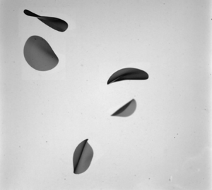
  $500\ \mathrm {\mu }\textrm {m}$ in length. Each voxel is projected onto each image plane. The voxels for which their projections belong to a disc in all images are stored. At the end of this stage the deformed disc is made of a group of voxels. As we aim to reconstruct a surface, voxels which are not at the boundary of the object are discarded. Moreover, if two voxels are projected identically onto an image, the voxel closer to the camera is stored and the farther is discarded. An illustration of the voxel selection is sketched in figure 1(d), and an example of a reconstructed disc from three images is shown in figure 1(e).

Figure 1. (a–c) Typical images with a superposition of the reconstructed disc shown in red dots. (d) Illustration of the reconstruction process with the voxel selection. Here, for simplicity, the axis of the voxel array is aligned with the axes of the cameras. (e) Reconstructed object from the convex hull volume method with the voxel selection detailed in the text. The colour denotes the  $z$ coordinate of the voxel
The convex hull volume method only gives access to the convex envelope of the object and not to its real shape. However, this information is sufficient for determining if a disc is bent. Here, disc deformations are quantified by the moment of inertia tensor  $I$ defined by
 \begin{equation} I_{ij}=\sum_{k=1}^N m_k\left( |r_k|^2\delta_{ij} - x_i^{(k)}x_j^{(k)} \right), \end{equation}
where  $r_k=(x_1^{(k)},x_2^{(k)},x_3^{(k)})$ is the vector connecting the voxel
  $k$ to the centre of mass of the group of voxels and
  $m_k$ is the mass of point
  $k$ which is constant here, so
  $m_k=m$. The shape of the object can be characterised by the three eigenvalues
  $\lambda _1\leqslant \lambda _2\leqslant \lambda _3$. These quantities are extensive, as they depend on the mass of the particle. This prevents an easy comparison of discs having different sizes. To work with intensive quantities, we define two shape factors
  $\lambda _{1}/\lambda _3$ and
  $\lambda _{2}/\lambda _3$ independent of the disc size. These shape factors are not shape specific, meaning that two different objects can have the same shape factors. For instance, a cuboid of dimension
  $d_1=d_2>d_3$ and a cylinder of length
  $L_f$ and radius
  $r_f$ have the same shape factors if
  $3d_3^2/d_1^2=L_f^2/r_f^2-2$. A cube (
 $d_1=d_2=d_3$) and a cylinder of aspect ratio
  $L_f/r_f=\sqrt {5}$ also have the same shape factors. In the plane (
 $\lambda _1/\lambda _3$,
 $\lambda _2/\lambda _3$), three points are remarkable: the point (1/2,1/2) which corresponds to a thin disc, (1,0) to a thin cylinder and (1,1) to a sphere. In figure 2(a) the different shape factors measured for discs made with the silicone R1 (
 $e=190\ \mathrm {\mu }\textrm {m}$ and
  $R=8$ mm) at
  $F_{rot}=19$ Hz are shown. Most of the points stay in the vicinity of the point (0.5,0.5) corresponding to a flat disc. This shows that, in this case, most of the discs are undeformed. There is also a cluster of points in the neighbourhood of the point (0,1) corresponding to a cylinder. This suggests that, at the onset of the transition, deformable discs tend to roll up more than to crumple like a packed paper sheet.

Figure 2. (a) Ratio of the shape factor  $\lambda _2/\lambda _3$ as a function of
  $\lambda _1/\lambda _3$ for all of the reconstructed discs made from silicone R1 (
 $R=8$ mm,
  $e=190\ \mathrm {\mu }\textrm {m}$) at
  $F_{rot}=19\ \textrm {Hz}$. The shaded area is an unreachable zone as
  $\lambda _2>\lambda _1$ by definition. (b) Evolution of the mean shape factor for the same disc at different frequencies. The colour denotes the frequency. The plain line and the dashed line correspond to theoretical prediction; see text for more details. (c) Evolution of the mean shape factor as a function of the turbulent dissipation rate for all the discs (for symbols, see table 2).
To characterise the transition from rigid to flexible disc, we focus on the mean shape factors  $\langle \lambda _{1}\rangle /\langle \lambda _3\rangle$ and
  $\langle \lambda _{2}\rangle /\langle \lambda _3\rangle$, where
  $\langle \cdot \rangle$ is a time and an ensemble average. The evolution of these parameters when the rotation rate
  $F_{rot}$ is varied is shown in figure 2(b) for the same discs as in figure 2(a). One can see that these shape factors are good proxies for the disc deformability as the evolution of
  $\langle \lambda _2\rangle /\langle \lambda _3\rangle$ and
  $\langle \lambda _1\rangle /\langle \lambda _3\rangle$ is monotonic when the rotation rate of the impellers increases, and so when the turbulent dissipation rate
  $\varepsilon$ increases. In the following the disc deformability will be quantified by
  $\langle \lambda _2\rangle /\langle \lambda _3\rangle$ which increases when the deformation of the disc increases. The evolution of this parameter as a function of
  $\varepsilon$ is shown in figure 2(c). As expected, the deformability increases with the turbulent dissipation rate and is higher for discs having a smaller Young's modulus or a smaller aspect ratio
  $\varLambda =e/R$.
4. Modelling
4.1. Disc shape
We will first model the evolution of the disc shape. As shown in figures 2(a) and 2(b), at the onset of the transition, discs tend to wrap and form cylinder like particles. The exact shape of the disc is given by the equation of elasticity
 \begin{equation} \sigma \partial_{tt} r + B \nabla^2\nabla^2 r = \xi, \end{equation}
where  $r$ is the position of a point on the disc,
  $\partial _{tt}$ the second temporal derivative,
  $\sigma =\rho e$ the surface density and
  $B=Ee^3/12(1-\nu )$ the bending modulus of the disc, with
  $\nu \simeq 0.5$ the Poisson coefficient of silicone, and
  $\xi$ the hydrodynamic stress. The disc being freely advected and as no external torque is applied at the boundary, the boundary condition is
  $\kappa (r=R)=0$.
To model the evolution of the shape, we consider a simple solution where a flat disc lies in the  $x$–
$x$– $z$ plane and can only deform in the
  $y$ direction according to
 \begin{equation} y_d(x)=\frac{K_0}{2}x^2\left(1-\frac{x^2}{6x_R^2}\right), \end{equation}
where  $K_0$ is the curvature at the centre of the disc and
  $x_R$ the lateral extension of the disc. For an inextensible disc,
  $x_R$ is defined by the arc length which should be equal to the disc radius
 \begin{equation} R=\int_0^{x_R}\textrm{d}s=\int_0^{x_R}\sqrt{{\textrm{d} x}^2+{\textrm{d} y}^2}=\int_0^{x_R}\sqrt{1+K_0^2x^2\left(1-\frac{x^2}{3x_R^2}\right)^2}\,{\textrm{d} x}. \end{equation}
Representations of a flat and a bent disc are shown in figure 3. The  $(x,y,z)$ axes being the principal axes of the object, the eigenvalues of the moment of inertia of the bent disc are given by
 $$\begin{gather} I_x=\int_{x_R}^{x_R} {\textrm{d} x} \int_0^{\infty} {\textrm{d} y}\int_{{-}z_m}^{z_m}\textrm{d}z ((y-y_G)^2+z^2) \delta\left(y-y_d(x)\right), \end{gather}$$
 $$\begin{gather}I_y=\int_{x_R}^{x_R} {\textrm{d} x} \int_0^{\infty} {\textrm{d} y}\int_{{-}z_m}^{z_m}\textrm{d}z (x^2+z^2) \delta\left(y-y_d(x)\right), \end{gather}$$
 $$\begin{gather}I_z=\int_{x_R}^{x_R} {\textrm{d} x} \int_0^{\infty} {\textrm{d} y}\int_{{-}z_m}^{z_m}\textrm{d}z ((y-y_G)^2+x^2) \delta\left(y-y_d(x)\right), \end{gather}$$
where  $z_m(x)$ is the maximum height of the disc at the position
  $x$ and is given by
 \begin{equation} z_m^2(x)=R^2-\left(\int_0^x\,\textrm{d}s\right)^2, \end{equation}
and  $y_G=3 K_0x_R^2 /20$ is the
  $y$-coordinate of the centre of gravity. The exact expressions of the moments of inertia are relatively tricky to compute analytically. We then compute the evolution of the shape factors numerically for different
  $K_0$, cf. figure 4(a). The theoretical evolution of the bent disc in the
  $(\lambda _1/\lambda _3, \lambda _2/\lambda _3)$ plane is represented by the plain line in figure 2(b). As one can see, the general trend is well captured by this model, but there is an offset between the measurements and the theoretical prediction. Two sources of discrepancy can be identified. First, the number of voxels forming the disc is much smaller than the number of voxels used to compute the theoretical moment of inertia. A second source of error is related to the convex hull volume method. As detailed previously, for voxels projecting onto the same pixel only the voxel closest to the camera is stored. The reconstructed disc is then, in general, not a disc but a partially filled cylinder, as illustrated by figure 1(d). To estimate the order of magnitude of this last source of error, we can compute the shape factor of an object made of touching two coaxial cylinders: one filled of radius
  $R$ and thickness
  $h$, and one empty cylinder of inner/outer radii
  $R_1$ and
  $R$ with the same height
  $h$. Here,
  $h$ is given by the voxel size and we take
  $R_1=R-h$. The evolution of
  $\lambda _2/\lambda _3$ for this object is shown in figure 4(b). The value of the shape factor for
  $h=0$ is equal to the one of a flat disc and increases when
  $h$ is increased. As mentioned previously, the exact value of the offset cannot be determined rigorously and has been considered as a constant free parameter to fit the data. The dashed line in figure 2(b) is obtained by shifting the theoretical prediction for a disc by 0.1 in the vertical direction (
 $\langle \lambda _2\rangle /\langle \lambda _3\rangle$) and 0.01 in the horizontal direction (
 $\langle \lambda _1\rangle /\langle \lambda _3\rangle$). These coefficients will remain fixed in the following sections.

Figure 3. Three-dimensional representation of an undistorted disc  $K_0=0$, (a), and of a bent disc,
  $K_0 R=1$, (b).

Figure 4. (a) Theoretical evolution of the shape factors of a bent disc represented in figure 3 as a function of the normalised curvature  $K_0R$. (b) Evolution of the mean shape factor
  $\langle \lambda _2 \rangle /\langle \lambda _3 \rangle$ for a partially empty cylinder.
Here, the agreement between our model and our measurements suggests that near the transition the disc bend and adopt a U-shape which can be described by (4.2). All the physics of the deformation are then hidden in the parameter  $K_0$, which depends on the disc deformability and the turbulent intensity. The following sections aim to model these dependencies.
4.2. A power budget argument
As shown in figure 4(a), if  $K_0R\lesssim 10^{-2}$ the deformations are weak and the disc can be seen as rigid, whereas if
  $K_0R>10^{-2}$ deformations are important and the disc is indeed flexible. The curvature
  $K_0$ then plays a role similar to the persistence length
  $\ell _p$ for the deformation of worm-like chain polymers. The stiffness of polymers is characterised by the ratio of their length
  $L_p$ to the persistence length
  $\ell _p$, defined by
  $\langle t(s)\cdot t(s+\ell ) \rangle = \textrm {e}^{-\ell /\ell _p}$, where
  $t(s)$ is the tangent vector at the position
  $s$ (Yamakawa Reference Yamakawa1971). If
  $L_p\gg \ell _p$, deformations are important. On the contrary, if
  $L_p\ll \ell _p$, the polymer remains straight and is considered stiff. In polymer theory, the order of magnitude of the persistence length is given by the balance of the thermal energy
  $k_B T$ with the elastic energy
  $\mathcal {E}_{el}\sim EI/\ell _p$, where
  $k_B$ is the Boltzmann constant,
  $T$ the temperature and
  $I$ the area moment of inertia. Brouzet et al. (Reference Brouzet, Verhille and Le Gal2014) draw an analogy between this system and flexible fibres distorted by a turbulent flow. They showed that the energy balance was not able to capture the transition from rigid to flexible fibres. The reason is that the correlation time of turbulence is, in general, of the same order of magnitude as the dynamical time scale of the deformations. Therefore, contrary to polymers, the forcing cannot be modelled by delta correlated noise. The energy budget has then to be replaced by a balance of power. Indeed, the deformation of a fibre in a stationary turbulent flow is an out-of-equilibrium stationary process. The mean elastic energy stored by the fibre
  $\mathcal {E}_{el}$ is then constant and
 \begin{equation} \frac{\textrm{d} \mathcal{E}_{el}}{\textrm{d}t}=P_{inj}-P_{dis}=0, \end{equation}
where  $P_{inj}$ is the power injected by the turbulence and
  $P_{dis}$ is the power dissipated by viscosity. For fibres whose lengths are in the inertial range, deformations are due to eddies of similar sizes. The turbulent power
  $\mathcal {P}_{turb}$ is then given by
  $\mathcal {P}_{turb}\sim \rho _f L_p^3 \varepsilon$. The dissipative term should be proportional to the elastic energy
  $\mathcal {E}_{el}$ stored in the fibre and should depend on the typical time scale of the deformation
  $\tau _{def}$. The ratio of these two terms defines an elastic power
  $\mathcal {P}_{el}$. For fibres, they showed that the time scale of the deformation is given by the relaxation time defined by the ratio of the viscous stress to the bending stress.
Following a similar argument, one can assume that the transition from a rigid to a flexible disc is given by the balance of the turbulent power
 \begin{equation} \mathcal{P}_{turb}\sim \rho_f R^3 \varepsilon, \end{equation}
and the elastic power
 \begin{equation} \mathcal{P}_{el,v}=B \kappa^2 R^2/\tau_{B}, \end{equation}
where  $\tau _{B}$ is the relaxation time scale of the deformation given by the balance of the viscous stress
  $\xi _v$ with the bending stress
  $B\nabla ^2\nabla ^2 r$ in (4.1). From dimensional analysis, at small Reynolds number,
  $\xi _v$ scales as
 \begin{equation} \xi_v \sim \frac{\mu}{R} (u_f-\partial_t r), \end{equation}
where  $u_f$ is the fluid velocity and
  $\mu$ the dynamical viscosity of the fluid. The relaxation time is then
 \begin{equation} \tau_B \sim \mu R^3/B, \end{equation}
and, assuming that at the transition  $\kappa$ can be replaced by
  $1/R$ in (4.10), the elastic power scales as
 \begin{equation} \mathcal{P}_{el,v}\sim \frac{B^2}{\mu \rho_f R^3}. \end{equation}
The balance of power  $\mathcal {P}_{turb}=\mathcal {P}_{el,v}$ defines a critical turbulent dissipation rate
  $\varepsilon _v$
 \begin{equation} \varepsilon_v = \frac{B^2}{\rho_f \mu R^6}. \end{equation}
If this model were able to capture the physics of the deformation, the evolution of the mean shape factors should only depend on the ratio  $\varepsilon /\varepsilon _v$. To compare the theoretical evolution of the shape factor with this prediction one needs to relate the curvature
  $K_0$ to
  $\varepsilon$. Using (4.9), (4.10) and (4.12), which define the turbulent and elastic power, one can show that, near the threshold, the typical curvature
  $\kappa$, and therefore
  $K_0$, should be proportional to
  $\varepsilon ^{1/2}$. The comparison of the theoretical and measured evolution of the mean shape factors as a function of
  $\varepsilon /\varepsilon _v$ is shown in figures 5(a) and 5(b). The dashed line is the best fit of the experimental measurements considering
  $K_0$ as a free parameter. Here, the global trend is well captured by the theoretical prediction. However, the estimation of the threshold with this model is not valid as evidenced by the scattering of the experimental points around the theoretical prediction. In particular, the threshold of the discs having the highest densities (red stars and blue circles) seems to be at least one order of magnitude lower than the model prediction.

Figure 5. Evolution of the mean shape factors  $\langle \lambda _1\rangle /\langle \lambda _3\rangle$ (a) and
  $\langle \lambda _2\rangle /\langle \lambda _3\rangle$ (b) as a function of the normalised turbulent dissipation rate
  $\varepsilon /\varepsilon _v$. The dashed line represents the best fit of an ideal bent disc; see text for more details.
In this model, inertia is always neglected. It is then not surprising that the dependency of the transition on the disc density is not captured for the higher densities. Another model, derived by Rosti et al. (Reference Rosti, Banaei, Brandt and Mazzino2018), considers the density of fibres. The transposition of their model to discs is presented in the following section.
4.3. A temporal argument
The second model used to quantify fibre deformation is based on a temporal argument. If the forcing time scale is smaller than the deformation time scale, deformations are weak as fibres do not have the time to adapt their shapes to the flow. On the contrary, if the forcing time scale is larger than the deformation time scale, the fibre is distorted by the coherent structures of the flow.
As for the model presented in § 4.2, the transposition of this idea to the current study requires an estimation of the deformation time scale of the discs. Two time scales are relevant depending on the influence of particle inertia. The first one is the relaxation time scale, as defined by (4.12). It is used to define the Weissenberg number, which generally quantifies polymer deformations in turbulent flows (Vincenzi et al. Reference Vincenzi, Watanabe, Sankar Ray and Picardo2021). The second one is the resonant frequency, which has been used by Rosti et al. (Reference Rosti, Banaei, Brandt and Mazzino2018) to quantify fibre deformations in the underdamped regime, i.e. when viscous stress is negligible as compared with particle inertia. As shown previously, the relaxation time is independent of the particle density. Therefore, a model solely based on this time scale should not be able to describe our measurements.
The resonant frequency of the disc  $\omega _d$ is given by the equation of elasticity (4.1) by balancing the inertial term
  $\sigma \partial _{tt}r$ and the bending term
  $B\nabla ^2\nabla ^2r$
 \begin{equation} \omega_d^2 = c_\omega \frac{B}{\sigma R^4}, \end{equation}
where  $c_\omega$ is a constant which depends on the excited mode. In the following we will consider the case where
  $c_\omega =1$. When the disc radius
  $R$ is in the inertial range of turbulence, the relevant time scale for the forcing
  $\tau _{turb}$ is the typical time of eddies of similar size
 \begin{equation} \tau_{turb}\sim R/u_R\sim R^{2/3}\varepsilon^{{-}1/3}, \end{equation}
where  $u_R\sim (\varepsilon R)^{1/3}$ is the typical velocity at scale
  $R$. From these two time scales, one can define an inertial Weissenberg number
  $Wi=\omega _d \tau _{turb}$ which should be of order unity at the transition. This defines a critical turbulent dissipation rate
  $\varepsilon _{r}$ above which a disc can be bent
 \begin{equation} \varepsilon_r = \frac{B^{3/2}}{\sigma^{3/2} R^4} . \end{equation}
Contrary to the previous model, this model cannot predict the evolution of the mean curvature  $\kappa$ as a function of
  $\varepsilon$. There was relatively good agreement between the shape of the theoretical prediction and the global trend of the measurement in the previous scaling argument, so we will assume that
  $\kappa \sim \varepsilon ^{1/2}$. Once again,
  $K_0$ will be considered as a free parameter in order to fit the experimental data.
The measurements and the theoretical predictions are compared in figures 6(a) and 6(b). As for the previous case, there is a scattering of the experimental points around the theoretical prediction for both shape factors. The failure of this approach is not surprising as it was derived to describe the transition between two modes of deformation of fibres: the excitation of the first bending mode if  $\omega _d\tau _{turb}\ll 1$ and the deformation dependent upon the coherent structures of the flow if
  $\omega _d\tau _{turb}\gg 1$ (Rosti et al. Reference Rosti, Banaei, Brandt and Mazzino2018). On the contrary, we focus here on the transition from rigid to flexible discs which should occur at smaller
  $\varepsilon$.

Figure 6. Evolution of the mean shape factors  $\langle \lambda _1\rangle /\langle \lambda _3\rangle$ (a) and
  $\langle \lambda _2\rangle /\langle \lambda _3\rangle$ (b) as a function of the normalised turbulent dissipation rate
  $\varepsilon /\varepsilon _r$. The dashed line represents the best fit of an ideal bent disc; see text for more details.
4.4. An inertial power balance argument
In the first model presented in § 4.2, the transition from rigid to flexible discs was modelled using a balance between the turbulent power  $\mathcal {P}_{turb}$ and the elastic power
  $\mathcal {P}_{el}=B\kappa ^2R^2/\tau _{el}$ assuming that the time scale of the deformation
  $\tau _{el}$ was the relaxation time scale, cf. (4.12). In the second model (§ 4.3), we introduce a second time scale for the deformation: the frequency of the first bending mode, cf. (4.15). The relevance of each time scale depends on the importance of the disc inertia in the equation of elasticity (4.1). This is quantified by the ratio of the inertial term
  $\sigma \partial _{tt} r\sim \sigma \omega _f^2\zeta$, where
  $\omega _f$ is the forcing frequency and
  $\zeta$ the typical displacement, to the viscous term
  $\mu \partial _{t}r/R\sim \mu \omega _f\zeta /R$. This ratio defines an elastic Stokes number
  $St_d$
 \begin{equation} St_d \sim \frac{\rho}{\rho_f} \left(\frac{e}{\eta_K}\right)^{4/3} \left(\frac{R}{e}\right)^{1/3}. \end{equation}
Here, we have assumed that the forcing time scale is given by the eddies at the scale of the disc  $\omega _f\sim u_R/R$. In this study,
  $St_d$ varies between 14 and 320. Inertia is then larger than the viscous dissipation and the time scales of the deformation should be given by
  $\omega _d$. This regime corresponds to the underdamped regime investigated by Rosti et al. (Reference Rosti, Banaei, Brandt and Mazzino2018) for fibres. Replacing the relaxation time scale by
  $\omega _d^{-1}$ in the definition of the elastic power leads to
 \begin{equation} \mathcal{P}_{el,w}\sim \frac{B^{3/2}\kappa^2}{\sigma^{1/2}}. \end{equation}
As for the first model, balancing this elastic power with the turbulent power  $\mathcal {P}_{turb}=\rho R^3\varepsilon$, we find that
  $\kappa \sim \varepsilon ^{1/2}$ near the threshold. Moreover, the critical turbulent dissipation rate
  $\varepsilon _w$ can be estimated by defining the threshold of the transition by
  $\kappa \sim 1/R$
 \begin{equation} \varepsilon_w = \frac{B^{3/2}}{\rho_f \sigma^{1/2} R^5}. \end{equation}
The evolution of the shape factors as a function of the normalised turbulent dissipation rate  $\varepsilon /\varepsilon _w$ is shown in figures 7(a) and 7(b). There is now a good agreement between the measurements and the theoretical predictions for all the discs except for the most flexible ones. In that case, deformations probably involved several modes of bending. This cannot be captured by our model and will be discussed in the following section.

Figure 7. Evolution of the mean shape factors  $\langle \lambda _1\rangle /\langle \lambda _3\rangle$ (a) and
  $\langle \lambda _2\rangle /\langle \lambda _3\rangle$ (b) as a function of the normalised turbulent dissipation rate
  $\varepsilon /\varepsilon _r$. The dashed line represents the best fit of an ideal bent disc; see text for more details.
5. Discussion and conclusion
We have presented here an experimental investigation of the deformation of discs within a turbulent flow. The disc deformations have been measured using the convex hull volume method and quantified by the evolution of the shape factors  $\langle \lambda _{1,2}\rangle /\langle \lambda _3 \rangle$, where
  $\lambda _i$ are the eigenvalues of the moment of inertia tensor. We showed that, near the threshold of the transition, the discs adopt a
  $\cup$ shape with a maximum curvature
  $\kappa$ located at the centre and which scales as
  $\kappa \sim \varepsilon ^{1/2}$. The threshold of the transition is given by an equilibrium between the turbulent power
  $\mathcal {P}_{turb}$ and the elastic power
  $\mathcal {P}_{el}$ defined by the ratio of the elastic energy to the time scale of the deformation which is here given by the frequency of the first bending mode. This time scale depends on the elastic Stokes number
  $St_d$, which is relatively large in this study. When
  $St_d\ll 1$, i.e. when
  $e/\eta _K\ll (R/e)^{1/4}$, viscous stress is dominant and the time scale should then be given by the relaxation time
  $\tau _B$, cf. (4.12), as it was for fibres (Brouzet et al. Reference Brouzet, Verhille and Le Gal2014). More studies are needed to understand the influence of the Stokes number on the time scale of the deformations and, hence, on the onset of the deformation.
In our modelling we compare the disc deformation with a folded disc shown in figure 3. For this simple shape the variation of the curvature and of the deflection at the extremity, given by  $y_d(x_R)=5K_0x_R^2/12$, evolves linearly with
  $K_0$ for small deformation, as shown in figure 8(a). The agreement between the experiments and this simple model calls into question the term ‘transition’ we use throughout this paper, which suggests that two different states exist: the rigid and the flexible regimes. In fact, the existence of two different regimes can be seen in the radial extension
  $x_R$ of the disc, cf. figure 8(b), and in the evolution of the shape factors, cf. figure 7. For
  $K_0R \ll 1$,
  $x_R\sim R$ so the shape of the disc is well approximated by a flat disc. For
  $K_0R\gtrsim 1$,
  $x_R< R$, meaning that the radial extension in the
  $x$ direction is smaller than in the
  $z$ direction, cf. figure 3. In this regime, deformations cannot be neglected and should impact the disc dynamics. Moreover, investigation of the fragmentation of brittle fibres shows evidence that the critical length
  $\ell _p$, defined by the balance of power, plays a major role in the fragmentation process (Brouzet et al. Reference Brouzet, Guiné, Dalbe, Favier, Vandenberghe, Villermaux and Verhille2021). Extrapolating this result to brittle discs allows us to define a critical size above which deformations, and the following fragmentation, are important for 2-D objects
 \begin{equation} R_c = \frac{B^{3/10}}{\left(\rho_f \sigma^{1/2} \varepsilon\right)^{1/5}}. \end{equation}
This length scale could be relevant to determine the size of microplastic fragmented in the ocean. Considering a plastic bag made of polyethylene with a Young's modulus of 500 kPa and a thickness of  $80\ \mathrm {\mu }\textrm {m}$ within a turbulent flow with
  $\varepsilon \in [10^{-1};10^2]\ \textrm {m}^{2}\ \textrm {s}^{-3}$, typical during a storm (Gemmrich & Farmer Reference Gemmrich and Farmer2004), the critical size
  $R_c$ varies between 3.2 mm and
  $790\ \mathrm {\mu }\textrm {m}$. These values show that the plastic bag can easily be deformed within the turbulent ocean. Moreover, these length scales are compatible with field measurements where the fragment size distribution exhibits a maximum for microplastic particles around 1 mm (Cózar et al. Reference Cózar2014).

Figure 8. Evolution of the deflection  $y(x_R)=\delta$ (a) and the radial extension
  $x_R$ (b), see (4.3), as functions of the curvature
  $K_0$.
Finally in § 4.3, we claimed that the critical value  $\varepsilon _r$ derived from the temporal argument (
 $Wi=1$) should be larger than
  $\varepsilon _w$. In fact,
  $\varepsilon _r$ characterises a transition where the topology and the dynamics of the deformation are given by the coherent structures of the flow and not by the eigenmode of the disc. To fully validate this claim more measurements are needed. However, we can compare the two thresholds
  $\varepsilon _r$ and
  $\varepsilon _w$
 \begin{equation} \frac{\varepsilon_w}{\varepsilon_r}=\frac{\sigma}{\rho_f R}=\frac{\rho}{\rho_f}\frac{e}{R}. \end{equation}
In the case of the most flexible discs investigated here (purple diamonds), this ratio is of the order of 1/30. As the threshold of the transition from flat to bent disc occurs for  $\varepsilon /\varepsilon _w\sim 3$, cf. figure 7, the second regime of deformation where coherent structures of the flow are responsible of the disc deformation occur then at
  $\varepsilon /\varepsilon _w\gtrsim 90$, as it is the case here, cf. figure 7. In general, when
  $\rho \sim \rho _f$, for 2-D objects where
  $e\ll R$, the transition derived from the temporal argument occurs at higher turbulent dissipation rate
  $\varepsilon$ than the one corresponding to the excitation of the bending mode. When the particle and the carrying fluid have very different densities, like a plastic bag advected in air, this ratio can be of order unity (for a plastic bag with a thickness
  $e=80\ \mathrm {\mu }\textrm {m}$ and of typical size 20 cm
  $\varepsilon _w/\varepsilon _r\sim 2$). In that case, the deformation should directly be driven by the coherent structures of the flow. Further investigation is needed to validate this point.
Funding
This work was carried out in the framework of FlexFiT Project (ANR-17-CE30-0005-01) funded by the French National Research Agency (ANR).
Declaration of interests
The author reports no conflict of interest.


