2. Two-dimensional stratified flow

Consider a uniformly stratified inviscid, diffusionless fluid which in its undisturbed state has constant buoyancy frequency $N$. Introduce Cartesian axes $Ox'yz$ fixed in the fluid with $Oz$ vertical and take the motion to be two-dimensional in the sense that the flow is independent of the coordinate $y$, being the same in all vertical slices $y=$ constant with all quantities treated below as two-dimensional but corresponding to three-dimensional quantities taken per unit width in the $y$-direction. Let the fluid be disturbed by a circular LC-dipole of radius $a$ propagating in the $Ox'$ direction at speed $U$, such that the inverse Froude number, the ratio of the vortex scale to the scale of internal waves that can stand behind the propagating vortex, $\epsilon _N = Na/U$, is small (figure 1a). Now consider the leading-order flow in the limit $\epsilon _N\to 0$ so that on the scale of the vortex the leading-order flow is nonlinear but unaffected by stratification. On the scale of the internal wave wake the vortex appears as a forcing region of area $\epsilon _N^{2}$ and so is governed by linear dynamics. The internal wave pressure field acts over a length of order $\epsilon _N$ to exert a drag of order $\epsilon _N^{3}$ on the vortex. This weak drag causes the vortex to be modified over a time scale $\epsilon _N^{3}a/U$, long compared to the advection time $a/U$. As a modelling hypothesis it will be supposed that the response of the vortex to this drag is to evolve so as to remain an LC dipole but with radius and speed varying slowly in time. The internal wave wake is set up in times of order $a/U$ and so can be taken as quasi-steady during the vortex evolution. The solution requires three components described briefly below: the dipole energy (§ 2.2), the wave drag (§ 2.3) and an appropriate vortex centre (§ 2.4).

2.1. The governing equations

Let the velocity relative to the fixed axes $Ox'yz$ be $\boldsymbol {u}=u\boldsymbol {\hat {x}'} + w\boldsymbol {\hat {z}}$ and buoyancy acceleration be $b$. For two-dimensional flows in an otherwise static, stably stratified flow of buoyancy frequency $N$, the equations of motion can be written in coordinates moving at the vortex speed $U$ as

(2.1a)\begin{gather} (\partial_t - U\partial_x)u +uu_x+wu_z ={-}(1/\rho)p_x, \end{gather}

(2.1b)\begin{gather}(\partial_t - U\partial_x)w+uw_x+ww_z - b ={-}(1/\rho)p_z, \end{gather}

(2.1c)\begin{gather}(\partial_t - U\partial_x)b+ub_x+wb_z + N^{2} w = 0, \end{gather}

(2.1d)\begin{gather}u_x+w_z = 0, \end{gather}

where $\rho$ is a constant reference density and $x = x' - \int ^{t} U(t') \,{\textrm {d}}t'$. This system gives an energy conservation equation in the form

(2.2a,b)\begin{equation} \partial_t E_b + \boldsymbol{\nabla} \boldsymbol{\cdot} [E_b({-}U\boldsymbol{\hat{x}}+{\boldsymbol{u}})+p{\boldsymbol{u}}] = 0, \quad E_b =\tfrac{1}{2}\rho(u^{2}+w^{2})+\rho b^{2}/N^{2}. \end{equation}

Introducing the streamfunction $\psi$, defined by $(u,w)=(\psi _z,-\psi _x)$, and eliminating the pressure then gives for steady flow,

(2.3a)\begin{gather} \partial({-}Uz+\psi,\eta) - b_x =0, \end{gather}

(2.3b)\begin{gather}\partial({-}Uz+\psi,b+N^{2}z) =0, \end{gather}

where $\eta =\nabla ^{2}\psi$ is the $y$-component of vorticity and $\partial (.,.)$ denotes the Jacobian. Simple nonlinear solutions of (2.3) follow by looking for Long's model solutions (Long Reference Long1955) where the total density $b+N^{2}z$ is a linear function of the total streamfunction $-Uz+\psi$, i.e. $b+N^{2}z = \alpha (-Uz+\psi )$, for some $\alpha$. For streamlines originating upstream, where $b$ and $\psi$ vanish, this form requires that $\alpha =-N^{2}/U$ but within the vortex $\alpha$ is arbitrary. Then (2.3a) can be written

(2.4)\begin{equation} \partial({-}Uz+\psi,\eta -\alpha z)=0. \end{equation}

A simple nonlinear solution is again given by choosing $\eta - \alpha z$ to be a linear function of $-Uz+\psi$, i.e. $\eta - \alpha z = \gamma (-Uz+\psi )$, for some $\gamma$. For streamlines originating upstream this form requires that $\alpha = U\gamma$ but within the vortex $\gamma$ is arbitrary. The governing equation outside the vortex thus becomes

(2.5a)\begin{gather} \nabla^{2} \psi + \kappa^{2} \psi = 0, \end{gather}

(2.5b)\begin{gather}b ={-} N^{2}\psi/U, \end{gather}

where $\kappa =N/U$ is the wavenumber of the standing internal wave wake. Multiplying (2.5a) by $\psi$ and integrating over the region exterior to the vortex shows that the energy in the internal wave wake is equipartitioned between kinetic and potential energy as expected,

(2.6)\begin{equation} \int (u^{2}+w^{2}) = \int (\psi_x^{2}+\psi_z^{2}) = \kappa^{2} \int \psi^{2} = \int b^{2}/N^{2} . \end{equation}

Now suppose that relationship (2.5b) between the density and streamfunction continues to hold within the vortex (so in the absence of stratification the perturbation density vanishes). Then the governing equation inside the vortex can be written

(2.7)\begin{equation} \nabla^{2} \psi + K^{2} \psi = U(K^{2}-\kappa^{2})z, \quad b={-} N^{2}\psi/U, \end{equation}

where $K$ is the internal wavenumber of the vortex. For $K\neq \kappa$ the energy of the vortex does not satisfy (2.6) and is not equipartitioned between kinetic and potential energy. Larichev & Reznik (Reference Larichev and Reznik1976) and Flierl (Reference Flierl1987) derive system (2.5), (2.7) with $\kappa ^{2}$ replaced by $-(\beta /U)$ as the governing equation for eastward propagating dipolar vortices, modons, in a barotropic rigid-lid ocean under the $\beta$-plane approximation and give solutions for circular dipoles surrounded by an exponentially decaying disturbance field. This form of solution requires the modon speed $U$ to be positive so as to lie outside the range of Rossby wave phase speeds. Westward propagating modons, $U<0$, have a speed that coincides with a Rossby wave phase speed. This permits standing Rossby lee-wave wakes that remove momentum and energy from the modon and FH quantify the subsequent modon decay. As there is no preferred horizontal direction for internal waves the dipoles in the stratified flow here decay irrespective of their direction of propagation.

2.2. The LC dipole

In the absence of background stratification ($\kappa =0$) system (2.1) reduces to the Euler equations. Equations (2.5), (2.7) have the LC-dipole solution (Meleshko & van Heijst Reference Meleshko and van Heijst1994),

(2.8)\begin{equation} \psi= \begin{cases} Uz + C \operatorname{{\mathrm{J}}_1}(Kr)z/r, & r<a \\ Ua^{2}z/r^{2}, & r>a, \end{cases} \end{equation}

where $r=(x^{2}+z^{2})^{1/2}$, and the dipole boundary is the circle $r=a$. The smallest wavenumber $K$ satisfying the no-normal-flow condition, $-Uz+\psi =0$ on $r=a$, i.e. $\operatorname {{\mathrm {J}}_1}(Ka)=0$, is given by $Ka = \gamma$ where $\gamma$ is the first positive root of $\operatorname {{\mathrm {J}}_1}$ so $\gamma \approx 3.8317$. Once $a$ is determined $K$ is known. Continuity of tangential velocity at the dipole boundary gives $C=-2U/K\operatorname {{\mathrm {J}}_0}(Ka)$. The flow outside the dipole can be written

(2.9)\begin{equation} \psi = Ua^{2} \frac{\partial\phantom{x}}{\partial x}[\operatorname{arctan}(x/z)] , \quad r>a. \end{equation}

Along the line $z=0^{+}$, (2.9) gives

(2.10)\begin{equation} \psi = \frac{\rm \pi}{2} Ua^{2} \frac{\partial\phantom{z}}{\partial x}\operatorname{sgn} x = {\rm \pi}Ua^{2}\delta(x) , \quad z=0^{+}, \end{equation}

showing that the velocity field in $r>a$ is precisely that of an irrotational source doublet of strength $2{\rm \pi} \rho Ua^{2}$ at the origin directed in the positive-$x$ direction.

The impulse of the dipole is

(2.11)\begin{equation} \mu ={-}\rho\int z\eta = 2{\rm \pi}\rho Ua^{2}, \end{equation}

where the integral is taken over the compact support of $\eta$ (here the disc $r<a$), and matches the doublet strength. The energy associated with the dipole is simply the kinetic energy

(2.12)\begin{equation} E ={-}\tfrac{1}{2}\rho\int \psi\eta = 2{\rm \pi}\rho a^{2} U^{2}=U\mu. \end{equation}

Under the hypothesis that the dipole remains within the LC-dipole family as it evolves, (2.2a,b) shows that the dipole potential energy remains a small perturbation to the total energy density of the dipole for sufficiently small $\kappa$.

2.3. The internal wave wake

The propagating dipole appears in the outer field as a source doublet of strength $\mu$ propagating to the right at speed $U$. The wave drag on the dipole is weak and so over times of the order of the advection time, the time taken for the internal wave wake to be established in the neighbourhood of the dipole, the dipole radius and speed are unaltered. The wave field can be thus taken as steady in the frame moving with the dipole. The nonlinear terms are negligible in (2.1), the material derivative is simply $-U\partial _x$, and the governing equations again reduce to (2.5) showing, incidentally, that the wave field derived here satisfies the full nonlinear steady equations. For sufficiently small $x$, $z$ the buoyancy term in (2.5) is negligible so the inner region of the internal wave field is irrotational, joining smoothly to the irrotational outer part of the LC-dipole solution (2.8). The linear solution for horizontally propagating dipoles in a weakly stably stratified flow has been solved in both two and three dimensions by Gorodtsov & Teodorovich (Reference Gorodtsov and Teodorovich1983). The solution for two dimensional flow is summarised here and that for three dimensions is simply quoted where needed in § 5. Equation (2.5) is solved in $z>0$ subject to the boundary condition (2.10) and the solution smoothly extended into $z<0$ by taking $\psi$ to be odd in $z$. This gives the Fourier transform solution,

(2.13a)\begin{equation} \psi(x,z) =\frac{1}{2{\rm \pi}}\int_{-\infty}^{\infty}\hat{\psi}(k,z)\exp({\textrm{i}}kx)\,\textrm{d}k, \end{equation}

where

(2.13b)\begin{equation} \hat{\psi}(k,z) = {\rm \pi}U a^{2} \begin{cases} \exp[-(k^{2}-\kappa^{2})^{1/2}\; z], & |k|>\kappa \\ \exp[-{\textrm{i}}\operatorname{sgn}(k)(\kappa^{2}-k^{2})^{1/2}\; z], & |k|<\kappa, \end{cases} \end{equation}

and the sign in the second exponential has been chosen to give upward group velocity.

The drag $D$ exerted on a material surface at height $z$ is given by the component of the pressure force in the negative-$x$ direction. Let $\zeta (x,z_0)$ be the displacement from height $z_0$ of a particle originally at height $z=z_0$ far upstream. Then

(2.14)\begin{equation} D ={-}\int_{-\infty}^{\infty} p\zeta_x \,\textrm{d}\kern0.06em x. \end{equation}

This force is positive, corresponding to a drag on the material surface, when there is a positive upward flux of $x$-momentum. Substituting $w=-U\zeta _x$ from the definition of $\zeta$ and $p=\rho Uu$ from (2.1a) gives

(2.15a)\begin{align} D &= \rho\int_{-\infty}^{\infty} uw \,\textrm{d}\kern0.06em x ={-}\rho\int_{-\infty}^{\infty} \psi_x \psi_z \,\textrm{d}\kern0.06em x ={-}\frac{\rho}{2{\rm \pi}} \int_{-\infty}^{\infty} \widehat{\psi_x}\widehat{\psi_z}^{*} \,\textrm{d}k \end{align}

(2.15b)\begin{align} &={-} \tfrac{1}{2}{\rm \pi}\rho U^{2}a^{4}\left\{\int_{|k|>\kappa} {\textrm{i}}k (k^{2}-\kappa^{2})^{1/2}\exp[{-}2(k^{2}-\kappa^{2})^{1/2}\; z] \,\textrm{d}k\right.\notag\\ &\quad +\left. \int_{-\kappa}^{\kappa} -|k|(\kappa^{2}-k^{2})^{1/2} \,\textrm{d}k\right\} \end{align}

(2.15c)\begin{align} &={-}\tfrac{1}{3}{\rm \pi}\rho U^{2}a^{4}[(\kappa^{2}-k^{2})^{3/2}]_0^{\kappa} = \tfrac{1}{3}{\rm \pi} \rho U^{2}a^{4}\kappa^{3}. \end{align}

Here, (2.15a) follows from Plancherel's theorem and $^{*}$ denotes complex conjugate. The first integrand in (2.15b) is odd in $k$ so the integral vanishes, as expected for evanescent waves, and the second integrand is even giving (2.15c). Waves are radiated both upwards and downwards from the dipole and so the total drag on the dipole is twice that given by (2.15c).

The vertical energy flux is given by the flux of pressure, from (2.2a,b),

(2.16)\begin{equation} F = \int_{-\infty}^{\infty} wp \,\textrm{d}\kern0.06em x = \int_{-\infty}^{\infty} ({-}U \zeta_x) p \,\textrm{d}\kern0.06em x = UD, \end{equation}

the work done by the drag force.

2.4. The vortex centre

As the flow evolves, dipole fluid escapes the boundary of the dipole, in particular from the neighbourhood of the rear stagnation point. The central regions of the vortices comprising the dipole maintain their integrity and so we follow FH and consider the vorticity contained within these regions, defining the instantaneous vortex centre at a given time as the point within the vortex in $z>0$ where the total streamfunction, $\varPsi =-Uz+\psi$, at that time attains its maximum. Consider a total streamline sufficiently close to the vortex centre that it is closed. Integrating the vorticity over the region enclosed by this streamline gives, from (2.1a) and (2.1b),

(2.17)\begin{equation} \int\eta_t\,\textrm{d}\kern0.06em x\,{\textrm{d}}z +\oint\eta({\boldsymbol{u}}.{\boldsymbol{\hat{n}}})\,{\textrm{d}}s = \int b_x \,\textrm{d}\kern0.06em x\,{\textrm{d}}z = \oint b \,{\textrm{d}}z, \end{equation}

where ${\textrm {d}}s$ is the element of length along the streamline. Integrating the buoyancy over the same region gives, from (2.1c),

(2.18)\begin{equation} \int b_t\,\textrm{d}\kern0.06em x\,{\textrm{d}}z +\oint(b+N^{2} z)({\boldsymbol{u}}{\boldsymbol{\cdot}}{\boldsymbol{\hat{n}}})\,{\textrm{d}}s = 0. \end{equation}

As the velocity normal to the streamline is zero, the line integral on the left sides of (2.17) and (2.18) vanish. Now allow the streamline value to increase towards the maximum so that the integration area converges on the vortex centre. Provided the maximum buoyancy perturbation at times $t>0$ lies at the vortex centre, as it does initially, then the buoyancy terms on the right side of (2.17) vanish faster than the vorticity term on the left to give in the limit that $\eta _t$ vanishes at the vortex centre: the instantaneous rate of change of the vorticity at the vortex centre is zero. The numerical simulations in §§ 3, 4 below confirm that the vorticity at the vortex centre, denoted herein by $\eta _c$ and described for brevity as the centre vorticity, remains approximately constant throughout the evolution. Similarly, (2.18) shows that the perturbation buoyancy at the vortex centre, denoted herein by $b_c$ and described as the centre buoyancy, is constant throughout the evolution, again borne out by the numerical integrations of § 4.

3. Modon decay through Rossby wave radiation

Before considering the slow evolution of the stratified flow it is useful to relate the analysis of § 2 to that for the decay of modons due to Rossby wave radiation described by FH. The $\beta$-plane approximation consists of taking Cartesian axes $Oxy$ in a horizontal plane with $Oy$ northwards, corresponding velocity components $(u,v)$, streamfunction $\psi$ such that $(u,v) = (-\psi _x,\psi _y)$ and $\beta$ as the local poleward gradient of the vertical component of the Earth's rotation (figure 1b). This gives the quasi-geostrophic potential vorticity equation in a frame moving at speed $U$ to the west, as in FH, as

(3.1)\begin{equation} (\partial_t - U\partial_x)\nabla^{2}\psi +\partial(\psi,\nabla^{2}\psi) + \beta\psi_x = 0. \end{equation}

Equation (3.1) has the same dynamics as that in §2 on setting $\kappa =(-\beta /U)^{1/2}$ for $U<0$. The drag computation in § 2.3 applies directly to give the same expression (2.15c) for the total drag due to Rossby wave radiation and (2.16) for the work done by the wave field: the wave drag method of § 2 gives the same results as the adjoint method of FH.

Equating the rate of change of dipole impulse to the drag force acting on the dipole gives the slow evolution equation, taking into account that $U<0$,

(3.2)\begin{equation} \frac{{\textrm{d}} \mu}{{\textrm{d}}t} ={-}2D, \quad \text{i.e. }\frac{{\textrm{d}} \phantom{t}}{{\textrm{d}}t}(2{\rm \pi} U a^{2}) ={-}\frac{2}{3}{\rm \pi} U^{2}a^{4} \kappa^{3} . \end{equation}

Similarly, balancing the rate of change of vortex energy against the work done by the wave field gives

(3.3)\begin{equation} \frac{{\textrm{d}}E}{{\textrm{d}}t} ={-}2F={-}2UD, \quad \text{i.e. }\frac{{\textrm{d}} \phantom{t}}{{\textrm{d}}t}(2{\rm \pi} U^{2} a^{2}) ={-}\frac{2}{3}{\rm \pi} U^{3} a^{4} \kappa^{3}. \end{equation}

Equations (3.2) and (3.3) combine to require that $U$ remains constant and so

(3.4a,b)\begin{equation} a =a_0(1 + \tfrac{1}{3}\epsilon^{3} |U_0|t/a_0)^{{-}1/2}, \quad \epsilon=\epsilon_{\beta 0}=(-\beta a_0^{2}/U_0)^{1/2}, \end{equation}

where $a_0$ and $U_0$ are the initial values of $a$ and $U$. This is the same result that FH obtain by combining energy conservation with enstrophy conservation. They point out that the peak vorticity within the modon is proportional to $U/a$ and so would increase as the modon shrank, violating Lagrangian conservation of peak vorticity. FH note also that streamers of vorticity are shed from the rear of the dipole, consistent with the instability described by Brion et al. (Reference Brion, Sipp and Jacquin2014), and so it is reasonable to expect that dipole enstrophy is not conserved. Enforcing the conservation of centre vorticity, defined as in § 2.4 is equivalent to requiring that $U/a$ remains constant throughout the evolution. Requiring $U/a$ to remain equal to its initial value while relaxing conservation of enstrophy or, equivalently, the drag–modon impulse balance (3.2), and retaining the work–modon energy balance (3.3), gives the decay rate

(3.5)\begin{equation} a_1(t) =a_0(1 + \tfrac{1}{8}\epsilon^{3} |U_0|t/a_0)^{{-}2/3}. \end{equation}

FH present numerical integrations that strongly support the determination through conservation of centre vorticity. The agreement of the decay rate of various quantities with (3.5) is excellent, particularly in the relevant range of small $\beta$, even though the accompanying wave field seems not to take precisely the asymptotic form. This deviation and the large fluctuations at larger $\beta$ appear to be due to the necessarily finite size of the computational domain. To test this hypothesis equation (3.1) was discretised spectrally using Fourier series on a doubly periodic domain as in FH, but with twice the resolution and four times the domain size ($2048 \times 2048$ points on a grid of size $102.4 \times 102.4$ initialised with an LC-dipole vortex of radius one and speed one) and integrated using the Dedalus package (Burns et al. Reference Burns, Vasil, Oishi, Lecoanet and Brown2020) with a time step of $2 \times 10^{-3}$ and hyperdiffusion included to absorb the downscale enstrophy cascade and ensure numerical stability. The total energy in the domain was conserved to within 1 % over 25 time units for all $\beta$ considered and the centre vorticity to within 5 %. The position of the maximum streamfunction value, $\psi _c(t)$, i.e. the vortex centre, is known accurately at each time step and so the instantaneous speed $U(t)$ can be obtained by differencing the $x$-coordinate of the vortex centre. The instantaneous dipole radius $a(t)$ is more difficult to measure directly. The assumption that the dipole evolves to remain an LC dipole means, however, from (2.8), that

(3.6)\begin{equation} \psi_c(t) = P a(t)U(t), \end{equation}

for some constant $P$. By direct evaluation of the maximum of (2.8), FH show that $P\approx 1.3$ and so $a(t)$ follows from (3.6). The initial dipole adjusts rapidly at early times altering slightly both the initial speed and radius of the modon. We follow FH and evaluate $a_0$ and $U_0$ from the flow field at some time $t=t_0$ after this initial adjustment. These values then determine $\epsilon$ through (3.4a,b), which thus differs slightly from $\beta ^{1/2}$. For definiteness the integrations are labelled by the value of $\beta$.

Figure 2(a) compares the present results for the maximum value of the streamfunction within the modon, the streamfunction value at the vortex centre as defined in § 2.4, with those of FH showing that decreasing the effect of westward-radiated waves re-entering from the eastern boundary, and decreasing wave reflection at the zonal boundaries, due to spatial periodicity, suppresses the fluctuations present on the smaller computational domain. Figure 2(b) shows the decay of modon energy $E$, calculated here as the kinetic energy within a circle of radius $a(t)$ about the translating origin of the dipole. The small $\beta$ results capture the qualitative behaviour even for $\beta =1$ where the modon has lost almost 80 % of its energy by $t=25$. The values for the determination for $a_0$ and $U_0$ are $t_0=1$ in (a) and $t_0=5$ in (b) as the streamfunction appears to fall into its asymptotic behaviour sooner. The values plotted have been normalised by their value at $t=t_0$.

Figure 2. (a) The normalised maximum value of streamfunction within the quasigeostrophic modon: the streamfunction value at the vortex centre, $\psi _c$, and (b) the normalised modon energy, $E$, as functions of time, $t$ for the background vorticity gradients $\beta$ listed in the legend. The solid lines show the present computations, the dashed lines the computations of FH and the dotted lines the analytical predictions.

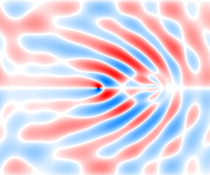
Figure 3(a) shows the wave field at time $t=25$ for $\beta =0.4$ in an inertial frame propagating to the west at unit speed. The initial modon position is marked by ‘$+$’ (and thus is at $X=x'+t=25$ at $t=25$) and the current position by ‘$+$, green’. The wake behind the modon is established between the initial and current modon positions as the modon moves away. Slowly propagating transient waves can be seen originating from the neighbourhood of the initial modon position. As noted by FH, the modon initially accelerates through the $\beta$-effect to move slightly faster than unity but then slows due to wave drag and so by $t=25$ lies just in $X<0$. The wave field has the expected asymptotic form with no clear signature of boundary effects. These features of the solution can be seen more clearly in the movie (Movie 1) of the temporal development of $\psi$, included as supplementary material available at https://doi.org/10.1017/jfm.2021.298. Figure 3(b) shows the vorticity expelled from the rear of the modon as expected from the LC-dipole stability analysis of Brion et al. (Reference Brion, Sipp and Jacquin2014) and from the viscous LC-dipole computations of Nielsen & Rasmussen (Reference Nielsen and Rasmussen1997).

Figure 3. (a) The streamfunction $\psi$ in the horizontal $\beta$-plane forced by a westward propagating quasigeostrophic modon for $\beta = 0.4$ at time $t = 25$. The modon, marked by ‘$+$’, green, moves west from an initial position marked with ‘$+$’, generating the Rossby wave wake. (b) The relative vorticity $\nabla ^{2} \psi$ for $\beta = 0.8$ at $t = 15$, showing vorticity escaping from the rear of the modon.

4. The slow evolution of the stratified flow

The equations corresponding to (3.2) and (3.3) for stratified flow, where $\kappa =N/U$ are the impulse-drag equation

(4.1)\begin{equation} \frac{{\textrm{d}} \phantom{t}}{{\textrm{d}}t}(Ua^{2}) ={-}N^{3}a^{4}/3U, \end{equation}

and the energy-work equation

(4.2)\begin{equation} \frac{{\textrm{d}} \phantom{t}}{{\textrm{d}}t}(U^{2}a^{2}) ={-}N^{3}a^{4}/3. \end{equation}

Again, (4.1) and (4.2) combine to require that $U$ remains constant, giving (3.4a,b) with here $\epsilon =\epsilon _{N0}=Na_0/U_0$, and so contradicting the conservation of centre vorticity of § 2.4. Relaxing the dipole impulse equation (4.1) while requiring the centre vorticity to be conserved, i.e. $U/a$ to remain constant, and the energy equation (4.2) to hold, gives

(4.3)\begin{equation} a_1(t) =a_0\exp(-\tfrac{1}{12}\epsilon_N^{3} |U_0|t/a_0). \end{equation}

The decay rate is exponential here in contrast to the slower algebraic decay rate for the $\beta$-plane modon because of the different power of $U$ in the definition of $\kappa$. The conservation of centre vorticity also implies that the instantaneous value of the inverse Froude number, $\epsilon _N=\kappa a =Na/U$, remains equal to its initial value, $\epsilon _{N0}$, in contrast to the $\beta$-plane modon where the instantaneous value of $\epsilon _\beta$ slowly decreases with time, as $a^{1/2}$, and so the flow becomes progressively less nonlinear. As expected from § 2 the decay time scale is of order $\epsilon ^{-3}$ times the advection time scale.

Equations (2.1) in streamfunction–vorticity form, i.e. the unsteady version of (2.3), were integrated using the code of § 3, including the additional buoyancy field, with the initial condition for the vorticity taken to be an LC dipole, the initial streamfunction obtained from the vorticity by inverting the periodic Laplacian, and the initial buoyancy to be given by (2.5b) so as to be continuous and have continuous normal derivative at $r=a$. The flow pattern developed more slowly than on the $\beta$-plane and so the equations were integrated to $t=50$, with the total energy again conserved to within 1 % over all integrations. The dipoles again evolve slightly but rapidly initially and so $a_0$ and $U_0$ are computed at time $t=t_0$ after this initial evolution with the integrations labelled by the value of $N$.

Figure 4 shows the wave field for $N=0.4$ at times $t=30$ and $t=50$ in an inertial frame propagating to the right at unit speed. The initial dipole position is marked by ‘$+$’ (and thus is at $X=x'-t=-30$ at $t=30$ and at $X= -50$ at $t=50$) and the current position by ‘$+$, green’. As for the $\beta$-plane modon of § 3, the wake behind the dipole is set up between the initial and current dipole positions as the dipole moves away; slowly propagating transient waves can be seen originating from the neighbourhood of the initial modon position; and the dipole initially accelerates, here through buoyancy effects, to move slightly faster than unity but then slows due to wave drag and so lies just in $X>0$ at $t=30,50$. The wave fields are well developed, particularly in the neighbourhood of the dipole, boundary effects are negligible, and the wavelength of the disturbance remains constant with time, as expected. These features can be seen more clearly in the movie (Movie 2) of the temporal development of $\psi$ and $b$, included as supplementary material.

Figure 4. The streamfunction $\psi$ for a rightward propagating dipole in the vertical-slice stratified model for $N = 0.4$ at times (a) $t = 30$, (b) $t = 50$. The dipole, marked by ‘$+$’, green, moves to the right from an initial position marked with ‘$+$’, generating the internal wave wake.

The model here assumes that throughout the evolution the dipole remains an LC dipole, although with varying speed and radius, and that the streamfunction and buoyancy are linearly related. Figure 5 tests these relations at time $t=30$ for $N=0.3$ for the $4\times 10^{6}$ computational points. Figure 5(a) gives a scatter plot of the vorticity $H = (N^{2}/U) z +\nabla ^{2}\psi$ as a function of the total streamfunction $\varPsi =-Uz+\psi$ over the whole flow field and figure 5(b) gives a detail of figure 5(a) in the neighbourhood of the dipole. From (2.5a) and (2.7) the points outside the dipole should lie along a line through the origin with slope $\kappa ^{2}$ and points inside the dipole along a line with slope $K^{2}-\kappa ^{2}$, shown dashed in figure 5(a,b). The closeness of the computed values even at large times shows that the dipole remains close to an LC dipole. A scatter plot of the total density against the total streamfunction (not shown here) shows that these quantities are very closely linearly related, satisfying (2.3b) closely. A more stringent test is shown in figure 5(c) where the perturbation buoyancy $b$ is plotted as a function of the perturbation streamfunction $\psi$ over the whole flow field. The general behaviour accords with the relations (2.5b) and (2.7), with the slope of the theoretical relations reproduced accurately. The blue points correspond to computational points lying outside the dipole and lie accurately along the line of (2.5b). The red points are points lying within the dipole. They show a slightly steeper slope near the geometric centre of the dipole at the co-moving-coordinate origin and a small offset over the majority of the dipole. The points near the ends of the red groups correspond to computational points near the vortex centre. This behaviour cannot be captured by the model presented here but appears to be sufficiently small that it does not alter the qualitative behaviour of the flow. This will be discussed briefly in § 7. The green points are computational points near the dipole boundary affected by the computational hyperdiffusion which smooths otherwise discontinuous higher gradients there.

Figure 5. Scatter plots showing the functional relations in the flow at time $t=30$ for buoyancy $N=0.4$. (a) The total vorticity $H = (N^{2}/U) z +\nabla ^{2}\psi$ as a function of the total streamfunction $\varPsi =-Uz+\psi$ over the whole flow field. (b) A detail of part (a) in the neighbourhood of the dipole. (c) The perturbation buoyancy $b$ as a function of the perturbation streamfunction $\psi$ over the whole flow field. The dashed lines in each part give the theoretical relations discussed in the text.

Figure 6 shows the centre vorticity $\eta _c$ and the centre perturbation buoyancy $b_c$ as functions of time $t$ for different strengths of the background buoyancy gradient, $N$. The values are normalised on their value at $t=t_0$ where here $t_0=10$, reflecting the longer time required for the stratified dipole to adjust to its asymptotic form. For small $N$, $\eta _c$ is closely constant and even for $N=0.4$, $\eta _c$ decreases only by approximately 1.5 % over the integration. The centre perturbation buoyancy, $b_c$, remains within 3 % of its value at $t=t_0$ provided $N\leq 0.3$. The buoyancy fluctuations for larger $N$ appear related to stirring at the vortex centre, discussed briefly in § 7. Figure 7 shows the streamfunction $\psi _{c}$ at the vortex centre and the dipole energy $E$ during the dipole evolution and figure 8(a) the dipole impulse $\mu$, normalised by their values at $t=t_0 =10$. The dipole model results appear to capture the decay here with comparable accuracy to § 3 even over the longer integration time.

Figure 6. The normalised maximum value of (a) the centre vorticity, $\eta _{c}$, and (b) the centre perturbation buoyancy, $b_{c}$, as functions of time, $t$ for the values of the background buoyancy frequency, $N$, listed in the legend.

Figure 7. Normalised values of (a) the maximum value of the streamfunction $\psi _{c}$ at the vortex centre and (b) the dipole energy $E$ as functions of time $t$ for the values of the buoyancy frequency $N$ listed in the legend. The axes are log–linear. Solid lines give the values from the numerical integrations, dotted straight lines those from the dipole theory and dashed straight lines the values from the cylindrical approximation.

Figure 8. (a) As in figure 7 but for the dipole impulse $\mu$. (b) The relative vorticity $\eta =\nabla ^{2} \psi$ in a vertical $(x,z)$ slice for $N=0.5$ at time $t = 15$, showing vorticity escaping from the rear of the dipole.

Gorodtsov & Teodorovich (Reference Gorodtsov and Teodorovich1983) point out that approximating a finite body by a dipole overestimates the drag by including finite contributions from arbitrarily large wavenumbers which are not forced by the body. By approximating a cylinder of radius $a$ by a distribution of sources Gorodtsov & Teodorovich (Reference Gorodtsov and Teodorovich1983) obtain the drag formula, in the notation of § 2.3,

(4.4)\begin{equation} D_C = (8/3){\rm \pi}\rho U^{2} a^{2} \kappa [\operatorname{{\mathrm{J}}_1}(\kappa a)]^{2}, \end{equation}

which they argue is a more accurate estimate of the wave drag as it takes into account the finite size of the forcing region. Substituting $UD_C$ for the work done by the vortex on the fluid in the work-energy equation and imposing conservation of centre vorticity then gives the modified decay formula

(4.5)\begin{equation} a_2(t) =a_0\exp(-\tfrac{1}{3}\epsilon_N [\operatorname{{\mathrm{J}}_1}(\epsilon_N)]^{2} |U_0|t/a_0). \end{equation}

Expression (4.5) reduces to (4.3) in the limit $\epsilon _N\to 0$ and is not correct to any higher order in $\epsilon _N$ than (4.3). To assess whether accounting for the finite vortex size through this cylindrical approximation gives a more accurate model than the dipole model at small but finite $\epsilon _N$ the values of $\psi _c$, $E$ and $\mu$ derived from (3.5) are included in figures 7 and 8(a) as dashed lines. The cylindrical approximation gives a slower decay as expected but the effect for these values of $N$ is negligible compared with the effect of unavoidable small variations in the estimation of $a_0$ and $U_0$ and so finite size effects are not the leading-order omitted effect for stratified dipoles. The same argument applies to the modon decay of § 3 but since the instantaneous inverse Froude number, $\epsilon _\beta =\kappa a = (-\beta a^{2}/U)^{1/2}$, decreases during the evolution the simple form of solution (3.5) is lost. Approximating the Bessel function in (4.4) by its first two terms gives the radius decay, with the first correction, as

(4.6a,b)\begin{equation} a_2(t) = a_0 \tau[1 + \tfrac{3}{8}\epsilon_{\beta 0}^{2}(1-\tau^{2})], \quad \tau = (1 + \tfrac{1}{8}\epsilon_{\beta 0}^{3} |U_0|t/a_0)^{{-}2/3}. \end{equation}

As for (4.5), (4.6a,b) reduces to (3.5) in the limit $\epsilon _{\beta 0}\to 0$ and is not correct to any higher order in $\epsilon _{\beta 0}$ than (3.5). Comparison with the dipole model (not plotted here) show again that finite size effects are not the leading-order omitted effect for $\beta$-plane modons.

Figure 8(b) shows the relative vorticity $\eta =\nabla ^{2} \psi$ in a vertical $(x,z)$ slice for buoyancy $N=0.5$ at time $t = 15$. As for the $\beta$-plane modon, vortical fluid escapes from the rear of the dipole as expected from the LC-dipole stability analysis of Brion et al. (Reference Brion, Sipp and Jacquin2014) and from the viscous LC-dipole computations of Nielsen & Rasmussen (Reference Nielsen and Rasmussen1997).

5. Other geometries

5.1. A cylindrical dipole in a rotating frame

The correspondence between two-dimensional rotating and stratified flows noted by Bretherton (Reference Bretherton1967) means that the results above apply directly to rotating flow. Consider the geometry of § 2 with a LC dipole of radius $a$ and axis aligned with the $y$ axis advancing in the $x$-direction with speed $U$ and take the fluid to be of constant density but rotating at angular velocity $\varOmega$ about the $x$-axis (figure 1c). The governing equations in a frame moving with the vortex can then be written

(5.1)\begin{equation} (\partial_t - U\partial_x){\boldsymbol{u}} + 2\varOmega {\boldsymbol{\hat{x}}}\times{\boldsymbol{u}} ={-}(1/\rho) {\boldsymbol{\nabla}} p, \quad {\boldsymbol{\nabla}}{\boldsymbol{\cdot}}{\boldsymbol{u}}=0. \end{equation}

Writing $b=-2\varOmega v$ and N = $2\varOmega$ reduces (5.1)–(2.1). The results for a stratified flow carry over directly on taking $\epsilon = \epsilon _\varOmega = 2\varOmega a_0/U_0$, the inverse Rossby number, to be small. The internal wave field of the stratified flow becomes a large-scale, weak, inertial wave wake. The buoyancy field maps to the cross-flow velocity field, $v$, in the $y$-direction.

5.2. Hill's vortex in a stratified fluid

The model put forward in § 2 extends straightforwardly to three dimensions. Let the nonlinear inner dipole be the Hill's spherical vortex of radius $a$ advancing in the $x$-direction with speed $U$ (figure 1d). As with the LC-dipole this gives an inner vortical flow surrounded by irrotational flow. The energy of the vortex is $10{\rm \pi} \rho a^{3}U^{2}/7$ (Lamb Reference Lamb1932, Art. 165). For small inverse Froude number, $\epsilon _N$, the outer field is the internal wave field behind a sphere of radius $a$ moving at speed $U$. This field exerts a drag on the sphere equal to, in the notation of § 2.3, $D_S=({\rm \pi} /8)\rho a^{4} N^{2} \epsilon _N^{2}(-\log \epsilon _N +7/4 - \gamma )$, where $\gamma \approx 0.577$ is Euler's constant, (Gorodtsov & Teodorovich Reference Gorodtsov and Teodorovich1983) doing work at a rate $UD_S$. The energy-work-done equation is thus

(5.2)\begin{equation} \frac{{\textrm{d}} \phantom{t}}{{\textrm{d}}t}(U^{2}a^{3}) ={-}(7/80)UN^{2}a^{4}\epsilon_N^{2}(-\log \epsilon_N +7/4 - \gamma). \end{equation}

Lamb (Reference Lamb1932, Art. 165) notes that the conserved scalar vortical quantity is the azimuthal (around the $x$-axis) component vorticity divided by distance from the $x$-axis. The argument of § 2.4 then shows that the vortex centre value of the azimuthal vorticity is constant throughout the motion, and so $U/a$ and the instantaneous value of $\epsilon _N$ remain constant. Combining this with (5.2) gives a predicted decay for the vortex radius as

(5.3)\begin{equation} a(t) =a_0\exp[-(7/400)\epsilon_N^{4}(-\log \epsilon_N +7/4 - \gamma)U_0t/a_0]. \end{equation}

Similarly to § 2, a pressure perturbation of order $\epsilon _N^{2}$ acting over an area of order $\epsilon _N^{2}$ gives a decay time scale of order $\epsilon _N^{-4}$ times the advection time scale.

The model here also extends to the motion of Hill's vortex along the axis of a weakly rotating fluid although the axisymmetric geometry introduces technical differences in both the analytical and numerical methods (Crowe, Kemp & Johnson Reference Crowe, Kemp and Johnson2021).

6. Viscous dissipation

Viscosity and density diffusion are present in real fluids. For the weak stratification limit considered here the leading-order effect of these, for Prandtl and Schmidt numbers of order unity or greater, is the viscous dissipation of the LC dipole. The Navier–Stokes equations for an incompressible fluid give the dissipation rate of the kinetic energy as $\nu \rho \;{{\mathcal {E}}}$ where $\nu$ is the kinematic viscosity, ${{\mathcal {E}}}=\int \eta ^{2}\,{\textrm {d}}V$ is the enstrophy, and the integral is taken over a region sufficiently large that the vorticity is vanishingly small on its surface (e.g. Nielsen & Rasmussen Reference Nielsen and Rasmussen1997). Retaining the two leading-order small effects for a weakly viscous, weakly stratified flow in the energy equation gives, as in (3.3),

(6.1)\begin{equation} \frac{{\textrm{d}}E}{{\textrm{d}}t} ={-}2UD -\nu\rho\,{{\mathcal{E}}}. \end{equation}

For the LC dipole, (2.8) gives $\mathcal {E}=K^{2}E$ and so, as in (4.2),

(6.2)\begin{equation} \frac{{\textrm{d}} \phantom{t}}{{\textrm{d}}t}(U^{2}a^{2}) ={-}(U^{3}a/3)(\epsilon^{3}+3\gamma^{2}{{{Re}}}^{{-}1}), \end{equation}

where $\epsilon =a\kappa$ is the inverse Froude number and ${{{Re}}}=Ua/\nu$ is the Reynolds number. The importance of wave drag relative to dissipation, for small $\epsilon$ here, is measured by the parameter ${{\mathcal {D}}} = \epsilon ^{3}{{{Re}}}$. The two effects are of the same order in (6.2) when ${{\mathcal {D}}}\approx 3\gamma ^{2}\approx 44$; when ${{\mathcal {D}}}\gg 1$ wave drag dominates the decay and when ${{\mathcal {D}}}\lessapprox 1$ viscous dissipation dominates. The stratified dipole, with ${{\mathcal {D}}}=N^{3}a^{4}/\nu U^{2}$, is more sensitive to dipole speed than the $\beta$-plane modem where ${{\mathcal {D}}}=\beta ^{3/2}a^{4}/\nu (-U)^{1/2}$. As $a$ and $U$ evolve the value of ${{\mathcal {D}}}$ changes and the dominant decay mechanism can change.

van de Fliert (Reference van de Fliert1996) combines the dispersionless ($\epsilon =0$) version of (6.2) with conservation of the impulse $\mu$ and Nielsen & Rasmussen (Reference Nielsen and Rasmussen1997) combine the dispersionless version of (6.2) with an equivalent equation for the viscous decay of enstrophy. Both derive equivalent models where the LC dipole slows with speed $U\sim t^{-1}$ but radius expanding with $a\sim t^{1/2}$. These match closely numerical results in Nielsen & Rasmussen (Reference Nielsen and Rasmussen1997) although subsequent longer integrations (van Geffen & van Heijst Reference van Geffen and van Heijst1998; Delbende & Rossi Reference Delbende and Rossi2009) differ more due to the dipole structure deviating from the LC-dipole form. Neither closure is suitable for the dispersive problem. Section 4 shows that including the dispersive impulse-drag equation leads to the erroneous prediction of constant vortex propagation speed $U$, as does the inclusion of dispersive enstrophy decay on the $\beta$-plane, shown by FH. This suggests considering rather the dissipation of centre vorticity, $\eta _c$. Applying the argument of § 2.4 shows that the advective contribution to temporal changes to $\eta _c$ vanishes, giving the vorticity diffusion equation

(6.3)\begin{equation} (\eta_t-\nu\nabla^{2}\eta)_c =0. \end{equation}

For the hypothesised LC-dipole form (2.8) this gives

(6.4)\begin{equation} \frac{{\textrm{d}} \phantom{t}}{{\textrm{d}}t}(U/a) ={-}\gamma^{2}\nu U/a^{3}. \end{equation}

Closing the specification of $a$ and $U$ by combining (6.2) and (6.4) gives a model that reproduces the results of §§ 3 and 4 in the inviscid limit, $\nu =0$. In the dispersionless limit, $\epsilon =0$, (6.2) and (6.4) give

(6.5a,b)\begin{equation} a(t)=a_0(1+\gamma^{2}\nu t/2a_0^{2})^{1/2}, \quad U(t)=U_0(1+\gamma^{2}\nu t/2a_0^{2})^{{-}3/2}. \end{equation}

These formulae fit the numerical results in Nielsen & Rasmussen (Reference Nielsen and Rasmussen1997) and van Geffen & van Heijst (Reference van Geffen and van Heijst1998) reasonably well, deviating most in the prediction for $a$ where, although (6.5a,b) has the correct $t^{1/2}$ behaviour, the coefficient is too small. For general $\epsilon$ and $\nu$, the presence of two effects in (6.2) appears to preclude a simple analytical solution for the model but solutions are smooth and so can be obtained rapidly by standard numerical integration.

Figure 9(a) shows the maximum streamfunction, $\psi _{ c}$, centre vorticity, $\eta _{ c}$, vortex speed, $U$, and vortex radius, $a$ (estimated as $\psi _{ c}/U$), from numerically integrating the $\beta$-plane equations, as in § 3, with the inclusion of Navier–Stokes dissipation. Here, $\beta =0.6$ and $\nu =0.001$. The initial adjustment of the vortex appears complete by $t=t_0=5$ when $U_0\approx 1.15$ and $a_0\approx 0.8$, giving an initial dispersion/viscosity ratio of ${{\mathcal {D}}}\approx 178$. The accuracy of the predictions from integrating equations (6.2) and (6.4) is comparable to that for inviscid flow in § 3. Viscous effects become relatively stronger as the vortex slows with ${{\mathcal {D}}}$ decreasing to ${{\mathcal {D}}}\approx 90$ by $t=25$, when the dipole has lost 90 % of its initial energy. Figure 9(b) shows the equivalent simulation for $\nu =0.01$. This gives an initial value of ${{\mathcal {D}}}\approx 45$ and the stronger viscous effects cause the dipole to decay far more rapidly, losing 90 % of its initial energy by $t\approx 12$, and subsequently deviating from the LC-dipole form.

Figure 9. Simulation and predicted values for the maximum streamfunction, $\psi _{c}$, centre vorticity, $\eta _{c}$, vortex speed, $U$, and vortex radius, $a$, normalised on their initial values, and the dispersion/viscosity ratio ${{\mathcal {D}}}$ normalised on its maximum value, for a $\beta$-plane modon with $\beta =0.6$; (a) $\nu =0.001$, giving a value at $t=t_0=5$ of ${{\mathcal {D}}}\approx 178$, (b) $\nu =0.01$ giving a value at $t=t_0$ of ${{\mathcal {D}}}\approx 45$. Legend as in (a).

Figure 10 shows the quantities of figure 9 for a stratified dipole from numerically integrating as in § 4, including Navier–Stokes dissipation with $\nu =0.001$. In figure 10(a), where $N=0.2$, the initial adjustment appears complete by $t=t_0=5$ when $U_0\approx 1$ and $a_0\approx 1$, giving an initial dispersion/viscosity ratio of ${{\mathcal {D}}}\approx 8$. Viscous diffusion dominates the flow initially and the dipole expands. However, the strong dependence of ${{\mathcal {D}}}$ on $U$ in stratified flow means that ${{\mathcal {D}}}$ increases rapidly as the dipole slows so by $t=50$, when the dipole has lost 45 % of its initial energy, ${{\mathcal {D}}}\approx 32$, wave drag contributes comparably and the dipole ceases to expand. Figure 10(b) shows the equivalent simulation for $N=0.4$. This gives an initial value of ${{\mathcal {D}}}\approx 58$ so wave drag is stronger and the dipole decays more rapidly, losing 95 % of its initial energy by $t=50$, when ${{\mathcal {D}}}\approx 161$. The accuracy of the predictions from integrating equations (6.2) and (6.4) is comparable to that for inviscid flow in § 4, capturing in particular the viscosity-induced decay of the centre vorticity, $\eta _{c}$.

Figure 10. As for figure 9, but for a stratified dipole with $\nu =0.001$; (a) $N=0.2$, giving a value at $t=t_0=5$ of ${{\mathcal {D}}}\approx 8$, (b) $N=0.4$, giving a value at $t=t_0$ of ${{\mathcal {D}}}\approx 58$. Legend as in figure 9.