2.1. Formulation problem of the energy dissipation of solitary waves

As is well known, a solitary wave is a self-reinforcing localized wave that maintains its shape while propagating at a constant velocity. Solitary waves are caused by cancellation of nonlinear and dispersive effects in the medium. The soliton phenomenon was first described by Russell (Reference Russell1845). In nature, it is difficult to form a truly solitary wave because at the trailing edge of the wave, there are usually small dispersive waves. However, long waves, such as tsunamis and waves resulting from large displacements of water due to landslides or earthquakes, behave approximately like solitary waves.

The elevation of the free surface of a solitary wave (Boussinesq Reference Boussinesq1872) is given by

(2.1)\begin{equation} \eta =H \operatorname{sech}^2\left[\sqrt{\frac{3}{4}\,\frac{H}{h^3}}\,(x-Ct)\right], \end{equation}

where $x$ is the horizontal axis, with its origin at the wave crest, $t$ is time, $h$ is the water depth, and $H$ is the amplitude related to the velocity $C$, as (see also Daily & Stephan Reference Daily and Stephan1953)

(2.2)\begin{equation} C=\sqrt{(g(h+H))}. \end{equation}

The total energy for a solitary wave is approximately evenly divided between kinetic and potential energy. The total energy per unit width of the crest between $-x/h$ and $x/h$ is equal to

(2.3)\begin{equation} \mathscr{E}=\frac{4}{3}\,\rho g h^2 H \left( 2 + \frac{\eta}{H}\right)\left(\frac{H}{3h}\right)^{1/2}\left(1-\frac{\eta}{H}\right)^{1/2}, \end{equation}

and the total energy per unit crest width, between $-\infty$ and $+\infty$, is

(2.4)\begin{equation} E = \frac{8}{3\sqrt3}\,\rho g H^{3/2} h^{3/2}. \end{equation}

As shown by Munk (Reference Munk1949), in the case $H/h=0.5$, 98 % of the energy is contained between $x/h=\pm 2.1$ and, generally, a value of energy greater than 90 % is contained between $x/h=\pm 2.5$. Therefore, defining a width $L_{90}$ that contains more than 90 % of the energy per unit crest width as

(2.5)\begin{equation} L_{90}=2\times 2.5\times h, \end{equation}

the energy per unit area is

(2.6)\begin{equation} \bar{\mathscr{E}}=\frac{1}{L_{90}}\,\frac{4}{3}\,\rho g h^2 H \left( 2 + \frac{\eta}{H}\right)\left(\frac{H}{3h}\right)^{1/2}\left(1-\frac{\eta}{H}\right)^{1/2}. \end{equation}

The study relates to the propagation of solitary waves in near-shore areas where mangroves or other rigid vegetation are present. Consequently, the water depth is relatively shallow, resulting in the group celerity coinciding with the wave celerity. Given this assumption, the energy dissipated due to the drag forces acting on the obstacle array is obtained as follows:

(2.7)\begin{equation} \frac{\partial \bar{\mathscr{E}} C}{\partial x}={-}\epsilon_\nu, \end{equation}

where $\epsilon _\nu$ is the wave-averaged work. Equation (2.7) can be written as

(2.8)\begin{equation} \frac{\partial \bar{\mathscr{E}}}{\partial x}=\frac{1}{C}\left(-\epsilon_\nu-\bar{\mathscr{E}}\,\frac{\partial C}{\partial x}\right). \end{equation}

McCowan (Reference McCowan1891) and Munk (Reference Munk1949) observed that the horizontal orbital velocity for a solitary wave is

(2.9)\begin{equation} u=C\times N \times \frac{\cosh \left(\dfrac{M x}{h}\right) \cos \left(\dfrac{M z}{h}\right)+1}{\left(\cosh \left(\dfrac{M x}{h}\right)+\cos \left(\dfrac{M z}{h}\right)\right)^2}, \end{equation}

where $z$ is the distance from the bottom, and $M$ and $N$ are functions of $H/h$, defined by the equations

(2.10)\begin{equation} \left. \begin{aligned} \frac{H}{h} & =\frac{N}{M}\tan^{1/2} \left[M\left(1+\frac{H}{h}\right)\right],\\ N & =\frac{2}{3} \sin^2 \left[M\left(1+\frac{2}{3}\,\frac{H}{h}\right)\right], \end{aligned} \right\} \end{equation}

and shown also in figure 2.

Figure 2. Functions $M$ and $N$ in solitary wave theory, after Munk (Reference Munk1949).

The effect of obstructions is considered using the bulk drag coefficient $C_D$ in the drag terms. In the following, waves propagating in an ambient flow with a regular square array of emergent or submerged cylinders of uniform diameter $d$ and distance $s$ will be considered. Other key parameters of the cylinder array used in the present paper are the frontal area per unit volume of the obstructions, $a=nd$, which is equal to $d/s^2$ in the case of a periodic square array, where $n$ is the number of elements per unit planar area, and the stem solid volume fraction is $\phi =n{\rm \pi} d^2/4$. Figure 3 shows a definition of key geometric parameters for an array of cylinders of uniform diameter $d$ and centre-to-centre distance $s$.

Figure 3. Definition of key geometric parameters for an array of cylinders of uniform diameter.

As shown by Nepf (Reference Nepf1999), various resistance laws of drag for flow in porous media can be derived. In particular, in free surface or atmospheric obstructed flow (White & Nepf Reference White and Nepf2007), the following quadratic form can be assumed:

(2.11)\begin{equation} F_D=\tfrac{1}{2}\rho\ C_Da\left|u\right|u. \end{equation}

The local variations of the velocity profiles detected in flows with obstacles are not considered here. In other terms, as proposed by Tanino & Nepf (Reference Tanino and Nepf2007) in the theoretical model, average velocity values in space are considered rather than individual point values, which can even be null at the walls of the stems impacted by the flow (see also Ben Meftah & Mossa Reference Ben Meftah and Mossa2016). Therefore, the enveloped cross-section velocity profile is taken into account to evaluate the effects of the presence of obstacles on the entire velocity profile, without considering the local variations upstream and downstream of the cylinders. Nor will the reflection effects of the wave with respect to each row of cylinders be considered, a situation that the literature shows has a certain importance mainly at the beginning of the stem array. Therefore, the wave dissipation evaluations will be performed starting from the wave height value starting right from the first row of cylinders. As shown by Gijón Mancheño et al. (Reference Gijón Mancheño, Jansen, Uijttewaal, Reniers, van Rooijen, Suzuki, Etminan and Winterwerp2021), previous studies have highlighted that the variability of the bulk drag coefficient depends also on the processes of sheltering, which take place when downstream stem rows are exposed to the wake of upstream stem rows, resulting in a lower drag force. Sheltering under waves depends on the wavelength, which in the case in the present paper is surely greater than the stem distance. Therefore, in this paper, the sheltering effect depends only on the ratio of the stem distance and diameter.

That being said, the wave-averaged work takes the form

(2.12)\begin{equation} \epsilon_\nu=\int_{0}^{H+h}{F_Du\,{\rm d}z}=\int_{0}^{H+h}{\tfrac{1}{2}\rho C_Da\left|u\right|uu\,{\rm d}z}=\tfrac{1}{2}\rho C_Da\int_{0}^{H+h}\,|u^3|\,{\rm d}z. \end{equation}

The last integral of (2.12) is

(2.13)\begin{equation} \int | u^3 | \,{\rm d}z=\left(C \times N \right)^3 \times \int\left|\left(\frac{\cos\left(\dfrac{M}{h}\,z\right)\cosh\left(\dfrac{M}{h}\,x\right)+1}{\left(\cos\left(\dfrac{M}{h}\,z\right) +\cosh\left(\dfrac{M}{h}\,x\right)\right)^2}\right)^3\right|{\rm d}z. \end{equation}

The integrand function of the equation can be expanded in a Taylor series around 0 or, in general, around $z_0$. These expansions are provided in the Appendix. The results of these mathematical developments indicate that the work is directly proportional to the cube of the wave celerity, and consequently the wave velocity, which is dependent on $z$. The solution for $H/H_s$ is not available in closed form when applying (2.9) (McCowan Reference McCowan1891; Munk Reference Munk1949). Therefore, the values presented in the paper are derived by applying the Taylor series expansion and then using (2.9). Although it is possible to obtain a closed-form solution for $H/H_s$ by applying Airy's theory for small-amplitude waves, this is not possible when applying the solitary wave theory discussed in this paper. The practical steps are as follows. Evaluate the integral in (A3) to obtain (2.12), and subsequently (2.13). Equation (2.12) leads to (2.8), and ultimately, the function $H$ is determined by (2.6).

Figure 4 shows an example of the theoretical wave heights of solitary waves propagating with obstacles on a horizontal bottom, obtained as described previously; the figure shows the results for some cases of emerged obstacles and submerged obstacles. In the latter case, as an example, the results are reported for a submergence ratio 50 %. For the simulations mentioned above, a wave height $H_s=2\,\textrm {m}$ was assumed at the beginning of the section with obstacles, for which the longitudinal distance is $X = 0$, and at a constant depth $h = 10\,\textrm {m}$.

Figure 4. Theoretical wave heights of solitary waves propagating on a horizontal bottom with emerged obstacles and obstacles with a submerged ratio equal to 50 %. Here, $ad$ means array density.

The other parameters have been varied, including the submersion ratio of the obstacles, as reported in the legend of figure 4.

In the next section, the theoretical model will be validated by a comparison with numerical simulations and experimental data. The theoretical model will be used by inputting the average sea level, the wave height at the beginning of the vegetation-covered section, and an initial estimate of the bulk drag coefficient $C_D$. This coefficient will be adjusted until the best overlap is achieved between the wave height curves of the theoretical model and those obtained from numerical simulations and experimental data.

3.1. Comparison with SPH numerical solution

The SPH method is a meshless, Lagrangian method where the fluid domain is represented by nodal points that are scattered in space with no grid structure and move with the fluid. For the sake of brevity, the full general description of the method is not reported; refer to specialized books (Liu & Liu Reference Liu and Liu1998; Violeau Reference Violeau2012). It has proven to be applicable to a wide variety of flows, including wave breaking (Dalrymple & Rogers Reference Dalrymple and Rogers2006; De Padova, Dalrymple & Mossa Reference De Padova, Dalrymple and Mossa2014; Makris, Memos & Krestenitis Reference Makris, Memos and Krestenitis2016), hydraulic jumps (De Padova et al. Reference De Padova, Mossa, Sibilla and Torti2013), interaction between jets and waves (Barile et al. Reference Barile, De Padova, Mossa and Sibilla2020), multiphase flows (De Padova et al. Reference De Padova, Ben Meftah, Mossa and Sibilla2022), and others (Blank, Nair & Pöschel Reference Blank, Nair and Pöschel2024). In the present paper, a weakly compressible SPH model coupled with a sub-particle scale (SPS) approach to modelling turbulence (Gotoh, Shibahara & Sakai Reference Gotoh, Shibahara and Sakai2001) has been used. The specific features of the SPH method used here are detailed in Barile et al. (Reference Barile, De Padova, Mossa and Sibilla2020). The motion is represented by the Navier–Stokes equations for a weakly compressible fluid. In a Lagrangian frame, the equations of continuity and momentum take the form

(3.1)\begin{equation} \left. \begin{aligned} \frac{{\rm d}\rho_i}{{\rm d}t} & =\rho_i\sum_{j} \frac{m_j}{\rho_j} \left( \boldsymbol{v}_i - \boldsymbol{v}_j \right) \boldsymbol{\cdot} \boldsymbol{\nabla}_i W_{ij} + D_i,\\ \frac{{\rm d}\boldsymbol{v}_i}{{\rm d}t} & ={-}\sum_{j}{m_j\left(\frac{P_i+P_j}{\rho_i\rho_j}\right)\boldsymbol{\nabla}} W_{ij}+{\varGamma}+\boldsymbol{g}, \end{aligned} \right\} \end{equation}

where $\rho$ is the density, $\boldsymbol {v}$ is the velocity vector, $P$ is the pressure, $D_i$ represents a numerical diffusive term, $\varGamma$ denotes the dissipation terms, and $\boldsymbol {g}$ is the gravity acceleration vector. The summations in (3.1) are extended to all the particles $j$ located within the circular domain centred on $i$ and of radius $2h_{SL}$ (with $h_{SL}$ the smoothing length), where the kernel function $W_{ij}$ is defined. Here, the adopted kernel function $W_{ij}$ is the cubic-spline kernel function (Monaghan & Lattanzio Reference Monaghan and Lattanzio1985).

In order to reduce the density fluctuation, the following numerical diffusive term $D_i$ (Antuono, Colagrossi & Marrone Reference Antuono, Colagrossi and Marrone2012) is introduced:

(3.2)\begin{equation} D_i= \delta h c_i\sum_{j}{\psi_{ij}\boldsymbol{\cdot} \boldsymbol{\nabla} W_{ij} V_j}, \end{equation}

where $\delta$ is the delta-SPH coefficient, which controls the magnitude of the diffusion term, $c_i$ is the numerical speed of sound, $V_j$ is the associated volume of the $j$th particle, and $\psi _{ij}$ is the artificial dissipation term. Here, the artificial dissipation term proposed by Molteni & Colagrossi (Reference Molteni and Colagrossi1985) was chosen. The momentum dissipation term $\varGamma$ is obtained by coupling the viscous dissipation in the laminar regime, as approximated by Shao & Lo (Reference Shao and Lo2003), with an SPS model (Fulk & Quinn Reference Fulk and Quinn2018). A more detailed description of the large-eddy simulations SPS model using Favre averaging (Favre Reference Favre1969) in a weakly compressible approach can be found in Dalrymple & Rogers (Reference Dalrymple and Rogers2006). The SPH results discussed here were obtained using the hardware-accelerated DualSPHysics code (Domínguez, Crespo & Gómez-Gesteira Reference Domínguez, Crespo and Gómez-Gesteira2013). Since its first release in 2011, DualSPHysics has been shown to be robust and accurate for simulating free surface flows, but it incurs high computational cost (Crespo et al. Reference Crespo, Domınguez, Rogers, Gómez-Gesteira, Longshaw, Canelas, Vacondio, Barreiro and García-Feal2015; Domínguez et al. Reference Domínguez, Fourtakas, Altomare, Canelas, Tafuni, García-Feal, Martínez-Estévez, Mokos, Vacondio and Crespo2021).

The numerical wave tank was 24 m long, 0.97 m high and 0.08 m wide, while the initial water depth was 0.70 m. The three-dimensional flow was simulated by discretizing the computational domain through a particle distribution with initial particle distance $Dx =Dy= Dz$ (figure 5). Starting from the wave paddle, the numerical tank has a flat bottom that extends 10 m, while the remaining bottom has slope $1/20$. A vegetation canopy of length $l_x=3$ m is housed at 4 m from the channel inlet ($l_0$).

Figure 5. Front view of the computational wave tank: geometrical set-up and initial conditions.

Referring to previous literature, these first numerical tests have been idealized by a solitary wave (Goring Reference Goring1978) passing through a group of rigid submerged cylinders with different stem distances $d$ and different submergence ratios. The numerical simulations performed are labelled according to the stem distance $s$. Table 1 shows the stem height $h_s$ for the configurations analysed. The cylinder arrays were subjected to a solitary wave with initial height (in the numerical wavemaker) $H=0.40\,\textrm {m}$, still-water level $h=0.7\,\textrm {m}$, i.e. $H/h=0.57$, and stem diameter $d=0.02\,\textrm {m}$.

Table 1. Values of some parameters of the numerical tests of solitary waves.

The validity of the selected numerical scheme was scrutinized against the solution for solitary wave elevation, specifically using (2.1) put forth by Boussinesq (Reference Boussinesq1872). Keeping a constant ratio between the smoothing length and the initial particle distance ($h_{SL}/Dx=2.5$), an investigation was carried out into the impact of the initial particle distance on the quality of the numerical result, together with a convergence analysis. For all simulations, the three-dimensional flow was modelled by discretizing the computational domain using relative particle distances $H/Dx=20$, 40, 80 and 100, respectively. For the sake of brevity, only test A3 will be shown. As depicted in figure 6, it becomes evident that the choice of initial particle distance significantly influences the computational outcomes. In particular, for the case $H/Dx=100$ with $Dx=0.004\,\textrm {m}$ and particle count $N_p = 21\,865\,438$, there are approximately 20 particles across the width, approximately 5 particles along the stem diameter, and approximately 7 particles between the stem and the wall.

Figure 6. Effect of particle resolution on the numerical simulation (test A3): computed and analytical free surface elevation measured at a distance $x=2.5h$; ‘$\eta$’ is the free surface elevation of a solitary wave.

It is evident that the simulation at the lowest resolution ($H/Dx =20$) does not accurately predict the solitary wave. Figure 6 shows that only $H/Dx\ge 40$ guarantees the independence of the SPH result from the resolution and yields a result according to the analytical solution by Boussinesq (Reference Boussinesq1872). However, considering the diameter of the stem $d=0.02\,\textrm {cm}$ and the width of the flume equal to 0.08 m, all simulations were carried out with the highest resolution $H/Dx=100$.

Further validation of the code's numerical simulation accuracy was carried out by analysing the flow field corresponding to the well-known case in the literature of a flow impinging on a cylinder for various Reynolds numbers (results are not reported here for the sake of brevity). Furthermore, the velocity profile below the crest of a solitary wave was compared to the theoretical profile of Munk (Reference Munk1949). This latter result is shown in figure 7, as an example of a configuration analysed in greater detail later, demonstrating excellent agreement between the numerical and theoretical results.

Figure 7. Comparison of the numerical and theoretical velocity profiles beneath the crest of a solitary wave (test A1 with $H/Dx=100$).

The maps in figure 8, computed from the SPH vector fields in a horizontal plane at distance 0.35 m from the channel bottom, enable visualization of the degree of two-dimensionality of the vorticity. In all three configurations (A, B and C), the results show that vortex formation is due to wave action, and that the wake downstream of the single rows of stems is not sufficiently developed. Therefore, the analysed configurations are characterized by a sheltering effect due to a small value of $s/d$ (Gijón Mancheño et al. Reference Gijón Mancheño, Jansen, Uijttewaal, Reniers, van Rooijen, Suzuki, Etminan and Winterwerp2021). At the maximum elevation of the wave over the cylinder array, where the horizontal velocity is also at its maximum, the numerical results for all three configurations (A, B and C) show clear formation of vorticity in the thin boundary layer of the cylinder. The vorticity is antisymmetric in the vertical symmetry plane of the wave tank. This pattern, observed similarly across all stems, shows negative vorticity on the left upper back side of the cylinder, and positive vorticity on the right lower side.

Figure 8. Vorticity (in $\textrm {s}^{-1}$) on a horizontal plane at distance 0.35 m from the channel bottom: (a) test A1, (b) test B1, (c) test C1.

Figures 9–11 show a comparison of the data of dimensionless wave heights with the wave height at the beginning of the cylinder array, as functions of the longitudinal distance, non-dimensionalized with the water depth.

Figure 9. Comparison between theoretical and numerical wave heights of solitary waves of tests of group A: (a) test A0, (b) test A1, (c) test A2, (d) test A3.

Figure 10. Comparison between theoretical and numerical wave heights of solitary waves of tests of group B: (a) test B0, (b) test B1, (c) test B2, (d) test B3.

Figure 11. Comparison between theoretical and numerical wave heights of solitary waves of tests of group C: (a) test C0, (b) test C1, (c) test C2, (d) test C3.

3.2. Comparison with experimental results of a solitary wave superimposed on a background current

In this subsection, the results of an experimental study of a solitary wave superimposed on a background current will be shown, to make a comparison with the proposed theoretical model. The condition of a wave superimposed on a current appears to be the most frequent in the oceans, where conditions of absence of current are quite rare. Losada, Maza & Lara (Reference Losada, Maza and Lara2016) presented a study evaluating the damping of regular and random waves under the combined effects of waves and both following and opposing currents. However, the particular situation that we intend to analyse will allow us to verify the ability of the theoretical model to predict the damping of solitary waves with obstacles even in the presence of a background current.

In the case of a background current propagating in the same direction as the solitary wave, the absolute celerity of the latter is given by the sum of (2.2) and the velocity of the current. The value of the background current $U$ must also be added to the orbital velocities $u$. Hedges (Reference Hedges1987) observed that, considering the component of the background current velocity in the direction of wave motion, the absolute celerity $C_a$ – i.e. the celerity $C$ noted by a stationary observer – is the sum of the celerity noted by an observer moving with the current (relative celerity) plus the velocity of the current $U$, i.e.

(3.3)\begin{equation} \left. \begin{aligned} C_a & =C+U,\\ u_a & =u+U. \end{aligned} \right\} \end{equation}

Therefore, in the theoretical model, (3.3) are applied, and the drag coefficient corresponds to a solitary wave when a background current is present.

However, the authors wondered whether the presence of a background current in the channel would cause variations in the solitary wave in terms of orbital velocities, wavelength and celerity. On this point, we have also considered the experimental results of solitary waves on a background channel current presented by Zhang et al. (Reference Zhang, Zheng, Jeng and Guo2015). In this paper, the authors present experimental data regarding potential variations in celerity and wavelength in the reference frame moving with the current velocity in a channel. As already written, this is crucial to verify whether, in such a reference frame, the theory of Munk (Reference Munk1949) remains valid.

Applying the results of Zhang et al. (Reference Zhang, Zheng, Jeng and Guo2015) to the experimental configurations of the present paper, the wavelength, as defined by Zhang et al. (Reference Zhang, Zheng, Jeng and Guo2015), increases by an order of magnitude of 10 %. It is important to note that Zhang et al. (Reference Zhang, Zheng, Jeng and Guo2015) defined the characteristic wavelength as the distance between two cross-points where the horizontal line at a distance from the channel bottom equal to 20.05 m meets the surface outline of the solitary wave. Therefore, the authors’ definition differs from that of Munk (Reference Munk1949), which, as is well known and reported in our paper, is based on the percentage of energy of the wavelength fraction. It should be noted that in our paper, in accordance with Munk (Reference Munk1949), we have defined $L_{90}$ of (2.5) as a width that contains more than 90 % energy per unit width of the crest. Therefore, any increase in the length $L_{90}$ does not contradict the definition according to which our wavelength is the one that contains 90 % or more of the wave energy. Regarding the variation of celerity, the results of Zhang et al. (Reference Zhang, Zheng, Jeng and Guo2015) show that what was previously stated holds true, namely that in the fixed reference frame, the celerity is given by the theoretical celerity of the solitary waves plus that of the current.

In conclusion, using (3.3), since (1) the values of the wave height and the average water depth are those measured, (2) the wavelength $L_{90}$ defined as the length that contains 90 % or more of the energy is applicable to the case of the three experimental configurations presented, and (3) the celerity in the absolute reference frame, i.e. the fixed one, is the sum of the celerity defined by Munk (Reference Munk1949) plus the background velocity in the channel, it is possible to apply the theoretical model with the equations of the parameters proposed in the present paper. Therefore, as mentioned earlier, the theoretical model has also been applied to the case of solitary waves with a background current.

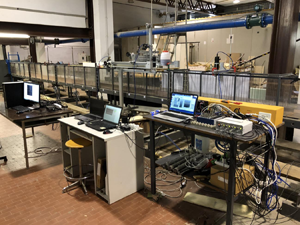
The experiments were carried out in a rectangular flume of the Hydraulic Laboratory at the Department of Civil, Environmental, Land, Building Engineering and Chemistry (DICATECh) of the Polytechnic University of Bari, Italy (figure 12). The channel is 25 m long, 0.40 m wide and 0.50 m high, and it is made of Plexiglas to guarantee optical access.

Figure 12. Experimental set-up at the Polytechnic University of Bari, where UPs are the ultrasonic probes.

The water recirculates through the channel in two partially separated circuits, each fed by a different tank. More precisely, the main circuit maintains steady flow conditions via a first constant head tank, whilst a secondary tank can discharge up to $0.080\,\textrm {m}^3\,\textrm {s}^{-1}$ by regulating a software-controlled electro-valve Bellino, thus generating a wave due to the flow rate change. A triangular sharp-crested weir in the downstream tank is used to estimate the steady flow rate, while a more accurate measure of the flow rate from the secondary tank is provided by an electromagnetic flowmeter placed upstream of the channel. The water level of the flume was $h=0.12\,\textrm {m}$ and was controlled by a sloping ($1\,:\,50$) gravel beach. Figure 13(a) shows a view of the flume section with the stem array, and figure 13(b) shows the electro-valve.

Figure 13. Some photos of the complex experimental apparatus: (a) a view of the flume; (b) the electro-valve.

A six-metre-long stem array was housed within the flume at 5.85 m from the channel inlet. The stem array consists of a set of rigid steel cylinders with diameter $d=3\,\textrm {mm}$, inserted into six previously drilled Plexiglas panels. Three different cylinder densities and patterns are obtained using the regular grid of holes longitudinally and transversely spaced with the same axis-to-axis distance (i.e. $s=4\,\textrm {cm}$). As shown in figure 14, the stem patterns for the three tested configurations are characterized by a density $n$ equal to (a) $156.25\, \textrm {cylinders}\,\textrm {m}^{-2}$, (b) $312.5\,\textrm {cylinders}\,\textrm {m}^{-2}$, and (c) $625\,\textrm {cylinders}\,\textrm {m}^{-2}$. Figure 15 shows a photo of the stem array, and table 2 shows the main parameters of the runs.

Figure 14. Obstacle patterns for the three tested configurations.

Figure 15. Side view of the stem array.

The free surface variation in the flume is measured by six ultrasonic probes at a 100 Hz sampling rate. The probes are located at $x=7.50$, 9.00 and 10.50 m, so that the three sensors measure wave attenuation along the stem array (see figure 12, which includes the $x,z$ reference coordinate system).

Table 2. Values of some parameters of the experimental runs of solitary waves.

A solitary-like wave was generated, reaching flow peak $0.085\,\textrm {m}^3\,\textrm {s}^{-1}$, as the sum of a steady flow $0.010\,\textrm {m}^3\,\textrm {s}^{-1}$ and an unsteady flow produced by linearly opening and closing the electro-valve for 10 s and 20 s, respectively.

Figure 16 shows a comparison between the wave height data measured and those obtained with the theoretical model. The comparison highlights the agreement between the aforementioned data even in the case of a solitary wave superimposed on a background current. The measured wave damping through vegetation is the combined result of vegetation and wall friction. Even though the combined effect is expected to be greater than the wave attenuation induced by vegetation alone, the order of magnitude of wave damping caused by an array of stems is significantly higher compared to wall friction. In this regard, the experiments were conducted in a vegetated section of the channel that was sufficiently long to achieve significant wave damping but short enough for wall effects to be entirely negligible. For this purpose, reference was also made to Huang et al. (Reference Huang, Yao, Sim and Yao2011).

Figure 16. Comparison between theoretical and experimental solitary wave heights: (a) test Exp1, (b) test Exp2, (c) test Exp3.

3.3. The bulk drag coefficient

Figure 17 shows the values of the bulk drag coefficients of waves analysed numerically and experimentally, and described in the previous subsections. The same figure also shows the trend of the drag bulk coefficients proposed by Nepf (Reference Nepf1999) as a function of array density $ad$, together with the range of variability of the experimental data indicated by the author. The wake interference model of Nepf (Reference Nepf1999) predicts that the bulk drag coefficient $C_D$ decreases with increasing $ad$ for random and staggered arrays. As highlighted in the original diagram by Nepf (Reference Nepf1999), the experimental data show a certain scatter with respect to the line shown in figure 17.

Figure 17. Diagram of the experimental values of the bulk drag coefficient $C_D$ with the fitting line and the variability range of the experimental data from the literature (Nepf Reference Nepf1999).

The results for the bulk drag coefficients obtained in this study are in good agreement with those reported by Nepf (Reference Nepf1999), even when considering the fact that the latter's data pertain to a steady flow condition. This conclusion holds both for the case of waves alone and for waves superimposed on a background current. The bulk drag coefficient of the experimental configurations tends to be smaller than those identified by the curve in figure 17, even though it is in the range of the error bars of that curve. As indicated in § 2.1, high sheltering, linked to a lower value of $s/d$, involves a reduction in the drag force, due to the fact that downstream cylinders can be placed in the wakes of upstream elements. Even if the dimensionless distances $s/d$ for the three experimental runs are greater than for the numerical configurations (see the comparison of the values of the parameter $s/d$ in tables 1 and 2), the presence of a background current in the experimental tests creates a certainly more effective wake, resulting in a smaller drag force. Nevertheless, in the case of solitary waves with a background current, the experimental data for $C_D$ confirm the trend known from the literature, whereby for values $ad<0.001$, the value of $C_D$ is, on average, constant.

Gijón Mancheño et al. (Reference Gijón Mancheño, Jansen, Uijttewaal, Reniers, van Rooijen, Suzuki, Etminan and Winterwerp2021) also showed a dependence of the bulk drag coefficient as a function of the Keulegan–Carpenter number (Keulegan & Carpenter Reference Keulegan and Carpenter1958), defined as the ratio between the drag and the inertia forces, given by the ratio between the horizontal excursion of the orbital movement of the water particles in the presence of wave motion and the diameter of the stems. The dependence of $C_D$ on the Keulegan–Carpenter number has also been highlighted by Wang, Yin & Liu (Reference Wang, Yin and Liu2022) for the case of gravity waves. As stated previously, it is worth noting that the drag coefficient values reported by Nepf (Reference Nepf1999) do not pertain to wave motion. Therefore, it is particularly interesting to compare the bulk drag coefficient data presented in this paper with those from Wang et al. (Reference Wang, Yin and Liu2022). In their study, Wang et al. (Reference Wang, Yin and Liu2022) conducted physical experiments using a 10-metre-long model representing a mature Rhizophora forest to investigate hydrodynamic characteristics and the attenuation of gravity waves. They introduced a novel parameter, i.e. a modified Keulegan–Carpenter number $KC_{r_v}=u_pT/r_v$, where $u_p=u(1-\phi )$ is the spatially averaged flow velocity in the spaces among the stems, with $u$ the flow velocity, $r_v=({{\rm \pi} }/{4})(({1-\phi })/{\phi })d$ a hydraulic radius related to obstacles, and $T$ the wave period. This parameter signifies the spatially averaged flow velocity within the interstices among the stems. Finally, the authors established a correlation between the bulk drag coefficient and $KC_{r_v}$, producing an empirical formula for $C_D$. The authors observed that this formula elucidates the drag coefficient attributes of obstacles with a notably high degree of correlation.

Although the waves in this study are solitary waves, thus different from those analysed by Wang et al. (Reference Wang, Yin and Liu2022), efforts were made to compare the values of the drag coefficients from numerical and experimental runs to assess the feasibility of extending the analysis of the authors. For the configurations in this study, the computation of $KC_{r_v}$ was performed as follows. The value of the wave period $T$ is based on the wavelength, calculated using (2.5), and the celerity of waves in shallow water, as proposed by Munk's theory of solitary waves (Munk Reference Munk1949). The velocity values $u$ at the passage of the soliton crest, which enabled us to compute $u_p=u(1-\phi )$, were obtained from the numerical SPH code for the numerical configurations and experimentally for laboratory tests. Specifically, the velocity scale $u$ for numerical configurations is approximately $O(1.5\,\textrm {m}\,\textrm {s}^{-1})$, while for experimental configurations it is approximately $O(1\,\textrm {m}\,\textrm {s}^{-1})$. Figure 18 illustrates that the $C_D$ values proposed in this study align very well, even with the theoretical framework proposed by Wang et al. (Reference Wang, Yin and Liu2022), whose fitted curve has the equation

(3.4)\begin{equation} C_{D}=\left ( \frac{0.77}{KC_{r_v}} \right)^{0.41} +0.42. \end{equation}

Figure 18. Relationship between $KC_{r_v}$ and the $C_D$ data of three vegetation models of Wang et al. (Reference Wang, Yin and Liu2022), with their theoretical curve, their proposal of a 95 % prediction band, and the data of the present study.

Therefore, it can be concluded that the present study allows for extending the trend of the bulk drag coefficient by Wang et al. (Reference Wang, Yin and Liu2022), both for solitary waves alone and for solitary waves with a background current, within the limits of the experiment performed. Furthermore, it is possible to conclude that the order of magnitude of $C_D$ is also in agreement with Nepf (Reference Nepf1999). This is because solitary waves fall within the category of long waves, i.e. flows that, although of a wave-induced type, are those that most closely resemble stationary currents.