


1 Introduction
The movement of fluids in porous media has been widely studied in various fields. A porous medium initially saturated with a fluid can undergo implosive collapse due to a change in pore pressure (Bueno & Gomez Reference Bueno and Gomez2016; Alvarez Reference Alvarez2017). An alteration in fluid properties at a large scale could lead to creep formation (Zhu, He & Yin Reference Zhu, He and Yin2014). In addition, polyaxial stresses acting on a porous medium in the presence of pore fluids can induce significant deformation. Such occurrences may significantly alter the hydromechanical equilibrium of the porous media, especially in samples with low-to-medium compressive strength. It has been shown that stress application has a controlling influence on pore-size distribution, porosity, tortuosity, absolute permeability, relative permeabilities and capillary pressure (Zhu & Wong Reference Zhu and Wong1996). Therefore, it is clear that the hydromechanical interactions between the fluids located in pore spaces and adjacent structures need to be accounted for. Models for interactions between fluids and solids should be coupled within a robust framework (Zienkiewicz, Taylor & Taylor Reference Zienkiewicz, Taylor and Taylor2000; Zhang & Tahmasebi Reference Zhang and Tahmasebi2018; Tahmasebi & Kamrava Reference Tahmasebi and Kamrava2019).
In the literature, the traditional approach for achieving fluid–solid coupling is referred to as fluid–structure interaction (FSI). A joint finite element methodology is typically used to solve equations for both fluids and solids, along with the deforming interface (Bathe, Zhang & Ji Reference Bathe, Zhang and Ji1999; Rugonyi & Bathe Reference Rugonyi and Bathe2001; Bathe & Zhang Reference Bathe and Zhang2004; Vierendeels et al. Reference Vierendeels, Lanoye, Degroote and Verdonck2007; Sathe & Tezduyar Reference Sathe and Tezduyar2008). Another technique that has gained significant recognition is the hybrid technique of employing finite volume (FV) for the fluid domain and finite element (FE) for the solid. This technique takes advantage of the strength of both solvers, given that FE is conventionally applied to solving computational solid mechanics equations while FV is used for computational fluid dynamics (known as CFD) problems (Campbell Reference Campbell2010; Munsch & Breuer Reference Munsch, Breuer, Bungartz, Mehl and Schäfer2010). Other techniques include lattice Boltzmann method finite element (known as LBM*-FE) (Kollmannsberger et al. Reference Kollmannsberger, Geller, Duster, Tolke, Sorger, Krafczyk and Rank2009; Geller et al. Reference Geller, Kollmannsberger, Bettah, Krafczyk, Scholz, Duster, Rank, Bungartz, Mehl and Schäfer2010) and discrete element method (known as LBM*-DEM) (Han & Cundall Reference Han and Cundall2012); the asterisk denotes flow solvers.
Coupled methods can be classified as either monolithic or partitioned. In the monolithic approach, the governing equations are solved within the same computational framework; in the partitioned approach, both equations are solved separately and then coupled via coupling algorithms. The latter is less memory intensive and easier to implement. However, some aspects such as code-to-code communication or grid-to-grid interpolation (e.g. of loads and displacements) must be considered. The monolithic approach, on the other hand, requires a multidisciplinary approach in which communication between both solvers occurs synchronously within the same code. The solutions tend to be more accurate than those generated by the partitioned approach; however, they can be very memory intensive, and it may be difficult to manage the codes. This paper, therefore, focuses only on the partitioned method.
Some of the difficulties encountered in coupled fluid–solid solver applications are that the partial differential equations are always nonlinear in nature, and analytical equations often do not exist to validate the results. Some data have been made available for numerical benchmarking of problems involving elastic deforming structures in the presence of laminar incompressible flow (Turek & Hron Reference Turek and Hron2006; Turek et al. Reference Turek, Hron, Razzaq, Wobker, Schäfer, Bungartz, Mehl and Schäfer2010), as well as experimental data (Gomes & Lienhart Reference Gomes, Lienhart, Bungartz and Schäfer2006). Nevertheless, the time-consuming nature of the simulations, especially for porous media applications (as shown in table 1), remains a major problem. For example, the physical/CPU time required to directly solve for two-phase flow alone, through a segmented  $120^{3}$ voxels sandstone rock geometry, of porosity 23 % and 502 k cells, is approximately nine hours or more depending on the application. For a coupled system of the same geometry, it takes nearly
  $5\times 9~\text{h}$, even with a supercomputer cluster of 200 cores. Consequently, in this study we attempt to improve computational efficiency by applying a meshless technique for the fluid while still maintaining a boundary-fitted technique for the solid, to ensure optimal accuracy for the coupled model.
Table 1. Comparison of the computational times for various coupled pore-scale solvers on a domain with  $120^{3}$ voxels. Note that the review of speeds of coupled solvers includes the preliminary results of this work. Similar step size and different cell sizes were used. Coupled and decoupled solutions were performed using multiphase fluids, while the stand-alone fluid simulations were performed for both multiphase (with FV) and single-phase flow (with FE). The central processing unit, CPU, time is reported in minutes. The FE-DPN*, which is the method implemented in this work, came out fastest by far in all categories; DPN represents dynamic pore network.

a Number of nodes and throats.
Note: The cells indicated for the DPN* are the number of pore bodies and throats divided by 1000.
Direct simulation methods for fluid solvers tend to be time-consuming, especially for multiphase fluid simulation (Joekar-Niasar & Hassanizadeh Reference Joekar-Niasar and Hassanizadeh2012). In general, the pore network (PN) method (Fatt Reference Fatt1956) is an efficient alternative for modelling pore-scale processes, using ideal geometries. The entire porous medium is represented as a network of nodes (pore bodies) and connecting channels (throats) comprising circular and triangular cross-sections, as well as other descriptive elements. This technique has been adopted for a wide range of applications, including two-phase flow (Bryant & Blunt Reference Bryant and Blunt1992; Blunt Reference Blunt1995; Oren, Bakke & Arntzen Reference Oren, Bakke and Arntzen1998), foam injection (Kharabaf & Yortsos Reference Kharabaf and Yortsos1998; Chen, Yortsos & Rossen Reference Chen, Yortsos and Rossen2005), drying processes (Figus et al. Reference Figus, Bray, Bories and Prat1999), contaminant transport (Bijeljic & Blunt Reference Bijeljic and Blunt2007) and three-phase flow (Pereira et al. Reference Pereira, Pinczewski, Chan, Paterson and Oren1996). Although PN far surpasses other flow solvers in terms of speed, its accuracy has often been questioned because it simplifies the pore-space geometry. This idealization could lead to loss of geometric and topological information. However, some models have been shown to yield an acceptable match with experimental values for relative permeability and capillary-saturation curves (Oren et al. Reference Oren, Bakke and Arntzen1998).
In this work, we develop a new segregated coupled pore-scale solver in which DPN (a variation of PN) is used for simulating multiphase fluid flow, while FE is used for solving the solid equations. The use of DPN can be a valuable tool in coupled pore-scale modelling, as it can be quite fast and can potentially be applied to larger domains. Here, DPN is used for modelling the fluid system based on prescribed inlet flow rate boundary conditions. The solid is assumed to experience large deformations; therefore, it is modelled as a nonlinear elastic material. A fictitious fluid–solid interface is created at the DPN-finite element node junction via convex hulling, followed by data exchange using linear interpolation.
The rest of this paper is arranged as follows: the first section examines the equations of the fluid and solid solvers, including the coupling methodology; the next section examines the application for an elastically deforming rock matrix experiencing drainage in a water-wet system. We then verify the model with respect to an FV model.
2 Methodology
We study the response of an elastic porous medium interacting with immiscible and incompressible fluids. We focus on three-dimensional geometries while considering large displacements of the rock matrix. The fluid motion is modelled using DPN and the solid deformation is modelled using the FE methodology. The fluid in the network interacts with the solid matrix, inducing elastic deformation; and this deformation leads to changes in pore pressure, thus giving rise to two-way hydromechanical coupling. We neglect the effect of gravitational forces in this work because of the scale of investigation. Both models are coupled using a segregated or partitioned approach and linked together via a fictitious boundary.
2.1 DPN flow model
In DPN, the spatial arrangements of pores and throats are obtained directly from segmented images. In this work, this was achieved using the maximal ball method (Dong & Blunt Reference Dong and Blunt2009), which can perform direct mapping of the actual sample to an irregular lattice. We calculated the pore body volumes and throat conductances based on the void space geometry. The pores are commonly represented in cubic or spherical form. For pore throats, however, a variety of geometric shapes with various cross-sections such as stars, circles, triangles, squares, etc., could be used. In this work, we use spherical pore bodies and cylindrical throats. Figures 1 and 2 show a typical arrangement of a network, with pore bodies (nodes) indicated by indices  $i$ and
  $j$, and throats
  $l_{ij}$ connecting both nodes
  $i$ and
  $j$. Depending on the driving mechanism, PN can be implemented either quasi-statically or dynamically. In quasi-static PN modelling, invasion of the pores is based solely on capillary entry pressure. Capillary pressure is imposed through boundary conditions on the network lattice. The position of fluid–fluid interfaces is then determined at each stage of the fluid displacement process independent of the time of the simulation, then the simulation runs until an equilibrium is attained between the prescribed capillary pressure and that of the system. If the interface is unstable, it moves through the network until a stable position is found or until it reaches the outlet. No time dependence is included in the calculation and the interface simply moves from one equilibrium position to another (Celia, Reeves & Ferrand Reference Celia, Reeves and Ferrand1995). Quasi-static models can be considered extensions of simple percolation models, with drainage floods being modelled through invasion percolation and imbibition through adapted bond percolation processes (Li, Mcdougall & Sorbie Reference Li, Mcdougall and Sorbie2017).

Figure 1. A local PN structure.

Figure 2. A subsample or elementary volume used for coupling simulations.
Quasi-static systems are not time dependent and are, consequently, unsuitable for the problem at hand due to the transient nature of the coupled system whose fluid and structural properties must evolve with time. Therefore, we employ a dynamic approach. In DPN systems, the model solves the pressure evolution problem based on capillary entry pressure and introduces a time dependent pore-filling mechanism. The emergent rate-dependent flow regimes are determined by a competition between capillary and viscous forces. The DPN model calculates the pressure forces by solving pressure evolution based on minimum filling time for each of the pores, which are eventually imparted onto the solid phase. If the pores are located in domain  $\unicode[STIX]{x1D6FA}_{f}$, and fluid flow in the pore throats is laminar, given Poiseuille’s law, each fluid phase obeys the following volume conservation law:
 $$\begin{eqnarray}V_{i}\frac{\unicode[STIX]{x2202}S_{i}}{\unicode[STIX]{x2202}t}+\mathop{\sum }_{i\in N}Q_{ij}=0,\quad \text{in }\unicode[STIX]{x1D6FA}_{f}\end{eqnarray}$$
 where  $N$ is the number of pore bodies,
  $V_{i}$ is the volume of pore body
  $i$,
$i$,  $S_{i}$ represents the local saturation of the reference phase and
  $Q_{ij}$ is the total volumetric flux from pore body
  $i$ to pore body
  $j$. If a channel or throat is completely filled with a single fluid, the flow rate along the throat from pore body
  $i$ to pore body
  $j$ can be calculated by
 $$\begin{eqnarray}Q_{ij}=G_{ij}(\unicode[STIX]{x1D6F7}_{i}-\unicode[STIX]{x1D6F7}_{j}),\end{eqnarray}$$
 where  $\unicode[STIX]{x1D6F7}_{k}$ is the hydraulic potential in pore body
  $k=\{i,j\}$ defined as
  $P_{k}+\unicode[STIX]{x1D70C}\boldsymbol{g}h_{k}$, where
  $h_{k}$ is the coordinate of the pore
  $k$ in the direction of the gravitational field,
  $P_{k}$ is the fluid pressure in pore
  $k$,
$k$,  $\boldsymbol{g}$ is the gravitational force and
  $G_{ij}$ is the throat conductance, defined as
 $$\begin{eqnarray}G_{ij}=\frac{S_{\unicode[STIX]{x1D6FC}}r_{ij}^{4}}{l_{ij}\unicode[STIX]{x1D702}},\end{eqnarray}$$
 where  $S_{\unicode[STIX]{x1D6FC}}$ is the shape factor,
  $r_{ij}$ is the radius of the connecting throat,
  $l_{ij}$ is the length of the throat taken from the centroids of pore body
  $i$ and pore body
  $j$, and
  $\unicode[STIX]{x1D702}$ is the fluid viscosity. The conductance is calculated at every throat location and is dependent on its radius and length. By applying a pressure gradient across the network (via boundary conditions), the pressure field inside the network can eventually be obtained by applying mass conservation at each interior node
  $i$,
$i$,
 $$\begin{eqnarray}\mathop{\sum }_{i\in N_{i}}Q_{ij}=0.\end{eqnarray}$$
For more than one fluid occupying the throat, the effects of capillary pressure must be accounted for across the fluid–fluid interface. The DPN model can be further simplified by using a circular throat cross-section, which prevents corner flow. For the case of drainage, if the displacement occurs in a piston-like manner and the effects of gravity are neglected, equation (2.2) is rewritten as
 $$\begin{eqnarray}Q_{ij}=G_{ij}(P_{i}-P_{j}-\unicode[STIX]{x0394}P_{ij}^{c}),\end{eqnarray}$$
where
 $$\begin{eqnarray}G_{ij}=S_{\unicode[STIX]{x1D6FC}}r_{ij}^{4}\left(\frac{1}{l_{ij}^{(i)}\unicode[STIX]{x1D702}_{i}}+\frac{1}{l_{ij}^{(j)}\unicode[STIX]{x1D702}_{j}}\right).\end{eqnarray}$$
 In equation (2.6),  $\unicode[STIX]{x1D702}_{i}$ and
  $\unicode[STIX]{x1D702}_{j}$ are the viscosities of the fluids in segments of the pore throats adjacent to pore
  $i$ and pore
  $j,$ while
  $l_{ij}^{(i)}$ and
  $l_{ij}^{(j)}$ are the corresponding segment lengths. The capillary pressure jump between the fluid–fluid interface is expressed by the Young–Laplace equation,
 $$\begin{eqnarray}\unicode[STIX]{x0394}P_{ij}^{c}=\unicode[STIX]{x1D6FE}_{sf}\cos \unicode[STIX]{x1D703}\left(\frac{1}{R_{1}}+\frac{1}{R_{2}}\right),\end{eqnarray}$$
 where  $R_{1}$ and
  $R_{2}$ are the radii of curvature of the interface in any two orthogonal planes,
  $\unicode[STIX]{x1D703}$ is the contact angle and
  $\unicode[STIX]{x1D6FE}_{sf}$ is the surface tension. For a given distribution of fluids, the phase conductances are calculated from (2.6). The pressure fields can be computed by substituting (2.5) into (2.4), which yields the following linear system of equations:
 $$\begin{eqnarray}[\unicode[STIX]{x1D642}]\{\boldsymbol{P}\}=[\boldsymbol{B}],\end{eqnarray}$$
 where  $\unicode[STIX]{x1D642}$ is the matrix of the conductivities,
  $\boldsymbol{P}$ is the vector of unknown nodal pressures and
  $\boldsymbol{B}$ is a vector formed from boundary pressures and capillary pressures. This equation can be solved using the biconjugate gradient solution method. The updated pressure field is then used in (2.5) to compute fluxes through the pore throats. Simulations can also be carried out with constant injection rate boundary conditions (Aker et al. Reference Aker, Jørgen Måløy, Hansen and Batrouni1998), which we used in this work. After solving for the volumetric fluxes of all capillary elements, the current invading phase saturation in each pore body is used to determine the minimum filling time for each of the pores; this is set as the time step size
  $\unicode[STIX]{x0394}t$. This time step corresponds to the shortest time required to fill one non-wetting phase-filled pore. Then, equation (2.1) is used to update the saturation in each pore body.
2.2 Finite element method
In this paper, the solid response is quantified using finite element formulation. We assume that the solid undergoes large deformations and, as such, we model the solid domain as nonlinear elastic. For a spatial solid domain  $\unicode[STIX]{x1D6FA}_{s}^{0}\subset \mathbb{R}^{d}$ bounded by
  $\unicode[STIX]{x1D6E4}$, the continuum equations can be described in total Lagrangian form as
 $$\begin{eqnarray}\displaystyle & \displaystyle \unicode[STIX]{x1D70C}_{0}\ddot{\boldsymbol{u}}=\unicode[STIX]{x1D735}_{0}\boldsymbol{\cdot }(\unicode[STIX]{x1D64E}\boldsymbol{\cdot }\boldsymbol{F}^{\text{T}})+\unicode[STIX]{x1D70C}_{0}\boldsymbol{b}\quad \text{in }\unicode[STIX]{x1D6FA}_{s}^{0}, & \displaystyle\end{eqnarray}$$
 $$\begin{eqnarray}\displaystyle & \displaystyle \boldsymbol{u}=\overline{\overline{\boldsymbol{u}}}\quad \text{on }\unicode[STIX]{x1D6E4}_{D}^{0}, & \displaystyle\end{eqnarray}$$
 $$\begin{eqnarray}\displaystyle & \displaystyle (\unicode[STIX]{x1D64E}\boldsymbol{\cdot }\boldsymbol{F}^{\text{T}})\boldsymbol{\cdot }\boldsymbol{n}=\overline{\overline{\boldsymbol{T}}}\quad \text{on }\unicode[STIX]{x1D6E4}_{N}^{0}, & \displaystyle\end{eqnarray}$$
 $0$ indicates the quantities related to the initial (undeformed) configuration, the displacement of the solid phase is denoted by
  $\boldsymbol{u}$, while each dotted accent represents the time derivative and
  $\boldsymbol{F}$ is the deformation gradient,
  $\boldsymbol{F}=\unicode[STIX]{x1D735}_{0}\boldsymbol{u}$. The Dirichlet and Neumann partitions at the boundaries are
  $\overset{}{\boldsymbol{u}}$ and
  $\overline{\overline{\boldsymbol{T}}}$, respectively. Here,
  $\boldsymbol{n}$ is the unit surface normal in the reference configuration,
  $\unicode[STIX]{x1D70C}_{0}$ is the initial density and
  $\boldsymbol{b}$ is the body force per unit mass. The stress is obtained in terms of the second Piola–Kirchoff stress tensor
  $\unicode[STIX]{x1D64E}$ and the Green strain tensor
  $\unicode[STIX]{x1D640}$. The first Piola–Kirchoff stress is related to
  $\unicode[STIX]{x1D64E}$ by
  $\unicode[STIX]{x1D64B}=\unicode[STIX]{x1D64E}\boldsymbol{\cdot }\boldsymbol{F}^{\text{T}}$. For a finite element discretization,
  $B_{oh}=\bigcup _{e=1}^{E}\unicode[STIX]{x1D6FA}_{s}^{e,\ast }$ which is a combination of
  $\unicode[STIX]{x1D6FA}_{0}^{e}$ and
  $\unicode[STIX]{x1D6E4}_{0}^{e}=\unicode[STIX]{x1D6E4}_{D}^{0}\cup \unicode[STIX]{x1D6E4}_{N}^{0}$. The finite-dimensional piecewise polynomial approximation
  $\boldsymbol{u}_{h}$,
  $\unicode[STIX]{x1D64B}_{h}$ of the solution is defined in the spaces
  $$\begin{eqnarray}\displaystyle & \displaystyle X_{h}^{k}=\{\boldsymbol{u}_{h}\in L^{2}(B_{oh})|[\boldsymbol{u}_{h}|_{\unicode[STIX]{x1D6FA}_{0}^{e}}\in \mathbb{M}^{k}(\unicode[STIX]{x1D6FA}_{0}^{e})\forall \unicode[STIX]{x1D6FA}_{0}^{e}\in B_{oh}]\}\subset X^{f}(B_{oh})=\mathop{\prod }_{e}(H^{1}(\unicode[STIX]{x1D6FA}_{0}^{e})),\qquad & \displaystyle\end{eqnarray}$$
 $$\begin{eqnarray}\displaystyle & \displaystyle S_{h}^{k}=\{\unicode[STIX]{x1D64B}_{h}\in [L^{2}(B_{oh})]^{2}|[\unicode[STIX]{x1D64B}_{h}|_{\unicode[STIX]{x1D6FA}_{0}^{e}}\in \mathbb{M}^{k}(\unicode[STIX]{x1D6FA}_{0}^{e})^{2}\forall \unicode[STIX]{x1D6FA}_{0}^{e}\in B_{oh}]\}\subset S^{f}(B_{oh})=\mathop{\prod }_{e}(H^{1}(\unicode[STIX]{x1D6FA}_{0}^{e}))^{2},\qquad & \displaystyle\end{eqnarray}$$
 where  $\mathbb{M}^{k}$ is the set of polynomial functions up to degree
  $k\geqslant 1$. Let
  $\unicode[STIX]{x1D6FF}\boldsymbol{u}_{h}$ be an arbitrary test function defined in the space
 $$\begin{eqnarray}\displaystyle X_{hc}^{k} & = & \displaystyle \{\!\unicode[STIX]{x1D6FF}\boldsymbol{u}_{h}\in X_{h}^{k}|[\!\unicode[STIX]{x1D6FF}\boldsymbol{u}_{h}=0\forall \boldsymbol{X}\in \unicode[STIX]{x2202}B_{oh},\forall t\in T\text{ and }\unicode[STIX]{x1D6FF}\boldsymbol{u}_{h}(t_{0})=0\forall \boldsymbol{X}\in B_{oh}\unicode[STIX]{x1D6FF}\boldsymbol{u}_{h}(t_{f})\nonumber\\ \displaystyle & & \displaystyle \qquad =0\forall \boldsymbol{X}\in B_{oh}\! ]\!\}.\end{eqnarray}$$
 The weak formulation of the expression is carried out by integration in the reference coordinate system by finding  $\boldsymbol{u}_{h}\in X_{h}^{k}$ and
  $\unicode[STIX]{x1D64B}_{h}\in S_{h}^{k}$, such that
 $$\begin{eqnarray}\displaystyle & & \displaystyle \mathop{\sum }_{e}\int _{\unicode[STIX]{x1D6FA}_{0}^{e}}(\unicode[STIX]{x1D70C}_{0}\ddot{\boldsymbol{u}}_{h}-\unicode[STIX]{x1D735}_{0}\boldsymbol{\cdot }\unicode[STIX]{x1D64B}_{h})\cdot \unicode[STIX]{x1D6FF}\boldsymbol{u}_{h}\,\text{d}V=\mathop{\sum }_{e}\int _{\unicode[STIX]{x2202}\unicode[STIX]{x1D6FA}_{0}^{e}}\overline{\overline{\boldsymbol{T}}}\boldsymbol{\cdot }\unicode[STIX]{x1D6FF}\boldsymbol{u}_{h}\,\text{d}S+\mathop{\sum }_{e}\int _{\unicode[STIX]{x1D6FA}_{0}^{e}}\unicode[STIX]{x1D70C}_{0}\boldsymbol{b}\boldsymbol{\cdot }\unicode[STIX]{x1D6FF}\boldsymbol{u}_{h}\,\text{d}V\forall \unicode[STIX]{x1D6FF}\boldsymbol{u}_{h}\nonumber\\ \displaystyle & & \displaystyle \qquad \in X_{hc}^{k},\forall t\in T.\end{eqnarray}$$
Based on the nonlinear dynamic behaviour of the solid, the following discrete nonlinear system of linear equations can be obtained:
 $$\begin{eqnarray}\unicode[STIX]{x1D648}\ddot{\boldsymbol{u}}(t)+\unicode[STIX]{x1D63E}\dot{\boldsymbol{u}}(t)+\boldsymbol{f}_{int}(t)=\boldsymbol{f}_{ext}(t),\end{eqnarray}$$
 where  $\unicode[STIX]{x1D648}$ is the
  $3N\times 3N$ mass matrix,
  $\unicode[STIX]{x1D63E}$ is the damping matrix,
  $\boldsymbol{f}_{int}(t)$ and
  $\boldsymbol{f}_{ext}(t)$ are the internal force vector and the external force vector from the fluid in
  $3N$ dimensions, respectively. Since the solution is solved using Lagrangian meshes,
  $\unicode[STIX]{x1D648}$ is time invariant. Vibration effects are not considered in this work, so the damping coefficient is zero. The mass matrix, internal and external forces follow as
 $$\begin{eqnarray}\displaystyle & \displaystyle \unicode[STIX]{x1D648}_{IJ}=\int _{\unicode[STIX]{x1D6FA}_{s}}\unicode[STIX]{x1D70C}_{0}N_{I}N_{J}\,\text{d}V, & \displaystyle\end{eqnarray}$$
 $$\begin{eqnarray}\displaystyle & \displaystyle (\boldsymbol{f}_{int,I})^{\text{T}}=\int _{\unicode[STIX]{x1D6FA}_{s}}\frac{\unicode[STIX]{x2202}N_{I}}{\unicode[STIX]{x2202}\boldsymbol{X}}\unicode[STIX]{x1D64E}\boldsymbol{\cdot }\boldsymbol{F}^{\text{T}}\,\text{d}V, & \displaystyle\end{eqnarray}$$
 $$\begin{eqnarray}\displaystyle & \displaystyle \boldsymbol{f}_{ext,I}=\int _{\unicode[STIX]{x1D6FA}_{s}}\unicode[STIX]{x1D70C}_{0}\boldsymbol{b}N_{I}\,\text{d}V+\int _{\unicode[STIX]{x1D6E4}_{N}^{0}}\overline{\overline{\boldsymbol{T}}}\boldsymbol{\cdot }N_{I}\,\text{d}S, & \displaystyle\end{eqnarray}$$
 where  $N_{I}$ is the shape function corresponding to node
  $I$. The internal and external nodal forces are functions of nodal displacement and time. The external loads are prescribed as a function of time incrementally. Therefore, assembling the fluid load requires the computation of the time-varying force exerted by the encompassing fluid on the solid across the interface.
2.2.1 Time discontinuous Galerkin method
To solve for the solid response, we apply the time-discontinuous Galerkin method (TDG) (Mancuso & Ubertini Reference Mancuso and Ubertini2003; Noels & Radovitzky Reference Noels and Radovitzky2008). A similar procedure has been used by De Rosis et al. (Reference De Rosis, Falcucci, Porfiri, Ubertini and Ubertini2014) for finite element method (FEM) coupling with the lattice Boltzmann method (LBM). However, their coupling methodology was applied only for linear dynamics. The TDG they applied can be easily adapted for nonlinear analysis, such as for Eulerian formulation (for example, see Denoël & Detournay (Reference Denoël and Detournay2011)). The TDG method considered in this work uses piecewise linear time interpolation. It is based on prediction and correction schemes, which can provide the requisite accuracy in a few iterations. The implementation is based on the Nørsett algorithm, which is optimal from the computational standpoint among higher-order unconditionally stable methods (Mancuso & Ubertini Reference Mancuso and Ubertini2002).
The integration is accomplished through the incremental solution procedure, in which the time interval of interest ( $T$) is discretized into
  $n^{f}$ time steps such that
  $T=\bigcup _{n=0}^{n=n^{f}-1}[t^{n},t^{n+1}]$ and
  $\unicode[STIX]{x0394}t=t^{n+1}-t^{n}$ is the time step. The scheme treats the displacement and velocity vectors as independent variables and uses piecewise linear time interpolants. The iterative scheme is summarized by the following equation:
 $$\begin{eqnarray}\displaystyle \left.\begin{array}{@{}c@{}}\displaystyle \unicode[STIX]{x1D648}^{\ast }\overline{\boldsymbol{v}}_{k}^{l+1}(t)=\boldsymbol{F}_{k}(t)-\frac{\unicode[STIX]{x2202}\boldsymbol{f}_{int}}{\unicode[STIX]{x2202}\boldsymbol{u}}\tilde{\boldsymbol{u}}_{k}^{l+1}(t),\\ \displaystyle \overline{\boldsymbol{u}}_{k}^{l+1}(t)=\tilde{\boldsymbol{v}}_{k}^{l+1}(t)+\unicode[STIX]{x1D707}\unicode[STIX]{x0394}t\overline{\boldsymbol{v}}_{k}^{l+1}(t),\end{array},\quad k=0,1;l=0,1\right\} & & \displaystyle\end{eqnarray}$$
 where  $\unicode[STIX]{x2202}\boldsymbol{f}_{int}/\unicode[STIX]{x2202}\boldsymbol{u}=\unicode[STIX]{x1D646}^{int}$ is the Jacobian matrix of the internal forces or the tangent stiffness matrix, and the barred terms represent time derivatives. The predictor displacements
  $\tilde{\boldsymbol{u}}_{k}$ and velocities
  $\tilde{\boldsymbol{v}}_{k}$ are given as
 $$\begin{eqnarray}\displaystyle & \displaystyle \tilde{\boldsymbol{v}}_{0}^{l+1}=\boldsymbol{v}_{\ast }^{t}+\unicode[STIX]{x1D706}^{\ast }\unicode[STIX]{x0394}t(\overline{\boldsymbol{v}}_{0}^{l}-\overline{\boldsymbol{v}}_{1}^{l}), & \displaystyle\end{eqnarray}$$
 $$\begin{eqnarray}\displaystyle & \displaystyle \tilde{\boldsymbol{u}}_{0}^{l+1}=\boldsymbol{u}_{\ast }^{t}+\unicode[STIX]{x1D706}^{\ast }\unicode[STIX]{x0394}t(\overline{\boldsymbol{u}}_{0}^{l}-\overline{\boldsymbol{u}}_{1}^{l})+\unicode[STIX]{x1D6FC}^{\ast }\unicode[STIX]{x0394}t\tilde{\boldsymbol{v}}_{0}^{l+1}, & \displaystyle\end{eqnarray}$$
 $$\begin{eqnarray}\displaystyle & \displaystyle \tilde{\boldsymbol{v}}_{1}^{l+1}=\boldsymbol{v}_{\ast }^{t}+(1-\unicode[STIX]{x1D6FC}^{\ast })\unicode[STIX]{x0394}t\overline{\boldsymbol{v}}_{0}^{l+1}, & \displaystyle\end{eqnarray}$$
 $$\begin{eqnarray}\displaystyle & \displaystyle \tilde{\boldsymbol{u}}_{1}^{l+1}=\boldsymbol{u}_{\ast }^{t}+(1-\unicode[STIX]{x1D6FC}^{\ast })\unicode[STIX]{x0394}t\overline{\boldsymbol{u}}_{0}^{l+1}+\unicode[STIX]{x1D6FC}^{\ast }\unicode[STIX]{x0394}t\tilde{\boldsymbol{v}}_{1}^{l+1}, & \displaystyle\end{eqnarray}$$
 $\boldsymbol{u}_{\ast }^{t}$ and
  $\boldsymbol{v}_{\ast }^{t}$ are the vector of unknown displacements and its time derivative at time
  $t$ of the FE solution. Here,
  $\unicode[STIX]{x1D648}^{\ast }$ is the effective mass matrix given by
  $$\begin{eqnarray}\unicode[STIX]{x1D648}^{\ast }=\unicode[STIX]{x1D648}+{\unicode[STIX]{x1D6FC}^{\ast }}^{2}\unicode[STIX]{x0394}t^{2}\frac{\unicode[STIX]{x2202}\boldsymbol{f}_{int}}{\unicode[STIX]{x2202}\boldsymbol{u}}.\end{eqnarray}$$
 It should be noted that this effective mass matrix is equally symmetric and positive-definite, just as  $\unicode[STIX]{x1D648}$ and
  $\unicode[STIX]{x1D646}^{int}$. The effective load
  $\boldsymbol{F}_{k}$ (in which the fluid loads would be transmitted) is obtained within two iterations. Based on the on left Radau abscissas, the effective loads are defined as
 $$\begin{eqnarray}\displaystyle & \displaystyle \boldsymbol{F}_{0}=\left(\frac{3\sqrt{2}}{4}-\frac{1}{2}\right)\boldsymbol{f}_{ext,0}+(6-3\sqrt{2})\boldsymbol{f}_{ext,2/3}, & \displaystyle\end{eqnarray}$$
 $$\begin{eqnarray}\displaystyle & \displaystyle \boldsymbol{F}_{1}={\textstyle \frac{3}{2}}\,\boldsymbol{f}_{ext,2/3}-{\textstyle \frac{1}{2}}\boldsymbol{f}_{ext,0}, & \displaystyle\end{eqnarray}$$
 where  $\boldsymbol{f}_{ext,0}$ is the value of
  $\boldsymbol{f}_{ext}$ at time
  $t$ and
  $\boldsymbol{f}_{ext,2/3}$ is the value at time
  $t+2/3\unicode[STIX]{x0394}t$. Coefficients
  $\unicode[STIX]{x1D706}^{\ast }$ and
  $\unicode[STIX]{x1D6FC}^{\ast }$ are given as follows:
 $$\begin{eqnarray}\unicode[STIX]{x1D706}^{\ast }=\sqrt{2}-\frac{4}{3},\quad \unicode[STIX]{x1D6FC}^{\ast }=1-\frac{\sqrt{2}}{2}.\end{eqnarray}$$
The model is iterated twice to achieve third-order accuracy. To complete the TDG algorithm, the following equations are solved at the end of the current time step:
 $$\begin{eqnarray}\boldsymbol{v}_{\ast }^{n+1}=\overline{\boldsymbol{u}}_{1}^{l},\quad \boldsymbol{u}_{\ast }^{n+1}=\boldsymbol{u}_{\ast }^{n}+\unicode[STIX]{x0394}t[(1-\unicode[STIX]{x1D6FC}^{\ast })\overline{\boldsymbol{u}}_{0}^{l}+\unicode[STIX]{x1D6FC}^{\ast }\overline{\boldsymbol{u}}_{1}^{l}].\end{eqnarray}$$
2.3 Coupled model
As stated previously, this work aims to develop a three-dimensional fluid–solid model incorporating FE and DPN. Both solution domains are illustrated in figure 3. Pore fluids exert forces on the solid walls, resulting in deformation and eventual modification of force balance. Additionally, the deformation of the solid results in the rearrangement of its structure which can alter fluid properties and the network topology. Thus, the need to update the network regularly during the simulation to track the deformation of the solid. To achieve the solution of such a system, the fluidic and structural computations are performed sequentially. Therefore, at each time step, we began by solving the DPN equation, from which we obtain the pressure at each node and throat. The DPN solver then feeds the hydrodynamic load to the solid at each time-exchange step. The FE solver computes the solid displacement  $\boldsymbol{u}$, which is then used to determine the new structure of the DPN.

Figure 3. Schematic of the superimposed domains (fluid and solid). (a) The voxelized solid phase along with the PN and (b) discretized finite element domain and PN.
More precisely, the updated set of displacements are used to compute the new position of the solid boundary. The structural computation updates the position of the structural surface. Thus, an updated fluid domain is needed to accommodate the new interface location. We achieved this by performing a re-extraction process for the network. This provides a new value for the node radius  $\{r_{i}^{\prime }\}$ and volume
  $\{V_{i}^{\prime }\}$, as well as a new throat length
  $\{l_{ij}^{\prime }\}$ and radius
  $\{r_{ij}^{\prime }\}$. An iterative process is also required at each time step to ensure that the coupled system converges to a steady solution before advancing to the next time step. This is done to reduce the magnitude of errors that could occur during the network re-extraction process. We examine this further in § 3. Another important aspect of the fluid–solid coupling procedure is the hydrodynamic load calculation. The force on the pore body is calculated with the following equation:
 $$\begin{eqnarray}\boldsymbol{F}_{i}=\int _{\unicode[STIX]{x1D6E4}_{i,f}}P_{i}\boldsymbol{n}\,\text{d}s,\quad \text{on }\unicode[STIX]{x1D6E4}_{i,f}\end{eqnarray}$$
 where  $\boldsymbol{F}_{i}$ is the pressure force applied by the
  $i$th pore with pore pressure
  $P_{i}$. The boundary of the
  $i$th pore is
  $\unicode[STIX]{x1D6E4}_{i,f}$ and
  $\boldsymbol{n}$ is the unit vector pointing from the centroid of the pore to the nearest solid boundary. Since we are using spherical DPN nodes, we assume the force is the same across the same pore-body node. The fluid load from the pore-body surface along the normal direction is imparted to the solid nodes. One of the central features in this coupling implementation is the exchange of information across the fluid and solid domains. As demonstrated in figure 3(a), the transmission of the fluid load to the solid would require a secondary domain for interfacing both subsystems since the adjoining pore bodies and solid do not match exactly.
2.3.1 Convex hull
In this work, the fluid loads are transmitted to solid nodal points that border an arbitrary volume surrounding the nearest pore body and throat. This initially requires test point values (spatial surface data) generated on the pore network, followed by a sequential neighbourhood search for FE nodal points within a prescribed region of the test point data. Several volumetric shapes could be used to enclose the points (e.g. the smallest cube or sphere). However, we use a convex hull, which is defined as the smallest convex set enclosing the points. The convex hull helps reduce the amount of empty space and saves memory. Calculation of convex hulls is a well-studied problem in computational geometry and this method has diverse applications in other fields, such as cluster analysis, collision detection, image processing, statistics, sphere packing and point location (Barber, Dobkin & Huhdanpaa Reference Barber, Dobkin and Huhdanpaa1996). It has also been applied in the natural element method (Sukumar, Moran & Belytschko Reference Sukumar, Moran and Belytschko1998), which relies on Delaunay triangulations in  $\mathbb{R}^{n}$, computed from convex hull in
  $\mathbb{R}^{n+1}$, to construct its interpolants. Convex hull has also been applied for modelling geophysical phenomena and complex FSI problems (Sukumar et al. Reference Sukumar, Moran and Belytschko1998). We define a convex hull as follows: for a set of randomly generated points
  $\unicode[STIX]{x1D6F6}^{k}=\{\unicode[STIX]{x1D6FE}_{\mathbf{1}},\unicode[STIX]{x1D6FE}_{\mathbf{2}},\ldots ,\unicode[STIX]{x1D6FE}_{\boldsymbol{N}}\}$ on the
  $k$th pore in
  $\mathbb{R}^{n}$, the convex hull
  $C$ of the points is expressed mathematically in the form
 $$\begin{eqnarray}C=\left\{\mathop{\sum }_{i=1}^{n}\unicode[STIX]{x1D706}_{i}\unicode[STIX]{x1D6FE}_{i}:\unicode[STIX]{x1D706}_{i}\geqslant 0\forall i\in \{1,\ldots ,n\}\wedge \mathop{\sum }_{i=1}^{n}\unicode[STIX]{x1D706}_{i}=1\right\}.\end{eqnarray}$$
 Equation (2.26) describes the convex combinations of points in set  $\unicode[STIX]{x1D6F6}$. For an
  $n$-dimensional convex hull set of nodal points, we apply the Quickhull (known as Qhull) algorithm developed by Barber et al. (Reference Barber, Dobkin and Huhdanpaa1996) to calculate the convex hull of sets of the multidimensional points of that hull. The hull is created based on random points (test points) generated on the surface of pores. Now for such a set of points, if a distinctive portion of the finite element nodal points (
 $\boldsymbol{n}=\{n_{1},n_{2},\ldots ,n_{M}\}$) and
  $\unicode[STIX]{x1D6F6}$ are found within the same space, they are labelled unity, while points outside are labelled zero. This process is graphically shown in figure 4. The forces
  $\boldsymbol{F}_{i}$ are then transmitted to nodes labelled unity while others outside this space, labelled zero, are left out.
Thus, at each time step, the coupling algorithm proposed in this work has the following sequence of operations:

3 Numerical results
The coupled technique was used to simulate the drainage of water by oil in a water-wet system in a Berea sandstone sample. The deformation of the solid was investigated during the drainage process. The DPN domain was extracted from the sandstone image such that the image in binary was defined by
 $$\begin{eqnarray}\displaystyle {\mathcal{I}}=\left\{\begin{array}{@{}l@{}}1,\quad Z\in \text{pore}\\ 0,\quad Z\in \text{solid},\end{array}\right. & & \displaystyle\end{eqnarray}$$
 where 1 represents the pores and 0 the solid. Here,  $Z$ denotes an arbitrary voxel in the binarized image. Extraction was achieved using the maximal ball algorithm (Dong & Blunt Reference Dong and Blunt2009). Tetrahedral meshes were generated directly from the image for the solid domain. The domain size (
 $L_{x}$,
  $L_{y}$,
  $L_{z}$) is (0.641, 0.641, 0.641) mm. Absolute permeability and void fraction are
  $210mD$ and 18.82 %, respectively. Details of the simulation parameters can be found in table 2.

Figure 4. Test points used for convex hulling. The hydrodynamic load is transferred to the solid mesh node points by linear interpolation of node points within the convex hull. Here,  $\unicode[STIX]{x1D716}_{i+r_{n}}$ represents the enlarged hull volume to include more points for interpolation. Points enclosed within
  $\unicode[STIX]{x1D716}_{i+r_{n}}$ are labelled as one. Points outside are zero.
Table 2. Properties used for the coupled simulation.

3.1 Boundary conditions
As mentioned earlier, DPN models are well suited for multiphase flow simulation. In this study, therefore, we considered a two-phase flow model, containing oil and water. We carried out drainage for a water-wet system (water is the wetting fluid and oil is the non-wetting fluid). Both fluids are incompressible and immiscible. The wetting phase has a dynamic viscosity of 1 cP and the non-wetting phase has a dynamic viscosity of 10 cP. Dynamic pore network simulation began with an injection of water across the network with a constant flow rate of  $1.25\times 10^{-13}~\text{m}^{3}~\text{s}^{-1}$ at the inlet. Simulation continued until after the length of the injection time was attained, which in this case was 20 s. The contact angle was set at
  $0^{\circ }$ at the inlet because only water was present at the start of the simulation and oil had not yet begun to displace water.
3.2 Results
At low flow rates, the capillary forces are more dominant than the viscous forces. This is governed by capillary number  $Ca=\boldsymbol{u}_{f}\unicode[STIX]{x1D707}/\unicode[STIX]{x1D6FE}_{sf}$, where
  $\boldsymbol{u}_{f}$ is the fluid velocity,
  $\unicode[STIX]{x1D707}$ is the dynamic viscosity and
  $\unicode[STIX]{x1D6FE}_{sf}$ is the interfacial tension. The viscous pressure drop (
 $\unicode[STIX]{x0394}P_{\unicode[STIX]{x1D707}}$) can play a major role when the flow rate is high when the characteristic length
  $L_{x}$ of the representative element volume is large, or in near-miscible displacements with low interfacial tension. Capillary pressure scales as
  $P_{c}=2\unicode[STIX]{x1D6FE}_{sf}/r_{c}\sim \unicode[STIX]{x1D6FE}_{sf}\sqrt{P_{\unicode[STIX]{x1D707}}/K}$, where
  $r_{c}$ is the mean radius of interfacial curvature. The viscous pressure drop scales as
  $\unicode[STIX]{x0394}P_{\unicode[STIX]{x1D707}}=\boldsymbol{q}_{f}\unicode[STIX]{x1D707}L_{x}/K$, where
  $K$ is the effective rock permeability. Therefore, the capillary pressure is not related to flow rate or
  $L_{x}$. When the ratio of viscous pressure drop to capillary pressure is high, macroscopic flow properties (e.g. relative permeability) can be a function of flow rate, leading to a Darcy law scenario in which flow rate nonlinearly depends on the pressure gradient. For this work, however, we only consider low flow rates that correspond to a capillary-dominated flow regime.
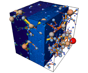
Figure 5 illustrates the drainage sequence at DPN simulation times. It can be observed that water sweeps the oil phase continually from the pore space by a piston-like displacement. Over time, more residing fluid was swept through the outlet. As the wetting phase was being displaced, we kept track of the hydrodynamic or pressure forces that are to be exchanged across the fictitious fluid–solid interface.

Figure 5. Drainage evolution in time for a water-wet system (oil is blue and water is red).
The deformation of the solid induced by fluid pressure is observed in figures 6 and 7. It can be seen that the forces at the throats are very small compared to those at the pores; thus, the forces at the throats can be ignored.

Figure 6. Solid deformed as a result of fluids residing in the pores at different pore pressures.
At the final time of the simulation, in figure 7(d), there is a greater distribution of pores with higher pressure forces than those in the earlier drainage sequence, because most of the pores have been invaded by the non-wetting phase. The deformation resulting from the local displacement of the wetting phase fluid is illustrated in figure 7(e–h), for which the maximum  $(5.67\times 10^{-5}~\unicode[STIX]{x03BC}\text{m})$ occurs at the end of the injection process.

Figure 7. Hydrodynamic forces and the corresponding deformation induced by nodal pressure in the network at times 1 s, 3 s, 5 s and 15 s, respectively.
We applied several random distributions to select the test points on the pore surface. Each test point was selected randomly from the interval  $[-r_{i,j},r_{i,j}]$. In this work, we considered data from 100 to 1000 random test points on each spherical pore body surface. We then conducted a sensitivity analysis for the optimum number of test points to be used for the simulations. Figure 8, for example, shows how the capillary pressure solution is affected by varying the number of test points. It can be observed in the earlier part of the displacement process (from the right-hand side) that the capillary pressure (
 $P_{c}$) values are more sensitive to the number of test points used; using more points lowers
  $P_{c}$ values by approximately 13.5 kPa. As water saturation decreases, this value becomes less dependent on the number of test points. Based on our preliminary results, 800 test points proved to be sufficient for our simulation. Another important parameter we considered in the coupling procedure is the tolerance/range of inclusivity. The apparent gap between both domains requires that the hull of pore body spatial points be enlarged to accommodate more FE nodal points, as seen in figure 4. This is achieved by defining a tolerance that can be interpreted as the range of FE points, away from the convex hull, which could still be regarded as an interpolation point. The tolerance and range of inclusivity are given as
 $$\begin{eqnarray}\unicode[STIX]{x1D716}_{i}=\unicode[STIX]{x1D702}\frac{\mathop{\sum }_{i}\unicode[STIX]{x1D6FE}_{i}}{N},\quad \unicode[STIX]{x1D716}_{i+r_{n}}=r_{n}+\unicode[STIX]{x1D702}\frac{\mathop{\sum }_{i}\unicode[STIX]{x1D6FE}_{i}}{N},\end{eqnarray}$$
 where  $\unicode[STIX]{x1D716}_{i}$ and
  $\unicode[STIX]{x1D716}_{i+r_{n}}$ are ranges of inclusivity,
  $\unicode[STIX]{x1D702}$ is a constant that depends on the size of the pore body radius
  $r_{\boldsymbol{i}}$ and
  $N$ is the total number of test points used for each pore body. Here,
  $r_{n}$ is a value that varies with
  $r_{i}$ where
  $r_{n}<r_{i}$. For all simulations, we examined the sensitivity of each FE node point
  $n_{k}$, with respect to
  $\Vert \unicode[STIX]{x1D716}_{i+r_{n}}\Vert$.

Figure 8. Effects of the number of test points on the capillary pressure solution for drainage in the water-wet system.
We also examined the effect of inflow volumetric rate on deformation in a four-case scenario while maintaining pre-existing boundary conditions. The first case, case A, had a flow rate of  $1.25\times 10^{-13}~\text{m}^{3}~\text{s}^{-1}$, while the base case (case B) had a flow rate of
  $2.5\times 10^{-13}~\text{m}^{3}~\text{s}^{-1}$. The flow rates of cases C and D were
  $5.0\times 10^{-11}~\text{m}^{3}~\text{s}^{-1}$ and
  $5.0\times 10^{-10}~\text{m}^{3}~\text{s}^{-1}$, respectively. Flow rates were increased and the subsequent deformation and von Mises stress were computed. The results are shown in figures 9(a) and 9(b), respectively. The deformation and stress increased monotonically for the flow rate up to a critical point, slightly below
  $1.0\times 10^{-10}~\text{m}^{3}~\text{s}^{-1}$. Thereafter, the solid deformed more significantly for all cases.

Figure 9. Evolution of (a) solid deformation and (b) the von Mises stress at different flow rates.

Figure 10. Convergence of pore network extractions.
A precoupling step was required, as indicated in algorithm 1, to ensure that the coupled system would converge to a steady solution before advancing to the next time step. The number of iterations would depend on the nature of the imaged data. The coordination number, which is the average number of pore bodies connected to a specific pore, could be affected based on the nature of the image from which the network is derived. Consequently, the stochastic nature of the maximal ball algorithm would generate inconsistent values for the maximum and minimum pore body and throat sizes for each re-extraction. Hence, we define a function  $E_{a}(\overline{X}_{p})$ which quantifies the error between each subiteration before the start of the transient coupling procedure. Each iteration
  $p$ signifies
  $p$ number of re-extractions performed. This error is defined by the following equation:
 $$\begin{eqnarray}E_{a}(\overline{X}_{p})=\frac{|\overline{X}(p)-\overline{X}(p+1)|}{\overline{X}(p)},\end{eqnarray}$$
 where  $\overline{X}(p)$ is the average value of the pore size at iteration
  $p$. This error allows us to estimate the accuracy of the extraction code, especially when boundary conditions are applied to the solid. In all of the proposed computational tests, the coupled system advances if
  $E_{a}(\overline{X}_{p})$ is smaller than a prescribed tolerance value. From figure 10, it is observed that the network extraction converged after four iterations.
3.3 The effect of boundary conditions during drainage
Several boundary loads were applied on the solid in the axial direction to investigate how such prescribed values affect flow properties. The absolute permeability and pore-size distribution were tracked as the simulation progressed. Figure 12(a) indicates the boundary conditions applied in this work. By applying a constant strain rate  $\dot{\unicode[STIX]{x1D73A}}(=\unicode[STIX]{x0394}z/(L_{z}\unicode[STIX]{x0394}t))$ at boundary
  ${\mathcal{B}}(x_{2})=L$, we monitored the deformation. A fixed constraint (zero displacement boundary condition) at boundary
  ${\mathcal{B}}(x_{2})=0$ was applied at the opposite boundary; rollers were used at the other boundaries to prevent the collapse of the solid normal to that boundary. The solid boundary loads were only applied at the beginning of the simulation, while the hydrodynamic forces were coupled at each subsequent iteration.

Figure 11. Solid deformation resulting from strain rates applied. Results are shown for two FE nodes, with 800 test points and  $\unicode[STIX]{x1D750}_{\boldsymbol{i}+\boldsymbol{r}_{\boldsymbol{n}}}=8\times 10^{-5}$.

Figure 12. (a) Solid boundary conditions used in microscale tests. (b) Pore pressure change.
Plots of solid displacement during loading are represented in figure 11. These results are taken at the same time corresponding to vertical strains of 0.00056 and 0.00160. The pore-size distribution (PSD) evolution is shown in figure 13 at different coupling times ranging from 1 s to 20 s. At these times, the results illustrate a shift in the PSD to the left, indicating a reduction in pore-size and the closures of some pores. There is also a vertical shift upwards, implying an increase in the number of smaller-sized pores. However, at much higher strain rate values, the distribution shifts downwards and the rest of the pore sizes are spread primarily to the right (with some to the left), indicating constriction as well as lateral dilation of some pores due to stress. The network also becomes distorted at equilibrium points as higher strain rate values are applied. Figure 14 shows a snapshot of the physical structure of the network after the deformation. The pore pressure also increases as the strain increases, as seen in figure 12(b). Another important property that we monitored during the deformation process was absolute permeability. Figure 15 shows the effect of the loading on absolute permeability. It can be observed that absolute permeability decreased as more load was applied. Furthermore, due to rearrangements of the pore network, precoupling iterations were carried out as shown in figure 10. It is apparent that the solution converged after four iterations.

Figure 13. Change in PSD with a load increase at fluid injection times 1 s, 4 s, 5 s, 8 s, 10 s and 14 s. There is an apparent shift to the left of the original plot when the solid is compacted in the axial direction, indicating a reduction in the pore radii. At a strain value of 0.01247, there is constriction as well as lateral dilation of some pores due to stress.

Figure 14. The network (a) before deformation and (b) after deformation. The differences between (a) and (b) are noted by white colouring in (b).

Figure 15. Absolute permeability evolution at different times.
3.4 Verification of results
We tested the results of the coupled FE-DPN* pore-scale model for accuracy. A coupled finite volume system was used as the basis for the comparison (Fagbemi, Tahmasebi & Piri Reference Fagbemi, Tahmasebi and Piri2020). The system constitutes a strongly coupled partitioned solver whose meshes are unstructured, independent and conformed at the interface. The hydrodynamic load is transmitted via face interpolation while the displacement is exchanged using vertex interpolation. The initial computational domain is an undeformed porous medium of size  $10^{3}~\text{mm}$. The sample geometry, and the preprocessing steps, are shown in figure 16. The drainage sequence began with the wetting phase occupying the entire computational fluid domain. Then, based on prescribed initial secondary fluid saturation, the non-wetting phase displaces the wetting phase.

Figure 16. The FV geometry, similar to the coupled model used in this work, was obtained using micro-CT imaging technology. To effectively study the effects of external stresses and fluid forces on the sample at the pore-scale, high-porosity Berea sandstone was used. The Berea image was initially filtered to improve the signal-to-noise ratio and then subsequently segmented into binary data, where each domain is represented by 0 or 1. The rock image sample has a pore volume fraction of 21.174 %. The original voxel size of the sample was  $1000^{3}$, which was later resized to
  $120^{3}$ for the simulation.
Similar flow rates were used, while a fixed pressure value boundary condition of zero was used at the outlet. No-slip boundary conditions were applied at the walls. Plots of deformation at selected mesh nodes, at the third time step from the last time  $\Vert d_{T-3}\Vert$, are compared for both solvers. As illustrated in figure 17, the results are in good agreement with those from the FE-DPN* model. The deformations for both solvers induced by fluid injection at lower flow rates are very similar. However, at higher flow rates, we begin to see a separation of values.

Figure 17. Verification of results for solid deformation from the finite volume model (FVM) and this work for selected nodal points, at the third time step from the last time  $\Vert d_{T-3}\Vert$.
4 Conclusion
We presented a new multimethod approach for studying fluid and solid interaction problems at the pore-scale. This approach drastically reduces the time required for computing results of the coupled solid and fluid analysis. We represented the pore structure as a network of spheres and cylinders for each pore and throat in space, respectively. The solid was represented using real segmented images generated by X-ray micro computed tomography (micro-CT) technology. The computational domain comprised a segregated two-way coupled system composed of a solid subdomain, having unstructured meshes whose nonlinear response was investigated using FEM; and a fluid subdomain whose flow characteristics was modelled using dynamic pore network method. Due to the meshless nature of the DPN and incongruity of the solid surface, hydrodynamic load transmission to the FE solver is a non-trivial task. In this work, continuity of stress was achieved by interpolation of fluid forces directly across a fictitious boundary. Solid nodal points and selected tested points on the surface of the pore bodies were interpolated within a convex hull of points based on a defined range of inclusivity. The deformation of the solid, which results in a rearrangement of its structure, required that the pore network be updated regularly during the simulation to track the deformation of the solid. The pore network was hence re-extracted at each time interval. Curtailing the host of potential errors from such a stochastic process required the implementation of several coupling subiterations which ensured that the average pore-size distribution was uniform at every time step. From our results, these errors were very minimal, indicating the potential of this technique for studying more complex interactions of fluid in complex solid media. We applied the coupled model for investigating solid deformation during the drainage process for capillary-dominated flow regimes. The effect of boundary conditions prescribed in the solid subdomain on the pore size distribution and absolute permeability were equally studied. Results from such computational experiments were then compared with those from a coupled finite volume solver, showing good agreement. One of the main applications of this approach is for modelling of deformation in large-scale problems for which direct numerical simulations and lattice Boltzmann methods for coupled systems are computationally expensive.
Acknowledgements
We would like to thank the University of Wyoming for financial support for this research. This study was partially supported by NSF (grant #CMMI-2000966), NIH (grant #P20GM103432) and NASA (grant #80NSSC19M0061).
Declaration of interests
The authors report no conflict of interest.


