


1 Introduction
Microstructured optical fibres (MOFs) are long and thin glass fibres that are typically approximately
 $150~\unicode[STIX]{x03BC}\text{m}$
in diameter and more than a kilometre in length. They contain a pattern of cylindrical air holes that run parallel to the axis of the fibre. To obtain a desired set of optical properties, the holes are required to have specific shapes and to be arranged in a particular pattern. This paper is concerned with the fluid mechanics of the fabrication of such fibres.
$150~\unicode[STIX]{x03BC}\text{m}$
in diameter and more than a kilometre in length. They contain a pattern of cylindrical air holes that run parallel to the axis of the fibre. To obtain a desired set of optical properties, the holes are required to have specific shapes and to be arranged in a particular pattern. This paper is concerned with the fluid mechanics of the fabrication of such fibres.
Fibres are drawn from a preform that is typically 1–3 cm in diameter and 10–20 cm in length. One of the major challenges in drawing MOFs is to determine the pattern of air holes that must be in the preform in order to achieve the desired hole pattern in the stretched fibre. The process is further complicated by the fact that significant amounts of heat are required during the drawing process to allow extension with moderate stretching forces. These thermal variations give rise to enormous variations in the viscosity of the glass during the drawing process. Thermal variations also give rise to variations in the surface-tension coefficient that are less dramatic than the variations in viscosity, but can nevertheless be significant. We will therefore develop a coupled flow and temperature model that describes the evolution of the shapes of the holes and the external boundary during the drawing process for fluids with temperature-dependent viscosity and surface tension. Despite the apparent complexity of the problem, we will show that the evolution can be obtained using a straightforward solution procedure.
The drawing of viscous threads has an extensive history with the pioneering work dating back to Matovich & Pearson (Reference Matovich and Pearson1969). Much of the early work considered solid threads (with no holes) in an isothermal setting and a review of the early work can be found in Denn (Reference Denn1980). For axisymmetric threads in an isothermal setting, a huge amount of work has been done in recent years. Kaye (Reference Kaye1991) devised a methodology to solve time-dependent extensional problems. A systematic derivation for extensional flows was undertaken by Dewynne, Ockendon & Wilmott (Reference Dewynne, Ockendon and Wilmott1992) and the analysis was generalised to include the effects of inertia and surface tension by Dewynne, Howell & Wilmott (Reference Dewynne, Howell and Wilmott1994). Yarin, Gospodinov & Roussinov (Reference Yarin, Gospodinov and Roussinov1994) developed a theory for the drawing of axisymmetric hollow tubes. Stokes et al. (Reference Stokes, Tuck and Schwartz2000) solved the problem of an inertialess solid thread falling under its own weight, inertial effects were included by Stokes & Tuck (Reference Stokes and Tuck2004), a very accurate numerical method was developed by Bradshaw-Hajek, Stokes & Tuck (Reference Bradshaw-Hajek, Stokes and Tuck2007) and the effects of surface tension were included by Stokes, Bradshaw-Hajek & Tuck (Reference Stokes, Bradshaw-Hajek and Tuck2011). Asymptotic solutions in the case with inertia were obtained for a thread extended by pulling with a fixed force at its ends by Wylie, Huang & Miura (Reference Wylie, Huang and Miura2011), for a thread falling under gravity by Wylie, Huang & Miura (Reference Wylie, Huang and Miura2015) and for a thread whose ends are pulled with a prescribed speed by Wylie, Bradshaw-Hajek & Stokes (Reference Wylie, Bradshaw-Hajek and Stokes2016). All of the above studies neglect thermal effects and are for axisymmetric threads, and therefore cannot be applied to MOFs that are subject to significant heating and have multiple holes.
Thermal effects for axisymmetric threads were first considered by Shah & Pearson (Reference Shah and Pearson1972a ,Reference Shah and Pearson b ) who examined how axial temperature variation affects stability of drawing. Further results for non-isothermal drawing were developed by Yarin (Reference Yarin1986) who considered how cooling affects unsteady extension. Gupta & Schultz (Reference Gupta and Schultz1998) developed asymptotic corrections to the one-dimensional models that arise in the long and slender asymptotic limit. Forest & Zhou (Reference Forest and Zhou2001) considered the sensitivity of drawing to transient fluctuations in the boundary conditions. Fitt et al. (Reference Fitt, Furusawa, Monro, Please and Richardson2002) developed a theory for heated axisymmetric tubes and carefully considered various asymptotic limits. Wylie & Huang (Reference Wylie and Huang2007) included the effects of viscous heating in unsteady extensional flows. Wylie, Huang & Miura (Reference Wylie, Huang and Miura2007) showed that non-uniqueness can occur if sufficiently large viscosity variations occur during the drawing process. Suman & Kumar (Reference Suman and Kumar2009) examined how draw ratio enhancement is affected by heating. Taroni et al. (Reference Taroni, Breward, Cummings and Griffiths2013) considered the relative importance of radiation, convection and conduction in the heating and cooling phases of glass drawing. He et al. (Reference He, Wylie, Huang and Miura2016) considered the evolution of a solid thread composed of a material whose viscosity and surface tension depend on temperature. All of these studies focussed on axisymmetric threads and so cannot be applied directly to MOFs that have multiple holes.
A number of authors have considered the non-axisymmetric case. Cummings & Howell (Reference Cummings and Howell1999) considered isothermal drawing for a solid thread with arbitrary shape and developed a novel transformation and Lagrangian solution procedure to determine the evolution of the shape of the thread. Griffiths & Howell (Reference Griffiths and Howell2007, Reference Griffiths and Howell2008) used similar techniques for a non-axisymmetric thread with a single hole and considered the limit of slender thin-walled tubes. Remarkably, they obtained an explicit solution for the shape of a thread with arbitrary initial cross-section. The problem of multiple holes was also studied by Stokes et al. (Reference Stokes, Buchak, Crowdy and Ebendorff-Heidepriem2014). They considered the case in which the surface tension coefficient does not depend on temperature and showed that, if one can tune the pulling tension to a required value (for example, by varying the heater temperature), then, surprisingly, one can obtain the shapes of the holes at the exit of a draw tower without any detailed knowledge of the temperature or viscosity profile in the device. This work was extended to include the effects of active channel pressurisation by Chen et al. (Reference Chen, Stokes, Buchak, Crowdy and Ebendorff-Heidepriem2015). Buchak et al. (Reference Buchak, Crowdy, Stokes and Ebendorff-Heidepriem2015) developed a technique to regularise the inverse problem and gravitational extension and extrusional flows were considered by Tronnolone et al. (Reference Tronnolone, Stokes, Foo and Ebendorff-Heidepriem2016) and Tronnolone, Stokes & Ebendorff-Heidepriem (Reference Tronnolone, Stokes and Ebendorff-Heidepriem2017).
However, for threads fabricated from fragile materials, measuring the fibre tension is problematic and hence the procedure of obtaining the shapes of the holes at the exit without any detailed knowledge of the temperature (Stokes et al. Reference Stokes, Buchak, Crowdy and Ebendorff-Heidepriem2014) cannot be applied. In addition, if the surface-tension coefficient depends on the temperature, the procedure also cannot be applied. So, in either of these cases, one must explicitly solve the thermal problem. One must also solve the thermal problem if one requires detailed information about the geometry of the thread in the draw tower rather than just the shape at the exit. For these reasons, we develop a fully coupled flow and temperature model that can describe the evolution of the thread and the holes throughout the drawing process. We show that, under a suitable transformation, the transverse motion of the thread decouples from the axial flow. The transverse flow can therefore be solved using standard techniques for Stokes flow problems in the absence of axial stretching. Having obtained the solution of the transverse-flow problem, one can then simply solve a system of three ordinary differential equations that completely determine the flow.

Figure 1. Schematic diagram of the neck-down region
 $0\leqslant x\leqslant L$
.
$0\leqslant x\leqslant L$
.
2 Model formulation
2.1 Full three-dimensional model
We consider a drawing device that feeds a thread of a viscous fluid (e.g. silica glass) with temperature
 $\unicode[STIX]{x1D703}_{in}$
through an aperture with a constant speed
$\unicode[STIX]{x1D703}_{in}$
through an aperture with a constant speed
 $U_{in}$
. We denote the square root of the cross-sectional area of the fluid as it comes through the aperture as
$U_{in}$
. We denote the square root of the cross-sectional area of the fluid as it comes through the aperture as
 $\unicode[STIX]{x1D712}_{in}$
. At a distance
$\unicode[STIX]{x1D712}_{in}$
. At a distance
 $L$
from the aperture, the thread is pulled by a take-up roller such that the thread has a speed
$L$
from the aperture, the thread is pulled by a take-up roller such that the thread has a speed
 $U_{out}$
. When it passes through the aperture, the thread has a pattern of
$U_{out}$
. When it passes through the aperture, the thread has a pattern of
 $N$
internal air channels (see figure 1). Between the aperture and a distance
$N$
internal air channels (see figure 1). Between the aperture and a distance
 $L_{h}<L$
, the thread is exposed to a radiative heater. Between the end of the heater and the take-up roller, the thread experiences radiative heat loss to the environment. Throughout the entire length of the thread, convective cooling also occurs as a result of a forced flow of cold gas through the device around the deforming thread.
$L_{h}<L$
, the thread is exposed to a radiative heater. Between the end of the heater and the take-up roller, the thread experiences radiative heat loss to the environment. Throughout the entire length of the thread, convective cooling also occurs as a result of a forced flow of cold gas through the device around the deforming thread.
MOFs are typically composed of glass or polymeric materials and these both have the property that their density, specific heat and conductivity do not change significantly with temperature. We therefore assume that they are all constant. On the other hand, the viscosity of these materials changes dramatically with temperature. Variations of the surface-tension coefficient with temperature are typically not as significant as variations in viscosity, but can nevertheless be significant (He et al. Reference He, Wylie, Huang and Miura2016).
We define a coordinate system with the
 $x$
-axis directed along the axis of the thread. We take
$x$
-axis directed along the axis of the thread. We take
 $x=0$
to be the location of the aperture and
$x=0$
to be the location of the aperture and
 $y$
and
$y$
and
 $z$
to be the coordinates in the cross-sectional plane. We denote the velocity vector, pressure and temperature by
$z$
to be the coordinates in the cross-sectional plane. We denote the velocity vector, pressure and temperature by
 $\boldsymbol{u}=(u,v,w)$
,
$\boldsymbol{u}=(u,v,w)$
,
 $p$
and
$p$
and
 $\unicode[STIX]{x1D703}$
, respectively. All of these dependent variables are, in general, functions of position
$\unicode[STIX]{x1D703}$
, respectively. All of these dependent variables are, in general, functions of position
 $\boldsymbol{x}=(x,y,z)$
and the time that we denote as
$\boldsymbol{x}=(x,y,z)$
and the time that we denote as
 $t$
. We denote the shape of the external boundary of the thread by
$t$
. We denote the shape of the external boundary of the thread by
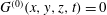 $G^{(0)}(x,y,z,t)=0$
and the shape of each of the
$G^{(0)}(x,y,z,t)=0$
and the shape of each of the
 $N$
internal holes to be
$N$
internal holes to be
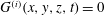 $G^{(i)}(x,y,z,t)=0$
,
$G^{(i)}(x,y,z,t)=0$
,
 $i=1,2,\ldots ,N$
. The outward pointing normal vectors on the boundaries are, hence, denoted by
$i=1,2,\ldots ,N$
. The outward pointing normal vectors on the boundaries are, hence, denoted by
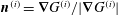 $\boldsymbol{n}^{(i)}=\unicode[STIX]{x1D735}G^{(i)}/|\unicode[STIX]{x1D735}G^{(i)}|$
. For convenience, we also define
$\boldsymbol{n}^{(i)}=\unicode[STIX]{x1D735}G^{(i)}/|\unicode[STIX]{x1D735}G^{(i)}|$
. For convenience, we also define
 $\unicode[STIX]{x1D712}^{2}(x,t)$
and
$\unicode[STIX]{x1D712}^{2}(x,t)$
and
 $\unicode[STIX]{x1D6E4}(x,t)$
to be the area of the cross-section and its total boundary length at axial position
$\unicode[STIX]{x1D6E4}(x,t)$
to be the area of the cross-section and its total boundary length at axial position
 $x$
. When the fluid passes through the aperture the velocity is
$x$
. When the fluid passes through the aperture the velocity is
 $u=U_{in}$
,
$u=U_{in}$
,
 $v=w=0$
, and we denote the area and the boundary lengths as
$v=w=0$
, and we denote the area and the boundary lengths as
 $\unicode[STIX]{x1D712}_{in}$
and
$\unicode[STIX]{x1D712}_{in}$
and
 $\unicode[STIX]{x1D6E4}_{in}$
, respectively. At the aperture, the shapes of the external boundary and the internal holes are denoted by
$\unicode[STIX]{x1D6E4}_{in}$
, respectively. At the aperture, the shapes of the external boundary and the internal holes are denoted by
 $G_{in}^{(0)}(y,z)=0$
and
$G_{in}^{(0)}(y,z)=0$
and
 $G_{in}^{(i)}(y,z)=0$
, respectively.
$G_{in}^{(i)}(y,z)=0$
, respectively.
Assuming an incompressible Newtonian fluid, the governing equations for the fluid flow are
 $$\begin{eqnarray}\displaystyle & \displaystyle \unicode[STIX]{x1D735}\boldsymbol{\cdot }\boldsymbol{u}=0, & \displaystyle\end{eqnarray}$$
 $$\begin{eqnarray}\displaystyle & \displaystyle \unicode[STIX]{x1D70C}\left(\frac{\unicode[STIX]{x2202}\boldsymbol{u}}{\unicode[STIX]{x2202}t}+\boldsymbol{u}\boldsymbol{\cdot }\unicode[STIX]{x1D735}\boldsymbol{u}\right)=-\unicode[STIX]{x1D735}p+\unicode[STIX]{x1D735}\boldsymbol{\cdot }\unicode[STIX]{x1D748}, & \displaystyle\end{eqnarray}$$
where
 $\unicode[STIX]{x1D70C}$
is the density of the fluid,
$\unicode[STIX]{x1D70C}$
is the density of the fluid,
 $\unicode[STIX]{x1D748}=\unicode[STIX]{x1D707}(\unicode[STIX]{x1D703})(\unicode[STIX]{x1D735}\boldsymbol{u}+(\unicode[STIX]{x1D735}\boldsymbol{u})^{\text{T}})$
is the usual stress tensor and
$\unicode[STIX]{x1D748}=\unicode[STIX]{x1D707}(\unicode[STIX]{x1D703})(\unicode[STIX]{x1D735}\boldsymbol{u}+(\unicode[STIX]{x1D735}\boldsymbol{u})^{\text{T}})$
is the usual stress tensor and
 $\unicode[STIX]{x1D707}(\unicode[STIX]{x1D703})$
is the viscosity of the fluid.
$\unicode[STIX]{x1D707}(\unicode[STIX]{x1D703})$
is the viscosity of the fluid.
On the external surface of the cylinder and on the
 $N$
internal surfaces, the dynamic and kinematic boundary conditions are
$N$
internal surfaces, the dynamic and kinematic boundary conditions are
 $$\begin{eqnarray}\displaystyle & \displaystyle \unicode[STIX]{x1D748}\boldsymbol{\cdot }\boldsymbol{n}^{(i)}=-\unicode[STIX]{x1D6FE}(\unicode[STIX]{x1D703})\unicode[STIX]{x1D705}^{(i)}\boldsymbol{n}^{(i)}+\unicode[STIX]{x1D735}_{S}^{(i)}\unicode[STIX]{x1D6FE}(\unicode[STIX]{x1D703}),\quad i=0,1,\ldots ,N, & \displaystyle\end{eqnarray}$$
 $$\begin{eqnarray}\displaystyle & \displaystyle \frac{\unicode[STIX]{x2202}G^{(i)}}{\unicode[STIX]{x2202}t}+\boldsymbol{u}\boldsymbol{\cdot }\unicode[STIX]{x1D735}G^{(i)}=0,\quad i=0,1,\ldots ,N, & \displaystyle\end{eqnarray}$$
where
 $\unicode[STIX]{x1D6FE}(\unicode[STIX]{x1D703})$
is the surface-tension coefficient,
$\unicode[STIX]{x1D6FE}(\unicode[STIX]{x1D703})$
is the surface-tension coefficient,
 $\unicode[STIX]{x1D705}^{(i)}$
is the local curvature of the
$\unicode[STIX]{x1D705}^{(i)}$
is the local curvature of the
 $i$
th boundary, and
$i$
th boundary, and
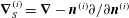 $\unicode[STIX]{x1D735}_{S}^{(i)}=\unicode[STIX]{x1D735}-\boldsymbol{n}^{(i)}\unicode[STIX]{x2202}/\unicode[STIX]{x2202}\boldsymbol{n}^{(i)}$
is the surface gradient on the
$\unicode[STIX]{x1D735}_{S}^{(i)}=\unicode[STIX]{x1D735}-\boldsymbol{n}^{(i)}\unicode[STIX]{x2202}/\unicode[STIX]{x2202}\boldsymbol{n}^{(i)}$
is the surface gradient on the
 $i$
th boundary. At the exit of the device the speed of the (now solid) thread is controlled by the take-up roller and hence given by
$i$
th boundary. At the exit of the device the speed of the (now solid) thread is controlled by the take-up roller and hence given by
 $u=U_{out}$
and
$u=U_{out}$
and
 $v=w=0$
at
$v=w=0$
at
 $x=L$
.
$x=L$
.
The governing equation for the temperature
 $\unicode[STIX]{x1D703}$
is given by
$\unicode[STIX]{x1D703}$
is given by
 $$\begin{eqnarray}\displaystyle \unicode[STIX]{x1D70C}c_{p}\left(\frac{\unicode[STIX]{x2202}\unicode[STIX]{x1D703}}{\unicode[STIX]{x2202}t}+\boldsymbol{u}\boldsymbol{\cdot }\unicode[STIX]{x1D735}\unicode[STIX]{x1D703}\right)=k\unicode[STIX]{x1D6FB}^{2}\unicode[STIX]{x1D703}, & & \displaystyle\end{eqnarray}$$
where
 $c_{p}$
and
$c_{p}$
and
 $k$
are the specific heat and conductivity of the glass, respectively. Here we have neglected the effects of radiative heat penetrating into the interior of the glass. This is because the glass can be approximated as being optically thick for wavelengths that dominate the radiative heat transfer (Modest Reference Modest2013). Radiative heating is therefore assumed to occur only at the external boundary of the thread. At the external boundary, the thread is also cooled by blowing cold gas through the device. Hence we have the boundary condition
$k$
are the specific heat and conductivity of the glass, respectively. Here we have neglected the effects of radiative heat penetrating into the interior of the glass. This is because the glass can be approximated as being optically thick for wavelengths that dominate the radiative heat transfer (Modest Reference Modest2013). Radiative heating is therefore assumed to occur only at the external boundary of the thread. At the external boundary, the thread is also cooled by blowing cold gas through the device. Hence we have the boundary condition
 $$\begin{eqnarray}\displaystyle -k\unicode[STIX]{x1D735}\unicode[STIX]{x1D703}\boldsymbol{\cdot }\boldsymbol{n}^{(0)}=F_{R}(\unicode[STIX]{x1D703})+F_{C}(\unicode[STIX]{x1D703}),\quad \text{on }G^{(0)}(\boldsymbol{x},t)=0, & & \displaystyle\end{eqnarray}$$
where
 $F_{R}(\unicode[STIX]{x1D703})$
and
$F_{R}(\unicode[STIX]{x1D703})$
and
 $F_{C}(\unicode[STIX]{x1D703})$
are the radiative and convective heat transfer rates, respectively. We will assume that
$F_{C}(\unicode[STIX]{x1D703})$
are the radiative and convective heat transfer rates, respectively. We will assume that
 $F_{R}$
is given by
$F_{R}$
is given by
 $$\begin{eqnarray}\displaystyle F_{R}(\unicode[STIX]{x1D703},x)=\left\{\begin{array}{@{}ll@{}}k_{b}\unicode[STIX]{x1D6FD}(\unicode[STIX]{x1D703}^{4}-\unicode[STIX]{x1D703}_{h}^{4}(x)),\quad & 0\leqslant x\leqslant L_{h},\\ k_{b}\unicode[STIX]{x1D6FD}(\unicode[STIX]{x1D703}^{4}-\unicode[STIX]{x1D703}_{a}^{4}),\quad & L_{h}<x\leqslant L,\end{array}\right. & & \displaystyle\end{eqnarray}$$
where
 $k_{b}$
is the Stefan–Boltzmann constant,
$k_{b}$
is the Stefan–Boltzmann constant,
 $\unicode[STIX]{x1D6FD}$
is the absorptivity of the glass surface,
$\unicode[STIX]{x1D6FD}$
is the absorptivity of the glass surface,
 $\unicode[STIX]{x1D703}_{a}$
is the ambient temperature and
$\unicode[STIX]{x1D703}_{a}$
is the ambient temperature and
 $\unicode[STIX]{x1D703}_{h}(x)$
is the effective temperature of the heater that, in general, will be spatially dependent. We will further assume that
$\unicode[STIX]{x1D703}_{h}(x)$
is the effective temperature of the heater that, in general, will be spatially dependent. We will further assume that
 $F_{C}$
is given by
$F_{C}$
is given by
 $$\begin{eqnarray}\displaystyle F_{C}(\unicode[STIX]{x1D703})=h_{w}(\unicode[STIX]{x1D703}-\unicode[STIX]{x1D703}_{a}), & & \displaystyle\end{eqnarray}$$
where
 $h_{w}$
is the heat transfer coefficient for convective gas flow and the temperature of the gas is assumed to be the same as the ambient temperature. In writing down (2.2c
), we have assumed that the ambient temperature is a constant. We will assume that radiative heat transfer across internal cavities will be negligible compared to the heat transfer from the external boundary and, thus, we assume that
$h_{w}$
is the heat transfer coefficient for convective gas flow and the temperature of the gas is assumed to be the same as the ambient temperature. In writing down (2.2c
), we have assumed that the ambient temperature is a constant. We will assume that radiative heat transfer across internal cavities will be negligible compared to the heat transfer from the external boundary and, thus, we assume that
 $$\begin{eqnarray}\displaystyle -k\unicode[STIX]{x1D735}\unicode[STIX]{x1D703}\boldsymbol{\cdot }\boldsymbol{n}^{(i)}=0,\quad \text{on }G^{(i)}(\boldsymbol{x},t)=0,i\neq 0. & & \displaystyle\end{eqnarray}$$
This assumption is reasonable in the case that there is no significant cooling arising from any gas flow through the internal cavities (which is here assumed to be negligible). At the aperture the temperature is specified,
 $$\begin{eqnarray}\displaystyle \unicode[STIX]{x1D703}=\unicode[STIX]{x1D703}_{in},\quad \text{at }x=0. & & \displaystyle\end{eqnarray}$$
In principle, we also need to specify a boundary condition on the temperature at the take-up roller. The exact details of this condition will depend on the nature of the take-up roller. We will later show that the axial conduction terms are small and that for our purposes such a condition is not required.
The theory we will develop will be appropriate for arbitrary viscosity–temperature and surface tension–temperature relations. However, for definiteness, we will use the following empirical relations that have been widely used in the literature. We will assume that the viscosity–temperature relation is given by the Vogel–Fulcher–Tamann (VFT) equation (Scherer Reference Scherer1992) with parameters obtained by empirically fitting using the data for F2 glass (K. Richardson, 2012, private communication as part of NSF-DMR #0807016 ‘Materials world network in advanced optical glasses for novel optical fibers’),
 $$\begin{eqnarray}\displaystyle \log _{10}\unicode[STIX]{x1D707}=-2.314+\frac{4065.2}{\unicode[STIX]{x1D703}-410.15}, & & \displaystyle\end{eqnarray}$$
where the temperature
 $\unicode[STIX]{x1D703}$
is measured in Kelvin and
$\unicode[STIX]{x1D703}$
is measured in Kelvin and
 $\unicode[STIX]{x1D707}$
is given in Pa s. The relation between the surface-tension coefficient of F2 glass and temperature can be fitted using the data in Boyd et al. (Reference Boyd, Ebendorff-Heidepriem, Monro and Munch2012) to give
$\unicode[STIX]{x1D707}$
is given in Pa s. The relation between the surface-tension coefficient of F2 glass and temperature can be fitted using the data in Boyd et al. (Reference Boyd, Ebendorff-Heidepriem, Monro and Munch2012) to give
 $$\begin{eqnarray}\displaystyle \unicode[STIX]{x1D6FE}=0.23(1-2\times 10^{-4}(\unicode[STIX]{x1D703}-1373)), & & \displaystyle\end{eqnarray}$$
where the surface tension is measured in
 $\text{N}~\text{m}^{-1}$
. This magnitude of variation is also broadly consistent with the data of Shartsis & Spinner (Reference Shartsis and Spinner1951) for a wide range of silica glasses.
$\text{N}~\text{m}^{-1}$
. This magnitude of variation is also broadly consistent with the data of Shartsis & Spinner (Reference Shartsis and Spinner1951) for a wide range of silica glasses.
2.2 Scaling and slenderness approximation for the steady state problem
There are some subtleties that one must take into account when choosing scales for non-dimensionalisation. In particular, when selecting a scale for the viscosity, we are faced with the issue that the viscosity of the glass varies by many orders of magnitude as the temperature changes. In order to select an appropriate scale, one should select a viscosity at which the majority of the deformation occurs. This is clearly not the input temperature at which the viscosity is extremely high. However, it is also not the viscosity associated with the temperature of the radiative heater because the convective cooling means that the maximum temperature the thread can attain is significantly lower than the radiative heater temperature. Therefore, a useful quantity is the temperature at which heating from the radiative source (at the location with the strongest heating) balances the convective cooling. We denote this temperature as
 $\unicode[STIX]{x1D703}_{hot}$
which, from (2.2b
), is given by solving the equation
$\unicode[STIX]{x1D703}_{hot}$
which, from (2.2b
), is given by solving the equation
 $$\begin{eqnarray}\displaystyle k_{b}\unicode[STIX]{x1D6FD}(\unicode[STIX]{x1D703}_{hot}^{4}-\max _{x}\{\unicode[STIX]{x1D703}_{h}^{4}(x)\})+h_{w}(\unicode[STIX]{x1D703}_{hot}-\unicode[STIX]{x1D703}_{a})=0. & & \displaystyle\end{eqnarray}$$
Thus,
 $\unicode[STIX]{x1D703}_{hot}$
represents the maximum temperature that the glass would achieve if it were placed in the heater and allowed to reach equilibrium. We then use this value of the temperature to define
$\unicode[STIX]{x1D703}_{hot}$
represents the maximum temperature that the glass would achieve if it were placed in the heater and allowed to reach equilibrium. We then use this value of the temperature to define
 $\unicode[STIX]{x1D707}_{hot}=\unicode[STIX]{x1D707}(\unicode[STIX]{x1D703}_{hot})$
which we will choose as our viscosity scale. Table 1 shows typical parameter values for fibre drawing assuming the preform material is F2 glass, a commercial lead-silicate glass from the Schott Glass Company whose physical properties are provided in the company’s Optical Glass – Collection Data Sheets (https://www.schott.com/advanced_optics/english/download/index.html). Other parameter values are consistent with experiments performed in the Institute for Photonics and Advanced Sensing (IPAS) at The University of Adelaide. Using these values and solving the above quartic equation we obtain
$\unicode[STIX]{x1D707}_{hot}=\unicode[STIX]{x1D707}(\unicode[STIX]{x1D703}_{hot})$
which we will choose as our viscosity scale. Table 1 shows typical parameter values for fibre drawing assuming the preform material is F2 glass, a commercial lead-silicate glass from the Schott Glass Company whose physical properties are provided in the company’s Optical Glass – Collection Data Sheets (https://www.schott.com/advanced_optics/english/download/index.html). Other parameter values are consistent with experiments performed in the Institute for Photonics and Advanced Sensing (IPAS) at The University of Adelaide. Using these values and solving the above quartic equation we obtain
 $\unicode[STIX]{x1D703}_{hot}\approx 1020~\text{K}$
and
$\unicode[STIX]{x1D703}_{hot}\approx 1020~\text{K}$
and
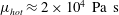 $\unicode[STIX]{x1D707}_{hot}\approx 2\times 10^{4}~\text{Pa}~\text{s}$
. This means that the viscosity varies by approximately 10 orders of magnitude over
$\unicode[STIX]{x1D707}_{hot}\approx 2\times 10^{4}~\text{Pa}~\text{s}$
. This means that the viscosity varies by approximately 10 orders of magnitude over
 $\unicode[STIX]{x1D703}_{in}\leqslant \unicode[STIX]{x1D703}\leqslant \unicode[STIX]{x1D703}_{hot}$
. Although the variation of surface tension with temperature is much less dramatic (typically approximately 5–10 %), it can still be significant in affecting the evolution of the shape of the thread. We choose
$\unicode[STIX]{x1D703}_{in}\leqslant \unicode[STIX]{x1D703}\leqslant \unicode[STIX]{x1D703}_{hot}$
. Although the variation of surface tension with temperature is much less dramatic (typically approximately 5–10 %), it can still be significant in affecting the evolution of the shape of the thread. We choose
 $\unicode[STIX]{x1D6FE}_{hot}=\unicode[STIX]{x1D6FE}(\unicode[STIX]{x1D703}_{hot})\approx 0.24~\text{N}~\text{m}^{-1}$
as a typical scale for the surface tension.
$\unicode[STIX]{x1D6FE}_{hot}=\unicode[STIX]{x1D6FE}(\unicode[STIX]{x1D703}_{hot})\approx 0.24~\text{N}~\text{m}^{-1}$
as a typical scale for the surface tension.
Table 1. Typical parameters for drawing a fibre from a preform made from F2 glass.

Moreover, draw towers tend to be a few metres in length, but for the vast majority of this length, the thread will be sufficiently cool that the viscosity will be much too high for any meaningful deformation to occur. We therefore choose the axial length scale to be a length beyond which no significant deformation occurs and denote this as
 $L$
. For convenience, we non-dimensionalise the radial length scales using
$L$
. For convenience, we non-dimensionalise the radial length scales using
 $\unicode[STIX]{x1D712}_{in}$
that represents the square root of the cross-sectional area. With these issues in mind, we select the following scales
$\unicode[STIX]{x1D712}_{in}$
that represents the square root of the cross-sectional area. With these issues in mind, we select the following scales
 $$\begin{eqnarray}\left.\begin{array}{@{}c@{}}(x,y,z)=L(x^{\prime },\unicode[STIX]{x1D716}y^{\prime },\unicode[STIX]{x1D716}z^{\prime }),\quad t={\displaystyle \frac{L}{U_{in}}}t^{\prime },\quad p={\displaystyle \frac{\unicode[STIX]{x1D707}_{hot}U_{in}}{L}}p^{\prime },\\ (u,v,w)=U_{in}(u^{\prime },\unicode[STIX]{x1D716}v^{\prime },\unicode[STIX]{x1D716}w^{\prime }),\quad \unicode[STIX]{x1D712}=\unicode[STIX]{x1D712}_{in}\unicode[STIX]{x1D712}^{\prime },\quad \unicode[STIX]{x1D6E4}=\unicode[STIX]{x1D712}_{in}\unicode[STIX]{x1D6E4}^{\prime },\quad \unicode[STIX]{x1D705}=\unicode[STIX]{x1D705}^{\prime }/\unicode[STIX]{x1D712}_{in},\\ \unicode[STIX]{x1D703}=\unicode[STIX]{x1D703}_{in}+\unicode[STIX]{x1D6E9}\unicode[STIX]{x1D703}^{\prime },\quad \unicode[STIX]{x1D707}(\unicode[STIX]{x1D703})=\unicode[STIX]{x1D707}_{hot}\unicode[STIX]{x1D707}^{\prime }(\unicode[STIX]{x1D703}^{\prime }),\quad \unicode[STIX]{x1D6FE}=\unicode[STIX]{x1D6FE}_{hot}\unicode[STIX]{x1D6FE}^{\prime }(\unicode[STIX]{x1D703}^{\prime }),\end{array}\right\}\end{eqnarray}$$
where
 $\unicode[STIX]{x1D6E9}=(\unicode[STIX]{x1D703}_{hot}-\unicode[STIX]{x1D703}_{in})$
and primes denote dimensionless variables.
$\unicode[STIX]{x1D6E9}=(\unicode[STIX]{x1D703}_{hot}-\unicode[STIX]{x1D703}_{in})$
and primes denote dimensionless variables.
We next consider the steady-state equations by setting
 $\unicode[STIX]{x2202}_{t}\equiv 0$
, substitute the above scalings into the governing equations and drop the primes for convenience. The momentum equation (2.1b
) yields
$\unicode[STIX]{x2202}_{t}\equiv 0$
, substitute the above scalings into the governing equations and drop the primes for convenience. The momentum equation (2.1b
) yields
 $$\begin{eqnarray}\displaystyle & & \displaystyle \mathit{Re}\,\unicode[STIX]{x1D716}^{2}\left(u\frac{\unicode[STIX]{x2202}u}{\unicode[STIX]{x2202}x}+v\frac{\unicode[STIX]{x2202}u}{\unicode[STIX]{x2202}y}+w\frac{\unicode[STIX]{x2202}u}{\unicode[STIX]{x2202}z}\right)=-\unicode[STIX]{x1D716}^{2}\frac{\unicode[STIX]{x2202}p}{\unicode[STIX]{x2202}x}\nonumber\\ \displaystyle & & \displaystyle \quad +\,\unicode[STIX]{x1D716}^{2}\frac{\unicode[STIX]{x2202}}{\unicode[STIX]{x2202}x}\left(2\unicode[STIX]{x1D707}\frac{\unicode[STIX]{x2202}u}{\unicode[STIX]{x2202}x}\right)+\frac{\unicode[STIX]{x2202}}{\unicode[STIX]{x2202}y}\left(\unicode[STIX]{x1D707}\left[\frac{\unicode[STIX]{x2202}u}{\unicode[STIX]{x2202}y}+\unicode[STIX]{x1D716}^{2}\frac{\unicode[STIX]{x2202}v}{\unicode[STIX]{x2202}x}\right]\right)+\frac{\unicode[STIX]{x2202}}{\unicode[STIX]{x2202}z}\left(\unicode[STIX]{x1D707}\left[\frac{\unicode[STIX]{x2202}u}{\unicode[STIX]{x2202}z}+\unicode[STIX]{x1D716}^{2}\frac{\unicode[STIX]{x2202}w}{\unicode[STIX]{x2202}x}\right]\right),\quad\end{eqnarray}$$
 $$\begin{eqnarray}\displaystyle & & \displaystyle \mathit{Re}\,\unicode[STIX]{x1D716}^{2}\left(u\frac{\unicode[STIX]{x2202}v}{\unicode[STIX]{x2202}x}+v\frac{\unicode[STIX]{x2202}v}{\unicode[STIX]{x2202}y}+w\frac{\unicode[STIX]{x2202}v}{\unicode[STIX]{x2202}z}\right)=-\frac{\unicode[STIX]{x2202}p}{\unicode[STIX]{x2202}y}\nonumber\\ \displaystyle & & \displaystyle \quad +\,\frac{\unicode[STIX]{x2202}}{\unicode[STIX]{x2202}x}\left(\unicode[STIX]{x1D707}\left[\unicode[STIX]{x1D716}^{2}\frac{\unicode[STIX]{x2202}v}{\unicode[STIX]{x2202}x}+\frac{\unicode[STIX]{x2202}u}{\unicode[STIX]{x2202}y}\right]\right)+\frac{\unicode[STIX]{x2202}}{\unicode[STIX]{x2202}y}\left(2\unicode[STIX]{x1D707}\frac{\unicode[STIX]{x2202}v}{\unicode[STIX]{x2202}y}\right)+\frac{\unicode[STIX]{x2202}}{\unicode[STIX]{x2202}z}\left(\unicode[STIX]{x1D707}\left[\frac{\unicode[STIX]{x2202}v}{\unicode[STIX]{x2202}z}+\frac{\unicode[STIX]{x2202}w}{\unicode[STIX]{x2202}y}\right]\right),\end{eqnarray}$$
 $$\begin{eqnarray}\displaystyle & & \displaystyle \mathit{Re}\,\unicode[STIX]{x1D716}^{2}\left(u\frac{\unicode[STIX]{x2202}w}{\unicode[STIX]{x2202}x}+v\frac{\unicode[STIX]{x2202}w}{\unicode[STIX]{x2202}y}+w\frac{\unicode[STIX]{x2202}w}{\unicode[STIX]{x2202}z}\right)=-\frac{\unicode[STIX]{x2202}p}{\unicode[STIX]{x2202}z}\nonumber\\ \displaystyle & & \displaystyle \quad +\,\frac{\unicode[STIX]{x2202}}{\unicode[STIX]{x2202}x}\left(\unicode[STIX]{x1D707}\left[\unicode[STIX]{x1D716}^{2}\frac{\unicode[STIX]{x2202}w}{\unicode[STIX]{x2202}x}+\frac{\unicode[STIX]{x2202}u}{\unicode[STIX]{x2202}z}\right]\right)+\frac{\unicode[STIX]{x2202}}{\unicode[STIX]{x2202}y}\left(\unicode[STIX]{x1D707}\left[\frac{\unicode[STIX]{x2202}w}{\unicode[STIX]{x2202}y}+\frac{\unicode[STIX]{x2202}v}{\unicode[STIX]{x2202}z}\right]\right)+\frac{\unicode[STIX]{x2202}}{\unicode[STIX]{x2202}z}\left(2\unicode[STIX]{x1D707}\frac{\unicode[STIX]{x2202}w}{\unicode[STIX]{x2202}z}\right),\end{eqnarray}$$
 $$\begin{eqnarray}\displaystyle \unicode[STIX]{x1D716}=\frac{\unicode[STIX]{x1D712}_{in}}{L}, & & \displaystyle\end{eqnarray}$$
is the slenderness parameter and
 $$\begin{eqnarray}\displaystyle \mathit{Re}=\frac{\unicode[STIX]{x1D70C}U_{in}L}{\unicode[STIX]{x1D707}_{hot}}, & & \displaystyle\end{eqnarray}$$
is the Reynolds number. The continuity equation (2.1a ) yields
 $$\begin{eqnarray}\displaystyle \frac{\unicode[STIX]{x2202}u}{\unicode[STIX]{x2202}x}+\frac{\unicode[STIX]{x2202}v}{\unicode[STIX]{x2202}y}+\frac{\unicode[STIX]{x2202}w}{\unicode[STIX]{x2202}z}=0. & & \displaystyle\end{eqnarray}$$
The boundary conditions (2.1c ) are given by
 $$\begin{eqnarray}\displaystyle & & \displaystyle \unicode[STIX]{x1D716}^{2}\left(-p+2\unicode[STIX]{x1D707}\frac{\unicode[STIX]{x2202}u}{\unicode[STIX]{x2202}x}\right)n_{x}^{(i)}+\unicode[STIX]{x1D707}\left(\frac{\unicode[STIX]{x2202}u}{\unicode[STIX]{x2202}y}+\unicode[STIX]{x1D716}^{2}\frac{\unicode[STIX]{x2202}v}{\unicode[STIX]{x2202}x}\right)n_{y}^{(i)}+\unicode[STIX]{x1D707}\left(\frac{\unicode[STIX]{x2202}u}{\unicode[STIX]{x2202}z}+\unicode[STIX]{x1D716}^{2}\frac{\unicode[STIX]{x2202}w}{\unicode[STIX]{x2202}x}\right)n_{z}^{(i)}\nonumber\\ \displaystyle & & \displaystyle \quad =\frac{\unicode[STIX]{x1D716}^{2}}{\mathit{Ca}}\left(-\unicode[STIX]{x1D6FE}\unicode[STIX]{x1D705}^{(i)}n_{x}^{(i)}+\frac{\unicode[STIX]{x2202}\unicode[STIX]{x1D6FE}}{\unicode[STIX]{x2202}x}-\left[\unicode[STIX]{x1D716}^{2}\frac{\unicode[STIX]{x2202}\unicode[STIX]{x1D6FE}}{\unicode[STIX]{x2202}x}n_{x}^{(i)}+\frac{\unicode[STIX]{x2202}\unicode[STIX]{x1D6FE}}{\unicode[STIX]{x2202}y}n_{y}^{(i)}+\frac{\unicode[STIX]{x2202}\unicode[STIX]{x1D6FE}}{\unicode[STIX]{x2202}z}n_{z}^{(i)}\right]n_{x}^{(i)}\right),\quad\end{eqnarray}$$
 $$\begin{eqnarray}\displaystyle & & \displaystyle \left(-p+2\unicode[STIX]{x1D707}\frac{\unicode[STIX]{x2202}v}{\unicode[STIX]{x2202}y}\right)n_{y}^{(i)}+\unicode[STIX]{x1D707}\left(\unicode[STIX]{x1D716}^{2}\frac{\unicode[STIX]{x2202}v}{\unicode[STIX]{x2202}x}+\frac{\unicode[STIX]{x2202}u}{\unicode[STIX]{x2202}y}\right)n_{x}^{(i)}+\unicode[STIX]{x1D707}\left(\frac{\unicode[STIX]{x2202}v}{\unicode[STIX]{x2202}z}+\frac{\unicode[STIX]{x2202}w}{\unicode[STIX]{x2202}y}\right)n_{z}^{(i)}\nonumber\\ \displaystyle & & \displaystyle \quad =\frac{1}{\mathit{Ca}}\left(-\unicode[STIX]{x1D6FE}\unicode[STIX]{x1D705}^{(i)}n_{y}^{(i)}+\frac{\unicode[STIX]{x2202}\unicode[STIX]{x1D6FE}}{\unicode[STIX]{x2202}y}-\left[\unicode[STIX]{x1D716}^{2}\frac{\unicode[STIX]{x2202}\unicode[STIX]{x1D6FE}}{\unicode[STIX]{x2202}x}n_{x}^{(i)}+\frac{\unicode[STIX]{x2202}\unicode[STIX]{x1D6FE}}{\unicode[STIX]{x2202}y}n_{y}^{(i)}+\frac{\unicode[STIX]{x2202}\unicode[STIX]{x1D6FE}}{\unicode[STIX]{x2202}z}n_{z}^{(i)}\right]n_{y}^{(i)}\right),\end{eqnarray}$$
 $$\begin{eqnarray}\displaystyle & & \displaystyle \left(-p+2\unicode[STIX]{x1D707}\frac{\unicode[STIX]{x2202}w}{\unicode[STIX]{x2202}z}\right)n_{z}^{(i)}+\unicode[STIX]{x1D707}\left(\unicode[STIX]{x1D716}^{2}\frac{\unicode[STIX]{x2202}w}{\unicode[STIX]{x2202}x}+\frac{\unicode[STIX]{x2202}u}{\unicode[STIX]{x2202}z}\right)n_{x}^{(i)}+\unicode[STIX]{x1D707}\left(\frac{\unicode[STIX]{x2202}v}{\unicode[STIX]{x2202}z}+\frac{\unicode[STIX]{x2202}w}{\unicode[STIX]{x2202}y}\right)n_{y}^{(i)}\nonumber\\ \displaystyle & & \displaystyle \quad =\frac{1}{\mathit{Ca}}\left(-\unicode[STIX]{x1D6FE}\unicode[STIX]{x1D705}^{(i)}n_{z}^{(i)}+\frac{\unicode[STIX]{x2202}\unicode[STIX]{x1D6FE}}{\unicode[STIX]{x2202}z}-\left[\unicode[STIX]{x1D716}^{2}\frac{\unicode[STIX]{x2202}\unicode[STIX]{x1D6FE}}{\unicode[STIX]{x2202}x}n_{x}^{(i)}+\frac{\unicode[STIX]{x2202}\unicode[STIX]{x1D6FE}}{\unicode[STIX]{x2202}y}n_{y}^{(i)}+\frac{\unicode[STIX]{x2202}\unicode[STIX]{x1D6FE}}{\unicode[STIX]{x2202}z}n_{z}^{(i)}\right]n_{z}^{(i)}\right),\end{eqnarray}$$
 $$\begin{eqnarray}\displaystyle \mathit{Ca}=\frac{\unicode[STIX]{x1D707}_{hot}U_{in}\unicode[STIX]{x1D712}_{in}}{\unicode[STIX]{x1D6FE}_{hot}L}, & & \displaystyle\end{eqnarray}$$
is the effective capillary number and it is understood that
 $\unicode[STIX]{x1D6FE}$
is a function of
$\unicode[STIX]{x1D6FE}$
is a function of
 $\unicode[STIX]{x1D703}(x,y,z)$
. Note that the constant dimensionless surface-tension parameter
$\unicode[STIX]{x1D703}(x,y,z)$
. Note that the constant dimensionless surface-tension parameter
 $\unicode[STIX]{x1D6FE}^{\ast }$
defined in Stokes et al. (Reference Stokes, Buchak, Crowdy and Ebendorff-Heidepriem2014) is a function of
$\unicode[STIX]{x1D6FE}^{\ast }$
defined in Stokes et al. (Reference Stokes, Buchak, Crowdy and Ebendorff-Heidepriem2014) is a function of
 $\unicode[STIX]{x1D703}$
for temperature-dependent surface tension, and
$\unicode[STIX]{x1D703}$
for temperature-dependent surface tension, and
 $$\begin{eqnarray}\displaystyle \unicode[STIX]{x1D6FE}^{\ast }(\unicode[STIX]{x1D703})\equiv \frac{\unicode[STIX]{x1D6FE}(\unicode[STIX]{x1D703})}{\mathit{Ca}}, & & \displaystyle\end{eqnarray}$$
in the notation of this paper. The steady-state kinematic conditions (2.1d ) are invariant under the scaling and are hence given by
 $$\begin{eqnarray}\displaystyle u\frac{\unicode[STIX]{x2202}G^{(i)}}{\unicode[STIX]{x2202}x}+v\frac{\unicode[STIX]{x2202}G^{(i)}}{\unicode[STIX]{x2202}y}+w\frac{\unicode[STIX]{x2202}G^{(i)}}{\unicode[STIX]{x2202}z}=0. & & \displaystyle\end{eqnarray}$$
The boundary conditions at the aperture
 $x=0$
are given by
$x=0$
are given by
 $$\begin{eqnarray}\displaystyle u=1,\quad v=w=0,\quad \text{and}\quad \unicode[STIX]{x1D712}=1, & & \displaystyle\end{eqnarray}$$
whereas the boundary conditions at the take-up roller and, hence, at
 $x=1$
, are given by
$x=1$
, are given by
 $$\begin{eqnarray}\displaystyle u=D,\quad v=w=0, & & \displaystyle\end{eqnarray}$$
where
 $$\begin{eqnarray}\displaystyle D=\frac{U_{out}}{U_{in}}, & & \displaystyle\end{eqnarray}$$
is the draw ratio.
The steady-state energy conservation equation (2.2a ) takes the form
 $$\begin{eqnarray}\displaystyle \unicode[STIX]{x1D716}^{2}\mathit{Pe}\left(u\frac{\unicode[STIX]{x2202}\unicode[STIX]{x1D703}}{\unicode[STIX]{x2202}x}+v\frac{\unicode[STIX]{x2202}\unicode[STIX]{x1D703}}{\unicode[STIX]{x2202}y}+w\frac{\unicode[STIX]{x2202}\unicode[STIX]{x1D703}}{\unicode[STIX]{x2202}z}\right)=\unicode[STIX]{x1D716}^{2}\frac{\unicode[STIX]{x2202}^{2}\unicode[STIX]{x1D703}}{\unicode[STIX]{x2202}x^{2}}+\frac{\unicode[STIX]{x2202}^{2}\unicode[STIX]{x1D703}}{\unicode[STIX]{x2202}y^{2}}+\frac{\unicode[STIX]{x2202}^{2}\unicode[STIX]{x1D703}}{\unicode[STIX]{x2202}z^{2}}, & & \displaystyle\end{eqnarray}$$
where
 $$\begin{eqnarray}\displaystyle \mathit{Pe}=\frac{\unicode[STIX]{x1D70C}c_{p}U_{in}L}{k}, & & \displaystyle\end{eqnarray}$$
is the Péclet number. The boundary condition on the external surface of the thread (2.2b ) becomes
 $$\begin{eqnarray}\displaystyle -\left(\unicode[STIX]{x1D716}^{2}\frac{\unicode[STIX]{x2202}\unicode[STIX]{x1D703}}{\unicode[STIX]{x2202}x}n_{x}^{(0)}+\unicode[STIX]{x1D735}_{\bot }\unicode[STIX]{x1D703}\boldsymbol{\cdot }\boldsymbol{n}_{\bot }^{(0)}\right)=\frac{\unicode[STIX]{x1D716}^{2}\mathit{Pe}}{\mathit{Ca}}[{\mathcal{H}}_{R}f_{R}(\unicode[STIX]{x1D703},x)+{\mathcal{H}}_{C}f_{C}(\unicode[STIX]{x1D703})], & & \displaystyle\end{eqnarray}$$
where
 $$\begin{eqnarray}\displaystyle {\mathcal{H}}_{R}=\frac{\unicode[STIX]{x1D6FD}k_{b}\unicode[STIX]{x1D703}_{hot}^{4}\unicode[STIX]{x1D707}_{hot}}{\unicode[STIX]{x1D70C}c_{p}\unicode[STIX]{x1D6E9}\unicode[STIX]{x1D6FE}_{hot}},\quad \text{and}\quad {\mathcal{H}}_{C}=\frac{h_{w}\unicode[STIX]{x1D703}_{hot}\unicode[STIX]{x1D707}_{hot}}{\unicode[STIX]{x1D70C}c_{p}\unicode[STIX]{x1D6E9}\unicode[STIX]{x1D6FE}_{hot}}, & & \displaystyle\end{eqnarray}$$
are the dimensionless parameters that represent the importance of radiative and convective cooling, respectively. Here,
 $\unicode[STIX]{x1D735}_{\bot }=(\unicode[STIX]{x2202}/\unicode[STIX]{x2202}y,\unicode[STIX]{x2202}/\unicode[STIX]{x2202}z)$
,
$\unicode[STIX]{x1D735}_{\bot }=(\unicode[STIX]{x2202}/\unicode[STIX]{x2202}y,\unicode[STIX]{x2202}/\unicode[STIX]{x2202}z)$
,
 $\boldsymbol{n}_{\bot }^{(i)}=(n_{y}^{(i)},n_{z}^{(i)})$
,
$\boldsymbol{n}_{\bot }^{(i)}=(n_{y}^{(i)},n_{z}^{(i)})$
,
 $$\begin{eqnarray}\displaystyle f_{C}(\unicode[STIX]{x1D703})=(1-\unicode[STIX]{x1D717}_{in})\unicode[STIX]{x1D703}+\unicode[STIX]{x1D717}_{in}-\unicode[STIX]{x1D717}_{a}, & & \displaystyle\end{eqnarray}$$
and
 $$\begin{eqnarray}\displaystyle f_{R}(\unicode[STIX]{x1D703},x)=\left\{\begin{array}{@{}ll@{}}(\unicode[STIX]{x1D703}+\unicode[STIX]{x1D717}_{in}(1-\unicode[STIX]{x1D703}))^{4}-(\unicode[STIX]{x1D717}_{h}(x))^{4},\quad & 0\leqslant x\leqslant \ell ,\\ (\unicode[STIX]{x1D703}+\unicode[STIX]{x1D717}_{in}(1-\unicode[STIX]{x1D703}))^{4}-\unicode[STIX]{x1D717}_{a}^{4},\quad & \ell <x\leqslant 1,\end{array}\right. & & \displaystyle\end{eqnarray}$$
where
 $$\begin{eqnarray}\displaystyle \unicode[STIX]{x1D717}_{in}=\frac{\unicode[STIX]{x1D703}_{in}}{\unicode[STIX]{x1D703}_{hot}},\quad \unicode[STIX]{x1D717}_{a}=\frac{\unicode[STIX]{x1D703}_{a}}{\unicode[STIX]{x1D703}_{hot}},\quad \text{and}\quad \unicode[STIX]{x1D717}_{h}(x)=\frac{\unicode[STIX]{x1D703}_{h}(x)}{\unicode[STIX]{x1D703}_{hot}}, & & \displaystyle\end{eqnarray}$$
are the input glass, ambient air and heater temperatures scaled with
 $\unicode[STIX]{x1D703}_{hot}$
, and
$\unicode[STIX]{x1D703}_{hot}$
, and
 $$\begin{eqnarray}\displaystyle \ell =L_{h}/L, & & \displaystyle\end{eqnarray}$$
is the dimensionless length of the heater. On internal air-channel surfaces the boundary condition (2.2e ) is given by
 $$\begin{eqnarray}\displaystyle -\left(\unicode[STIX]{x1D716}^{2}\frac{\unicode[STIX]{x2202}\unicode[STIX]{x1D703}}{\unicode[STIX]{x2202}x}n_{x}^{(i)}+\unicode[STIX]{x1D735}_{\bot }\unicode[STIX]{x1D703}\boldsymbol{\cdot }\boldsymbol{n}_{\bot }^{(i)}\right)=0. & & \displaystyle\end{eqnarray}$$
From the typical parameter values for fibre drawing given in table 1, we see that
 $\unicode[STIX]{x1D716}=O(10^{-1})$
. As is typical in the modelling of fibre drawing problems (Yarin et al.
Reference Yarin, Rusinov and Gospodinov1989; Dewynne et al.
Reference Dewynne, Howell and Wilmott1994; Cummings & Howell Reference Cummings and Howell1999; Stokes et al.
Reference Stokes, Tuck and Schwartz2000, Reference Stokes, Buchak, Crowdy and Ebendorff-Heidepriem2014; Fitt et al.
Reference Fitt, Furusawa, Monro, Please and Richardson2002; Wylie et al.
Reference Wylie, Huang and Miura2007; Griffiths & Howell Reference Griffiths and Howell2008; Taroni et al.
Reference Taroni, Breward, Cummings and Griffiths2013), we exploit the fact that
$\unicode[STIX]{x1D716}=O(10^{-1})$
. As is typical in the modelling of fibre drawing problems (Yarin et al.
Reference Yarin, Rusinov and Gospodinov1989; Dewynne et al.
Reference Dewynne, Howell and Wilmott1994; Cummings & Howell Reference Cummings and Howell1999; Stokes et al.
Reference Stokes, Tuck and Schwartz2000, Reference Stokes, Buchak, Crowdy and Ebendorff-Heidepriem2014; Fitt et al.
Reference Fitt, Furusawa, Monro, Please and Richardson2002; Wylie et al.
Reference Wylie, Huang and Miura2007; Griffiths & Howell Reference Griffiths and Howell2008; Taroni et al.
Reference Taroni, Breward, Cummings and Griffiths2013), we exploit the fact that
 $\unicode[STIX]{x1D716}\ll 1$
to develop long-wavelength equations that are significantly simpler to deal with than the full equations given above. Thus, we expand all dependent variables in powers of
$\unicode[STIX]{x1D716}\ll 1$
to develop long-wavelength equations that are significantly simpler to deal with than the full equations given above. Thus, we expand all dependent variables in powers of
 $\unicode[STIX]{x1D716}^{2}$
,
$\unicode[STIX]{x1D716}^{2}$
,
 $$\begin{eqnarray}\displaystyle \left.\begin{array}{@{}c@{}}\unicode[STIX]{x1D703}=\unicode[STIX]{x1D703}_{0}(x,y,z)+\unicode[STIX]{x1D716}^{2}\unicode[STIX]{x1D703}_{1}(x,y,z)+\unicode[STIX]{x1D716}^{4}\unicode[STIX]{x1D703}_{2}(x,y,z)+\cdots \,,\\ u=u_{0}(x,y,z)+\unicode[STIX]{x1D716}^{2}u_{1}(x,y,z)+\unicode[STIX]{x1D716}^{4}u_{2}(x,y,z)+\cdots \,,\end{array}\right\} & & \displaystyle\end{eqnarray}$$
and similarly for
 $v$
,
$v$
,
 $w$
,
$w$
,
 $p$
,
$p$
,
 $G^{(i)}$
,
$G^{(i)}$
,
 $\unicode[STIX]{x1D705}^{(i)}$
,
$\unicode[STIX]{x1D705}^{(i)}$
,
 $\unicode[STIX]{x1D712}$
and
$\unicode[STIX]{x1D712}$
and
 $\unicode[STIX]{x1D6E4}^{(i)}$
. These expressions are then substituted into (2.7), (2.10), (2.11), (2.14)–(2.16), (2.18), (2.20), (2.22) and (2.23). Assuming
$\unicode[STIX]{x1D6E4}^{(i)}$
. These expressions are then substituted into (2.7), (2.10), (2.11), (2.14)–(2.16), (2.18), (2.20), (2.22) and (2.23). Assuming
 $\unicode[STIX]{x1D716}^{2}\mathit{Pe}\ll 1$
, at leading order we obtain
$\unicode[STIX]{x1D716}^{2}\mathit{Pe}\ll 1$
, at leading order we obtain
 $$\begin{eqnarray}\displaystyle & \unicode[STIX]{x1D6FB}_{\bot }^{2}\unicode[STIX]{x1D703}_{0}=0, & \displaystyle\end{eqnarray}$$
 $$\begin{eqnarray}\displaystyle & \unicode[STIX]{x1D735}_{\bot }\unicode[STIX]{x1D703}_{0}\boldsymbol{\cdot }\boldsymbol{n}_{\bot }^{(i)}=0,\quad \text{on all boundaries }i=0,1,\ldots ,N, & \displaystyle\end{eqnarray}$$
 $\unicode[STIX]{x1D6FB}_{\bot }^{2}$
is the two-dimensional Laplacian in the
$\unicode[STIX]{x1D6FB}_{\bot }^{2}$
is the two-dimensional Laplacian in the
 $y$
–
$y$
–
 $z$
plane. From this we deduce that
$z$
plane. From this we deduce that
 $\unicode[STIX]{x1D703}_{0}=\unicode[STIX]{x1D703}_{0}(x)$
, i.e. the leading-order temperature is independent of the cross-plane position. Therefore, the viscosity and surface tension (that are functions of temperature only) are, at leading order, also independent of the cross-plane position. With the additional assumption
$\unicode[STIX]{x1D703}_{0}=\unicode[STIX]{x1D703}_{0}(x)$
, i.e. the leading-order temperature is independent of the cross-plane position. Therefore, the viscosity and surface tension (that are functions of temperature only) are, at leading order, also independent of the cross-plane position. With the additional assumption
 $\unicode[STIX]{x1D716}^{2}\mathit{Re}\ll 1$
, the leading-order momentum equation and boundary conditions are then
$\unicode[STIX]{x1D716}^{2}\mathit{Re}\ll 1$
, the leading-order momentum equation and boundary conditions are then  $$\begin{eqnarray}\displaystyle & \unicode[STIX]{x1D6FB}_{\bot }^{2}u_{0}=0, & \displaystyle\end{eqnarray}$$
 $$\begin{eqnarray}\displaystyle & \unicode[STIX]{x1D735}_{\bot }u_{0}\boldsymbol{\cdot }\boldsymbol{n}_{\bot }^{(i)}=0,\quad \text{for }i=0,1,\ldots ,N. & \displaystyle\end{eqnarray}$$
 $u_{0}=u_{0}(x)$
, that is the leading-order axial velocity is also independent of the cross-plane position. Thus, we have established that the leading-order temperature
$u_{0}=u_{0}(x)$
, that is the leading-order axial velocity is also independent of the cross-plane position. Thus, we have established that the leading-order temperature
 $\unicode[STIX]{x1D703}_{0}$
, axial velocity
$\unicode[STIX]{x1D703}_{0}$
, axial velocity
 $u_{0}$
, viscosity
$u_{0}$
, viscosity
 $\unicode[STIX]{x1D707}(\unicode[STIX]{x1D703}_{0})$
and surface tension
$\unicode[STIX]{x1D707}(\unicode[STIX]{x1D703}_{0})$
and surface tension
 $\unicode[STIX]{x1D6FE}(\unicode[STIX]{x1D703}_{0})$
are all independent of
$\unicode[STIX]{x1D6FE}(\unicode[STIX]{x1D703}_{0})$
are all independent of
 $y$
and
$y$
and
 $z$
and, so, functions of
$z$
and, so, functions of
 $x$
only.
$x$
only.2.3 Leading-order axial-flow model
We obtain our leading-order axial-flow model by considering
 $O(\unicode[STIX]{x1D716}^{2})$
terms from the axial-flow equation, to give
$O(\unicode[STIX]{x1D716}^{2})$
terms from the axial-flow equation, to give
 $$\begin{eqnarray}\displaystyle \unicode[STIX]{x1D735}_{\bot }\boldsymbol{\cdot }(\unicode[STIX]{x1D707}_{0}\unicode[STIX]{x1D735}_{\bot }u_{1}) & = & \displaystyle \mathit{Re}\,u_{0}\frac{\unicode[STIX]{x2202}u_{0}}{\unicode[STIX]{x2202}x}+\frac{\unicode[STIX]{x2202}p_{0}}{\unicode[STIX]{x2202}x}-\frac{\unicode[STIX]{x2202}}{\unicode[STIX]{x2202}x}\left(2\unicode[STIX]{x1D707}(\unicode[STIX]{x1D703}_{0})\frac{\unicode[STIX]{x2202}u_{0}}{\unicode[STIX]{x2202}x}\right)\nonumber\\ \displaystyle & & \displaystyle -\,\frac{\unicode[STIX]{x2202}}{\unicode[STIX]{x2202}y}\left(\unicode[STIX]{x1D707}(\unicode[STIX]{x1D703}_{0})\frac{\unicode[STIX]{x2202}v_{0}}{\unicode[STIX]{x2202}x}\right)-\frac{\unicode[STIX]{x2202}}{\unicode[STIX]{x2202}z}\left(\unicode[STIX]{x1D707}(\unicode[STIX]{x1D703}_{0})\frac{\unicode[STIX]{x2202}w_{0}}{\unicode[STIX]{x2202}x}\right),\end{eqnarray}$$
with boundary conditions
 $$\begin{eqnarray}\displaystyle \unicode[STIX]{x1D707}(\unicode[STIX]{x1D703}_{0})\unicode[STIX]{x1D735}_{\bot }u_{1} & = & \displaystyle -\unicode[STIX]{x1D707}(\unicode[STIX]{x1D703}_{0})\left(\frac{\unicode[STIX]{x2202}v_{0}}{\unicode[STIX]{x2202}x}n_{y}^{(i)}+\frac{\unicode[STIX]{x2202}w_{0}}{\unicode[STIX]{x2202}x}n_{z}^{(i)}\right)+\left(p_{0}-2\unicode[STIX]{x1D707}(\unicode[STIX]{x1D703}_{0})\frac{\unicode[STIX]{x2202}u_{0}}{\unicode[STIX]{x2202}x}\right)n_{x}^{(i)}\nonumber\\ \displaystyle & & \displaystyle +\,\frac{1}{\mathit{Ca}}\left(-\unicode[STIX]{x1D6FE}(\unicode[STIX]{x1D703}_{0})\unicode[STIX]{x1D705}_{0}^{(i)}n_{x}^{(i)}+\frac{\unicode[STIX]{x2202}}{\unicode[STIX]{x2202}x}\left(\unicode[STIX]{x1D6FE}(\unicode[STIX]{x1D703}_{0})\right)\right).\end{eqnarray}$$
Following a procedure developed by Dewynne et al. (Reference Dewynne, Howell and Wilmott1994) and Cummings & Howell (Reference Cummings and Howell1999), equation (2.27a ) and the boundary condition (2.27b ) are effectively integrated over the cross-sectional area to obtain the axial force balance equation
 $$\begin{eqnarray}\displaystyle -\mathit{Re}\,\unicode[STIX]{x1D712}_{0}^{2}u_{0}\frac{\unicode[STIX]{x2202}u_{0}}{\unicode[STIX]{x2202}x}+\frac{\unicode[STIX]{x2202}}{\unicode[STIX]{x2202}x}\left(3\unicode[STIX]{x1D707}(\unicode[STIX]{x1D703}_{0})\unicode[STIX]{x1D712}_{0}^{2}\frac{\unicode[STIX]{x2202}u_{0}}{\unicode[STIX]{x2202}x}\right)+\frac{1}{2\mathit{Ca}}\frac{\unicode[STIX]{x2202}}{\unicode[STIX]{x2202}x}(\unicode[STIX]{x1D6FE}(\unicode[STIX]{x1D703}_{0})\unicode[STIX]{x1D6E4}_{0})=0. & & \displaystyle\end{eqnarray}$$
Similarly, the continuity equation (2.10) and the steady-state kinematic condition (2.34e ) are effectively integrated over the cross-sectional area to obtain
 $$\begin{eqnarray}\displaystyle \frac{\unicode[STIX]{x2202}}{\unicode[STIX]{x2202}x}(u_{0}\unicode[STIX]{x1D712}_{0}^{2})=0, & & \displaystyle\end{eqnarray}$$
which, on integrating again and applying the boundary conditions (2.15), yields the continuity equation
 $$\begin{eqnarray}\displaystyle u_{0}\unicode[STIX]{x1D712}_{0}^{2}=1. & & \displaystyle\end{eqnarray}$$
Substituting (2.30) in the first term in (2.28) we see that (2.28) may be integrated after which, using (2.30) to substitute for
 $u_{0}$
, we obtain
$u_{0}$
, we obtain
 $$\begin{eqnarray}\displaystyle -\mathit{Re}\frac{1}{\unicode[STIX]{x1D712}_{0}^{2}}-3\unicode[STIX]{x1D707}(\unicode[STIX]{x1D703}_{0})\frac{1}{\unicode[STIX]{x1D712}_{0}^{2}}\frac{\unicode[STIX]{x2202}\unicode[STIX]{x1D712}_{0}^{2}}{\unicode[STIX]{x2202}x}+\frac{1}{2\mathit{Ca}}\unicode[STIX]{x1D6FE}(\unicode[STIX]{x1D703}_{0})\unicode[STIX]{x1D6E4}_{0}=6T, & & \displaystyle\end{eqnarray}$$
where
 $6T$
is the constant (dimensionless) tension in the fibre.
$6T$
is the constant (dimensionless) tension in the fibre.
In general, the leading-order total boundary length of the cross-section at
 $x$
,
$x$
,
 $\unicode[STIX]{x1D6E4}_{0}(x)$
, must be obtained by solving for the flow in the cross-section. We will come to this after obtaining the leading-order temperature model.
$\unicode[STIX]{x1D6E4}_{0}(x)$
, must be obtained by solving for the flow in the cross-section. We will come to this after obtaining the leading-order temperature model.
2.4 Leading-order temperature model
The leading-order temperature model is obtained by taking
 $O(\unicode[STIX]{x1D716}^{2})$
terms from (2.18) to give
$O(\unicode[STIX]{x1D716}^{2})$
terms from (2.18) to give
 $$\begin{eqnarray}\displaystyle \mathit{Pe}\,u_{0}\frac{\unicode[STIX]{x2202}\unicode[STIX]{x1D703}_{0}}{\unicode[STIX]{x2202}x}=\frac{\unicode[STIX]{x2202}^{2}\unicode[STIX]{x1D703}_{0}}{\unicode[STIX]{x2202}x^{2}}+\frac{\unicode[STIX]{x2202}^{2}\unicode[STIX]{x1D703}_{1}}{\unicode[STIX]{x2202}y^{2}}+\frac{\unicode[STIX]{x2202}^{2}\unicode[STIX]{x1D703}_{1}}{\unicode[STIX]{x2202}z^{2}}, & & \displaystyle\end{eqnarray}$$
along with boundary conditions
 $$\begin{eqnarray}\displaystyle -\left(\frac{\unicode[STIX]{x2202}\unicode[STIX]{x1D703}_{0}}{\unicode[STIX]{x2202}x}n_{x}^{(0)}+\unicode[STIX]{x1D735}_{\bot }\unicode[STIX]{x1D703}_{1}\boldsymbol{\cdot }\boldsymbol{n}_{\bot }^{(0)}\right)=\frac{\mathit{Pe}}{\mathit{Ca}}[{\mathcal{H}}_{R}f_{R}(\unicode[STIX]{x1D703}_{0},x)+{\mathcal{H}}_{C}f_{C}(\unicode[STIX]{x1D703}_{0})], & & \displaystyle\end{eqnarray}$$
on the external boundary
 $G_{0}^{(0)}(\boldsymbol{x})=0$
and
$G_{0}^{(0)}(\boldsymbol{x})=0$
and
 $$\begin{eqnarray}\displaystyle \frac{\unicode[STIX]{x2202}\unicode[STIX]{x1D703}_{0}}{\unicode[STIX]{x2202}x}n_{x}^{(i)}+\unicode[STIX]{x1D735}_{\bot }\unicode[STIX]{x1D703}_{1}\boldsymbol{\cdot }\boldsymbol{n}_{\bot }^{(i)}=0, & & \displaystyle\end{eqnarray}$$
on internal boundaries
 $G_{0}^{(i)}(\boldsymbol{x})=0$
,
$G_{0}^{(i)}(\boldsymbol{x})=0$
,
 $i\neq 0$
.
$i\neq 0$
.
Integrating (2.32a ) over the cross-sectional area and using (2.32b ) and (2.32c ) yields
 $$\begin{eqnarray}\displaystyle u_{0}\frac{\unicode[STIX]{x2202}\unicode[STIX]{x1D703}_{0}}{\unicode[STIX]{x2202}x}=\frac{1}{\mathit{Pe}\unicode[STIX]{x1D712}_{0}^{2}}\frac{\unicode[STIX]{x2202}}{\unicode[STIX]{x2202}x}\left(\unicode[STIX]{x1D712}_{0}^{2}\frac{\unicode[STIX]{x2202}\unicode[STIX]{x1D703}_{0}}{\unicode[STIX]{x2202}x}\right)-\frac{\unicode[STIX]{x1D6E4}_{0}^{(0)}}{\mathit{Ca}\unicode[STIX]{x1D712}_{0}^{2}}[{\mathcal{H}}_{R}f_{R}(\unicode[STIX]{x1D703}_{0},x)+{\mathcal{H}}_{C}f_{C}(\unicode[STIX]{x1D703}_{0})], & & \displaystyle\end{eqnarray}$$
where
 $\unicode[STIX]{x1D6E4}_{0}^{(0)}$
is the leading-order length of the external boundary which also must, in general, be found by solving for the flow in the cross-section.
$\unicode[STIX]{x1D6E4}_{0}^{(0)}$
is the leading-order length of the external boundary which also must, in general, be found by solving for the flow in the cross-section.
2.5 Leading-order transverse-flow model
The equations for the flow in the cross-section are obtained by taking the leading-order terms from the transverse-flow equations, and are given by
 $$\begin{eqnarray}\displaystyle & \displaystyle -\frac{\unicode[STIX]{x2202}p_{0}}{\unicode[STIX]{x2202}y}+\frac{\unicode[STIX]{x2202}}{\unicode[STIX]{x2202}y}\left(2\unicode[STIX]{x1D707}(\unicode[STIX]{x1D703}_{0})\frac{\unicode[STIX]{x2202}v_{0}}{\unicode[STIX]{x2202}y}\right)+\frac{\unicode[STIX]{x2202}}{\unicode[STIX]{x2202}z}\left(\unicode[STIX]{x1D707}(\unicode[STIX]{x1D703}_{0})\left[\frac{\unicode[STIX]{x2202}v_{0}}{\unicode[STIX]{x2202}z}+\frac{\unicode[STIX]{x2202}w_{0}}{\unicode[STIX]{x2202}y}\right]\right)=0, & \displaystyle\end{eqnarray}$$
 $$\begin{eqnarray}\displaystyle & \displaystyle -\frac{\unicode[STIX]{x2202}p_{0}}{\unicode[STIX]{x2202}z}+\frac{\unicode[STIX]{x2202}}{\unicode[STIX]{x2202}y}\left(\unicode[STIX]{x1D707}(\unicode[STIX]{x1D703}_{0})\left[\frac{\unicode[STIX]{x2202}w_{0}}{\unicode[STIX]{x2202}y}+\frac{\unicode[STIX]{x2202}v_{0}}{\unicode[STIX]{x2202}z}\right]\right)+\frac{\unicode[STIX]{x2202}}{\unicode[STIX]{x2202}z}\left(2\unicode[STIX]{x1D707}(\unicode[STIX]{x1D703}_{0})\frac{\unicode[STIX]{x2202}w_{0}}{\unicode[STIX]{x2202}z}\right)=0, & \displaystyle\end{eqnarray}$$
with boundary conditions
 $$\begin{eqnarray}\displaystyle & \displaystyle \left(-p_{0}+2\unicode[STIX]{x1D707}(\unicode[STIX]{x1D703}_{0})\frac{\unicode[STIX]{x2202}v_{0}}{\unicode[STIX]{x2202}y}\right)n_{y}^{(i)}+\unicode[STIX]{x1D707}(\unicode[STIX]{x1D703}_{0})\left(\frac{\unicode[STIX]{x2202}v_{0}}{\unicode[STIX]{x2202}z}+\frac{\unicode[STIX]{x2202}w_{0}}{\unicode[STIX]{x2202}y}\right)n_{z}^{(i)}=\frac{1}{\mathit{Ca}}(-\unicode[STIX]{x1D6FE}(\unicode[STIX]{x1D703}_{0})\unicode[STIX]{x1D705}_{0}^{(i)}n_{y}^{(i)}),\qquad & \displaystyle\end{eqnarray}$$
 $$\begin{eqnarray}\displaystyle & \displaystyle \left(-p_{0}+2\unicode[STIX]{x1D707}(\unicode[STIX]{x1D703}_{0})\frac{\unicode[STIX]{x2202}w_{0}}{\unicode[STIX]{x2202}z}\right)n_{z}^{(i)}+\unicode[STIX]{x1D707}(\unicode[STIX]{x1D703}_{0})\left(\frac{\unicode[STIX]{x2202}v_{0}}{\unicode[STIX]{x2202}z}+\frac{\unicode[STIX]{x2202}w_{0}}{\unicode[STIX]{x2202}y}\right)n_{y}^{(i)}=\frac{1}{\mathit{Ca}}(-\unicode[STIX]{x1D6FE}(\unicode[STIX]{x1D703}_{0})\unicode[STIX]{x1D705}_{0}^{(i)}n_{z}^{(i)}),\qquad & \displaystyle\end{eqnarray}$$
 $$\begin{eqnarray}\displaystyle & \displaystyle u_{0}\frac{\unicode[STIX]{x2202}G_{0}^{(i)}}{\unicode[STIX]{x2202}x}+v_{0}\frac{\unicode[STIX]{x2202}G_{0}^{(i)}}{\unicode[STIX]{x2202}y}+w_{0}\frac{\unicode[STIX]{x2202}G_{0}^{(i)}}{\unicode[STIX]{x2202}z}=0, & \displaystyle\end{eqnarray}$$
for
 $i=0,\ldots ,N$
. In addition we must satisfy the continuity condition
$i=0,\ldots ,N$
. In addition we must satisfy the continuity condition
 $$\begin{eqnarray}\displaystyle \frac{\unicode[STIX]{x2202}v_{0}}{\unicode[STIX]{x2202}y}+\frac{\unicode[STIX]{x2202}w_{0}}{\unicode[STIX]{x2202}z}=-\frac{\unicode[STIX]{x2202}u_{0}}{\unicode[STIX]{x2202}x}. & & \displaystyle\end{eqnarray}$$
As done by Dewynne et al. (Reference Dewynne, Howell and Wilmott1994), Cummings & Howell (Reference Cummings and Howell1999) and Stokes et al. (Reference Stokes, Buchak, Crowdy and Ebendorff-Heidepriem2014), but with a modification to take into account temperature-dependent surface tension and viscosity, we write the flow in the cross-section as the sum of the solution in the absence of surface tension and a component due to the surface tension, namely,
 $$\begin{eqnarray}p_{0}=-\unicode[STIX]{x1D707}(\unicode[STIX]{x1D703}_{0})\frac{\unicode[STIX]{x2202}u_{0}}{\unicode[STIX]{x2202}x}+\frac{1}{\mathit{Ca}}\frac{\unicode[STIX]{x1D6FE}(\unicode[STIX]{x1D703}_{0})}{\unicode[STIX]{x1D712}}\tilde{p},\quad (v_{0},w_{0})=-\frac{1}{2}\frac{\unicode[STIX]{x2202}u_{0}}{\unicode[STIX]{x2202}x}(y,z)+\frac{1}{\mathit{Ca}}\frac{\unicode[STIX]{x1D6FE}(\unicode[STIX]{x1D703}_{0})}{\unicode[STIX]{x1D707}(\unicode[STIX]{x1D703}_{0})}(\tilde{v},\tilde{w}).\end{eqnarray}$$
Here,
 $\tilde{p}$
,
$\tilde{p}$
,
 $\tilde{v}$
and
$\tilde{v}$
and
 $\tilde{w}$
represent the scaled deformation due to surface tension. The scalings
$\tilde{w}$
represent the scaled deformation due to surface tension. The scalings
 $\unicode[STIX]{x1D6FE}/(\mathit{Ca}\unicode[STIX]{x1D712})$
and
$\unicode[STIX]{x1D6FE}/(\mathit{Ca}\unicode[STIX]{x1D712})$
and
 $\unicode[STIX]{x1D6FE}/(\mathit{Ca}\unicode[STIX]{x1D707})$
in (2.36) are selected to simplify the resulting cross-plane flow problem. Note that the solution for constant viscosity (
$\unicode[STIX]{x1D6FE}/(\mathit{Ca}\unicode[STIX]{x1D707})$
in (2.36) are selected to simplify the resulting cross-plane flow problem. Note that the solution for constant viscosity (
 $\unicode[STIX]{x1D707}=1$
) and zero surface tension (
$\unicode[STIX]{x1D707}=1$
) and zero surface tension (
 $1/\mathit{Ca}=0$
) was first obtained by Dewynne et al. (Reference Dewynne, Ockendon and Wilmott1992). We next replace the variable
$1/\mathit{Ca}=0$
) was first obtained by Dewynne et al. (Reference Dewynne, Ockendon and Wilmott1992). We next replace the variable
 $x$
by the reduced time
$x$
by the reduced time
 $\unicode[STIX]{x1D70F}$
, introduced by Cummings & Howell (Reference Cummings and Howell1999) for constant viscosity and surface tension, but here defined for viscosity and surface tension that both depend on temperature by
$\unicode[STIX]{x1D70F}$
, introduced by Cummings & Howell (Reference Cummings and Howell1999) for constant viscosity and surface tension, but here defined for viscosity and surface tension that both depend on temperature by
 $$\begin{eqnarray}\displaystyle \frac{\text{d}\unicode[STIX]{x1D70F}}{\text{d}x}=\frac{\unicode[STIX]{x1D6FE}(\unicode[STIX]{x1D703}_{0})\unicode[STIX]{x1D712}_{0}}{\mathit{Ca}\,\unicode[STIX]{x1D707}(\unicode[STIX]{x1D703}_{0})},\quad \text{with }\unicode[STIX]{x1D70F}=0\text{ at }x=0. & & \displaystyle\end{eqnarray}$$
We also scale the transverse coordinates and boundary lengths with
 $\unicode[STIX]{x1D712}_{0}(\unicode[STIX]{x1D70F})$
so that
$\unicode[STIX]{x1D712}_{0}(\unicode[STIX]{x1D70F})$
so that
 $$\begin{eqnarray}\displaystyle (y,z)=\unicode[STIX]{x1D712}_{0}({\tilde{y}},\tilde{z}),\quad \unicode[STIX]{x1D6E4}^{(i)}=\unicode[STIX]{x1D712}_{0}\tilde{\unicode[STIX]{x1D6E4}}^{(i)},\quad \tilde{\unicode[STIX]{x1D705}}=\unicode[STIX]{x1D712}_{0}\unicode[STIX]{x1D705}. & & \displaystyle\end{eqnarray}$$
Using these transformations and subtracting the zero-surface-tension eigensolution we obtain
 $$\begin{eqnarray}\displaystyle & \displaystyle \tilde{v}_{{\tilde{y}}}+\tilde{w}_{\tilde{z}}=0, & \displaystyle\end{eqnarray}$$
 $$\begin{eqnarray}\displaystyle & \displaystyle \tilde{v}_{{\tilde{y}}{\tilde{y}}}+\tilde{v}_{\tilde{z}\tilde{z}}=\tilde{p}_{{\tilde{y}}}, & \displaystyle\end{eqnarray}$$
 $$\begin{eqnarray}\displaystyle & \displaystyle \tilde{w}_{{\tilde{y}}{\tilde{y}}}+\tilde{w}_{\tilde{z}\tilde{z}}=\tilde{p}_{\tilde{z}}, & \displaystyle\end{eqnarray}$$
 $$\begin{eqnarray}\displaystyle & \displaystyle G_{\unicode[STIX]{x1D70F}}^{(i)}+\tilde{v}G_{{\tilde{y}}}^{(i)}+\tilde{w}G_{\tilde{z}}^{(i)}=0,\quad \text{on }G^{(i)}(\unicode[STIX]{x1D70F},{\tilde{y}},\tilde{z})=0, & \displaystyle\end{eqnarray}$$
 $$\begin{eqnarray}\displaystyle & \displaystyle G_{{\tilde{y}}}^{(i)}(-\tilde{p}+2\tilde{v}_{{\tilde{y}}})+G_{\tilde{z}}^{(i)}(\tilde{v}_{\tilde{z}}+\tilde{w}_{{\tilde{y}}})=-\tilde{\unicode[STIX]{x1D705}}G_{{\tilde{y}}}^{(i)},\quad \text{on }G^{(i)}(\unicode[STIX]{x1D70F},{\tilde{y}},\tilde{z})=0, & \displaystyle\end{eqnarray}$$
 $$\begin{eqnarray}\displaystyle & \displaystyle G_{{\tilde{y}}}^{(i)}(\tilde{v}_{\tilde{z}}+\tilde{w}_{{\tilde{y}}})+G_{\tilde{z}}^{(i)}(-\tilde{p}+2\tilde{w}_{\tilde{z}})=-\tilde{\unicode[STIX]{x1D705}}G_{\tilde{z}}^{(i)},\quad \text{on }G^{(i)}(\unicode[STIX]{x1D70F},{\tilde{y}},\tilde{z})=0, & \displaystyle\end{eqnarray}$$
 $\tilde{\unicode[STIX]{x1D6E4}}$
and the scaled outer boundary length
$\tilde{\unicode[STIX]{x1D6E4}}$
and the scaled outer boundary length
 $\tilde{\unicode[STIX]{x1D6E4}}^{(0)}$
, as well as the cross-sectional geometry at each
$\tilde{\unicode[STIX]{x1D6E4}}^{(0)}$
, as well as the cross-sectional geometry at each
 $\unicode[STIX]{x1D70F}$
. One can then use (2.38) to obtain the unscaled variables
$\unicode[STIX]{x1D70F}$
. One can then use (2.38) to obtain the unscaled variables
 $\unicode[STIX]{x1D6E4}_{0}=\unicode[STIX]{x1D712}_{0}\tilde{\unicode[STIX]{x1D6E4}}$
and
$\unicode[STIX]{x1D6E4}_{0}=\unicode[STIX]{x1D712}_{0}\tilde{\unicode[STIX]{x1D6E4}}$
and
 $\unicode[STIX]{x1D6E4}_{0}^{(0)}=\unicode[STIX]{x1D712}_{0}\tilde{\unicode[STIX]{x1D6E4}}^{(0)}$
. Note too that for a circular cross-section with no holes, as for drawing a solid axisymmetric fibre,
$\unicode[STIX]{x1D6E4}_{0}^{(0)}=\unicode[STIX]{x1D712}_{0}\tilde{\unicode[STIX]{x1D6E4}}^{(0)}$
. Note too that for a circular cross-section with no holes, as for drawing a solid axisymmetric fibre,
 $\tilde{v}=\tilde{w}=0$
and surface tension on the (stationary) external boundary is balanced by constant pressure, i.e.
$\tilde{v}=\tilde{w}=0$
and surface tension on the (stationary) external boundary is balanced by constant pressure, i.e.
 $\tilde{p}=\tilde{\unicode[STIX]{x1D705}}$
, while
$\tilde{p}=\tilde{\unicode[STIX]{x1D705}}$
, while
 $\tilde{\unicode[STIX]{x1D6E4}}=2\sqrt{\unicode[STIX]{x03C0}}$
for all (reduced) time.
$\tilde{\unicode[STIX]{x1D6E4}}=2\sqrt{\unicode[STIX]{x03C0}}$
for all (reduced) time.2.6 Simplified equations for the cross-sectional area and temperature
Using the parameter estimates in table 1, we obtain
 $$\begin{eqnarray}\displaystyle \mathit{Re}\sim 10^{-6},\quad \mathit{Pe}\sim 10. & & \displaystyle\end{eqnarray}$$
Examining (2.30) and (2.31), we see that the largest value that the inertial term can take is at the take-up roller where it has size
 $\mathit{Re}D\sim 10^{-2}$
. We will therefore neglect the inertial terms. Moreover, since
$\mathit{Re}D\sim 10^{-2}$
. We will therefore neglect the inertial terms. Moreover, since
 $1/\mathit{Pe}\sim 0.1$
we will also neglect the conduction term in (2.33). Then, on using (2.37) to replace
$1/\mathit{Pe}\sim 0.1$
we will also neglect the conduction term in (2.33). Then, on using (2.37) to replace
 $x$
with
$x$
with
 $\unicode[STIX]{x1D70F}$
we obtain
$\unicode[STIX]{x1D70F}$
we obtain
 $$\begin{eqnarray}\displaystyle \frac{\text{d}\unicode[STIX]{x1D712}}{\text{d}\unicode[STIX]{x1D70F}}-\frac{1}{12}\tilde{\unicode[STIX]{x1D6E4}}(\unicode[STIX]{x1D70F})\unicode[STIX]{x1D712}=-\frac{\mathit{Ca}~T}{\unicode[STIX]{x1D6FE}(\unicode[STIX]{x1D703})},\quad \text{with }\unicode[STIX]{x1D712}(0)=1 & & \displaystyle\end{eqnarray}$$
and
 $$\begin{eqnarray}\displaystyle \frac{\text{d}\unicode[STIX]{x1D703}}{\text{d}\unicode[STIX]{x1D70F}}=-\frac{\unicode[STIX]{x1D707}(\unicode[STIX]{x1D703})}{\unicode[STIX]{x1D6FE}(\unicode[STIX]{x1D703})}\tilde{\unicode[STIX]{x1D6E4}}^{(0)}[{\mathcal{H}}_{R}f_{R}(\unicode[STIX]{x1D703},x(\unicode[STIX]{x1D70F}))+{\mathcal{H}}_{C}f_{C}(\unicode[STIX]{x1D703})],\quad \text{with }\unicode[STIX]{x1D703}(0)=0, & & \displaystyle\end{eqnarray}$$
where, for convenience, we have dropped the subscript zeros on leading-order terms. These two ordinary differential equations (ODEs) must be solved along with the additional equation (2.37) relating
 $x$
and
$x$
and
 $\unicode[STIX]{x1D70F}$
, which we write as
$\unicode[STIX]{x1D70F}$
, which we write as
 $$\begin{eqnarray}\displaystyle \frac{\text{d}x}{d\unicode[STIX]{x1D70F}}=\frac{\mathit{Ca}\,\unicode[STIX]{x1D707}(\unicode[STIX]{x1D703})}{\unicode[STIX]{x1D6FE}(\unicode[STIX]{x1D703})\unicode[STIX]{x1D712}},\quad \text{with }x(0)=0. & & \displaystyle\end{eqnarray}$$
Thus, having solved the transverse-flow problem for the geometry and boundary lengths
 $\tilde{\unicode[STIX]{x1D6E4}}(\unicode[STIX]{x1D70F})$
and
$\tilde{\unicode[STIX]{x1D6E4}}(\unicode[STIX]{x1D70F})$
and
 $\tilde{\unicode[STIX]{x1D6E4}}^{(0)}(\unicode[STIX]{x1D70F})$
for
$\tilde{\unicode[STIX]{x1D6E4}}^{(0)}(\unicode[STIX]{x1D70F})$
for
 $\unicode[STIX]{x1D70F}\geqslant 0$
, we are able to solve a system of three ODEs for the cross-sectional area
$\unicode[STIX]{x1D70F}\geqslant 0$
, we are able to solve a system of three ODEs for the cross-sectional area
 $\unicode[STIX]{x1D712}(\unicode[STIX]{x1D70F})$
, the temperature
$\unicode[STIX]{x1D712}(\unicode[STIX]{x1D70F})$
, the temperature
 $\unicode[STIX]{x1D703}(\unicode[STIX]{x1D70F})$
and the axial position
$\unicode[STIX]{x1D703}(\unicode[STIX]{x1D70F})$
and the axial position
 $x(\unicode[STIX]{x1D70F})$
. However, we need only compute to
$x(\unicode[STIX]{x1D70F})$
. However, we need only compute to
 $x=1$
and, therefore, stop the ODE solver when it reaches
$x=1$
and, therefore, stop the ODE solver when it reaches
 $x(\unicode[STIX]{x1D70F})=1$
at which point
$x(\unicode[STIX]{x1D70F})=1$
at which point
 $\unicode[STIX]{x1D70F}=\unicode[STIX]{x1D70F}_{stop}$
and the square root of the cross-sectional area of the fibre is
$\unicode[STIX]{x1D70F}=\unicode[STIX]{x1D70F}_{stop}$
and the square root of the cross-sectional area of the fibre is
 $\unicode[STIX]{x1D712}(\unicode[STIX]{x1D70F}_{stop})=\unicode[STIX]{x1D712}_{stop}$
.
$\unicode[STIX]{x1D712}(\unicode[STIX]{x1D70F}_{stop})=\unicode[STIX]{x1D712}_{stop}$
.
There are a couple of additional matters that need comment. First, the viscosity as given by (2.3) increases without bound as the temperature decreases to 410.15 K and the solution of the ODE system fails due to numerical precision issues if the viscosity becomes too large. To overcome this problem we simply placed a very large artificial upper bound on the viscosity (sufficiently large that the fluid is essentially solid so that no significant deformation can occur). We chose this upper bound to be the viscosity at the input temperature which is typically ten orders of magnitude larger than
 $\unicode[STIX]{x1D707}_{hot}$
. Second, although the problem is stiff, with
$\unicode[STIX]{x1D707}_{hot}$
. Second, although the problem is stiff, with
 $\unicode[STIX]{x1D703}$
and
$\unicode[STIX]{x1D703}$
and
 $x$
changing rapidly with
$x$
changing rapidly with
 $\unicode[STIX]{x1D70F}$
beyond the heater region, this presented no difficulty in that MATLAB’s ODE solvers (e.g. ‘ode45’) worked well for choices of the heater temperature profile
$\unicode[STIX]{x1D70F}$
beyond the heater region, this presented no difficulty in that MATLAB’s ODE solvers (e.g. ‘ode45’) worked well for choices of the heater temperature profile
 $\unicode[STIX]{x1D717}(x)$
and fibre tension
$\unicode[STIX]{x1D717}(x)$
and fibre tension
 $T$
corresponding to realistic fibre drawing. It is possible to choose parameters for which the ODE solver fails, but such parameter choices correspond to values of the fibre tension that are inappropriately large for the heater temperature and are, hence, associated with unrealistically large draw ratios (
$T$
corresponding to realistic fibre drawing. It is possible to choose parameters for which the ODE solver fails, but such parameter choices correspond to values of the fibre tension that are inappropriately large for the heater temperature and are, hence, associated with unrealistically large draw ratios (
 $D>10^{20}$
). Such a failure therefore indicates that a smaller value of the tension should be used or that the heater temperature should be reduced.
$D>10^{20}$
). Such a failure therefore indicates that a smaller value of the tension should be used or that the heater temperature should be reduced.
3 Results
3.1 Axisymmetric tube with prescribed tension
We first consider the simplest case of drawing an axisymmetric tube from a preform with external radius
 $R_{in}$
and internal radius
$R_{in}$
and internal radius
 $\unicode[STIX]{x1D719}_{in}R_{in}$
, where
$\unicode[STIX]{x1D719}_{in}R_{in}$
, where
 $0\leqslant \unicode[STIX]{x1D719}_{in}<1$
is the ratio of the radius of the hole to the radius of the outer surface at the point at which the thread is fed through the aperture. We begin by considering the problem that is most straightforward from a computational viewpoint, that is, a thread pulled with a fixed tension
$0\leqslant \unicode[STIX]{x1D719}_{in}<1$
is the ratio of the radius of the hole to the radius of the outer surface at the point at which the thread is fed through the aperture. We begin by considering the problem that is most straightforward from a computational viewpoint, that is, a thread pulled with a fixed tension
 $T$
through a heater of length
$T$
through a heater of length
 $\ell$
with given temperature profile
$\ell$
with given temperature profile
 $\unicode[STIX]{x1D717}_{h}(x)$
,
$\unicode[STIX]{x1D717}_{h}(x)$
,
 $0\leqslant x\leqslant \ell$
.
$0\leqslant x\leqslant \ell$
.
The first step is to solve the evolution of the cross-sectional geometry in terms of
 $\unicode[STIX]{x1D70F}$
using (2.39a
)–(2.39f
) and hence obtain the functions
$\unicode[STIX]{x1D70F}$
using (2.39a
)–(2.39f
) and hence obtain the functions
 $\tilde{\unicode[STIX]{x1D6E4}}(\unicode[STIX]{x1D70F})$
and
$\tilde{\unicode[STIX]{x1D6E4}}(\unicode[STIX]{x1D70F})$
and
 $\tilde{\unicode[STIX]{x1D6E4}}^{(0)}(\unicode[STIX]{x1D70F})$
required in (2.41) and (2.42). For an axisymmetric tube, this is relatively straightforward and the results were obtained by Stokes et al. (Reference Stokes, Buchak, Crowdy and Ebendorff-Heidepriem2014). In particular,
$\tilde{\unicode[STIX]{x1D6E4}}^{(0)}(\unicode[STIX]{x1D70F})$
required in (2.41) and (2.42). For an axisymmetric tube, this is relatively straightforward and the results were obtained by Stokes et al. (Reference Stokes, Buchak, Crowdy and Ebendorff-Heidepriem2014). In particular,
 $$\begin{eqnarray}\tilde{\unicode[STIX]{x1D6E4}}(\unicode[STIX]{x1D70F})=\frac{2}{\unicode[STIX]{x1D6FC}(\unicode[STIX]{x1D70F})},\quad \text{and}\quad \tilde{\unicode[STIX]{x1D6E4}}^{(0)}(\unicode[STIX]{x1D70F})=\frac{1}{\unicode[STIX]{x1D6FC}(\unicode[STIX]{x1D70F})}+\unicode[STIX]{x03C0}\unicode[STIX]{x1D6FC}(\unicode[STIX]{x1D70F}),\end{eqnarray}$$
where
 $$\begin{eqnarray}\unicode[STIX]{x1D6FC}(\unicode[STIX]{x1D70F})=\sqrt{\frac{1-\unicode[STIX]{x1D719}}{\unicode[STIX]{x03C0}\left(1+\unicode[STIX]{x1D719}\right)}}=\left\{\begin{array}{@{}ll@{}}\displaystyle \frac{\unicode[STIX]{x1D70F}}{2}+\sqrt{\frac{1-\unicode[STIX]{x1D719}_{in}}{\unicode[STIX]{x03C0}(1+\unicode[STIX]{x1D719}_{in})}},\quad & \unicode[STIX]{x1D70F}<\unicode[STIX]{x1D70F}_{C},\\ \displaystyle \sqrt{\frac{1}{\unicode[STIX]{x03C0}}},\quad & \unicode[STIX]{x1D70F}\geqslant \unicode[STIX]{x1D70F}_{C},\end{array}\right.\end{eqnarray}$$
and
 $\unicode[STIX]{x1D70F}_{C}$
in (3.2) is the value of
$\unicode[STIX]{x1D70F}_{C}$
in (3.2) is the value of
 $\unicode[STIX]{x1D70F}$
at which
$\unicode[STIX]{x1D70F}$
at which
 $\unicode[STIX]{x1D719}$
becomes zero, i.e. the hole closes, and the (scaled) cross-section becomes a circle with unit area. This value is given by
$\unicode[STIX]{x1D719}$
becomes zero, i.e. the hole closes, and the (scaled) cross-section becomes a circle with unit area. This value is given by
 $$\begin{eqnarray}\displaystyle \unicode[STIX]{x1D70F}_{C}=\frac{2}{\sqrt{\unicode[STIX]{x03C0}}}\left(1-\sqrt{\frac{1-\unicode[STIX]{x1D719}_{in}}{1+\unicode[STIX]{x1D719}_{in}}}\right). & & \displaystyle\end{eqnarray}$$
Furthermore, the ratio of the radius of the hole to the radius of the outer surface at any value of
 $\unicode[STIX]{x1D70F}$
is given by
$\unicode[STIX]{x1D70F}$
is given by
 $$\begin{eqnarray}\unicode[STIX]{x1D719}(\unicode[STIX]{x1D70F})=\frac{1-\unicode[STIX]{x03C0}\unicode[STIX]{x1D6FC}^{2}}{1+\unicode[STIX]{x03C0}\unicode[STIX]{x1D6FC}^{2}}.\end{eqnarray}$$
Note that while a preform with
 $\unicode[STIX]{x1D719}_{in}>0$
may (for a sufficiently small value of the tension
$\unicode[STIX]{x1D719}_{in}>0$
may (for a sufficiently small value of the tension
 $T$
) yield a fibre with
$T$
) yield a fibre with
 $\unicode[STIX]{x1D719}=0$
, we are not, typically, interested in such solutions since inclusion of an air channel in the preform implies that the fibre should also contain an air channel. Nevertheless, our solution method is able to handle closure of the hole.
$\unicode[STIX]{x1D719}=0$
, we are not, typically, interested in such solutions since inclusion of an air channel in the preform implies that the fibre should also contain an air channel. Nevertheless, our solution method is able to handle closure of the hole.

Figure 2. Solution of the forward problem for the drawing of a preform with initial aspect ratio
 $\unicode[STIX]{x1D719}_{in}=0.2$
using a tension of
$\unicode[STIX]{x1D719}_{in}=0.2$
using a tension of
 $T=20$
and
$T=20$
and
 $\unicode[STIX]{x1D717}(x)$
given by (3.5), yielding
$\unicode[STIX]{x1D717}(x)$
given by (3.5), yielding
 $\unicode[STIX]{x1D719}_{out}=0.078$
,
$\unicode[STIX]{x1D719}_{out}=0.078$
,
 $D=614$
and
$D=614$
and
 $\unicode[STIX]{x1D712}_{out}=0.04$
. The other input parameters were
$\unicode[STIX]{x1D712}_{out}=0.04$
. The other input parameters were
 $\mathit{Ca}=0.40$
,
$\mathit{Ca}=0.40$
,
 ${\mathcal{H}}_{C}=57.41$
,
${\mathcal{H}}_{C}=57.41$
,
 ${\mathcal{H}}_{R}=24.74$
,
${\mathcal{H}}_{R}=24.74$
,
 $\ell =0.25$
,
$\ell =0.25$
,
 $\unicode[STIX]{x1D717}_{a}=0.30$
and
$\unicode[STIX]{x1D717}_{a}=0.30$
and
 $\unicode[STIX]{x1D717}_{in}=0.67$
.
$\unicode[STIX]{x1D717}_{in}=0.67$
.
With the functions
 $\tilde{\unicode[STIX]{x1D6E4}}(\unicode[STIX]{x1D70F})$
and
$\tilde{\unicode[STIX]{x1D6E4}}(\unicode[STIX]{x1D70F})$
and
 $\tilde{\unicode[STIX]{x1D6E4}}^{(0)}(\unicode[STIX]{x1D70F})$
known, one then simply needs to numerically solve the ODE system (2.41)–(2.43) using a standard ODE solver with a stopping event at
$\tilde{\unicode[STIX]{x1D6E4}}^{(0)}(\unicode[STIX]{x1D70F})$
known, one then simply needs to numerically solve the ODE system (2.41)–(2.43) using a standard ODE solver with a stopping event at
 $x(\unicode[STIX]{x1D70F})=1$
. Having obtained this solution, one can reconstruct the solutions for
$x(\unicode[STIX]{x1D70F})=1$
. Having obtained this solution, one can reconstruct the solutions for
 $\unicode[STIX]{x1D712}$
,
$\unicode[STIX]{x1D712}$
,
 $\unicode[STIX]{x1D703}$
and
$\unicode[STIX]{x1D703}$
and
 $\unicode[STIX]{x1D719}$
as functions of
$\unicode[STIX]{x1D719}$
as functions of
 $x$
. This provides the complete solution to the problem. We note that the cross-sectional area
$x$
. This provides the complete solution to the problem. We note that the cross-sectional area
 $\unicode[STIX]{x1D712}_{stop}^{2}$
at
$\unicode[STIX]{x1D712}_{stop}^{2}$
at
 $x=1$
determines the draw ratio
$x=1$
determines the draw ratio
 $D=1/\unicode[STIX]{x1D712}_{stop}^{2}$
which is an output from this problem.
$D=1/\unicode[STIX]{x1D712}_{stop}^{2}$
which is an output from this problem.
Figures 2 and 3 show solutions for the drawing of a preform with initial aspect ratio
 $\unicode[STIX]{x1D719}_{in}=0.2$
into a fibre, with two different values of the tension
$\unicode[STIX]{x1D719}_{in}=0.2$
into a fibre, with two different values of the tension
 $T$
and parameters as given in the captions. The heater profile was taken to be quadratic, namely
$T$
and parameters as given in the captions. The heater profile was taken to be quadratic, namely
 $$\begin{eqnarray}\displaystyle \unicode[STIX]{x1D717}_{h}(x)=\frac{\unicode[STIX]{x1D703}_{H}-50}{\unicode[STIX]{x1D703}_{hot}}+\frac{200}{\unicode[STIX]{x1D703}_{hot}}\frac{x(\ell -x)}{\ell ^{2}},\quad 0\leqslant x\leqslant \ell , & & \displaystyle\end{eqnarray}$$
with
 $\unicode[STIX]{x1D703}_{H}=\max _{x}\{\unicode[STIX]{x1D703}_{h}(x)\}=1230~\text{K}$
and
$\unicode[STIX]{x1D703}_{H}=\max _{x}\{\unicode[STIX]{x1D703}_{h}(x)\}=1230~\text{K}$
and
 $\unicode[STIX]{x1D703}_{hot}=966.4~\text{K}$
as given by solution of (2.5). The first is a case for which
$\unicode[STIX]{x1D703}_{hot}=966.4~\text{K}$
as given by solution of (2.5). The first is a case for which
 $\unicode[STIX]{x1D719}_{out}>0$
while the second is a case for which the channel closes so that
$\unicode[STIX]{x1D719}_{out}>0$
while the second is a case for which the channel closes so that
 $\unicode[STIX]{x1D719}_{out}=0$
.
$\unicode[STIX]{x1D719}_{out}=0$
.

Figure 3. Solution of the forward problem for the drawing of a preform with initial aspect ratio
 $\unicode[STIX]{x1D719}_{in}=0.2$
using a tension of
$\unicode[STIX]{x1D719}_{in}=0.2$
using a tension of
 $T=9$
and
$T=9$
and
 $\unicode[STIX]{x1D717}(x)$
given by (3.5), yielding
$\unicode[STIX]{x1D717}(x)$
given by (3.5), yielding
 $\unicode[STIX]{x1D719}_{out}=0$
,
$\unicode[STIX]{x1D719}_{out}=0$
,
 $D=12.8$
and
$D=12.8$
and
 $\unicode[STIX]{x1D712}_{out}=0.28$
. The other input parameters were
$\unicode[STIX]{x1D712}_{out}=0.28$
. The other input parameters were
 $\mathit{Ca}=0.40$
,
$\mathit{Ca}=0.40$
,
 ${\mathcal{H}}_{C}=57.41$
,
${\mathcal{H}}_{C}=57.41$
,
 ${\mathcal{H}}_{R}=24.74$
,
${\mathcal{H}}_{R}=24.74$
,
 $\ell =0.25$
,
$\ell =0.25$
,
 $\unicode[STIX]{x1D717}_{a}=0.30$
and
$\unicode[STIX]{x1D717}_{a}=0.30$
and
 $\unicode[STIX]{x1D717}_{in}=0.67$
.
$\unicode[STIX]{x1D717}_{in}=0.67$
.
3.2 Axisymmetric tube with prescribed draw ratio
A situation more frequently encountered in experiments is that in which the draw ratio
 $D$
(equivalently the pulling speed) is specified at the exit, but the tension
$D$
(equivalently the pulling speed) is specified at the exit, but the tension
 $T$
is unknown. This problem is readily solved by adapting the code for solving the problem of § 3.1 to a function having the tension
$T$
is unknown. This problem is readily solved by adapting the code for solving the problem of § 3.1 to a function having the tension
 $T$
as an input parameter. Noting that the cross-sectional area at
$T$
as an input parameter. Noting that the cross-sectional area at
 $x=1$
must be
$x=1$
must be
 $\unicode[STIX]{x1D712}_{out}^{2}=1/D$
, a standard root-finding procedure (for example ‘fzero’ in MATLAB) may be used, together with an interval in which one expects to find the value
$\unicode[STIX]{x1D712}_{out}^{2}=1/D$
, a standard root-finding procedure (for example ‘fzero’ in MATLAB) may be used, together with an interval in which one expects to find the value
 $T$
, to find the solution that satisfies
$T$
, to find the solution that satisfies
 $\unicode[STIX]{x1D712}_{stop}-\unicode[STIX]{x1D712}_{out}=0$
.
$\unicode[STIX]{x1D712}_{stop}-\unicode[STIX]{x1D712}_{out}=0$
.
We note that during the root-finding procedure it is possible for the ODE solver to fail if the search interval for
 $T$
contains unrealistically large values of
$T$
contains unrealistically large values of
 $T$
for the chosen maximum heater temperature
$T$
for the chosen maximum heater temperature
 $\unicode[STIX]{x1D703}_{H}$
. This is due to the stiffness of the problem as discussed at the end of § 2. However, it is straightforward to make our root-finding procedure robust against such failures simply by taking the effective value of
$\unicode[STIX]{x1D703}_{H}$
. This is due to the stiffness of the problem as discussed at the end of § 2. However, it is straightforward to make our root-finding procedure robust against such failures simply by taking the effective value of
 $\unicode[STIX]{x1D712}_{stop}$
as the last value computed by the ODE solver before it fails (corresponding to an
$\unicode[STIX]{x1D712}_{stop}$
as the last value computed by the ODE solver before it fails (corresponding to an
 $x<1$
) and then using this value to evaluate
$x<1$
) and then using this value to evaluate
 $\unicode[STIX]{x1D712}_{stop}-\unicode[STIX]{x1D712}_{out}$
. In general, and for all the cases we tried, the root-finding procedure continues without difficulty until the correct value of
$\unicode[STIX]{x1D712}_{stop}-\unicode[STIX]{x1D712}_{out}$
. In general, and for all the cases we tried, the root-finding procedure continues without difficulty until the correct value of
 $T$
is found.
$T$
is found.
Figure 4 shows the solution for the drawing of a preform with initial aspect ratio
 $\unicode[STIX]{x1D719}_{in}=0.2$
into a fibre, with a draw ratio
$\unicode[STIX]{x1D719}_{in}=0.2$
into a fibre, with a draw ratio
 $D=5000$
(
$D=5000$
(
 $\unicode[STIX]{x1D712}=0.014$
) and other input parameters as used previously. The tension value found for this problem was
$\unicode[STIX]{x1D712}=0.014$
) and other input parameters as used previously. The tension value found for this problem was
 $T=24.6321$
(6 significant figures) while
$T=24.6321$
(6 significant figures) while
 $\unicode[STIX]{x1D719}_{out}=0.098$
. Substituting this value of
$\unicode[STIX]{x1D719}_{out}=0.098$
. Substituting this value of
 $T$
into the code of § 3.1, which uses a prescribed tension, yields
$T$
into the code of § 3.1, which uses a prescribed tension, yields
 $D=5000.1$
and
$D=5000.1$
and
 $\unicode[STIX]{x1D719}_{out}=0.098$
, which confirms the accuracy of our method.
$\unicode[STIX]{x1D719}_{out}=0.098$
, which confirms the accuracy of our method.

Figure 4. Solution of the forward problem for the drawing of a preform with initial aspect ratio
 $\unicode[STIX]{x1D719}_{in}=0.2$
using a draw ratio of
$\unicode[STIX]{x1D719}_{in}=0.2$
using a draw ratio of
 $D=5000$
(
$D=5000$
(
 $\unicode[STIX]{x1D712}_{out}=0.014$
) and
$\unicode[STIX]{x1D712}_{out}=0.014$
) and
 $\unicode[STIX]{x1D717}(x)$
given by (3.5), yielding
$\unicode[STIX]{x1D717}(x)$
given by (3.5), yielding
 $\unicode[STIX]{x1D719}_{out}=0.098$
and
$\unicode[STIX]{x1D719}_{out}=0.098$
and
 $T=24.63$
. The other input parameters were
$T=24.63$
. The other input parameters were
 $\mathit{Ca}=0.40$
,
$\mathit{Ca}=0.40$
,
 ${\mathcal{H}}_{C}=57.41$
,
${\mathcal{H}}_{C}=57.41$
,
 ${\mathcal{H}}_{R}=24.74$
,
${\mathcal{H}}_{R}=24.74$
,
 $\ell =0.25$
,
$\ell =0.25$
,
 $\unicode[STIX]{x1D717}_{a}=0.30$
and
$\unicode[STIX]{x1D717}_{a}=0.30$
and
 $\unicode[STIX]{x1D717}_{in}=0.67$
.
$\unicode[STIX]{x1D717}_{in}=0.67$
.
3.3 Inverse problem for an axisymmetric tube
We now consider the most practically important case in which both the inner and outer radii of the thread at both the aperture and the exit are prescribed. We shall explicitly exclude closure of any air channel during the drawing process since the sensible choice of preform for such a fibre is one without the air channel. Thus, this is a very typical case in which the preform has already been manufactured, and the parameters for the draw tower must be selected to obtain a desired final shape. Since the cross-sectional areas at the aperture and exit are prescribed, we can use (2.16) and (2.30) to obtain the draw ratio
 $D$
.
$D$
.
For a preform that is an axisymmetric tube, the aspect ratio of the annular cross-section reduces under surface tension from aperture to exit, and the values at the aperture and the exit allow us to use (3.2) to compute the required value of
 $\unicode[STIX]{x1D70F}$
at
$\unicode[STIX]{x1D70F}$
at
 $x=1$
which we denote
$x=1$
which we denote
 $\unicode[STIX]{x1D70F}_{out}$
. This is given by
$\unicode[STIX]{x1D70F}_{out}$
. This is given by
 $$\begin{eqnarray}\unicode[STIX]{x1D70F}_{out}=2\sqrt{\frac{1-\unicode[STIX]{x1D719}_{out}}{\unicode[STIX]{x03C0}(1+\unicode[STIX]{x1D719}_{out})}}-2\sqrt{\frac{1-\unicode[STIX]{x1D719}_{in}}{\unicode[STIX]{x03C0}(1+\unicode[STIX]{x1D719}_{in})}},\end{eqnarray}$$
where
 $\unicode[STIX]{x1D719}_{out}$
is the ratio of the radius of the hole to the radius of the outer surface at the exit and
$\unicode[STIX]{x1D719}_{out}$
is the ratio of the radius of the hole to the radius of the outer surface at the exit and
 $\unicode[STIX]{x1D719}_{in}$
is the same ratio at the inlet, as has been previously defined.
$\unicode[STIX]{x1D719}_{in}$
is the same ratio at the inlet, as has been previously defined.
In § 3.1 we completely specified
 $\unicode[STIX]{x1D717}_{h}(x)$
and
$\unicode[STIX]{x1D717}_{h}(x)$
and
 $T$
and determined
$T$
and determined
 $\unicode[STIX]{x1D70F}_{out}\equiv \unicode[STIX]{x1D70F}_{stop}$
and
$\unicode[STIX]{x1D70F}_{out}\equiv \unicode[STIX]{x1D70F}_{stop}$
and
 $D$
, while in § 3.2 we specified
$D$
, while in § 3.2 we specified
 $\unicode[STIX]{x1D717}_{h}(x)$
and
$\unicode[STIX]{x1D717}_{h}(x)$
and
 $D$
and determined
$D$
and determined
 $\unicode[STIX]{x1D70F}_{out}\equiv \unicode[STIX]{x1D70F}_{stop}$
and
$\unicode[STIX]{x1D70F}_{out}\equiv \unicode[STIX]{x1D70F}_{stop}$
and
 $T$
. Now we wish to specify
$T$
. Now we wish to specify
 $\unicode[STIX]{x1D70F}_{out}$
and
$\unicode[STIX]{x1D70F}_{out}$
and
 $D$
and determine
$D$
and determine
 $\unicode[STIX]{x1D717}_{h}(x),$
and
$\unicode[STIX]{x1D717}_{h}(x),$
and
 $T$
. This is a more challenging task and a unique choice of the heater profile
$T$
. This is a more challenging task and a unique choice of the heater profile
 $\unicode[STIX]{x1D717}_{h}(x)$
cannot be expected, a matter that we will return to at the end of this section. For now, we shall suppose that the heater temperature
$\unicode[STIX]{x1D717}_{h}(x)$
cannot be expected, a matter that we will return to at the end of this section. For now, we shall suppose that the heater temperature
 $\unicode[STIX]{x1D717}_{h}(x)$
is parameterised by a single dimensional parameter
$\unicode[STIX]{x1D717}_{h}(x)$
is parameterised by a single dimensional parameter
 $\unicode[STIX]{x1D703}_{H}=\max _{x}\{\unicode[STIX]{x1D703}_{h}(x)\}$
which also gives
$\unicode[STIX]{x1D703}_{H}=\max _{x}\{\unicode[STIX]{x1D703}_{h}(x)\}$
which also gives
 $\unicode[STIX]{x1D703}_{hot}$
using (2.5).
$\unicode[STIX]{x1D703}_{hot}$
using (2.5).
Now, the solution of (2.41) may be written exactly as
 $$\begin{eqnarray}\displaystyle \unicode[STIX]{x1D712}(\unicode[STIX]{x1D70F})=\frac{1}{H(\unicode[STIX]{x1D70F})}\left(1-\mathit{Ca}\,T\int _{0}^{\unicode[STIX]{x1D70F}}\frac{H(\unicode[STIX]{x1D70F}^{\prime })}{\unicode[STIX]{x1D6FE}(\unicode[STIX]{x1D703}(\unicode[STIX]{x1D70F}^{\prime }))}\,\text{d}\unicode[STIX]{x1D70F}^{\prime }\right), & & \displaystyle\end{eqnarray}$$
in terms of the integrating factor
 $$\begin{eqnarray}\displaystyle H(\unicode[STIX]{x1D70F})=\exp \left(-\frac{1}{12}\int _{0}^{\unicode[STIX]{x1D70F}}\tilde{\unicode[STIX]{x1D6E4}}(\unicode[STIX]{x1D70F}^{\prime })\,\text{d}\unicode[STIX]{x1D70F}^{\prime }\right), & & \displaystyle\end{eqnarray}$$
which for axisymmetric tubes is given by
 $$\begin{eqnarray}\displaystyle H(\unicode[STIX]{x1D70F})=\left\{\begin{array}{@{}ll@{}}\displaystyle \left(\frac{\unicode[STIX]{x1D70F}}{2\unicode[STIX]{x1D6FC}_{in}}+1\right)^{-1/3},\quad & \unicode[STIX]{x1D70F}\leqslant \unicode[STIX]{x1D70F}_{C},\\ \displaystyle \left(\frac{\unicode[STIX]{x1D70F}_{C}}{2\unicode[STIX]{x1D6FC}_{in}}+1\right)^{-1/3}\exp \left(-\frac{\sqrt{\unicode[STIX]{x03C0}}}{6}(\unicode[STIX]{x1D70F}-\unicode[STIX]{x1D70F}_{C})\right),\quad & \unicode[STIX]{x1D70F}>\unicode[STIX]{x1D70F}_{C},\end{array}\right. & & \displaystyle\end{eqnarray}$$
where
 $\unicode[STIX]{x1D6FC}_{in}=\unicode[STIX]{x1D6FC}(0)$
as given by (3.2) and
$\unicode[STIX]{x1D6FC}_{in}=\unicode[STIX]{x1D6FC}(0)$
as given by (3.2) and
 $\unicode[STIX]{x1D70F}_{C}$
is given by (3.3). We may now set
$\unicode[STIX]{x1D70F}_{C}$
is given by (3.3). We may now set
 $\unicode[STIX]{x1D70F}=\unicode[STIX]{x1D70F}_{out}$
in (3.7) and use the fact that
$\unicode[STIX]{x1D70F}=\unicode[STIX]{x1D70F}_{out}$
in (3.7) and use the fact that
 $\unicode[STIX]{x1D712}(\unicode[STIX]{x1D70F}_{out})=1/\sqrt{D}$
, to obtain
$\unicode[STIX]{x1D712}(\unicode[STIX]{x1D70F}_{out})=1/\sqrt{D}$
, to obtain
 $$\begin{eqnarray}\displaystyle \frac{1}{\sqrt{D}}=\frac{1}{H(\unicode[STIX]{x1D70F}_{out})}\left(1-\mathit{Ca}\,T\int _{0}^{\unicode[STIX]{x1D70F}_{out}}\frac{H(\unicode[STIX]{x1D70F})}{\unicode[STIX]{x1D6FE}(\unicode[STIX]{x1D703}(\unicode[STIX]{x1D70F}))}\,\text{d}\unicode[STIX]{x1D70F}\right), & & \displaystyle\end{eqnarray}$$
which, if the surface tension is assumed to be independent of temperature, becomes a temperature-independent expression relating
 $D$
,
$D$
,
 $\unicode[STIX]{x1D70F}_{out}$
and
$\unicode[STIX]{x1D70F}_{out}$
and
 $T$
. Rearranging gives an explicit expression for the fibre tension
$T$
. Rearranging gives an explicit expression for the fibre tension
 $T$
in terms of the draw ratio
$T$
in terms of the draw ratio
 $D$
and
$D$
and
 $\unicode[STIX]{x1D70F}_{out}$
,
$\unicode[STIX]{x1D70F}_{out}$
,
 $$\begin{eqnarray}\displaystyle T=\left(1-\frac{H(\unicode[STIX]{x1D70F}_{out})}{\sqrt{D}}\right)\left(\frac{\mathit{Ca}}{\unicode[STIX]{x1D6FE}}\int _{0}^{\unicode[STIX]{x1D70F}_{out}}H(\unicode[STIX]{x1D70F})\,\text{d}\unicode[STIX]{x1D70F}\right)^{-1}. & & \displaystyle\end{eqnarray}$$
Note that for an axisymmetric tube with
 $H(\unicode[STIX]{x1D70F})$
given by (3.9), one can obtain an exact expression for the integral in (3.10) and (3.11), using the fact that
$H(\unicode[STIX]{x1D70F})$
given by (3.9), one can obtain an exact expression for the integral in (3.10) and (3.11), using the fact that
 $\unicode[STIX]{x1D70F}_{out}<\unicode[STIX]{x1D70F}_{C}$
, namely,
$\unicode[STIX]{x1D70F}_{out}<\unicode[STIX]{x1D70F}_{C}$
, namely,
 $$\begin{eqnarray}\displaystyle \int _{0}^{\unicode[STIX]{x1D70F}_{out}}H(\unicode[STIX]{x1D70F})\,\text{d}\unicode[STIX]{x1D70F}=3\unicode[STIX]{x1D6FC}_{in}\left[\left(\frac{\unicode[STIX]{x1D70F}_{out}}{2\unicode[STIX]{x1D6FC}_{in}}+1\right)^{2/3}-1\right]. & & \displaystyle\end{eqnarray}$$
We also note that the value of the tension
 $T$
that we obtain may not always be physically realistic. This is because it may be sufficiently large that the breaking stress of the fibre is exceeded or sufficiently small that the fibre cannot be drawn because the viscosity of the fibre material is too low. However, this does not prevent us from finding the solution.
$T$
that we obtain may not always be physically realistic. This is because it may be sufficiently large that the breaking stress of the fibre is exceeded or sufficiently small that the fibre cannot be drawn because the viscosity of the fibre material is too low. However, this does not prevent us from finding the solution.

Figure 5. Solution of the inverse problem for the drawing of a preform with initial aspect ratio
 $\unicode[STIX]{x1D719}_{in}=0.2$
to a fibre with aspect ratio
$\unicode[STIX]{x1D719}_{in}=0.2$
to a fibre with aspect ratio
 $\unicode[STIX]{x1D719}_{out}=0.1$
using a draw ratio of
$\unicode[STIX]{x1D719}_{out}=0.1$
using a draw ratio of
 $D=5000$
(
$D=5000$
(
 $\unicode[STIX]{x1D712}_{out}=0.014$
), yielding
$\unicode[STIX]{x1D712}_{out}=0.014$
), yielding
 $\unicode[STIX]{x1D703}_{H}=1229.5~\text{K}$
and
$\unicode[STIX]{x1D703}_{H}=1229.5~\text{K}$
and
 $T=24.65$
. In addition
$T=24.65$
. In addition
 $\ell =0.25$
and the computed value of
$\ell =0.25$
and the computed value of
 $\unicode[STIX]{x1D703}_{H}$
resulted in
$\unicode[STIX]{x1D703}_{H}$
resulted in
 $\unicode[STIX]{x1D703}_{hot}=965.7~\text{K}$
,
$\unicode[STIX]{x1D703}_{hot}=965.7~\text{K}$
,
 $\mathit{Ca}=0.41$
,
$\mathit{Ca}=0.41$
,
 ${\mathcal{H}}_{C}=58.72$
,
${\mathcal{H}}_{C}=58.72$
,
 ${\mathcal{H}}_{R}=25.25$
,
${\mathcal{H}}_{R}=25.25$
,
 $\unicode[STIX]{x1D717}_{a}=0.30$
and
$\unicode[STIX]{x1D717}_{a}=0.30$
and
 $\unicode[STIX]{x1D717}_{in}=0.67$
.
$\unicode[STIX]{x1D717}_{in}=0.67$
.
Having solved for
 $T$
we must find the value of
$T$
we must find the value of
 $\unicode[STIX]{x1D703}_{H}$
consistent with it, which is needed to compute
$\unicode[STIX]{x1D703}_{H}$
consistent with it, which is needed to compute
 $\unicode[STIX]{x1D703}_{hot}$
used in the problem scaling. This may be done in a manner similar to that described in § 3.2, where the tension
$\unicode[STIX]{x1D703}_{hot}$
used in the problem scaling. This may be done in a manner similar to that described in § 3.2, where the tension
 $T$
consistent with a specified draw ratio
$T$
consistent with a specified draw ratio
 $D$
was determined. First, the function that solves (2.41)–(2.43) must have
$D$
was determined. First, the function that solves (2.41)–(2.43) must have
 $\unicode[STIX]{x1D703}_{H}$
as the input parameter, while
$\unicode[STIX]{x1D703}_{H}$
as the input parameter, while
 $T$
is set to the known value. Then a standard root-finding procedure (such as ‘fzero’ in MATLAB), together with an interval in which one expects to find the value
$T$
is set to the known value. Then a standard root-finding procedure (such as ‘fzero’ in MATLAB), together with an interval in which one expects to find the value
 $\unicode[STIX]{x1D703}_{H}$
, is used to find the solution that satisfies
$\unicode[STIX]{x1D703}_{H}$
, is used to find the solution that satisfies
 $\unicode[STIX]{x1D70F}_{stop}-\unicode[STIX]{x1D70F}_{out}=0$
.
$\unicode[STIX]{x1D70F}_{stop}-\unicode[STIX]{x1D70F}_{out}=0$
.
Again, as was the case for solving for a prescribed draw ratio, it is possible for the ODE solver to fail for values of
 $\unicode[STIX]{x1D703}_{H}$
used in the iterative process for which the specified fibre tension
$\unicode[STIX]{x1D703}_{H}$
used in the iterative process for which the specified fibre tension
 $T$
is inappropriately large. This is again due to the stiffness of the problem. Should this occur, we use a similar procedure to that adopted in § 3.2, that is, take the effective value of
$T$
is inappropriately large. This is again due to the stiffness of the problem. Should this occur, we use a similar procedure to that adopted in § 3.2, that is, take the effective value of
 $\unicode[STIX]{x1D70F}_{stop}$
to be the last value computed (corresponding to an
$\unicode[STIX]{x1D70F}_{stop}$
to be the last value computed (corresponding to an
 $x<1$
) and use this to compute
$x<1$
) and use this to compute
 $\unicode[STIX]{x1D70F}_{stop}-\unicode[STIX]{x1D70F}_{out}$
. This methodology gives a robust way to obtain the desired solution.
$\unicode[STIX]{x1D70F}_{stop}-\unicode[STIX]{x1D70F}_{out}$
. This methodology gives a robust way to obtain the desired solution.
It might be considered better to have the ODE solver compute to
 $\unicode[STIX]{x1D70F}=\unicode[STIX]{x1D70F}_{out}$
and use the root-finding procedure to find the value of
$\unicode[STIX]{x1D70F}=\unicode[STIX]{x1D70F}_{out}$
and use the root-finding procedure to find the value of
 $\unicode[STIX]{x1D703}_{H}$
corresponding to
$\unicode[STIX]{x1D703}_{H}$
corresponding to
 $x(\unicode[STIX]{x1D70F}_{out})=1$
; the ODE solver would not, then, need the stopping event at
$x(\unicode[STIX]{x1D70F}_{out})=1$
; the ODE solver would not, then, need the stopping event at
 $x=1$
. However, a trial value of
$x=1$
. However, a trial value of
 $\unicode[STIX]{x1D703}_{H}$
does not have to be too much smaller than the correct value for the ODE solver to take an inordinate amount of time to reach
$\unicode[STIX]{x1D703}_{H}$
does not have to be too much smaller than the correct value for the ODE solver to take an inordinate amount of time to reach
 $\unicode[STIX]{x1D70F}_{out}$
. This is, no doubt, related to the stiffness of the problem. Hence, while this method can work if given enough time, we have chosen to use the much faster method described above.
$\unicode[STIX]{x1D70F}_{out}$
. This is, no doubt, related to the stiffness of the problem. Hence, while this method can work if given enough time, we have chosen to use the much faster method described above.
Figure 5 shows the solution for the drawing of a preform with initial aspect ratio
 $\unicode[STIX]{x1D719}_{in}=0.2$
into a fibre with aspect ratio
$\unicode[STIX]{x1D719}_{in}=0.2$
into a fibre with aspect ratio
 $\unicode[STIX]{x1D719}_{out}=0.1$
using a draw ratio
$\unicode[STIX]{x1D719}_{out}=0.1$
using a draw ratio
 $D=5000$
(
$D=5000$
(
 $\unicode[STIX]{x1D712}_{out}=0.0141$
), equation (3.5) to define
$\unicode[STIX]{x1D712}_{out}=0.0141$
), equation (3.5) to define
 $\unicode[STIX]{x1D717}_{h}(x)$
to within the arbitrary parameter
$\unicode[STIX]{x1D717}_{h}(x)$
to within the arbitrary parameter
 $\unicode[STIX]{x1D703}_{H}$
, and other input parameters as used previously. The tension value found for this problem was
$\unicode[STIX]{x1D703}_{H}$
, and other input parameters as used previously. The tension value found for this problem was
 $T=24.6453$
(6 sig. fig.) while the maximum heater temperature was determined as
$T=24.6453$
(6 sig. fig.) while the maximum heater temperature was determined as
 $\unicode[STIX]{x1D703}_{H}=1229.5~\text{K}$
, yielding
$\unicode[STIX]{x1D703}_{H}=1229.5~\text{K}$
, yielding
 $\unicode[STIX]{x1D703}_{hot}=965.7~\text{K}$
. Substituting the values of
$\unicode[STIX]{x1D703}_{hot}=965.7~\text{K}$
. Substituting the values of
 $T$
and
$T$
and
 $\unicode[STIX]{x1D703}_{H}$
into the code of § 3.1, which uses prescribed values for these parameters, yields
$\unicode[STIX]{x1D703}_{H}$
into the code of § 3.1, which uses prescribed values for these parameters, yields
 $D=5000.9$
and
$D=5000.9$
and
 $\unicode[STIX]{x1D719}_{out}=0.1$
, which confirms the accuracy of our method.
$\unicode[STIX]{x1D719}_{out}=0.1$
, which confirms the accuracy of our method.
In the case in which the surface tension depends explicitly on temperature, one cannot explicitly solve for the tension
 $T$
in terms of the draw ratio
$T$
in terms of the draw ratio
 $D$
and
$D$
and
 $\unicode[STIX]{x1D70F}_{out}$
. We therefore need to simultaneously solve for
$\unicode[STIX]{x1D70F}_{out}$
. We therefore need to simultaneously solve for
 $\unicode[STIX]{x1D703}_{H}$
and
$\unicode[STIX]{x1D703}_{H}$
and
 $T$
to ensure that
$T$
to ensure that
 $\unicode[STIX]{x1D70F}_{stop}-\unicode[STIX]{x1D70F}_{out}=0$
and the desired draw ratio
$\unicode[STIX]{x1D70F}_{stop}-\unicode[STIX]{x1D70F}_{out}=0$
and the desired draw ratio
 $D$
is obtained. This represents two equations for two unknowns which, given a good initial guess, can be solved using a standard root-finding technique. A good initial guess can be obtained by solving a system with constant surface tension as described above.
$D$
is obtained. This represents two equations for two unknowns which, given a good initial guess, can be solved using a standard root-finding technique. A good initial guess can be obtained by solving a system with constant surface tension as described above.
Next we return to the earlier mentioned matter of the non-uniqueness of
 $\unicode[STIX]{x1D717}_{h}(x)$
for a fibre draw specified by
$\unicode[STIX]{x1D717}_{h}(x)$
for a fibre draw specified by
 $D$
and
$D$
and
 $\unicode[STIX]{x1D70F}_{out}$
. It was shown in Stokes et al. (Reference Stokes, Buchak, Crowdy and Ebendorff-Heidepriem2014), for the case of constant surface tension, that the fibre tension determines the required harmonic mean of the viscosity
$\unicode[STIX]{x1D70F}_{out}$
. It was shown in Stokes et al. (Reference Stokes, Buchak, Crowdy and Ebendorff-Heidepriem2014), for the case of constant surface tension, that the fibre tension determines the required harmonic mean of the viscosity
 $\unicode[STIX]{x1D707}(x)$
over the neck-down length (
$\unicode[STIX]{x1D707}(x)$
over the neck-down length (
 $0\leqslant x\leqslant 1$
), and any viscosity profile that gives the necessary harmonic mean will do (provided there are no very rapid changes of the cross-sectional area with
$0\leqslant x\leqslant 1$
), and any viscosity profile that gives the necessary harmonic mean will do (provided there are no very rapid changes of the cross-sectional area with
 $x$
which would invalidate the model assumptions). Since there is not a unique viscosity profile
$x$
which would invalidate the model assumptions). Since there is not a unique viscosity profile
 $\unicode[STIX]{x1D707}(x)$
, this implies there is not a unique temperature profile
$\unicode[STIX]{x1D707}(x)$
, this implies there is not a unique temperature profile
 $\unicode[STIX]{x1D703}(x)$
which, in turn, implies non-uniqueness of the heater temperature profile
$\unicode[STIX]{x1D703}(x)$
which, in turn, implies non-uniqueness of the heater temperature profile
 $\unicode[STIX]{x1D703}_{h}(x)$
and, hence,
$\unicode[STIX]{x1D703}_{h}(x)$
and, hence,
 $\unicode[STIX]{x1D717}_{h}(x)$
.
$\unicode[STIX]{x1D717}_{h}(x)$
.
We now consider how the non-uniqueness of the heater temperature profile extends to the case of non-constant surface tension. Proceeding as in Stokes et al. (Reference Stokes, Buchak, Crowdy and Ebendorff-Heidepriem2014) we consider viscosity
 $\unicode[STIX]{x1D707}$
to be a function of
$\unicode[STIX]{x1D707}$
to be a function of
 $\unicode[STIX]{x1D703}(x)$
, but surface tension
$\unicode[STIX]{x1D703}(x)$
, but surface tension
 $\unicode[STIX]{x1D6FE}$
to be a function of
$\unicode[STIX]{x1D6FE}$
to be a function of
 $\unicode[STIX]{x1D703}(\unicode[STIX]{x1D70F})$
, and so write (2.43) in the integral form
$\unicode[STIX]{x1D703}(\unicode[STIX]{x1D70F})$
, and so write (2.43) in the integral form
 $$\begin{eqnarray}\displaystyle \int _{0}^{x}\frac{1}{\unicode[STIX]{x1D707}}\,\text{d}x^{\prime }=\mathit{Ca}\int _{0}^{\unicode[STIX]{x1D70F}}\frac{1}{\unicode[STIX]{x1D6FE}\unicode[STIX]{x1D712}}\,\text{d}\unicode[STIX]{x1D70F}^{\prime }. & & \displaystyle\end{eqnarray}$$
On using (3.7) to substitute for
 $\unicode[STIX]{x1D712}$
in (3.13) we are able to obtain an exact expression for the integral on the right-hand side so that
$\unicode[STIX]{x1D712}$
in (3.13) we are able to obtain an exact expression for the integral on the right-hand side so that
 $$\begin{eqnarray}\displaystyle \int _{0}^{x}\frac{1}{\unicode[STIX]{x1D707}}\,\text{d}x^{\prime }=-\frac{1}{T}\log (H(\unicode[STIX]{x1D70F})\unicode[STIX]{x1D712}(\unicode[STIX]{x1D70F})). & & \displaystyle\end{eqnarray}$$
Then, using
 $\unicode[STIX]{x1D712}(\unicode[STIX]{x1D70F}_{out})=1/\sqrt{D}$
and
$\unicode[STIX]{x1D712}(\unicode[STIX]{x1D70F}_{out})=1/\sqrt{D}$
and
 $x(\unicode[STIX]{x1D70F}_{out})=1$
, we have
$x(\unicode[STIX]{x1D70F}_{out})=1$
, we have
 $$\begin{eqnarray}\displaystyle \int _{0}^{1}\frac{1}{\unicode[STIX]{x1D707}}\,\text{d}x=\frac{1}{T}\log \left(\frac{\sqrt{D}}{H(\unicode[STIX]{x1D70F}_{out})}\right), & & \displaystyle\end{eqnarray}$$
and, noting that the left-hand side of (3.15a
) is
 $1/M$
, where
$1/M$
, where
 $M$
is the harmonic mean of the viscosity over
$M$
is the harmonic mean of the viscosity over
 $0\leqslant x\leqslant 1$
, we have
$0\leqslant x\leqslant 1$
, we have
 $$\begin{eqnarray}\displaystyle 1=\frac{M}{T}\log \left(\frac{\sqrt{D}}{H(\unicode[STIX]{x1D70F}_{out})}\right). & & \displaystyle\end{eqnarray}$$
This shows that
 $D$
and
$D$
and
 $\unicode[STIX]{x1D70F}_{out}$
alone determine the ratio of the harmonic mean of the viscosity
$\unicode[STIX]{x1D70F}_{out}$
alone determine the ratio of the harmonic mean of the viscosity
 $M$
to the fibre tension
$M$
to the fibre tension
 $T$
. We note that this result applies for fibres of arbitrary geometry. Thus, any temperature profile
$T$
. We note that this result applies for fibres of arbitrary geometry. Thus, any temperature profile
 $\unicode[STIX]{x1D703}(\unicode[STIX]{x1D70F})$
that yields the correct value of
$\unicode[STIX]{x1D703}(\unicode[STIX]{x1D70F})$
that yields the correct value of
 $M/T$
can be used and, as for the case of constant viscosity, there is not a unique heater temperature profile for the desired draw.
$M/T$
can be used and, as for the case of constant viscosity, there is not a unique heater temperature profile for the desired draw.
However, there is a practical difficulty in the case of temperature-dependent surface tension that does not arise for constant surface tension. As seen above, and as previously shown by Stokes et al. (Reference Stokes, Buchak, Crowdy and Ebendorff-Heidepriem2014), for the case of constant surface tension for which the tension
 $T$
is independent of temperature
$T$
is independent of temperature
 $\unicode[STIX]{x1D703}$
, the temperature profile need not be explicitly solved for if the required fibre tension can be externally measured and hence tuned to the value required by the model by varying the furnace temperature. This is a very powerful result but it does not extend to the case of temperature-dependent surface tension for which temperature must be determined in order to compute the fibre tension. Moreover, the heater temperature profile
$\unicode[STIX]{x1D703}$
, the temperature profile need not be explicitly solved for if the required fibre tension can be externally measured and hence tuned to the value required by the model by varying the furnace temperature. This is a very powerful result but it does not extend to the case of temperature-dependent surface tension for which temperature must be determined in order to compute the fibre tension. Moreover, the heater temperature profile
 $\unicode[STIX]{x1D717}(x)$
must be known to within a single arbitrary parameter
$\unicode[STIX]{x1D717}(x)$
must be known to within a single arbitrary parameter
 $\unicode[STIX]{x1D703}_{H}$
if one is to use the model to find the fibre tension and so be able to tune to this value by varying
$\unicode[STIX]{x1D703}_{H}$
if one is to use the model to find the fibre tension and so be able to tune to this value by varying
 $\unicode[STIX]{x1D703}_{H}$
.
$\unicode[STIX]{x1D703}_{H}$
.
If the fibre tension can be measured and the surface tension is insensitive to changes in temperature, we can avoid the thermal modelling altogether. However, for glasses with significant surface tension variation we see that the thermal modelling is critical. Moreover, it is not always experimentally possible to measure and control the fibre tension, either because the draw tower does not have the required instrumentation or because the fibre is too fragile to use it. Then the procedure described above, along with the heater temperature profile
 $\unicode[STIX]{x1D717}_{h}(x)$
to within an arbitrary constant
$\unicode[STIX]{x1D717}_{h}(x)$
to within an arbitrary constant
 $\unicode[STIX]{x1D703}_{H}$
, will be needed for obtaining the value of
$\unicode[STIX]{x1D703}_{H}$
, will be needed for obtaining the value of
 $\unicode[STIX]{x1D703}_{H}$
to achieve the required fibre. Thus, in either of the cases of significant temperature dependence of the surface tension or inability to measure and control fibre tension the procedure described above must be used. In addition, one must also solve the thermal problem if one requires detailed information about the geometry of the thread in the draw tower rather than just the shape at the exit.
$\unicode[STIX]{x1D703}_{H}$
to achieve the required fibre. Thus, in either of the cases of significant temperature dependence of the surface tension or inability to measure and control fibre tension the procedure described above must be used. In addition, one must also solve the thermal problem if one requires detailed information about the geometry of the thread in the draw tower rather than just the shape at the exit.
3.4 Inverse problem for an axisymmetric rod
For completeness we here consider the drawing of a solid axisymmetric preform into a fibre. In this case there is no need to solve the transverse-flow model because the scaled cross-sectional geometry starts and stays a circle with no internal holes. Hence we cannot determine
 $\unicode[STIX]{x1D70F}_{out}$
from the change in the cross-sectional geometry.
$\unicode[STIX]{x1D70F}_{out}$
from the change in the cross-sectional geometry.
In this case
 $$\begin{eqnarray}\displaystyle & \displaystyle H(\unicode[STIX]{x1D70F})=\exp \left(-\frac{\sqrt{\unicode[STIX]{x03C0}}}{6}\unicode[STIX]{x1D70F}\right), & \displaystyle\end{eqnarray}$$
 $$\begin{eqnarray}\displaystyle & \displaystyle \int _{0}^{\unicode[STIX]{x1D70F}_{out}}H(\unicode[STIX]{x1D70F})\,\text{d}\unicode[STIX]{x1D70F}=\frac{6}{\sqrt{\unicode[STIX]{x03C0}}}\left(1-\exp \left(-\frac{\sqrt{\unicode[STIX]{x03C0}}}{6}\unicode[STIX]{x1D70F}_{out}\right)\right), & \displaystyle\end{eqnarray}$$
and we may, again, use (3.10) with constant
 $\unicode[STIX]{x1D6FE}$
to relate
$\unicode[STIX]{x1D6FE}$
to relate
 $D$
,
$D$
,
 $\unicode[STIX]{x1D70F}_{out}$
and
$\unicode[STIX]{x1D70F}_{out}$
and
 $T$
. For the inverse problem,
$T$
. For the inverse problem,
 $D$
is specified and alone dictates the change in geometry (cross-sectional area) from preform to fibre. However, unlike for axisymmetric tubes, we have the flexibility to choose the value of
$D$
is specified and alone dictates the change in geometry (cross-sectional area) from preform to fibre. However, unlike for axisymmetric tubes, we have the flexibility to choose the value of
 $\unicode[STIX]{x1D70F}_{out}>0$
to correspond to a tension
$\unicode[STIX]{x1D70F}_{out}>0$
to correspond to a tension
 $T$
that is not so large that there is significant risk of breaking the fibre, and not too small such that the viscosity of the fibre material is too low. Thus, for
$T$
that is not so large that there is significant risk of breaking the fibre, and not too small such that the viscosity of the fibre material is too low. Thus, for
 $D>1$
, we rearrange (3.10) to give
$D>1$
, we rearrange (3.10) to give
 $$\begin{eqnarray}\displaystyle \unicode[STIX]{x1D70F}_{out}=\frac{6}{\sqrt{\unicode[STIX]{x03C0}}}\log \left(\frac{6\mathit{Ca}T/(\unicode[STIX]{x1D6FE}\sqrt{\unicode[STIX]{x03C0}})-1/\sqrt{D}}{6\mathit{Ca}T/(\unicode[STIX]{x1D6FE}\sqrt{\unicode[STIX]{x03C0}})-1}\right). & & \displaystyle\end{eqnarray}$$
We then specify
 $T>\unicode[STIX]{x1D6FE}\sqrt{\unicode[STIX]{x03C0}}/(6\mathit{Ca})$
and compute
$T>\unicode[STIX]{x1D6FE}\sqrt{\unicode[STIX]{x03C0}}/(6\mathit{Ca})$
and compute
 $\unicode[STIX]{x1D70F}_{out}$
. We can then find the required heater temperature
$\unicode[STIX]{x1D70F}_{out}$
. We can then find the required heater temperature
 $\unicode[STIX]{x1D703}_{H}$
following the same procedure that we used for axisymmetric tubes.
$\unicode[STIX]{x1D703}_{H}$
following the same procedure that we used for axisymmetric tubes.
3.5 Problems involving non-axisymmetric tubes
All of the problems for axisymmetric tubes that we have described above can be generalised to the non-axisymmetric case. The only difference involves the solution of the cross-sectional geometry in terms of
 $\unicode[STIX]{x1D70F}$
using (2.39a
)–(2.39f
) to obtain the functions
$\unicode[STIX]{x1D70F}$
using (2.39a
)–(2.39f
) to obtain the functions
 $\tilde{\unicode[STIX]{x1D6E4}}(\unicode[STIX]{x1D70F})$
and
$\tilde{\unicode[STIX]{x1D6E4}}(\unicode[STIX]{x1D70F})$
and
 $\tilde{\unicode[STIX]{x1D6E4}}^{(0)}(\unicode[STIX]{x1D70F})$
. Once these two functions have been obtained, the techniques for the ODEs are essentially the same as the axisymmetric case. Methods for solving the evolution of the cross-sectional geometry have been discussed in detail in Stokes et al. (Reference Stokes, Buchak, Crowdy and Ebendorff-Heidepriem2014) and here we just mention some important points. In some special cases, pseudo-analytic solutions can be obtained using complex variable techniques, but typically the transverse-flow problem can be readily solved using spectral methods. In solving the inverse transverse-flow problem, one may need to propagate the desired shape backwards in
$\tilde{\unicode[STIX]{x1D6E4}}^{(0)}(\unicode[STIX]{x1D70F})$
. Once these two functions have been obtained, the techniques for the ODEs are essentially the same as the axisymmetric case. Methods for solving the evolution of the cross-sectional geometry have been discussed in detail in Stokes et al. (Reference Stokes, Buchak, Crowdy and Ebendorff-Heidepriem2014) and here we just mention some important points. In some special cases, pseudo-analytic solutions can be obtained using complex variable techniques, but typically the transverse-flow problem can be readily solved using spectral methods. In solving the inverse transverse-flow problem, one may need to propagate the desired shape backwards in
 $\unicode[STIX]{x1D70F}$
. This process is inherently ill posed and regularisation of the numerical solution process may be required.
$\unicode[STIX]{x1D70F}$
. This process is inherently ill posed and regularisation of the numerical solution process may be required.

Figure 6. Solution of the forward problem for the drawing of a non-axisymmetric preform featuring five channels using a tension of
 $T=25$
and
$T=25$
and
 $\unicode[STIX]{x1D717}(x)$
given by (3.5), resulting in
$\unicode[STIX]{x1D717}(x)$
given by (3.5), resulting in
 $D=5886$
(
$D=5886$
(
 $\unicode[STIX]{x1D712}_{out}=0.013$
). The scaled cross-sectional deformation is shown for six positions between
$\unicode[STIX]{x1D712}_{out}=0.013$
). The scaled cross-sectional deformation is shown for six positions between
 $x=0$
and
$x=0$
and
 $x=1$
. The other input parameters were
$x=1$
. The other input parameters were
 $\mathit{Ca}=0.341$
,
$\mathit{Ca}=0.341$
,
 ${\mathcal{H}}_{C}=51.071$
,
${\mathcal{H}}_{C}=51.071$
,
 ${\mathcal{H}}_{R}=22.260$
,
${\mathcal{H}}_{R}=22.260$
,
 $\ell =0.2$
,
$\ell =0.2$
,
 $\unicode[STIX]{x1D717}_{a}=0.31$
and
$\unicode[STIX]{x1D717}_{a}=0.31$
and
 $\unicode[STIX]{x1D717}_{in}=0.67$
.
$\unicode[STIX]{x1D717}_{in}=0.67$
.
An example calculation is shown in figure 6 for the drawing of a non-axisymmetric preform with five channels. The channels are all of equal radius with the four radial channels each a different distance from the central channel. The solution to the transverse flow problem was computed via the generalised elliptical pore method of Buchak et al. (Reference Buchak, Crowdy, Stokes and Ebendorff-Heidepriem2015). This simulation used a prescribed tension of
 $T=25$
, which yields a draw ratio of
$T=25$
, which yields a draw ratio of
 $D=5886$
. The resulting deformation of the cross-sectional hole pattern is shown at six positions between
$D=5886$
. The resulting deformation of the cross-sectional hole pattern is shown at six positions between
 $x=0$
and
$x=0$
and
 $x=1$
. Under the influence of surface tension each channel shrinks in relative size and the radial channels become elliptical in shape.
$x=1$
. Under the influence of surface tension each channel shrinks in relative size and the radial channels become elliptical in shape.
4 Conclusion
In this paper, we have developed a theoretical framework that can efficiently deal with the effects of heating and cooling in the drawing of a viscous thread with an arbitrary number of internal holes of arbitrary shape. This requires the solution of a fully coupled flow and temperature model that can describe the evolution of the thread and the holes throughout the drawing process. We have used asymptotic techniques to determine a transformation that decouples the transverse aspect of the flow from the axial flow. This allows one to use standard methods to obtain the solution of a two-dimensional Stokes flow problem in the absence of axial stretching. This solution can then be substituted into a system of three ordinary differential equations that determine the nature of the transformation and hence allow one to reconstruct the flow. We have used these ideas to develop a straightforward numerical technique to solve the problem. This technique is robust, accurate and easy to implement. This is in direct contrast with solving the full three-dimensional free boundary problem that represents a daunting numerical task. Our numerical method works well even for complex geometries and in cases in which enormous variations in the viscosity occur.
We used this method to solve the problem of an axisymmetric tube pulled by a prescribed tension. In this case, the transverse flow has a simple explicit solution and the solution can be solved very efficiently and with high accuracy using a standard ODE solver. For the case of an axisymmetric tube extended using a fixed draw ratio, the problem requires the use of an ODE solver along with a simple one-dimensional root-finding procedure to determine the required fibre tension. This can also be achieved efficiently and with high accuracy. We also considered the inverse problem that involves determining the initial cross-sectional geometry, draw tension and heater temperature to obtain a desired cross-sectional shape and change in cross-sectional area at the device exit. In the case of an axisymmetric thread with constant surface tension, we derived an explicit expression for the fibre tension in terms of the draw ratio and
 $\unicode[STIX]{x1D70F}_{out}$
, which give the change in cross-sectional area and the required preform geometry, respectively. This then allowed us to solve for the heater temperature using a simple one-dimensional root-finding procedure. In the case of temperature-dependent surface tension, one needs to simultaneously solve for the heater temperature and the fibre tension, but this can be done relatively easily given that a good initial guess can be obtained by solving a system with constant surface tension. We also showed that the methodology we have developed can be directly generalised to non-axisymmetric threads.
$\unicode[STIX]{x1D70F}_{out}$
, which give the change in cross-sectional area and the required preform geometry, respectively. This then allowed us to solve for the heater temperature using a simple one-dimensional root-finding procedure. In the case of temperature-dependent surface tension, one needs to simultaneously solve for the heater temperature and the fibre tension, but this can be done relatively easily given that a good initial guess can be obtained by solving a system with constant surface tension. We also showed that the methodology we have developed can be directly generalised to non-axisymmetric threads.
In summary, the transformation that we have derived in this paper represents a powerful tool in the analysis of axially extended fibres that are subjected to heating and cooling. Under the transformation the transverse flow can be decoupled from the axial flow and temperature. The solution of this transverse-flow problem provides the scaled cross-sectional boundary lengths that are required to reduce the axial flow and temperature problem into a system of three one-dimensional ODEs. This decoupling of the transverse-flow problem from the axial flow and energy equations can also be used if the thread is subjected to gravitational stretching (Tronnolone et al.
Reference Tronnolone, Stokes, Foo and Ebendorff-Heidepriem2016). Moreover, in the case of pressurisation of channels, where there is two-way coupling between the transverse flow and the axial flow and energy problems, the solution methods described in (Chen et al.
Reference Chen, Stokes, Buchak, Crowdy and Ebendorff-Heidepriem2015) may be readily employed. For smaller
 $\mathit{Pe}$
flows, axial conduction may be important, making this problem significantly more difficult to solve. This case will be examined in future work.
$\mathit{Pe}$
flows, axial conduction may be important, making this problem significantly more difficult to solve. This case will be examined in future work.
Acknowledgements
Y.M.S. acknowledges the support of the Australian Research Council grants DP130101541 and FT160100108. J.J.W. was supported by the Research Grants Council of Hong Kong Special Administrative Region, China (CityU 11303314).


