


1. Introduction
1.1. Low fidelity and high fidelity approaches to turbulence
Even though they are known to be inaccurate in a number of turbulent flows, Reynolds average Navier–Stokes (RANS) simulations are still the most employed approach in industrial applications. This state of affairs can be explained by the high computational costs associated with the large eddy simulation (LES) and direct numerical simulation (DNS) approaches. In the particular case of Reynolds stress models, although the transport equation for the Reynolds stress tensor captures important turbulent features, such as non-local effects, it still presents challenges with respect to convergence and accuracy due to the complex set of closures that is needed to match the number of scalar equations with unknown variables.
In order to address the cost/benefit problem between high fidelity and low fidelity approaches, a number of strategies were put into practice. Uncertainty quantification analysis emerged in this context as an important tool that intends to address the difficulties that RANS models can present in capturing the physics of turbulent flows. The use of perturbations of the eigenvalues of the Reynolds stress tensor (Emory, Larsson & Iaccarino Reference Emory, Larsson and Iaccarino2013; Gorlé & Iaccarino Reference Gorlé and Iaccarino2013; Margheri et al. Reference Margheri, Meldi, Salvetti and Sagaut2014), as well as the eigenvectors (Iaccarino, Mishra & Ghili Reference Iaccarino, Mishra and Ghili2017; Thompson et al. Reference Thompson, Mishra, Iaccarino, Edeling and Sampaio2019) were employed systematically. Data-driven approaches using Bayesian estimates are also an important adopted strategy (Edeling, Cinnella & Dwight Reference Edeling, Cinnella and Dwight2014a; Edeling et al. Reference Edeling, Cinnella, Dwight and Bijl2014b, Reference Edeling, Schmelzer, Dwight and Cinnella2018; Wu, Wang & Xiao Reference Wu, Wang and Xiao2016; Xiao et al. Reference Xiao, Wu, Wang, Sun and Roy2016). The interested reader is referred to a recent review by Xiao & Cinnella (Reference Xiao and Cinnella2019) and the references therein. Hybrid approaches using LES and RANS (Davidson & Peng Reference Davidson and Peng2003; Chaouat & Schiestel Reference Chaouat and Schiestel2009; Xiao & Jenny Reference Xiao and Jenny2012; Friess, Manceau & Gatski Reference Friess, Manceau and Gatski2015), as well as wall-modelled LES (Yang & Lozano-Durán Reference Yang and Lozano-Durán2017; Bae et al. Reference Bae, Lozano-Durán, Bose and Moin2018) are other lines of investigation that enable one to combine high and low fidelity approaches in a single procedure, in an attempt to increase accuracy without enhancing the costs to prohibitive levels.
As highlighted by Kutz (Reference Kutz2017), data-driven learning is an emerging and promising approach in turbulence prediction. A representative subset of that is motivated by the reasons described above, namely the use of machine learning (ML) techniques that employ as the learning environment a high fidelity approach and as the injected environment a low fidelity one. In this regard, important contributions with respect to predictive turbulence modelling were developed in recent years by Duraisamy and co-workers (Tracey, Duraisamy & Alonso Reference Tracey, Duraisamy and Alonso2013, Reference Tracey, Duraisamy and Alonso2015; Parish & Duraisamy Reference Parish and Duraisamy2016), by Ling and co-workers (Ling, Jones & Templeton Reference Ling, Jones and Templeton2016a; Ling, Kurzawski & Templeton Reference Ling, Kurzawski and Templeton2016b; Ling et al. Reference Ling, Ruiz, Lacanze and Oefelein2016c), by Xiao and co-workers (Wang, Xiao & Wu Reference Wang, Xiao and Wu2017; Wu et al. Reference Wu, Wang, Xiao and Ling2017; Wu, Xiao & Paterson Reference Wu, Xiao and Paterson2018), by Zhao et al. (Reference Zhao, Akolekar, Weatheritt, Michelassi and Sandberg2020) and by Kaandorp & Dwight (Reference Kaandorp and Dwight2020). For recent reviews, the reader is referred to the works of Duraisamy, Iaccarino & Xiao (Reference Duraisamy, Iaccarino and Xiao2019) and Brunton, Noack & Koumoutsakos (Reference Brunton, Noack and Koumoutsakos2020).
1.2. Ill conditioning of RANS equations with explicit data-driven Reynolds stress
A recent finding with respect to the use of DNS databases to improve the results provided by a RANS approach is the fact that plugging the Reynolds stress tensor (RST) of a DNS database into the RANS equations can lead to inaccurate solutions associated with the mean velocity profile. This test was first performed by Thompson et al. (Reference Thompson, Sampaio, Alves, Thais and Mompean2016) and was also conducted on similar grounds by Poroseva, Colmenares & Murman (Reference Poroseva, Colmenares and Murman2016). Interestingly, they found that the discrepancy of the RST of the DNS databases was minor (less than 0.5 %), but the impact of these errors on the mean velocity field was large (more than 20 %) for high Reynolds numbers. As emphasised by Duraisamy et al. (Reference Duraisamy, Iaccarino and Xiao2019), this problem imposes remarkable challenges to the field of data-driven turbulence modelling because if small errors in the RST field lead to significant errors in the mean velocity field, a robust ML procedure that has the RST as a target cannot avoid large propagated errors. In this regard, Wang et al. (Reference Wang, Xiao and Wu2017) and Cruz et al. (Reference Cruz, Thompson, Sampaio and Bacchi2019) reported small errors in the prediction of the RST but large values of the error propagation in the mean velocity field.
These results motivated Wu et al. (Reference Wu, Xiao, Sun and Wang2019) to analyse the possible ill-conditioned nature of the RANS equations when the RST is plugged explicitly into the balance of mean momentum equation. They found that the conditioning number of the system, in this case, was high indeed. But they also report a conditioning enhancement when the linear part of the RST is treated implicitly with an eddy viscosity computed using the DNS velocity gradient.
In order to circumvent the problem described above with respect to data-driven turbulence modelling, Wu et al. (Reference Wu, Xiao and Paterson2018) included the optimised eddy viscosity as a target for the ML procedure, addressing the linear part of the RST. Cruz et al. (Reference Cruz, Thompson, Sampaio and Bacchi2019) proposed another strategy, where the Reynolds force vector (RFV, the divergence of the RST) was elected as the target for the ML technique. Both initiatives succeeded in providing better predictions for the mean velocity field.
There are DNS approaches able to obtain RST fields that induce low error propagation when injected into the RANS equations in an explicit form. An emblematic example is the high-resolution DNS of Vreman & Kuerten (Reference Vreman and Kuerten2014a,Reference Vreman and Kuertenb) who developed an approach focused on the budgets of statistical quantities of a higher order, like the balance of enstrophy. Andrade et al. (Reference Andrade, Martins, Thompson, Mompean and Neto2018) have also shown that, for long enough average times, the statistics associated with the RST achieves more accurate values, leading to a substantially reduced error propagation. However, these successful outcomes do not disqualify the status of the ill conditioning of the RANS equations. The low error propagation reported above was obtained as a consequence of procedures that have diminished significantly the injected errors in the RST, which, even being amplified by the RANS equations, did not result in large errors in the mean velocity field.
Although the conditioning increase obtained by Wu et al. (Reference Wu, Xiao, Sun and Wang2019) could be attributed to the procedure for treating the linear part of the RST implicitly, a second ingredient of the approach, namely the use of the mean velocity field information proceeding from the DNS source, can play an important role. This fact may place their strategy in the group of approaches that produced a much lower injected error in the RST (or RFV) than the usual one available in DNS databases (Vreman & Kuerten Reference Vreman and Kuerten2014b; Andrade et al. Reference Andrade, Martins, Thompson, Mompean and Neto2018; Cruz et al. Reference Cruz, Thompson, Sampaio and Bacchi2019). In other words, that procedure can be operating on the reduction of the original error, and not only on the error-amplification character of the RANS equations that is propagated to the velocity field. In this regard, it would be valuable to have a conditioning measure for the case where the only information about the DNS database is the RST.
In order to measure the impact on conditioning when the linear term has an implicit treatment, we should propose a formulation where this is accomplished without any information about the ‘correct’ mean velocity field, otherwise, the conditioning assessment is affected by the solution of the system of equations. From what was exposed above, some useful questions are:
(a) If the linear term has an implicit treatment without any information about the DNS mean velocity field, would the RANS equations still be ill conditioned?
(b) If the optimised eddy viscosity obtained from the projection of the RST onto the DNS rate-of-strain tensor is employed to construct the linear part of the RST, will this strategy increase the conditioning even with the linear term being explicitly treated?
The discussion proposed by Wu et al. (Reference Wu, Xiao, Sun and Wang2019) is of utmost importance and the present work is a contribution to this critical issue.
1.3. Contribution of the present work and scope
In the present work, we develop a series of methods for solving the RANS equations. These procedures were applied to the flow through a square duct (SD) and a periodic hill (PH). The database for the SD is the one described in Pinelli et al. (Reference Pinelli, Uhlmann, Sekimoto and Kawahara2010), where we can find data from DNS for different values of the Reynolds number. In the case of the PH geometry, we used the DNS database generated by Xiao et al. (Reference Xiao, Wu, Laizet and Duan2020). Decoupling the implicit and mean velocity data-driven effects, we show that, although there is some gain in the implicit treatment of the linear term, the propagated error field of the mean velocity is quite similar to the one obtained in the explicit formulation. Using a DNS eddy viscosity for the composition of the linear term, we found a substantial decrease in the error propagation, but minor differences between the explicit and implicit treatments. A new hybrid method was proposed. This method was able to outperform the other ones for all the cases analysed.
We have also conducted a conditioning analysis for the plane channel flow employing the same mesh used in the corresponding DNS database and from the perspective of the linear operator associated with the first-order derivative, examining explicit and implicit cases.
Next, we describe how the rest of the paper is organised. In § 2, a conditioning analysis based on the DNS meshes is applied to the plane channel flow. In § 3, we analyse the DNS databases corresponding to the SD and the PH. Section 4 presents the different methods for the simulations of the RANS equations. In § 5, the results with respect to the error propagation are shown for the different procedures employed as applied to the SD and PH geometries. Final remarks are presented in § 6.
2. The plane channel flow
The plane channel flow is the most simple pressure-driven flow of all where different groups have performed DNS. Hence, it serves as an important simple example for a first investigation of fundamental issues with respect to turbulence. In what follows, we revisit the error analysis conducted by Thompson et al. (Reference Thompson, Sampaio, Alves, Thais and Mompean2016) and the conditioning analysis conducted by Wu et al. (Reference Wu, Xiao, Sun and Wang2019) associated with the DNS database of Lee & Moser (Reference Lee and Moser2015), comparing explicit and implicit treatments.
2.1. Error analysis
Following Duraisamy et al. (Reference Duraisamy, Iaccarino and Xiao2019), the subscript  $\theta$ is used to label any variable that is provided by the DNS database while the symbol
  $\widetilde {( )}$ is used to label a variable that is computed to match the balance of the mean momentum equation (MME). The equations for the plane channel are usually written in wall units. Defining (i)
  $u_{\tau }=\sqrt {\tau _w/\rho }$ as the characteristic velocity, where
  $\tau _w$ is the stress at the wall and
  $\rho$ is the mass density and (ii)
  $\delta _v=\nu /u_{\tau }$ as the characteristic length, where
  $\nu$ is the kinematic viscosity, we can write all variables in a dimensionless form. By writing the MME in wall units (Pope Reference Pope2000), we can define the quantities
 \begin{gather} \tilde{R}^+_{yx}(y^+)\equiv 1-\frac{y^+}{Re_{\tau}}-\frac{\textrm{d} {U^+_{\theta}}}{{\textrm{d} y}^+}, \end{gather}
 \begin{gather}\tilde{U}^+(y^+)\equiv y^+{-}\frac{y^{{+}2}}{2Re_{\tau}}-\int_0^{y^+}[\hat{R}^+_{yx}]_{\theta}(y')\,{\textrm{d} y}', \end{gather}
and the residuals
 \begin{gather} E_R(y^+)\equiv\tilde{R}^+_{yx}(y^+)-{[{R}^+_{yx}]_{\theta}}(y^+)= 1-\frac{y^+}{Re_{\tau}}-\frac{\textrm{d} {U^+_{\theta}}}{{\textrm{d} y}^+}-{[{R}^+_{yx}]_{\theta}}(y^+), \end{gather}
 \begin{gather}E_U(y^+)\equiv\tilde{U}^+(y^+)-{U^+_{\theta}}(y^+)=\int_0^{y^+}{E}_{R}(y')\,{\textrm{d} y}', \end{gather}
where  $y^+\equiv y/\delta _v$,
  $U^+ =U/u_\tau$ and
  $Re_{\tau }=u_{\tau }h/\nu$, with
  $h$ the size of the half-channel. Therefore, while
  $E_R(y^+)$ is the residual of the momentum equation,
  $E_U(y^+)$ is obtained from the cumulative error associated with this residual.
To find the error associated with the formulation adopted by Wu et al. (Reference Wu, Xiao, Sun and Wang2019), we notice that the dimensionless eddy viscosity,  $\nu ^*_t=\nu _{t\theta }/\nu$, optimised for the plane channel flow is given by
 \begin{equation} \nu^*_t=\frac{{[{R}^+_{yx}]_{\theta}}}{{{\rm d}{U^+_{\theta}}}/{{\textrm{d} y}^+}}.\end{equation}
The new computed mean velocity,  $\breve {U}^+$, obeys the following differential equation
 \begin{equation} (1+\nu^*_t)\frac{\textrm{d} \breve{U}^+}{{\textrm{d} y}^+}=1-\frac{y^+}{Re_{\tau}},\end{equation}
where we used the fact that the nonlinear part of the RST is solenoidal in the plane channel flow. Defining a new error as  $\breve {E}_U(y^+)\equiv \breve {U}^+-{U^+_{\theta }}$, we can rewrite the left-hand side of (2.6) as
 \begin{equation} (1+\nu^*_t)\frac{\textrm{d} \breve{U}^+}{{\textrm{d} y}^+}=(1+\nu^*_t)\left(\frac{\textrm{d} {U^+_{\theta}}}{{\textrm{d} y}^+}+\frac{\textrm{d} \breve{E}_U}{{\textrm{d} y}^+}\right)=\frac{\textrm{d} {U^+_{\theta}}}{{\textrm{d} y}^+}+{[{R}^+_{yx}]_{\theta}}+(1+\nu^*_t)\frac{\textrm{d} \breve{E}_U}{{\textrm{d} y}^+}, \end{equation}
where (2.5) was used. Turning back to (2.6), we can express  $\breve {E}_U$ in a explicit form as
 \begin{equation} \frac{\textrm{d} \breve{E}_U}{{\textrm{d} y}^+}= \frac{1}{1+\nu^*_t}\left[1-\frac{y^+}{Re_{\tau}}- \frac{\textrm{d} {U^+_{\theta}}}{{\textrm{d} y}^+}-{[{R}^+_{yx}]_{\theta}}\right] \Rightarrow \breve{E}_U(y^+)=\int_0^{y^+} \frac{{E}_{R}(y')}{1+{\nu^*_t}({y'})}{\textrm{d} y}',\end{equation}
where (2.3) was used to substitute the term between brackets by  $E_R(y^+)$. Hence,
  $\breve {E}_U(y^+)<{E}_U(y^+)$, by construction, since
  $\nu ^*_t({y^+})$ is positive. The eddy viscosity is low near the wall and increases where turbulence becomes more important. This fact acts as an error dumping of
  $\breve {E}_U(y^+)$ when compared with
  ${E}_U(y^+)$ even in the cases of high
  $Re_{\tau }$ values. The conclusion is that the procedure adopted by Wu et al. (Reference Wu, Xiao, Sun and Wang2019) of expressing the RST with the optimised eddy viscosity yields a very small error, as figure 1 indicates. The result obtained from injecting
  $\tilde {R}_{xy}$ is also depicted, showing that the inverse procedure is accomplished with tiny numerical errors.

Figure 1. Relative errors obtained in the velocity field from injecting:  $\hat {R}_{xy}$ (red dots),
  $\nu ^*_tdU^+/{\textrm {d} y}^+$ (blue triangles),
  $\tilde {R}_{xy}$ (green crosses). The top row corresponds to
  $Re_{\tau }=5200$, while the bottom row corresponds to
  $Re_{\tau }=180$. The right figures exhibit the mean velocity profile of each case.
2.2. Conditioning analysis
The analysis conducted by Wu et al. (Reference Wu, Xiao, Sun and Wang2019) focused on the conditioning number of the matrix that represents the linear system,  $\mathsf{A}\boldsymbol {U}=\boldsymbol {b}$, where vector
  $\boldsymbol {U}$ is the solution velocity vector,
  $\mathsf{A}$ is the matrix associated with the linear operator
  $\mathcal {L}({\boldsymbol u})={\boldsymbol u}_0 \boldsymbol{\cdot} \boldsymbol {\nabla }{\boldsymbol u}-\nu \nabla ^2{\boldsymbol u}$ and
  ${\boldsymbol b}=\boldsymbol {\nabla }\boldsymbol {\cdot } {\boldsymbol{\mathsf{R}}}-\boldsymbol {\nabla } p$ takes into account the RFV and the pressure force term. In the case of the plane channel, the advective term vanishes in the fully developed steady state case. Hence, matrix
  $\mathsf{A}$ takes the form of the linear operator of the second-order spatial derivative. Wu et al. (Reference Wu, Xiao, Sun and Wang2019) made a two-step change in the usual conditioning number of matrix
  $\mathsf{A}$,
  $\mathcal {K}_{A}\equiv \|\mathsf{A}\| \|\mathsf{A}^{-1}\|$, where the operator
  $\| ( ) \|$ is the matrix norm (Strang Reference Strang2006). After criticising
  $\mathcal {K}_{A}$ they changed to a conditioning number,
  $\mathcal {K}_{\tau }$, that would rule the conditioning of perturbing the RFV solely, instead of the whole vector
  ${\boldsymbol b}$. After that, they noticed that this change was not able to fix the main problem detected in
  $\mathcal {K}_{A}$ and presented a novel approach, based on a local conditioning measure that captures global changes in
  $\boldsymbol {\nabla }\boldsymbol {\cdot } {\boldsymbol{\mathsf{R}}}$.
The main criticism of Wu et al. (Reference Wu, Xiao, Sun and Wang2019) with respect to  $\mathcal {K}_{A}$ was the fact that, apparently, this quantity could not discriminate between cases of different values of
  $Re_{\tau }$ and, therefore, it was not able to explain the results obtained by Thompson et al. (Reference Thompson, Sampaio, Alves, Thais and Mompean2016) and Poroseva et al. (Reference Poroseva, Colmenares and Murman2016). When the second derivative is discretised with central differences on a uniform mesh,
  $\mathcal {K}_{A}\approx 4n^2/{\rm \pi} ^2$, where
  $n$ is the number of mesh nodes. Wu et al. (Reference Wu, Xiao, Sun and Wang2019) found a constant
  $\mathcal {K}_{A}$ value considering a uniform mesh and the same discretisation procedure when comparing the different
  $Re_{\tau }$ cases of the database provided by Lee & Moser (Reference Lee and Moser2015).
However, in order to match the results obtained by Thompson et al. (Reference Thompson, Sampaio, Alves, Thais and Mompean2016), it would be indicated to apply the conditioning evaluation adopting the setting from the corresponding DNS database considered in the analysis. This procedure would require keeping the same number of nodes and their original distribution, as well as expressing the system of equations in a dimensionless form, in plus units, maintaining the structure of the provided data. Written in plus units, the domain size is  $y^+_{max}=Re_{\tau }$ and therefore more points are needed when
  $Re_{\tau }=5200$ than when
  $Re_{\tau }=180$, for example, to capture the main features of the mean flow. Another aspect that may play a role is the non-uniformity of the mesh where data are generally provided. Figure 2 shows how
  $\mathcal {K}_{A}$ varies with
  $Re_{\tau }$ using the Lee & Moser (Reference Lee and Moser2015) database. In this figure, we also show some results considering the uniform mesh approximation keeping the same number of mesh points related to each case. Comparing the blue and purple lines, corresponding to the second derivative operator,
  $D2$, it can be seen that the uniform mesh approximation leads to lower conditioning numbers than the non-uniform mesh employed in the DNS database. As expected, the conditioning number is an increasing function of
  $Re_{\tau }$ for the uniform mesh, since the database employed more nodal points for higher
  $Re_{\tau }$ values. Interestingly, this monotonic behaviour was not obtained when the non-uniformity of the DNS mesh is considered. The impact of non-uniformity was lower for the highest value of
  $Re_{\tau }$. This fact reveals an extra care adopted by Lee & Moser (Reference Lee and Moser2015) in the mesh architecture for the cases of higher values of
  $Re_{\tau }$. Although the conditioning has diminished, this does not mean that the propagated errors are smaller. Since the size of the injected error vector is an increasing function of
  $Re_{\tau }$, in this analysis, so is the norm of this vector. An additional concern is the fact that the first-order differential equation would also be required for a fair comparison with the approach conducted by Thompson et al. (Reference Thompson, Sampaio, Alves, Thais and Mompean2016), i.e.
 \begin{equation} -\frac{\textrm{d} U^+}{{\textrm{d} y}^{+}}=\frac{y^+}{Re_{\tau}}-1+R^+_{yx}. \end{equation}
In this case, the linear system, written in the form  $\mathsf{A}_1\boldsymbol {U}^+ = \boldsymbol {b}_1$, would associate the matrix
  $\mathsf{A}_1$ with the first-order derivative and vector
  $\boldsymbol {b}_1$ to the right-hand side of (2.9). An error
  $\delta \boldsymbol{R}^+_{yx}$ is propagated to the mean velocity simply as
  $\delta \boldsymbol {U}^+=\mathsf{A}^{-1}_1(\delta \boldsymbol{R}^+_{yx})$. Hence, we can examine the conditioning of matrix
  $\mathsf{A}_1$ and compare with the one obtained from the second-order derivative operator, as shown also in figure 5. We can notice that using the first-order equation leads to a shift to lower values of the conditioning number, i.e.
  $\mathcal {K}_{A_1} < \mathcal {K}_A$ for all cases of the Lee & Moser (Reference Lee and Moser2015) database. The relation between the relative mean velocity error norm and the relative Reynolds stress shear component error norm associated with the linear system of (2.9) is given by
 \begin{equation} \frac{\|\delta
\boldsymbol{U}^+\|}{\|\boldsymbol{U}^+\|}<\frac{
\|\mathsf{A}^{{-}1}_{{1}}\|\|\boldsymbol{R}_{yx}^{+}\|}{\|
\boldsymbol{U}^+\|} \frac{\|\delta
\boldsymbol{R}_{yx}^{+}\|}{\|\boldsymbol{R}_{yx}^{+}\|}.
\end{equation}
\begin{equation} \frac{\|\delta
\boldsymbol{U}^+\|}{\|\boldsymbol{U}^+\|}<\frac{
\|\mathsf{A}^{{-}1}_{{1}}\|\|\boldsymbol{R}_{yx}^{+}\|}{\|
\boldsymbol{U}^+\|} \frac{\|\delta
\boldsymbol{R}_{yx}^{+}\|}{\|\boldsymbol{R}_{yx}^{+}\|}.
\end{equation}
The details of this deduction are given in Appendix A.

Figure 2. Conditioning number,  $\mathcal {K}_A$, with respect to the system of equations of the plane channel using the database of Lee & Moser (Reference Lee and Moser2015). Here,
  $D1$ and
  $D2$ refer to first- and second-order derivatives, respectively,
  $Un.M.$ and
  $N$-
$N$- $Un.M$ refer to uniform and non-uniform meshes while
  $I\,$ labels the implicit case.
The case where the linear part of the RST is made implicit, as represented by (2.5) and (2.6), indicates that the only place where the error associated with the Reynolds stress tensor can be considered is by means of the turbulent viscosity. This happens because we have no information from any DNS database about the nonlinear part of the RST and because this term is divergence free and, therefore, does not affect the mean momentum equation. Hence, the linearised error propagation is then given by
 \begin{equation} \delta \boldsymbol{U}^+{=}-[(1+ {\nu}_t^*)\mathsf{A}_1]^{{-}1} (\delta \boldsymbol{R}_{yx}^{+}), \end{equation}
which leads to a relative mean velocity error norm of the following form:
 \begin{equation} \frac{\|\delta \boldsymbol{U}^+\|}{\|\boldsymbol{U}^+\|}<\frac{ \|[(1+ {\nu}_t^*)\mathsf{A}_1]^{{-}1}\|\|\boldsymbol{R}_{yx}^{+}\|}{\| \boldsymbol{U}^+\|} \frac{\|( \delta \boldsymbol{R}_{yx}^{+})\| }{\|\boldsymbol{R}_{yx}^{+}\|}.\end{equation}
Figure 2 shows the conditioning number for the implicit treatment, keeping the DNS mesh and for the first derivative system of equations, labelled with  $D_1$. We notice an enhance in the conditioning of the system in the implicit case. Again, the
  $Re_{\tau }=5200$ case showed a significant deviation from the monotonic conditioning increase, a sign of a careful choice of the number of nodes and their position in the non-uniform mesh. This decrease in the conditioning number does not mean that the error propagation is low, since the norm of the injected perturbation is much higher for
  $Re_{\tau }=5200$. An additional insight that explains a higher error for this case is based on the structure of the matrix that represents the linear operator of the first derivative (and also the second one) and is given in Appendix A.
The analysis conducted in this section cannot be generalised to complex geometries in a straightforward manner. Further investigation is needed. First, the results reflect a combined effect of the implicit treatment and mean velocity information. Second, in contrast to the system of equations related to the plane channel flow, the linear system associated with more complex geometries are linearised systems. Hence, the linearisation process requires iterations in order to accomplish convergence of the original nonlinear system. Therefore, the conditioning of the problem would require a sequence of analyses for each step of this pseudo-transient approach. This rationale motivates the analyses of complex flows from the perspective of error propagation. In this regard, in what follows, we develop such investigation for the SD and the PH flows as described next.
3. DNS databases
3.1. Statistical convergence and accuracy of DNS databases
DNS databases constitute the most reliable source of high fidelity data. Because of this, it is not uncommon to consider the data from a DNS source as free from errors. Discussions about possible errors in statistical convergence and accuracy of DNS databases are rare in the literature. Oliver et al. (Reference Oliver, Malaya, Ulerich and Moser2014) conducted a landmark work with respect to statistical convergence. Analyses of the dissipation and the enstrophy budgets have indicated the necessity of a higher resolution than the one required for the momentum budget (Kozuca, Seki & Kawamura Reference Kozuca, Seki and Kawamura2009; Hamlington et al. Reference Hamlington, Krasnov, Boeck and Schumacher2012; Vreman & Kuerten Reference Vreman and Kuerten2014a,Reference Vreman and Kuertenb; Flageul & Tiselj Reference Flageul and Tiselj2017). Other contributions to the subject were made by Bauer, Feldmann & Wagner (Reference Bauer, Feldmann and Wagner2017), Andrade et al. (Reference Andrade, Martins, Thompson, Mompean and Neto2018) and Flageul & Tiselj (Reference Flageul and Tiselj2018) by analysing the convergence rate in pipe and plane channel flows.
3.2. The SD database
Figure 3 shows a schematic of flow through the SD. An important feature of this problem is the existence of a secondary flow near the corners of the square that RANS models based on the Boussinesq hypothesis are unable to capture. The database of the SD constructed and made available by Pinelli et al. (Reference Pinelli, Uhlmann, Sekimoto and Kawahara2010) is employed in the present study. The cases analysed correspond to the following values of the Reynolds number:  $Re=2200$,
  $Re=2400$,
  $Re=2600$,
  $Re=2900$,
  $Re=3200$ and
  $Re=3500$. This database has been used for traditional and data-driven turbulence modelling, serving as a fundamental contribution to the field.

Figure 3. Schematic drawing of the SD flow (Wang et al. Reference Wang, Xiao and Wu2017).
We averaged the available data by using section symmetries, which has been proven to decrease the error propagation.
3.3. The PH database
Data-driven turbulence modelling is still an emerging area of science. In this sense, it desirable to have available DNS data so that different approaches can be tested. To this end, Xiao et al. (Reference Xiao, Wu, Laizet and Duan2020) have performed DNS in a set of parametrised configurations of the PH geometry, as illustrated in figure 4. This set of cases was conceived to build a DNS database of separated flows ranging from incipiently separated to vastly separated flows by varying the steepness ratio.

Figure 4. (a) Computational domain where the  $x$ and
  $y$ coordinates are aligned with streamwise and wall-normal directions respectively. (b) Scheme for slope variation. (c) DNS geometry variations obtained by changing the width of the hill as a function of
  $\alpha$ (Xiao et al. Reference Xiao, Wu, Laizet and Duan2020).
As described in Xiao et al. (Reference Xiao, Wu, Laizet and Duan2020), the coordinates of the different configurations of the PH geometry are generated piecewise by third-order polynomial functions. The different slopes are obtained by changing the width, while the crest height,  $H$, and the length of the flat region between hills,
  $l$, are kept fixed. Choosing
  $H$ as characteristic length, the total size of the domain in the
  $x$ direction,
  $L$, is given by
 \begin{equation} L_{\alpha} / H=3.858 \alpha+5.142, \end{equation}
where the parameter  $\alpha$ determines the width of the hill and
  $l/H=5.142$. Using the parametrised geometries described above, the publicly available DNS database presented by Xiao et al. (Reference Xiao, Wu, Laizet and Duan2020) (https://github.com/xiaoh/para-database-for-PIML) provides the cases with the configurations determined by
  $\alpha =0.5 , 0.8, 1.0, 1.2$ and
  $1.5$ (see figure 4c). Therefore, a significant range of the parameter space is covered as the flow separation is systematically and continuously increasing. Figure 5 shows the sizes of the bubble separation for the extreme values of
  $\alpha$ employed here.

Figure 5. Separation bubbles for (a)  $\alpha =1.5$; (b)
  $\alpha =0.5$ (Xiao et al. Reference Xiao, Wu, Laizet and Duan2020).
The database contains the mean pressure, the mean velocity and the Reynolds stress fields in the original DNS mesh, as well as the OpenFOAM cases with those fields in a coarser mesh.
The Reynolds number is computed based on the crest height  $H$ and the bulk velocity
  $U_b$ at the crest and is fixed for all configurations at
  $Re=5600$. Since the flow is two-dimensional, the applied boundary conditions are simply given by periodic conditions in the streamwise direction (
 $x$) and a no-slip condition at the walls.
4. Methods
4.1. General aspects
In this section, we present the series of methods conceived to investigate the role of the implicit treatment, the introduction of information from the DNS mean velocity field and the performance of a new approach intended to achieve more accurate solutions for the mean velocity field.
The expression ‘RANS equations’ refers to the set of equations that are composed by the mean momentum equation (vectorial) and the mean continuity equation (scalar) that are needed in order to compute solutions for the mean velocity and mean pressure fields. In a classic solver for the incompressible RANS equations, the Boussinesq hypothesis is assumed and hence the modelling is focused on the turbulent (or eddy) viscosity. In this case, the set of equations is given by
 \begin{gather} \boldsymbol{\nabla} \boldsymbol{\cdot} \boldsymbol{v}=0, \end{gather}
 \begin{gather}\boldsymbol{\nabla} \boldsymbol{\cdot} (\boldsymbol{v} \boldsymbol{v})-\boldsymbol{\nabla} \boldsymbol{\cdot} [2(\nu+\nu_{t}){\boldsymbol{\mathsf{S}}}]={-}\frac{1}{\rho} \boldsymbol{\nabla} p, \end{gather}
where  ${\boldsymbol v}$ is the mean velocity field and
  $p$ is the mean pressure field that accommodates the isotropic terms. The most common approaches are based on two differential equations that compute the transport equations of quantities that will compose the eddy viscosity, like turbulent kinetic energy and (pseudo) dissipation in classical
  $\kappa$–
 $\epsilon$ turbulence models, where
  $\kappa$ is the turbulent kinetic energy and
  $\epsilon$ is the dissipation of the kinetic energy (Launder & Spalding Reference Launder and Spalding1974; Yakhot et al. Reference Yakhot, Thangam, Gatski, Orszag and Speziale1991; Shih et al. Reference Shih, Liou, Shabbir, Yang and Zhu1995). Therefore, to numerically solve these equations, the eddy viscosity is updated at each iteration.
In the case of data-driven turbulence closures, a number of procedures can be constructed. The next subsections present the approaches investigated in the present work. Some of them were recently presented in the literature and others are proposed here. In the interest of clarity, we will write on the left-hand side of MME the terms that contain the velocity field with implicit treatment, while on the right-hand side we will write the explicit terms. In all the procedures, the MME is coupled to the mean continuity equation which is the same for all of them. Hence, we will use interchangeably the expressions MME and RANS equations.
In some of the approaches discussed below, the RST is decomposed in a linear part and a nonlinear part with respect to the strain-rate tensor (Thompson, Mompean & Thais Reference Thompson, Mompean and Thais2010) leading to
 \begin{equation} \boldsymbol{\mathsf{R}}=2 \nu_{t} \boldsymbol{\mathsf{S}}+\boldsymbol{\mathsf{R}}^{{\perp}}, \end{equation}
where  $\nu _{t}$ is computed by applying the double dot product of (4.3) with
  $\boldsymbol{\mathsf{S}}$, resulting in
 \begin{equation} \nu_{t}=\frac{1}{2} \frac{\boldsymbol{\mathsf{R}}\boldsymbol{:} \boldsymbol{\mathsf{S}}}{\boldsymbol{\mathsf{S}}\boldsymbol{:}\boldsymbol{\mathsf{S}}}.\end{equation}
 Following the lexicon introduced by Duraisamy et al. (Reference Duraisamy, Iaccarino and Xiao2019), we will use the subscript  $\theta$ to designate a quantity that comes from a DNS database source.
4.2. The usual data-driven approach
In the case where the RST is provided by a database, the usual computational fluid dynamic (CFD) approach is to solve the following MME
 \begin{equation} \boldsymbol{\nabla}\boldsymbol{\cdot} (\boldsymbol{v} \boldsymbol{v}) - \boldsymbol{\nabla} \boldsymbol{\cdot} [2\nu{\boldsymbol{\mathsf{S}}}]={-}\frac{1}{\rho} \boldsymbol{\nabla} p + \boldsymbol{\nabla} \boldsymbol{\cdot} \boldsymbol{\mathsf{R}}_{\theta},\end{equation}
where  $\boldsymbol{\mathsf{R}}_{\theta }$ is the DNS RST, which is treated explicitly. From now on, this approach will be referred to as
  $RST$–
 $E$, where the
  $E$ is for explicit.
4.3. Optimised eddy viscosity with implicit treatment of the linear part of the RST
This procedure is the one proposed by Wu et al. (Reference Wu, Xiao and Paterson2018). In this case, (4.4) is computed using the RST and  ${\boldsymbol{\mathsf{S}}}$ from the DNS database and the eddy viscosity,
  $\nu _{t\theta }$, is given by
 \begin{equation} \nu_{t\theta}=\frac{1}{2} \frac{\boldsymbol{\mathsf{R}}_{\theta}\boldsymbol{:} \boldsymbol{\mathsf{S}}_{\theta}}{\boldsymbol{\mathsf{S}}_{\theta}\boldsymbol{:} \boldsymbol{\mathsf{S}}_{\theta}}.\end{equation}
Once the turbulent viscosity is found, the nonlinear part is computed from (4.3), leading to  $\boldsymbol{\mathsf{R}}^{\perp }_\theta =\boldsymbol{\mathsf{R}}_\theta -2\nu _{t\theta }\boldsymbol{\mathsf{S}}_{\theta }$. In this procedure, the RANS equations to be solved are
 \begin{equation} \boldsymbol{\nabla} \boldsymbol{\cdot} (\boldsymbol{v} \boldsymbol{v})-\boldsymbol{\nabla} \boldsymbol{\cdot} [2(\nu+\nu_{t\theta}){\boldsymbol{\mathsf{S}}}]={-}\frac{1}{\rho} \boldsymbol{\nabla} p+\boldsymbol{\nabla} \boldsymbol{\cdot} \boldsymbol{\mathsf{R}}^{{\perp}}_\theta,\end{equation}
where the linear part of  $\boldsymbol{\mathsf{R}}$ is solved as an implicit term in the equation above with a fixed field of turbulent viscosity given by (4.6). From now on, this approach will be referred to as
  $EV_{DNS}$–
 $I$, where the
  $EV$ is for eddy viscosity and
  $I$ is for implicit.
4.4. Optimised eddy viscosity with explicit treatment of the linear and nonlinear parts of the RST
This method is a variation of the procedure employed by Wu et al. (Reference Wu, Xiao and Paterson2018) where the linear and nonlinear terms are separated, but the linear term, even computed with the same optimised eddy viscosity, does not have an implicit treatment. Therefore, the only change in the formulation is that both linear and nonlinear terms have an explicit treatment. Hence, the RANS equations to be solved are given by
 \begin{equation} \boldsymbol{\nabla} \boldsymbol{\cdot} (\boldsymbol{v} \boldsymbol{v})-\boldsymbol{\nabla} \boldsymbol{\cdot} [2\nu{\boldsymbol{\mathsf{S}}}]={-}\frac{1}{\rho} \boldsymbol{\nabla} p+\boldsymbol{\nabla} \boldsymbol{\cdot} [ 2\nu_{t\theta}{\boldsymbol{\mathsf{S}}^*}+\boldsymbol{\mathsf{R}}^{{\perp}}_\theta],\end{equation}
where  ${\boldsymbol{\mathsf{S}}}^*$ is the rate-of-strain tensor of the previous iteration absorbed in the explicit term. The nonlinear part is again given by
  $\boldsymbol{\mathsf{R}}^{\perp }_\theta =\boldsymbol{\mathsf{R}}_\theta -2\nu _{t\theta }\boldsymbol{\mathsf{S}}_{\theta }$. From now on, this approach will be referred to as
  $EV_{DNS}$–
 $E$.
$E$.
4.5. Eddy viscosity with implicit treatment of the linear part of the RST
This method is also a variation of the procedure employed by Wu et al. (Reference Wu, Xiao and Paterson2018) where no information about the DNS mean velocity field is used. More specifically, the turbulent viscosity is no longer computed using  $\boldsymbol{\mathsf{S}}_{\theta }$, but is updated with the value of
  ${\boldsymbol{\mathsf{S}}}$ at each iteration.
Hence, in this procedure, the RANS equations to be solved are given by
 \begin{equation} \boldsymbol{\nabla} \boldsymbol{\cdot} (\boldsymbol{v} \boldsymbol{v})-\boldsymbol{\nabla} \boldsymbol{\cdot} [2(\nu+{\nu_t}){\boldsymbol{\mathsf{S}}}]={-}\frac{1}{\rho} \boldsymbol{\nabla} p+\boldsymbol{\nabla} \boldsymbol{\cdot} \boldsymbol{\mathsf{R}}^{{\perp}}. \end{equation}
The linear part of  $\boldsymbol{\mathsf{R}}$ is still solved implicitly, while the nonlinear part is given by
  $\boldsymbol{\mathsf{R}}^{\perp }=\boldsymbol{\mathsf{R}}_\theta -2\nu _{t}\boldsymbol{\mathsf{S}}$. From now on, this approach will be referred to as
  $EV_{RST}$–
 $I$.
$I$.
4.6. RFV with explicit treatment
This method was proposed by Cruz et al. (Reference Cruz, Thompson, Sampaio and Bacchi2019). In this procedure, the RFV,  $\boldsymbol {r}$ is not computed by taking the divergence of the RST, but is computed indirectly, from the mean velocity field. In some DNS databases the mean pressure field is not available and, therefore, we can define a modified Reynolds force vector,
  $\boldsymbol {t}\equiv \boldsymbol {\nabla } \boldsymbol {\cdot } \boldsymbol{\mathsf{R}}-({1}/{\rho }) \boldsymbol {\nabla } p$, that can be computed as
 \begin{equation} \boldsymbol{t}= \boldsymbol{\nabla}\boldsymbol{\cdot} (\boldsymbol{v}_{\theta} \boldsymbol{v}_{\theta})-\boldsymbol{\nabla}\boldsymbol{\cdot} [\nu (\boldsymbol{\nabla} \boldsymbol{v}_{\theta}+\nabla^T \boldsymbol{v}_{\theta})]. \end{equation}
In this procedure, the RANS equations to be solved are given by
 \begin{equation} \boldsymbol{\nabla} \boldsymbol{\cdot} (\boldsymbol{v} \boldsymbol{v})-\boldsymbol{\nabla} \boldsymbol{\cdot} [2\nu{\boldsymbol{\mathsf{S}}}]={-}\frac{1}{\rho} \boldsymbol{\nabla} p + \boldsymbol{t}.\end{equation}
From now on, this approach will be referred to as  $RFV$–
 $E$, where the
  $RFV$ is for the Reynolds force vector.
4.7. RFV with implicit treatment using optimised eddy viscosity
This method combines the strong points of the procedures proposed by Wu et al. (Reference Wu, Xiao and Paterson2018) and Cruz et al. (Reference Cruz, Thompson, Sampaio and Bacchi2019). In order to do this, the same decomposition of  $\boldsymbol{\mathsf{R}}$ into a linear and a nonlinear part with respect to
  $\boldsymbol{\mathsf{S}}$ is adopted and the optimal turbulent viscosity is also obtained from (4.6). However, the divergence of the nonlinear part is now computed indirectly using information from the mean velocity field, in a similar fashion as done in the
  $RFV\text{--}E$ approach. Hence, the modified (including the pressure term) nonlinear part of the RFV,
  $\boldsymbol {t}^{*}\equiv \boldsymbol {\nabla } \boldsymbol {\cdot } \boldsymbol{\mathsf{R}}^{\perp }-({1}/{\rho }) \boldsymbol {\nabla } p$ is obtained from
 \begin{equation} \boldsymbol{t}^{*}=\boldsymbol{\nabla}\boldsymbol{\cdot} (\boldsymbol{v}_{\theta} \boldsymbol{v}_{\theta})-\boldsymbol{\nabla}\boldsymbol{\cdot} [\nu (\boldsymbol{\nabla} \boldsymbol{v}_{\theta}+\nabla^T \boldsymbol{v}_{\theta})]-\boldsymbol{\nabla}\boldsymbol{\cdot} [\nu_{t\theta} (\boldsymbol{\nabla} \boldsymbol{v}_{\theta}+\nabla^T \boldsymbol{v}_{\theta})]. \end{equation}
So, the RANS equations in this case are given by
 \begin{equation} \boldsymbol{\nabla} \boldsymbol{\cdot} (\boldsymbol{v} \boldsymbol{v})-\boldsymbol{\nabla} \boldsymbol{\cdot} [2(\nu+\nu_{t\theta}){\boldsymbol{\mathsf{S}}}]={-}\frac{1}{\rho} \boldsymbol{\nabla} p+\boldsymbol{t}^{*}. \end{equation}
From now on, this approach will be referred to as  $RFV$–
 $EV_{DNS}$–
 $I$.
$I$.
4.8. Summary of the approaches
In order to facilitate the comparison among the methods, table 1 provides quick access to the name and the corresponding aspects of each procedure, summarising the main features of the approaches studied in the present work.
Table 1. The different approaches investigated in the present work and their main features. The symbol L–N D refers to linear–nonlinear decoupling. The symbol OEV refers to optimised eddy viscosity. The word New refers to a method proposed in the present work.

An important observation with respect to the methods described here concerns the pressure–velocity coupling. Even in the vector cases,  $RFV\text{--}E$ and
  $RFV$–
 $EV_{DNS}\text{--}I$, where the pressure gradient is included in the RFV (or the divergence of the nonlinear part), we are keeping the same pressure–velocity coupling and solving for the pressure field in order to have a fair comparison with the other cases by enforcing continuity in the same manner. For those formulations, the converged pressure gradient should then result in a negligible field in order to close the mean momentum balance equation.
In the case of the PH and SD, we impose a volume-averaged velocity in order to add a momentum source that drives the flow. This volume-averaged enforcing term is computed from the bulk velocity at the inlet so that the Reynolds number in the simulation is set correctly and a constant mass flow rate is guaranteed.
5. Results
The simulations in the present work were performed in the open-source CFD software OpenFOAM. For the SD geometry we used the incompressible solver simpleFoam, which is based on a SIMPLE pressure–velocity coupling algorithm (Patankar Reference Patankar1980), while for the PH the solver pimpleFoam based on PIMPLE pressure–velocity coupling algorithm (Passalacqua & Fox Reference Passalacqua and Fox2011) was necessary to deal with more pronounced separations and endow more stable solutions. These two solvers use a pressure–velocity coupling to enforce continuity.
5.1. Implicit and explicit treatment of the linear term of the RST and the use of an optimised eddy viscosity
In this subsection, we compare the error propagation associated with four of the procedures described previously. The standard  $RST\text{--}E$, expressed by (4.5), the one proposed by Wu et al. (Reference Wu, Xiao and Paterson2018),
  $EV_{DNS}\text{--}I$, given by (4.7), and the two approaches that have one of the two new features of Wu et al. (Reference Wu, Xiao and Paterson2018). One is
  $EV_{DNS}\text{--}E$, (4.8), where the linear term with the optimised eddy viscosity has now an explicit treatment. The other is the
  $EV_{RST}\text{--}I$, (4.9), where the linear term has an implicit treatment, but the eddy viscosity is computed at each iteration and no information from DNS mean velocity field is provided. The measure of the error propagation of the mean velocity field is simply given by
  $\delta ^p_{U_i}={U}^{\theta }_i-{U}^{RANS(p)}_i$, where
  ${U}^{\theta }_i$ and
  ${U}^{RANS(p)}_i$ are the velocity components of the DNS and the RANS simulation considered, respectively. Since the objective is to compare each panel only, a normalisation of
  $\delta ^p_{U_i}$ is unnecessary. The colour map of each figure is the same for every panel, so that one can easily compare them. Each procedure is placed in the same corresponding panel, with the following display: (a)
  $RST\text{--}E$; (b)
  $EV_{RST}\text{--}I$; (c)
  $EV_{DNS}\text{--}E$; (d)
  $EV_{DNS}\text{--}I$. That is, the comparison between panels in the same row shows the effect of turning implicit the linear part of the RST, while the comparison between panels in the same column shows the effect of using the information of the DNS mean velocity field to compute the eddy viscosity.
Figures 6 and 7 show the error propagation associated with the  $U_x$ and
  $U_y$ velocity components, respectively, for the SD with Reynolds number
  $Re=2600$. These figures illustrate the main aspects of the roles played by the implicit treatment of the linear term and by the optimised eddy viscosity obtained with information from the DNS data of the mean velocity. The left and the right columns have similar associated errors. The differences are due to the effect of turning implicit the linear term. In contrast, the changes in the error propagation field from the top to the bottom rows are significant, showing that the optimised eddy viscosity increases the accuracy of the RANS equations solution markedly. In the case of
  $U_x$, shown in figure 6, the error values near the bottom left corner are significant in the top row. The effect of the implicit treatment of the linear term is weak, although present. Concerning the error in
  $U_y$, figure 7, we can notice a difficulty of the traditional approach,
  $RST\text{--}E$, on capturing the complete secondary motion and, again, treating implicitly the linear term did not make a significant difference when compared to the use of the optimised eddy viscosity. In the supplementary data available at https://doi.org/10.1017/jfm.2021.148, the same evaluation is shown for the SD cases corresponding to all the Reynolds numbers used in the present study. The same trends were found in every case. We observe that the implicit treatment sometimes did not diminish the error.

Figure 6. Error of the velocity component  $U_x$ for the SD with
  $Re=2900$: (a)
  $RST\text{--}E$; (b)
  $EV_{RST}\text{--}I$; (c)
  $EV_{DNS}\text{--}E$; (d)
  $EV_{DNS}\text{--}I$.

Figure 7. Error of the velocity component  $U_y$ for the SD with
  $Re=2900$: (a)
  $RST\text{--}E$; (b)
  $EV_{RST}\text{--}I$; (c)
  $EV_{DNS}\text{--}E$; (d)
  $EV_{DNS}\text{--}I$.
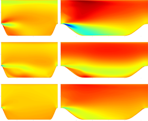
Analogous results are shown in figures 8 and 9 for the PH with  $\alpha =1.0$, which corresponds to a case of intermediate level of separation. Comparing the top and bottom rows of figures 8 and 9, we can see a remarkable similarity within the row and a significant change in the error propagation field from one row to the other. Turning implicit the linear term of the RANS has slightly diminished the maximum error, but the likeness between the error fields is impressive. The same can be said about the two strategies that included the optimised viscosity. The implicit treatment caused a timid effect that is difficult to identify. The mean velocity field information embedded in the eddy viscosity calculation of methods
  $EV_{DNS}\text{--}E$ and
  $EV_{DNS}\text{--}I$ leads to very low error levels, which are mainly concentrated near the flow detachment region for both mean velocity components. The top panels show the inability of the DNS RST to provide low error values. The red-like regions in figures 8(a) and 8(b) show positive errors concentrated in the recirculating zone. The negative errors of the blue-like region seem to correspond to an advection of errors near the detachment point. Figures 9(a) and 9(b) exhibit a red blob near the frontier of the recirculating zone at the lower part of the PH. The results shown here obeyed the same tendency in all the other configurations of the PH geometry of the database of Xiao et al. (Reference Xiao, Wu, Laizet and Duan2020), as shown in the supplementary data.

Figure 8. Error of the velocity component  $U_x$ in the PH for the configuration where
  $\alpha =1.0$: (a)
  $RST\text{--}E$; (b)
  $EV_{RST}\text{--}I$; (c)
  $EV_{DNS}\text{--}E$; (d)
  $EV_{DNS}\text{--}I$.

Figure 9. Error of the velocity component  $U_y$ in the PH for the configuration where
  $\alpha =1.0$: (a)
  $RST\text{--}E$; (b)
  $EV_{RST}\text{--}I$; (c)
  $EV_{DNS}\text{--}E$; (d)
  $EV_{DNS}\text{--}I$.
5.2. Performance of the new hybrid method
In this subsection, we compare three improved methods conceived to circumvent the high error propagation of the use of the DNS Reynolds stress data ( $RST\text{--}E$) and provide more accurate mean velocity fields. The first one,
  $EV_{DNS}\text{--}I$, is based on the works of Wu et al. (Reference Wu, Xiao and Paterson2018, Reference Wu, Xiao, Sun and Wang2019) and was already analysed in the last subsection. The second one is based on the RFV presented by Cruz et al. (Reference Cruz, Thompson, Sampaio and Bacchi2019), referred to as
  $RFV\text{--}E$. The third, is a new method proposed in the present work,
  $RFV$–
 $EV_{DNS}\text{--}I$ that combines aspects of the two previous ones, as described in § 4. These approaches provide quantities that can be used as targets for the application of ML techniques for the prediction of turbulent flows with low error propagation, as demonstrated by Wu et al. (Reference Wu, Xiao and Paterson2018) and Cruz et al. (Reference Cruz, Thompson, Sampaio and Bacchi2019).
Figures 10 and 11 show the error propagation in the SD for  $U_x$ and
  $U_y$, respectively. The columns represent different values of the Reynolds number,
  $Re=2200$,
  $Re=2900$ and
  $Re=3500$, from left to right. The rows compare each method,
  $EV_{DNS}\text{--}I$ (a),
  $RFV\text{--}E$ (b) and
  $RFV$–
 $EV_{DNS}\text{--}I$ (c).

Figure 10. Comparison of the error propagation on  $U_x$ obtained by the methods
  $EV_{DNS}\text{--}I$ (a),
  $RFV\text{--}E$ (b) and
  $RFV$–
 $EV_{DNS}\text{--}I$ (c) in the SD for different values of the Reynolds number.

Figure 11. Comparison of the error propagation on  $U_y$ obtained by the methods
  $EV_{DNS}\text{--}I$ (a),
  $RFV\text{--}E$ (b) and
  $RFV$–
 $EV_{DNS}\text{--}I$ (c) in the SD for different values of the Reynolds number.
The contours shown in figure 10 reveal that the methods  $RFV\text{--}E$ and
  $RFV$–
 $EV_{DNS}\text{--}I$ are able to reduce the error in the
  $x$-component of the mean velocity field more significantly than the method
  $EV_{DNS}\text{--}I$, which presented more concentrated errors near the bottom-left corner of the SD. The reason for this difference seems to be related to the fact that, in the case of
  $EV_{DNS}\text{--}I$, the information from the DNS mean velocity is injected into the linear part of the RST only while, in the RFV approaches, this DNS information is introduced to the divergence of the linear and nonlinear parts of the RST. We can notice that the approach
  $RFV\text{--}E$ has non-negligible errors near the symmetry lines of the boundary, top and right frontiers that are absent in the
  $EV_{DNS}\text{--}I$ and
  $RFV$–
 $EV_{DNS}\text{--}I$ results. Concerning the error propagation in
  $U_y$, shown in figure 11, we can also observe that the methods
  $RFV\text{--}E$ and
  $RFV$–
 $EV_{DNS}\text{--}I$ could attenuate more effectively the errors near the secondary recirculation flow. Again, the connection with error associated with the nonlinear part of the RST can explain the difference, since the nonlinear part is more responsible for the presence of the secondary flow. In this component, the three approaches presented non-negligible errors in the right symmetry line for all the
  $Re$ investigated. It is worth noticing that the symmetry filters applied to the SD database decreased the overall error in the domain, since comparing each of the four quadrants we could find quite non-symmetric fields. However, they were not effective in diminishing the localised errors close to the symmetry boundaries. This fact is probably responsible for the residual numerical errors in these boundaries, but it does not affect the main analysis.
The analogous results for the PH geometry are shown in figures 12 and 13 for two configurations, one associated with  $\alpha =0.5$ (left column), the most severe separation case, and another where
  $\alpha =1.5$ (right column) with a mild separation (see figure 5). Concerning the
  $U_x$ error propagation, figure 12, we can notice that the one associated with the
  $\alpha =1.5$ configuration is higher than the
  $\alpha =0.5$ one and that errors near the detachment point are advected by the flow. Since we adopted the simple difference in mean velocity, we can see that there are positive and negative errors. The case of
  $\alpha =1.5$,
  $EV_{DNS}\text{--}I$ presented the lowest negative and the highest positive error propagation value. In the
  $\alpha =0.5$ configuration, the advantage of the
  $RFV\text{--}E$ method over the
  $EV_{DNS}\text{--}I$ one is less pronounced, having a clear place near the detachment point where the errors are higher. The better accuracy of the
  $RFV$–
 $EV_{DNS}\text{--}I$ approach for
  $U_x$ is clear. In the case of
  $U_y$, figure 13, the error propagation is concentrated near the detachment and the reattachment points and the methods
  $EV_{DNS}\text{--}I$,
  $RFV\text{--}E$ and
  $RFV$–
 $EV_{DNS}\text{--}I$ exhibited a decreasing error propagation from left to right.

Figure 12. Comparison of the error propagation on  $U_x$ obtained by the methods
  $EV_{DNS}\text{--}I$ (a),
  $RFV\text{--}E$ (b) and
  $RFV$–
 $EV_{DNS}\text{--}I$ (c) in the PH for two values of the configuration parameter,
  $\alpha =0.5$ and
  $\alpha =1.5$.

Figure 13. Comparison of the error propagation on  $U_y$ obtained by the methods
  $EV_{DNS}\text{--}I$ (a),
  $RFV\text{--}E$ (b) and
  $RFV$–
 $EV_{DNS}\text{--}I$ (c) in the PH for two values of the configuration parameter,
  $\alpha =0.5$ and
  $\alpha =1.5$.
There is a concern with respect to the sign of  $\nu _{t\theta }$ when computed from (4.4) that affects the methods
  $EV_{DNS}\text{--}I$ and
  $RFV$–
 $EV_{DNS}\text{--}I$. To constrain the first-order term as a non-negative quantity is a safe procedure and in turbulent models we can impose this constraint in a straightforward manner. However, when one computes the coefficient of the projection of the RST provided by the DNS onto the mean rate-of-strain tensor provided by the DNS, the result can lead to negative values. In this case, we chose here not to split the RST into linear and nonlinear parts, which is equivalent of enforcing
  $\nu _{t\theta }=0$. We have tested the absolute value of
  $\nu _{t\theta }$ and we did not observe any significant change, probably because this has happened in few locations of the domain.
5.3. Relative error measures
There are some difficulties in proposing a single metric to evaluate relative errors. We show here some measures for the reader to have an indication of the gain in accuracy from one method to the other.
For the SD at  $Re=3500$, the
  $U_x$ component of the
  $EV_{DNS}\text{--}I$ method presented a maximum relative error of
  ${\rm \Delta} U_i^{max}=\max [\| \delta U_i\| / \|U_{i,{\theta }}\|]=6\,\%$, dropping to
  $0.6\,\%$ when using the proposed methodology (
 $RFV$–
 $EV_{DNS}\text{--}I$). In the
  $U_y$ component, this error measure was adapted, replacing
  $U_{i,{\theta }}$ by
  $\bar {U}_{i,{\theta }}$, due to the very small values in a large portion of the domain, leading to extremely high errors that do not represent the actual discrepancy. The
  $RST\text{--}E$ method presented an error of
  ${\rm \Delta} U_i^{max}=\max [\| \delta U_i\| / \|\bar {U}_{i,{\theta }}\|]=16\,\%$, while in the
  $EV_{DNS}\text{--}I$ method, the relative error dropped to 9 %, and exhibited the even smaller value of 4.3 % for the hybrid method (
 $RFV$–
 $EV_{DNS}\text{--}I$).
In the PH, instead of using the relative measure with respect to the mean, it is more conventional to use a normalisation with respect to the bulk velocity at the inlet ( $U_b$). With respect to figures 12 and 13, for the
  $\alpha =0.5$ configuration, the
  $U_x$ component of the
  $EV_{DNS}\text{--}I$ method presented a maximum error of 23 %, dropping to 21 % in the proposed approach,
  $RFV$–
 $EV_{DNS}\text{--}I$. In the
  $U_y$ component, the error dropped from 13 % using the
  $EV_{DNS}\text{--}I$ to 8 % in the hybrid method. For the
  $\alpha =1.5$ configuration, the
  $U_x$ component dropped from 35 % to 17 % in the same comparison (
 $EV_{DNS}\text{--}I$ and
  $RFV$–
 $EV_{DNS}\text{--}I$, respectively). In the
  $U_y$ component, the error decrease from one method to the other was from 16 % to 6 %.
6. Final remarks
We developed a series of methods to study the conditioning of the RANS equations and to test a new procedure to reduce the error with respect to the mean velocity field obtained from the solution of these equations.
Our conditioning analysis for the plane channel flow provided an explanation for the dependence with respect to the Reynolds number when we matched the conditions of the error analysis conducted by Thompson et al. (Reference Thompson, Sampaio, Alves, Thais and Mompean2016), i.e. by keeping the original non-uniformity and number of points of the DNS mesh, and by changing the linear operator from the one associated with a second-order derivative to the one associated with a first-order derivative.
The results of the SD and the PH revealed that the RANS equations are ill conditioned indeed. This means that, given a RST field near the correct Reynolds stress tensor field, the mean velocity field obtained from the solution of the RANS equations is far from the correct mean velocity field. In addition, turning implicit the linear part of the RST does not improve conditioning significantly. The procedures that lead to low error propagations were the ones where the DNS mean velocity field was introduced to compute the quantity to be modelled, with this quantity being the RST or the RFV.
We proposed a new ‘hybrid’ method, called here  $RFV$–
 $EV_{DNS}\text{--}I$, that combines the advantages reported by Wu et al. (Reference Wu, Xiao and Paterson2018), Wu et al. (Reference Wu, Xiao, Sun and Wang2019) and Cruz et al. (Reference Cruz, Thompson, Sampaio and Bacchi2019). It is a RFV approach that has an implicit term with the optimised eddy viscosity as a strong fixed quantity together with a more accurate representation of the nonlinear part of the RST by the injection of the mean velocity field information into the divergence of this quantity.
The conclusions stated above are supported by the more than ten simulations where the Reynolds number (in the SD) and the configuration (in the PH) were varied (see the supplementary data).
It is important to notice that increasing the Reynolds number will worsen the conditioning of the system. Therefore, for higher values of  $Re$, the difference between a procedure that uses information from the mean velocity field data and another that uses information of Reynolds stress tensor solely would be even higher. The statistics of higher
  $Re$ simulations need higher time averages to converge. For the plane channel, even for the highest Reynolds number case,
  $Re_\tau =5200$, we were able to recover the mean velocity profile with high accuracy by using the Reynolds stress shear component computed indirectly. This result indicates that the explicit procedure is already capable of reproducing the expected result. This fact and the decoupled results obtained with the SD and the PH corroborate the idea that our conclusions are extensible for high Reynolds numbers.
The implicit treatment was not able to induce a significant change in the accuracy of the solution, corroborating the common understanding in traditional CFD practice. However, we would like to point out that the implicit solver versions were more robust than their explicit counterparts. The implicit treatment leads to an increase in the convergence rate and the necessity of smoother values of under-relaxation parameters, which decreased substantially the computational costs. In addition, we would like to report that, in the PH geometry, it was challenging to build a set-up able to converge the explicit approaches. Therefore, the implicit treatment is highly recommended since in more complex geometries it is likely that this kind of approach would be decisive for convergence achievement.
Our analysis highlights some advantages of dealing with the Reynolds force vector, instead of the RST. In this regard, ideas like the ones developed by Perot (Reference Perot1999) can be useful for modelling purposes. In addition, the hybrid method proposed here brings other possible targets for ML, such as the divergence of the nonlinear part of the RST. As in the case of the RST, this strategy is constrained by invariance in the learning process, needing larger databases in order to enforce this constraint from data. From the perspective of data-driven modelling, aiming for a vector field as a target can also be an advantage when compared to a tensor field, since fewer components need to be learned.
Supplementary data
Supplementary data are available at https://doi.org/10.1017/jfm.2021.148.
Funding
We would like to thank Conselho Nacional de Pesquisa e Desenvolvimento (CNPq) Grant 304095/2018-4 and Coordenação de Aperfeiçoamento de Pessoal de Nível Superior (CAPES) Grant PROEX 803/2018 for financial support.
Declaration of interest
The authors report no conflict of interest.
Appendix A. Conditioning analysis of the plane channel flow
A.1. Explicit first-order system of equations
The first-order equation in plus units is given by
 \begin{gather} \frac{\textrm{d} U^{+}}{{\textrm{d} y}^{+}}=1-\frac{y^{+}}{R e_{\tau}}-R_{y x}^{+}, \end{gather}
 \begin{gather}\frac{\textrm{d} (U^{+}+\delta U)}{{\textrm{d} y}^{+}}=1-\frac{y^{+}}{R e_{\tau}}-(R_{y x}^{+}+\delta R). \end{gather}
Subtracting (A1) from (A2), we have that
 \begin{equation} -\frac{\textrm{d} (\delta U)}{{\textrm{d} y}^{+}}=\delta R.\end{equation}
Linearising the differential operator as a matrix,
 \begin{equation} \mathsf{A}_1(\delta \boldsymbol{U})=\delta \boldsymbol{R}^+_{yx}\Rightarrow \delta \boldsymbol{U}=\mathsf{A}^{{-}1}_1(\delta \boldsymbol{R}^+_{yx}).\end{equation}
 Hence, taking the norm of both sides of (A4), dividing this equation by  $\|\boldsymbol {U}^+\|$ and multiplying its right side by
  $\| \boldsymbol{R}^+_{yx}\|/\| \boldsymbol{R}^+_{yx}\|$, gives
 \begin{equation} \frac{\|\delta \boldsymbol{U}^+\|}{\|\boldsymbol{U}^+\|}<\frac{ \|\mathsf{A}_1^{{-}1} \| \|\boldsymbol{R}_{yx}^{+}\|}{\| \boldsymbol{U}^+\|} \frac{ \|( \delta \boldsymbol{R}_{yx}^{+}) \| }{\|\boldsymbol{R}_{yx}^{+}\|}.\end{equation}
A.2. Implicit case
As seen in the last section, when the RST is treated implicitly, the momentum equation for the plane channel takes the form given by
 \begin{equation} (1+{\tilde{\nu}}_t^{*})\frac{\textrm{d} {U}^{+}}{{\textrm{d} y}^{+}}=1-\frac{y^{+}}{R e_{\tau}}.\end{equation}
 When the RST is perturbed, it generates an error in  ${\tilde {\nu }}_t^{*}$ and, consequently, in the mean velocity field. Since
  ${[R^+_{yx}]_{\theta }}$ is a perturbed Reynolds stress component, the perturbed
  $\nu ^{*}_t$ is given by
 \begin{equation} \nu_t^{*}=\frac{[R^+_{yx}]_{\theta}}{{\rm d}U^+_{\theta}/{\textrm{d} y}^+}. \end{equation}
Then, (A6) is given by
 \begin{equation} {(1+\nu_t^{*})\frac{\textrm{d} ({U^+_{\theta}}+\delta U)}{{\textrm{d} y}^{+}}=1-\frac{y^{+}}{R e_{\tau}}}.\end{equation}
Subtracting the original equation from (A8),
 \begin{equation} {-\frac{\textrm{d} (\delta U^{+})}{{\textrm{d} y}^{+}}=\frac{1}{1+\nu_t^{*}}\delta {R}_{yx}^{+}}. \end{equation}
 Linearising the differential operator related to  $\delta U$,
 \begin{equation} {\delta \boldsymbol{U}^+{=} \frac{1}{1+\nu_t^{*}} \mathsf{A}_1^{{-}1}(\delta \boldsymbol{R}_{yx}^{+})= [(1+\nu_t^{*}) \mathsf{A}_1]^{{-}1}(\delta \boldsymbol{R}_{yx}^{+}).}\end{equation}
Where we can notice that the operator  $\mathsf{A}_1$ has changed to
  ${(1+\nu _t^{*} ) \mathsf{A}_1}$ in the implicit treatment. Writing the relative error in the output as a function of the relative input error, one arrives at
 \begin{equation} {\frac{\|\delta \boldsymbol{U}^+\|}{\|\boldsymbol{U}^+\|}<\frac{ \|[(1+\tilde{\nu}_t^{*}+\delta \nu_t^{*})\mathsf{A}_1]^{{-}1} \|\|\boldsymbol{R}_{yx}^{+}\|}{\| \boldsymbol{U}^+\|} \frac{ \|( \delta \boldsymbol{R}_{yx}^{+}) \| }{\|\boldsymbol{R}_{yx}^{+}\|},}\end{equation}
where  $\delta \nu _t^{*}$ is the perturbation in the eddy viscosity. We can notice that part of the error is now inside the linear operator itself due to an implicit treatment of RST. Therefore, this fact brings a warning since the unperturbed matrix is recommended for use to assess the conditioning. Otherwise, the size of the error will have an influence on the conditioning analysis. Strang (Reference Strang2006) and Meyer (Reference Meyer2000) call attention to this point, when a matrix perturbation analysis is made. In this case, after some manipulation, we get the following expression:
 \begin{equation} \frac{\|\delta \boldsymbol{U}^+\|}{\|\boldsymbol{U}^+{+}\delta \boldsymbol{U}^+\|} < \|[(1+{\tilde{\nu}}_t^{*})\mathsf{A}_1]^{{-}1} \|(1+{\tilde{\nu}}_t^{*})\mathsf{A}_1\| \frac{\|[\delta \nu_t^{*}\mathsf{A}_1]\|}{\|(1+{\tilde{\nu}}_t^{*})\mathsf{A}_1\|}. \end{equation}
This shows that, considering a perturbation in the linear operator leads to a relative error where the norm of the original velocity vector is embedded with the error propagation. In cases where the error propagation is not low, this term cannot be neglected such as, for example, the high  $Re_{\tau }$ cases of the plane channel. We would like to point out that computing the conditioning number with respect to the linear operators
  $(1+\nu _t^{*})\mathsf{A}_1$ or
  $(1+\tilde {\nu }_t^{*})\mathsf{A}_1$ made no significant difference.
A.3. Parallel between solving the linear system of equations and integrating the local error
An additional insight into the reason why the errors of the  $Re_{\tau }=5200$ case are higher, even when the conditioning number associated with the linear system is lower than other cases, comes from evaluating the structure of this linear system from a local point of view, inspired by the analysis of Wu et al. (Reference Wu, Xiao, Sun and Wang2019). In this case,
  $\mathsf{A}_1(\delta \boldsymbol {U}^+)=\delta \boldsymbol{R}^+_{yx}$ written in a matrix form considering a uniform mesh and central differences as
 \begin{equation} \frac{2}{{\rm \Delta} y^+}\left[ \begin{array}{@{}cccccc@{}} \mathcal{B}_1 & \mathcal{C}_1 & & & & \\ 1 & 0 & -1 & & & \\ & 1 & 0 & -1 & & \\ & & \ddots & \ddots & \ddots & \\ & & & 1 & 0 & -1 \\ & & & & \mathcal{A}_n & \mathcal{B}_n \end{array} \right] \left[ \begin{array}{@{}c@{}} \delta U^+_1\\ \delta U^+_2\\ \delta U^+_3\\ \vdots\\ \delta U^+_{n-1}\\ \delta U^+_n \end{array} \right]= \left[ \begin{array}{@{}c@{}} \delta R^+_{yx} (1)\\ \delta R^+_{yx} (2)\\ \delta R^+_{yx} (3)\\ \vdots\\ \delta R^+_{yx} (n-1)\\ \delta R^+_{yx} (n) \end{array} \right], \end{equation}
where the first and last lines are related to the boundary conditions. The  $i$th line of the system (
 $i\neq 1$ and
  $i\neq n$) is written as
 \begin{equation} \delta U_{i-1}-\delta U_{i+1}=0.5{\rm \Delta} y^+\delta R^+_{yx} (i).\end{equation}
Applying the  $\sum ^i_{i'=1}$ operator to (A14) we get
 \begin{equation} \delta U_{i+1}+\delta U_{i}=\delta U_{1}+\delta U_{2}-0.5{\rm \Delta} y^+{-}\sum^i_{i'=1}\delta R^+_{yx} (i').\end{equation}
Hence, we notice the relation between the current analysis and the integral obtained in (2.4). The errors  $\delta \boldsymbol{R}^+_{yx}$ of each position are accumulated in the error propagation. From the boundary conditions, it is expected that
  $\delta U_{1}=0$, since
  $U_1=0$ without uncertainty. Thus, for a uniform error in the whole domain,
  $\delta R^+_{yx}(i)=-0.5 {\rm \Delta} y^+ {\rm \Delta} \varepsilon$ for example,
 \begin{equation} \delta U_{n}+\delta U_{n-1}\approx (n-2){\rm \Delta} \varepsilon,\end{equation}
and the boundary condition in  $n$ determines
  $\delta U_{n}$ and
  $\delta U_{n-1}$. Therefore, we observe that, in the case where the perturbation is the same at any position, the error propagation is more severe farther from the wall. This result is consistent with the output of the analysis conducted by Thompson et al. (Reference Thompson, Sampaio, Alves, Thais and Mompean2016) and with the behaviour of the local conditioning number provided by Wu et al. (Reference Wu, Xiao, Sun and Wang2019), where we can notice that local conditioning number increases with the wall distance. Since the number of points employed in the Lee & Moser (Reference Lee and Moser2015) DNS database is much higher for the
  $Re_{\tau }=5200$ case, it is the error propagation to the velocity profile. The generalisation to a non-uniform mesh is straightforward. This rationale also applies to the second-order derivative operator, since the structure of the corresponding matrix is such that a uniform injected error has a higher impact on positions farther from the wall in the same fashion as the first derivative.
Appendix B. An alternative form of computing the optimised turbulent viscosity
The optimised turbulent viscosity employed here and by Wu et al. (Reference Wu, Xiao and Paterson2018) was obtained from a projection of the Reynolds stress tensor onto the space generated by  ${\boldsymbol{\mathsf{S}}}$ (Thompson et al. Reference Thompson, Mompean and Thais2010). An alternative procedure would be to compute
  $\nu _{t\theta }$ from a projection of the RFV onto the space of the
  $\boldsymbol {\nabla }\boldsymbol {\cdot } {\boldsymbol{\mathsf{S}}}$ as developed next. We notice that
  $2\boldsymbol {\nabla }\boldsymbol {\cdot } {\boldsymbol{\mathsf{S}}}=\nabla ^2{\boldsymbol v}$ in incompressible flows.
We begin by splitting the RST into a linear part with respect to  ${\boldsymbol{\mathsf{S}}}$ and a nonlinear one,
  ${\boldsymbol{\mathsf{R}}}^{nl}$, and apply the divergence operator on this equation, as
 \begin{equation} {\boldsymbol{\mathsf{R}}}=2\nu_t{\boldsymbol{\mathsf{S}}}+{\boldsymbol{\mathsf{R}}}^{nl}\Rightarrow \boldsymbol{\nabla}\boldsymbol{\cdot} {\boldsymbol{\mathsf{R}}}=\nu_t\nabla^2{\boldsymbol v}+2{\boldsymbol{\mathsf{S}}}\boldsymbol{\cdot} \boldsymbol{\nabla}\nu_t+\boldsymbol{\nabla}\boldsymbol{\cdot} {\boldsymbol{\mathsf{R}}}^{nl}. \end{equation}
Applying the scalar product of (B1) with respect to  $\nabla ^2{\boldsymbol v}$ we find
 \begin{equation} (\boldsymbol{\nabla}\boldsymbol{\cdot} {\boldsymbol{\mathsf{R}}})\boldsymbol{\cdot} \nabla^2{\boldsymbol v}= \nu_t\nabla^2{\boldsymbol v}\boldsymbol{\cdot} \nabla^2{\boldsymbol v}+[2{\boldsymbol{\mathsf{S}}}\boldsymbol{\cdot} \boldsymbol{\nabla}\nu_t+\boldsymbol{\nabla}\boldsymbol{\cdot} {\boldsymbol{\mathsf{R}}}^{nl}]\boldsymbol{\cdot} \nabla^2{\boldsymbol v}.\end{equation}
Then, we define the quantity  $\nu _t$ by imposing that the vector
  $2{\boldsymbol{\mathsf{S}}}\boldsymbol {\cdot } \boldsymbol {\nabla }\nu _t+\boldsymbol {\nabla }\boldsymbol {\cdot } {\boldsymbol{\mathsf{R}}}^{nl}$ is orthogonal to the Laplacian of
  ${\boldsymbol v}$. Since the last term vanishes, the eddy viscosity is given by
 \begin{equation} \nu_t=\frac{(\boldsymbol{\nabla}\boldsymbol{\cdot} {\boldsymbol{\mathsf{R}}}) \boldsymbol{\cdot} \nabla^2{\boldsymbol v}}{\nabla^2{\boldsymbol v}\boldsymbol{\cdot} \nabla^2{\boldsymbol v}}.\end{equation}
Once  $\nu _t$ is defined, we can incorporate this quantity into the implicit linear term when representing the RFV as
 \begin{equation} \boldsymbol{\nabla}\boldsymbol{\cdot} {\boldsymbol{\mathsf{R}}}= \boldsymbol{\nabla}\boldsymbol{\cdot} (2\nu_t{\boldsymbol{\mathsf{S}}}) +\boldsymbol{\nabla}\boldsymbol{\cdot} {\boldsymbol{\mathsf{R}}}^{nl},\end{equation}
where the RFV,  ${\boldsymbol r}=\boldsymbol {\nabla }\boldsymbol {\cdot } {\boldsymbol{\mathsf{R}}}$, is decoupled into the Boussinesq vector
  ${\boldsymbol r}_b\equiv \boldsymbol {\nabla }\boldsymbol {\cdot } (2\nu _t{\boldsymbol{\mathsf{S}}})$ and the nonlinear Reynolds force vector,
  ${\boldsymbol r}^{nl}\equiv \boldsymbol {\nabla }\boldsymbol {\cdot } {\boldsymbol{\mathsf{R}}}^{nl}$. We notice that (B3) can be computed using full information from the mean velocity field, since
  ${\boldsymbol r}$ can be computed indirectly not using
  ${\boldsymbol {\nabla }\boldsymbol {\cdot } {\boldsymbol{\mathsf{R}}}_{\theta }}$ (Cruz et al. Reference Cruz, Thompson, Sampaio and Bacchi2019) and, needless to say,
  $\nabla ^2{\boldsymbol v}$ comes directly from the mean velocity field of the DNS database. Therefore, linear and nonlinear parts of the RFV can be computed with no use of the
  ${\boldsymbol{\mathsf{R}}}_{\theta }$, the RST provided by the DNS database, in contrast to (4.6), where
  ${\boldsymbol{\mathsf{R}}}_{\theta }$ is employed.
We came to this new form of computing  $\nu _t$ after we had obtained all the results of the present investigation. Preliminary simulations with this new form indicate a promising path that was not possible to explore for this work, but we intend to do so in the near future.


