


1. Introduction
Collision and subsequent coalescence of drops or aggregation of particles influences the evolution of many commonly encountered systems. The non-continuum hydrodynamics and coupling of differential sedimentation with turbulence, which are expected to play an important role in driving collisions between particles of 5 to 50  $\mathrm {\mu }$m radii in a gas, will be studied in detail. We treat turbulence experienced by colliding particles as a persistent uniaxial compressional flow in line with the model by Saffman & Turner (Reference Saffman and Turner1956) which forms the basis of their well-known prediction for the ideal collision rate of non-sedimenting drops in isotropic turbulence. Particles much smaller than the Kolmogorov scale, which is
  $O$(1 mm) in many applications such as droplets in clouds and aerosol reactors, experience turbulence as a local linear flow consisting of superimposed straining and rotational motions with the former being most effective in driving collisions. The distribution of straining flows in turbulence is skewed toward motions resembling uniaxial compressional motion (see Ashurst et al. Reference Ashurst, Kerstein, Kerr and Gibson1987). While the strain rate in turbulence only persists for a strain of approximately
  $2.3$ (see Yeung & Pope Reference Yeung and Pope1989) Brunk, Koch & Lion (Reference Brunk, Koch and Lion1998) found only approximately a 20 % change of the ideal collision rate when accounting for the finite correlation time of the strain rate.
The frozen flow field treatment of turbulence is applicable to a wide range of aerosol collision problems. The aggregational growth of carbon black, pigments and other commercially valuable materials occurs in the turbulent gas flow of an aerosol reactor (see Buesser & Pratsinis Reference Buesser and Pratsinis2012). Thus coupling of the velocities induced by turbulence with differential sedimentation and shaped by non-continuum hydrodynamics will be crucial in determining the collision rate. The results of this study could provide a better understanding of the design of flow conditions to produce a desired degree of aggregation. In clouds the evolution of droplets in the size gap, of 15 to 40  $\mathrm {\mu }$m radius, is not fully understood. At this bottleneck condensation and coalescence driven by differential sedimentation are both slow processes. For drops in this size range, turbulence driven motion is expected to augment differential sedimentation to enhance the coalescence rate while non-continuum hydrodynamics will play a major role in shaping it.
Collision of spheres settling in a local linear flow may arise in many non-turbulent systems. In systems designed to remove particles such as porous aerosol filters (see Jaworek et al. Reference Jaworek, Sobczyk, Krupa, Marchewicz, Czech and Śliwiński2018) and impactors (see Malá et al. Reference Malá, Rulík, Bečková, Mihalík and Slezáková2013) interparticle collisions driven by gravity and the local linear flow may affect the particle size distribution in non-dilute aerosols. The efficiency of atomization of drops in applications such as engines can be impeded by coalescence (see Laurent & Massot Reference Laurent and Massot2001) driven by deceleration of the spray, experienced by droplets of different size as a differential body force, and a local uniaxial compressional flow in the jet.
Hydrodynamic interactions play an important role in interparticle collisions in a gas or liquid. Continuum hydrodynamic lubrication forces do not allow collisions to occur in finite time. Thus, other interparticle interactions become crucial to obtain a non-zero collision rate. In a gas, collision can occur due to the breakdown of the continuum (Sundararajakumar & Koch Reference Sundararajakumar and Koch1996; Chun & Koch Reference Chun and Koch2005). We will see that for drop sizes where straining flow and sedimentation typically compete, non-continuum lubrication gas flow is more important than other considerations that may lead to collision including van der Waals attractions, mobility of the interface of the water droplets with air and compressibility of the gas. Thus, we will evaluate the collision rate of particles driven by the coupled action of gravity and uniaxial compressional flow in the presence of a non-continuum gas. Additionally, since deformation of the droplets is not expected to be important we will treat them as hard spheres.
One of the earliest studies on coalescence was carried out by Smoluchowski (Reference Smoluchowski1918) who found the ideal collision rate for two non-interacting spheres, with species  $i$ of radius
  $a_i$ and number density
  $n_i$, settling in a quiescent fluid with a relative velocity of
  $V_{rel}$ to be
  $n_1n_2 {\rm \pi}[a_1+a_2]^2 V_{rel}$. Zeichner & Schowalter (Reference Zeichner and Schowalter1977) determined the collision rate of non-interacting spheres in a frozen uniaxial compressional flow to be
  $[4{\rm \pi} /(3\sqrt {3})]n_1n_2 \dot {\gamma } [a_1+a_2]^3$, where
  $\dot {\gamma }$ is the compression rate. The coupled system of spheres settling in linear flow has not been analysed and will be the focus of this study. Literature exists that studies the uncoupled problems of particle motion due the linear flow (see Curtis & Hocking Reference Curtis and Hocking1970; Wang, Zinchenko & Davis Reference Wang, Zinchenko and Davis1994) or sedimentation (see Davis Reference Davis1984) and includes continuum hydrodynamic interactions and colloidal forces with focus typically on van der Waals attractions. These collision studies are pertinent to particle motion in liquids where the van der Waals force is the predominant mechanism to overcome lubrication forces and enable surface-to-surface contact. In contrast, particle collision in a gas usually results from the non-continuum behaviour of the medium (see Sundararajakumar & Koch Reference Sundararajakumar and Koch1996; Chun & Koch Reference Chun and Koch2005), but this case has not been extensively studied. For sedimenting spheres (Davis Reference Davis1984) used a Maxwell slip approximation. This is only an accurate description of non-continuum behaviour at separations much larger than the mean free path of the gas. However, during a collision, particle pairs will pass through all possible separation gaps including those comparable to and smaller than the mean free path. The non-continuum behaviour valid at all separations was calculated by Sundararajakumar & Koch (Reference Sundararajakumar and Koch1996) and used by Chun & Koch (Reference Chun and Koch2005) for a monodisperse suspension coagulating due to isotropic turbulence. There is no comparable study for a polydisperse system, frozen linear flow or differential sedimentation. In our study, we will analyse the collision rate for polydisperse spheres settling in a linear flow while interacting through non-continuum hydrodynamic interactions.
The collision dynamics and rate can be influenced by the inertia of the particles or drops, which is much larger than the inertia of the gas. An estimate of the particle inertia is the Stokes number  $St_i=\tau _{p,i}/\tau _f$, where the particle response time of species
  $i$ is
  $\tau _{p,i}=2\rho (a_i)^2/(9\mu )$,
  $\mu =\rho _f \nu$ is the dynamic viscosity of the gas,
  $\nu$ its kinematic viscosity,
  $\rho$ is the particle density,
  $\rho _f$ is the fluid density,
  $g$ acceleration due to gravity and the flow time scale is
  $\tau _f$.
The turbulent dissipation rate  $\epsilon$ is typically of the order of
  $0.01\ \textrm {m}^2\ \textrm {s}^{-3}$ in a cloud, leading to a time scale for turbulent shear flow of
  $\tau _f=(\nu /\epsilon )^{1/2}=3.9 \times 10^{-2}$ s. The Stokes number based on turbulent shear then ranges from 0.07 to 0.5 across the size gap
  $a_i=15$ to 40
  $\mathrm {\mu }$m. Although these values are not asymptotically small, the first effect of particle inertia at modest Stokes number is to enhance the local pair probability without changing the local collisional dynamics (Sundaram & Collins Reference Sundaram and Collins1997). This enhancement has been extensively studied (Ireland, Bragg & Collins Reference Ireland, Bragg and Collins2016a,Reference Ireland, Bragg and Collinsb; Dhariwal & Bragg Reference Dhariwal and Bragg2018). At small Stokes numbers the collision rate can be estimated as the product of the enhanced pair probability due to inertial clustering and a rate for local inertia-less coalescence (Chun & Koch Reference Chun and Koch2005). In aerosol reactors
  $\epsilon$ is higher leading to smaller values of
  $\tau _f$, but the smaller particle sizes compensate leading to similar estimates of
  $St$.
$St$.
For differential sedimentation  $\tau _f=(a_1+a_2)/V_{rel}$ where the relative velocity is
  $V_{rel}=2\rho ((a_2)^2-(a_1)^2)g/9\mu$. The Stokes number based on differential sedimentation for drops in the size gap (15 to 40
  $\mathrm {\mu }$m) ranges from
  $5(1-\kappa )$ to
  $96(1-\kappa )$ and can be quite large for drops with substantially different radii
  $1-\kappa =\textit {O}(1)$. Here, the particle size ratio
  $\kappa = a_2/a_1$. However, condensation drives a population of droplets toward monodisperse size distributions and for drops with
  $1-\kappa =\textit {O}(10^{-2})$, for which turbulent shear and differential sedimentation compete to control the collision dynamics, the Stokes number for each driving force is less than one. In the present study we will calculate the collision rate for inertia-less local collisions recognizing that this calculation will be most accurate for small drops but may also set a reference rate to be compared with future analyses that include particle inertia.
In aerosol reactors, an important component of the collision dynamics is the Brownian motion. However, its effect becomes weak at larger sizes and for the largest particles, with radii of approximately  $1\ \mathrm {\mu }$m, acceleration-induced body forces can potentially be significant. Because of the small particle response times of these particles, the acceleration due to the mean gas flow is larger than that due to the relative motion of the particles, making the present analysis applicable.
We consider a dilute system since particle volume fractions are typically small  $\textit {O}(10^{-6})$ in clouds (Grabowski & Wang Reference Grabowski and Wang2013), aerosol reactors (Balthasar et al. Reference Balthasar, Mauss, Knobel and Kraft2002) and separators. Thus, we consider pairwise interactions. The flux of two spheres coming into contact with each other sets the collision rate. This flux, in turn, is related to the number density of spheres, the relative velocity of the spheres and the particle pair trajectories resulting from this relative velocity. The relative velocity is given as the vector sum of contributions driven by uniaxial compression and differential sedimentation. These themselves, due to the inertia-less nature of the system, are expressed through a mobility formulation. These mobilities will capture the hydrodynamic, interparticle interactions.
For an ideal collision with no interparticle interactions, the relative velocity is solenoidal everywhere and the pair distribution function at contact equals the square of the number density in the bulk suspension. Thus, it is possible to evaluate, for a pure uniaxial compressional flow or pure sedimentation (uncoupled) problem, the collision rate in terms of an explicit analytical expression (see Smoluchowski Reference Smoluchowski1918; Zeichner & Schowalter Reference Zeichner and Schowalter1977). For the coupled problem, we obtain a closed form analytical result as a function of the strength of gravity relative to the linear flow for the special case in which the compressional axis is aligned with gravity. For the case of a distribution of compressional flows whose axes are isotropically distributed, we obtain a numerical result. These results capture the collision dynamics pertinent to vertically aligned compressional flows and persistent isotropic turbulent flows, respectively.
Including hydrodynamic interactions changes the pair distribution function and retards the relative velocity when the spheres approach each other, causing the collision rate to diminish relative to the ideal case. The collision efficiency, defined as the collision rate with interparticle interactions divided by the ideal collision rate, is used to quantify this effect. The collision efficiency cannot be expressed in a closed analytical form even for uncoupled driving forces. However, it is possible to express it in terms of an integral over radial positions of an integrand involving the mobilities, which capture interparticle interactions (see Batchelor & Green Reference Batchelor and Green1972; Batchelor Reference Batchelor1982; Davis Reference Davis1984; Wang et al. Reference Wang, Zinchenko and Davis1994). For coupled driving forces, even this is not possible and so trajectory analysis is used in our study. In this method a test sphere is fixed at the origin and its collision rate with a set of satellite spheres is evaluated. Satellite spheres leading to collision, i.e. possessing inward radial velocity during contact, are integrated backward in time until they reach large separations. At large separations the flux is easier to evaluate since the pair probability reverts to its bulk value and the relative velocity can be computed without interparticle interactions. As a result, the collision rate can be evaluated in terms of the collisional area through which particles destined for collision pass.
The mobility matrix for a pair of particles can be expressed in terms of a set of coefficients that depend only on the radial separation and capture the hydrodynamic interactions between the particles. Comprehensive results are available for the mobilities of unequal sized spheres with continuum Stokes flow interactions (see Jeffrey & Onishi Reference Jeffrey and Onishi1984; Jeffrey Reference Jeffrey1992; Kim & Karrila Reference Kim and Karrila2013). However, continuum lubrication does not allow contact to occur in a finite time and leads to a collision rate of zero. Sundararajakumar & Koch (Reference Sundararajakumar and Koch1996) showed that non-continuum hydrodynamic interactions allow collisions to occur in finite time. The importance of non-continuum interactions is quantified by the Knudsen number, defined as  $Kn=\lambda _0/a^*$, where
  $\lambda _0$ is the mean free path and
  $a^*=(a_1+a_2)/2$ is the mean of the sphere radii
  $a_1$ and
  $a_2$. We will use an expression for the non-continuum mobility that is valid when
  $Kn \ll 1$ for all interparticle separations
  $h^*$ including separations
  $h^*/a^* =O(Kn)$ that are comparable to the mean free path of the gas. Tangential mobilities are not expected to be strongly influenced by the breakdown of continuum, because the continuum flow tangential mobility remains finite at contact. Thus, continuum hydrodynamics will be used for the tangential motion at all separations.
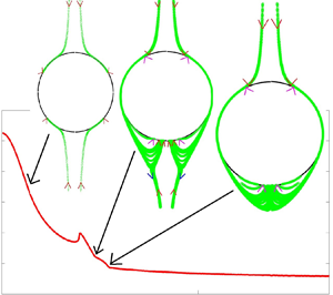
The collision rate with non-continuum hydrodynamic interactions depends on the Knudsen number, representing the strength of non-continuum effects, the orientation of the compressional axis relative to gravity and the relative strength of gravity and compressional flow as well as the particle size ratio  $\kappa =a_2 / a_1$. We will consider
  $\kappa =0.9$ and 0.5 to sample cases with nearly equal and widely separated radii, and will more thoroughly span the other parameters to capture important features of the collision dynamics. Particular attention will be given to the manner in which complex particle pair trajectories lead to non-trivial behaviour of the observed collision rate. A majority of the non-trivial behaviour is seen when the satellite and test sphere are close to each other. The hydrodynamic interactions cause the satellite sphere to be excluded from certain regions or open up new regions for the collision to occur. In a time-reversed motion, these complex trajectories include the satellite sphere either starting and ending on the test sphere or taking a circuitous path around the test sphere. Even at large separations from the test sphere the satellite sphere trajectories can change direction sharply due to the coupling of gravity with the uniaxial compressional flow. However, this class of complex trajectories does not directly affect the collision rate.
In the following sections, we will calculate the collision rate for an inertia-less dilute system of spheres settling in a uniaxial compressional flow. In § 2 we will set up the governing equations and present the relevant scales in the system. Then we will evaluate the ideal collision rate for coupled gravitational and straining driven motion in § 3. In § 4 we will obtain the uniformly valid radial and tangential mobilities. The former include non-continuum lubrication as well as a continuum description of hydrodynamic interactions outside the lubrication regime. The mobilities will be used in § 5 to evaluate the collision rate for a wide range of values of  $Kn$ and the strength and orientation of the uniaxial compressional flow with respect to gravity. In § 6 we will present results for the collision efficiency to describe the impact hydrodynamics has on the collision rate. We will also derive an expression for the collision efficiency in the pure linear flow as well as the purely gravity driven case. Finally in § 7 we will summarize the results of our study and discuss their implications.
2. Formulation
The collision rate  $K_{12}$ specifies the number of collisions per unit volume per time between spheres with radii
  $a_1$ and
  $a_2$ and number densities
  $n_1$ and
  $n_2$. For drops that coalesce on collision,
  $K_{12}$ can be used to determine the rate of change of the drop number density. For the simple case in which only two species are present the rate of change of the number density of one them is given as,
 \begin{equation} \frac{\textrm{d} n_1}{\textrm{d} t}=-K_{12}. \end{equation}
In more general circumstances, the rate constant  $C_{12}=K_{12}/(n_1 n_2)$ can be used in an integral equation for the drop size distribution. Due to the dilute nature of the suspension three or higher body interactions are highly unlikely and only the interaction and collision of two species is considered. The two-species rate
  $K_{ij}$ can be expressed as an integral of the flux of particle pairs over the collision area,
 \begin{equation} K_{12}= -n_1 n_2 \int_{(r'=a_1+a_2)\& (\boldsymbol{v}' \boldsymbol{\cdot} \boldsymbol{n}'<0)} (\boldsymbol{v}' \boldsymbol{\cdot} \boldsymbol{n}') P\,\textrm{d} A', \end{equation}
where  $\boldsymbol {v}'$ is the relative velocity,
  $r'$ is the radial separation between the centre of the two spheres,
  $P$ is the pair probability and captures the local species concentration relative to the bulk and
  $\boldsymbol {n}'$ represents the outward normal at the contact surface. The radial velocity is
  $\boldsymbol {v}' \boldsymbol{\cdot} \boldsymbol {n}'$.
To simplify the analysis, we scale the problem. The characteristic length is chosen to be  $a^*=(a_1+a_2)/2$. This sets the range of non-dimensional radial separations between the centres of the two spheres to be
  $r = 2$ (referred to as the collision sphere) to
  $\infty$ (where one sphere does not influence the other). The geometry of the two-species system is captured through
  $\kappa =a_1/a_2$ the relative size of the spheres, with
  $\kappa \in (0,1]$. Assuming negligible inertia, of both fluid and particles, allows scaling of the relative velocity with the characteristic velocity
  $\dot {\gamma } a^*$, the characteristic velocity in the frozen uniaxial compressional flow (the imposed linear flow), with
  $\dot {\gamma }$ being the strain rate along the axis of compression. The relative velocity due to gravity is captured through
  $Q=(2\rho g(a_2^2-a_1^2)/[9\mu ])/(\dot {\gamma } (a_1+a_2)/2)$, where
  $g$ is the acceleration due to gravity, and
  $\mu$ is the gas viscosity. A sketch of the two sphere system is shown in figure 1. The collision rate over the collision sphere, which scales as
  $n_1n_2\dot {\gamma } (a_1+a_2)^3$, can be expressed as,
 \begin{equation} \frac{K_{12}}{ n_1n_2\dot{\gamma} (a_1+a_2)^3}=-{\frac{1}{8}} \int_{(r=2)\& (\boldsymbol{v} \boldsymbol{\cdot} \boldsymbol{n}'<0)} (\boldsymbol{v} \boldsymbol{\cdot} \boldsymbol{n}') P\,\textrm{d} A. \end{equation}
The non-dimensional relative velocity  $\boldsymbol {v}$ in an extensional flow with strain rate tensor
  $\boldsymbol {E}$ and gravity directed along the negative Z-axis is given as,
 \begin{align} v_i &= E_{ij}r_j- \left[A\frac{r_i r_k}{r^2}+B \left(\delta_{ik}-\frac{ r_i r_k}{r^2}\right) \right]E_{kl}r_l \nonumber\\ &\quad - \left[L\frac{r_i r_k}{r^2}+M \left(\delta_{ik}-\frac{ r_i r_k}{r^2}\right) \right]Q\delta_{k3}. \end{align}
The mobility formulation is used because of the inertia-less nature of the system;  $A$ and
  $B$ correspond to the radial and tangential mobility in linear flow while
  $L$ and
  $M$ correspond to the radial and tangential mobility due to sedimentation. The uniaxial compressional flow has one of its extensional axes parallel to the
  $Y$ axis. The other extensional axis and the compressional axis lie in the
  $X$–
$X$– $Z$ plane. The angle between the compressional axis and gravity is
  $\alpha$. The rate of strain tensor is given as,
 \begin{equation} \boldsymbol{\mathsf{E}} = \frac{1}{4}\begin{bmatrix} 3\cos 2\alpha-1 & 0 & -3\sin 2\alpha \\ 0 & 2 & 0\\ -3\sin 2\alpha & 0 & -3\cos 2\alpha-1 \end{bmatrix}. \end{equation}
In spherical coordinates ( $r, \theta , \phi$) with the polar angle
  $\theta$ measured from the positive
  $Z$ axis and the azimuthal angle
  $\phi$ measured from the
  $X$ axis, the relative velocity is given as,
 \begin{align} v_r &= -LQ \cos \theta+ \frac{(A-1)r}{16} \{ 1 + 3 [\cos 2\theta+\cos 2\alpha (1+3\cos 2\theta) \nonumber\\ &\quad + 4\cos 2\phi \sin^2 \alpha \sin^2 \theta + 4\cos\phi\sin 2\alpha \sin 2\theta ] \} , \end{align}
 \begin{align} v_{\theta}&= \frac{3(B-1)r}{16}\left(4\cos2 \theta \cos \phi \sin 2 \alpha + \sin 2 \theta[2 \cos 2 \phi \sin^2 \alpha-1-3\cos \alpha] \right) \nonumber\\ &\quad + M Q \sin \theta, \end{align}
 \begin{equation} v_{\phi}= -\tfrac{3}{2}(B-1)r \sin \alpha \sin \phi \left(\cos \alpha \cos \theta + \cos \phi \sin \alpha \sin \theta \right) .\end{equation}
Figure 1. Sketch of the two spheres separated by  $\boldsymbol {r}$ and acted on by gravity and uniaxial compressional flow; ‘I’ is the test sphere of radius
  $a_1$ placed at the origin. It is approached by satellite sphere ‘II’ of radius
  $a_2$; ‘III’, referred to as the collision sphere, is the locus of the centre of sphere ‘II’ when it is in contact with sphere ‘I’. The axis of compression indicated by the dash-dot line is inclined at an angle of
  $\alpha$ relative to gravity.
When calculating the ideal collision rate, there is no interparticle interaction of any kind and so the mobilities will take the trivial values  $A=0,\ B=0,\ L=1,\ \textrm {and}\ M=1$. For the full collision calculation the mobilities will capture the hydrodynamic interaction. The uniformly valid mobilities will capture non-continuum lubrication and long range continuum hydrodynamics.
The continuum hydrodynamic interactions between rigid spheres, while relevant at large separations, do not fully account for the particle dynamics upon close approach. They yield a mobility for normal motion that decreases in proportion to the gap thickness, so that the gap cannot go to zero in finite time under the action of a finite compressive force. For finite time collision events other mechanisms must become important to describe the relative velocity at small separations between colliding drops. For particles colliding in air due to the coupled effects of gravity and shearing flows, we expect the breakdown of the continuum to be the predominant mechanism facilitating collision. To test this hypothesis, we compare the surface to surface separation at which non-continuum gas flow modifies the velocity substantially to the separation where other mechanisms such as van der Waals forces, interface mobility, gas compressibility and drop deformability become important. We will use  $h^*$ to denote the dimensional surface-to-surface separation. We will consider water droplets in air, thus assuming the drop-to-medium viscosity ratio to be about
  ${\hat {\mu }\approx 10^2}$ and the density difference to be
  $\varDelta \rho \approx 10^3$ kg m
 $^{-3}$. We will consider similar sized droplets
  $\kappa =0.9$.
The mean free path of air at an altitude of a few kilometres, the height of typical atmospheric clouds, is approximately 0.1  $\mathrm {\mu }$m. At
  $h_{{nc}}^*\approx 0.24\ \mathrm {\mu }$m the non-continuum lubrication force is half of its continuum counterpart (see Sundararajakumar & Koch (Reference Sundararajakumar and Koch1996) for details) and we define this as the critical gap for the onset of non-continuum effects. The finite viscosity ratio of drop and air allows the drop surfaces to move tangentially at sufficiently small
  $h^*$. The lubrication resistance between two drops transitions from an
  $\textit {O}(\mu V_{rel}a^{*2}/h^*)$ scaling for nearly rigid drops to an
  $\textit {O}(\hat {\mu }\mu V_{rel}a^*\sqrt {a^*/h^*})$ scaling for a highly mobile interface (Davis, Schonberg & Rallison Reference Davis, Schonberg and Rallison1989), where the relative velocity of two droplets,
  $V_{rel}$, is given as,
 \begin{equation} V_{rel} = \frac{ 2(1-\kappa^2)(\hat{\mu}+1) \varDelta \rho (a^*)^2 g}{3(3\hat{\mu}+2)\mu}. \end{equation}
The gap at which the lubrication force between drops with mobile interfaces becomes half that for rigid particles is  $h_{{mob}}^*\sim 1.61\times 10^{-6}a^*$, with
  $h^*$ and
  $a^*$ expressed in
  $\mathrm {\mu }$m here and for the remainder of this section. The attractive van der Waals force acts against the resistive lubrication force to bring two spheres close together. The van der Waals radial mobility for this small separation limit is
  $(1+\kappa )^2 h^*/(2\kappa a^*)$ and it competes with continuum lubrication at
  $h^*\sim [(1+\kappa )/(2a^*)] \sqrt {\hat {A}/(4{\rm \pi} L_1\varDelta \rho \kappa (1-\kappa ^2)g)}$. Here,
  $\hat {A}$ is the Hamaker constant and
  $L_1=\lim _{r\rightarrow 2}(L/(r-2))$ (Davis Reference Davis1984). For
  $\kappa =0.9$ we have
  $h_{{vdW}}^*\sim 1.43/a^*$. In § 6 we calculate the relative importance of van der Waals forces with respect to non-continuum lubrication for influencing sedimentation and shear dominated collision rates. Lubrication flows can lead to a large increase in pressure. When the separation between two colliding particles reaches
  $h_c^*\equiv (3\mu V_{rel} a^*/2p_0)^{1/2}$, the change in pressure across the lubrication gap becomes comparable with the atmospheric pressure
  $p_o$. Thereafter, the gas compresses more easily than it flows out of the gap. Gopinath, Chen & Koch (Reference Gopinath, Chen and Koch1997) showed that this leads to a reduction of the lubrication force by a factor of two at a separation
  $h_{{com}}^*\approx 0.35 h_c^* \approx 2.8\times 10^{-5} (a^*)^{3/2}$. Experiments on axisymmetric and non-axisymmetric aerosol droplet collisions have shown that different sets of collision outcomes are possible after the droplets start to deform – ranging from bouncing to coalescence (Qian & Law Reference Qian and Law1997; Bach, Koch & Gopinath Reference Bach, Koch and Gopinath2004). These outcomes would usually be associated with significantly large deformation of the droplet. Deformability becomes significant when the lubrication pressure becomes comparable to the Laplace pressure, corresponding to
  $2\sigma /a^* \sim 3\mu V_{rel}a^*/2h^{*2}$. The gap at which deformation becomes important is then
  $h_{{def}}^* \approx 6.74\times 10^{-5} a^{*2}$ assuming the surface tension is
  $\sigma =70$ mN m
 $^{-1}$ (Gopinath & Koch Reference Gopinath and Koch2002).
The gap thicknesses at which the effects of the physical processes described above alter the relative velocity by a factor of 2 away from the value based on the continuum lubrication analysis are shown as a function of drop radius in figure 2. The drop size range  $a^* = 1\text {--}100\ \mathrm {\mu }$m is chosen to correspond to cloud droplets. It is also the range of length scales at which particles or drops are likely to experience the combined effects of gravitational settling and shearing motions with low to moderate inertia and little to no Brownian motion. While there is some influence of van der Waals forces at small particle size and drop deformation begins to play a role at the largest drop sizes non-continuum gas flow plays a predominant role in modifying the particle relative velocity at most separations in this size range.

Figure 2. The surface-to-surface separation ( $h^*$) at which various physical mechanisms become significant for water drops in air is plotted as a function of the mean radius (
 $a^*$). The breakdown of continuum occurs at a separation that is independent of the droplet radius. Van der Waals forces become more important with decreasing
  $a^*$, eventually overtaking the breakdown of continuum at very small sizes. Deformability is the first mechanism to overtake non-continuum effects at large
  $a^*$. Compressibility and interface mobility never overtake non-continuum effects in the size range under consideration.
In an equivalent analysis for aerosol reactors, the upper limit of the range of interest is  $1\ \mathrm {\mu }$m. While colloidal forces are stronger for smaller particles, the higher polydispersity in this application compared to clouds also makes the acceleration driven non-continuum hydrodynamic interactions stronger. Thus, there will be a significant region with
  $h^*_{nc}>h^*_{vdW}$ and so collision rates informed by the breakdown of continuum will be important in predicting the evolution.
Non-continuum hydrodynamics yield a mobility that decreases slowly as  $1/\ln (\ln (1/h^*))$ with decreasing dimensional gap thickness
  $h^*$ so that a finite compressive force can lead to collision in a finite time period (see Sundararajakumar & Koch Reference Sundararajakumar and Koch1996). We will incorporate non-continuum hydrodynamics into the mobilities in § 4 and present the resulting collision rate in § 5. To better understand the underlying dynamics, however, we will first calculate the ideal collision rate, without any interparticle interactions, in the following section.
3. Ideal collision rate
In the ideal rate calculation,  $P=1$ everywhere due to the absence of interparticle interactions and the ideal collision rate
  $K^0_{ij}$ is,
 \begin{equation} \frac{K^0_{ij}}{n_1 n_2 \dot{\gamma} (a_1+a_2)^3}= -\frac{1}{2} \int_{(r=2)\& (\boldsymbol{v} \boldsymbol{\cdot} \boldsymbol{n}'<0)} (\boldsymbol{v} \boldsymbol{\cdot} \boldsymbol{n}')\sin\theta\,\textrm{d}\theta\,\textrm{d}\phi, \end{equation}
with  $\boldsymbol {v}$ determined using (2.6), (2.7) and (2.8) with
  $A=0, B=0, L=1, M=1$ everywhere due to the absence of hydrodynamic interactions.
For the special case,  $\alpha =0$, it is possible to obtain a closed form expression for (3.1). On the surface of the collision sphere,
 \begin{equation} \boldsymbol{v} \boldsymbol{\cdot} \boldsymbol{n}'|_{\alpha=0}=-Q\cos\theta-\tfrac{1}{2}(1+3\cos2\theta) \end{equation}
For a purely uniaxial compressional flow ( $Q=0$ limit) there are two regions where collisions occur. One is in the northern hemisphere over the north pole with a boundary at the
  $\theta =\theta _1$ circle and the other is over the south pole with boundary at
  $\theta _2={\rm \pi} -\theta _1$. Here,
  $\theta _1=\cos ^{-1}(1/\sqrt {3}))$. When the motion is purely due to differential sedimentation (
 $Q \to \infty$ limit) only the southern hemisphere contributes to the collision rate. Effectively
  $\theta _1=0$ and
  $\theta _2={\rm \pi} /2$. For intermediate values of
  $Q$, equating (3.2) to 0 and solving the quadratic equation in
  $\cos \theta$,
  $\theta _1$ and
  $\theta _2$ are given by,
 \begin{equation} \theta_{1,2}=\cos^{-1} \left(\frac{-Q\pm\sqrt{Q^2+12}}{6}\right). \end{equation}
Here, the positive sign is for  $\theta _1$ and the negative for
  $\theta _2$. With increasing
  $Q$ the collision region in the northern hemisphere grows while the region in the southern hemisphere shrinks. For
  $Q>2$ the collision region in the southern hemisphere disappears completely. Using this (3.1) is evaluated and the
  $\alpha =0$ result is given as,
 \begin{align} & \frac{K^0_{12}(\alpha=0)}{n_1 n_2 \dot{\gamma} (a_1+a_2)^3}=\frac{\rm \pi}{108} \left[ c_+ + \mathcal{H} (2-Q)c_- \right] \nonumber\\ &\quad \textrm{where}\ c_{\pm}=\left(12+Q^2\right)^{{3}/{2}} \pm Q\left(36-Q^2\right) \end{align}
and  $\mathcal {H}$ is the Heaviside step function. Insight into the collision rate for
  $\alpha =0$ will be important to the dynamics of particles in fibrous aerosol filters, impactors and laminar jets since the flow experienced is expected to be steady and often gravity is aligned with the compressional axis. This result is shown in figure 3 as a function of relative strength of gravity to the linear flow. Plotted along with it is the collision rate averaged over all possible orientation of the compressional axis with gravity. This angle averaged result will inform the collision rate experienced by particles in isotropic turbulence, as is the case for cloud droplets and particles in industrial aggregators. From figure 3 it is evident that the
  $\alpha =0$ and the angle averaged result nearly overlap each other and have the same asymptotic behaviours. As
  $Q \to 0$ they correspond to pure uniaxial compressional flow and as
  $Q \to \infty$ to pure differential sedimentation. The collision rate for pure uniaxial compressional flow was found by Zeichner & Schowalter (Reference Zeichner and Schowalter1977) to be
  $n_1n_2 4{\rm \pi} /(3\sqrt {3})\dot {\gamma } (a_1+a_2)^3$. Smoluchowski (Reference Smoluchowski1918) found the collision rate for pure differential sedimentation to be
  $n_1 n_2 2\rho g(a_2^2-a_1^2) (a_1+a_2)^2/(9\mu )$. For intermediate
  $Q$ values, the ideal collision rate result is not a linear combination of the rates resulting from the two driving forces acting independently.

Figure 3. The collision rate for  $\alpha =0$ (dotted nonlinear curve) and the rate averaged over
  $\alpha$ (solid curve) are given as functions of
  $Q$, the relative strength of gravity and uniaxial compressional flow. The pure uniaxial compressional flow (
 $4{\rm \pi} /(3\sqrt {3})$) and pure differential sedimentation results (
 $({\rm \pi} /2)Q$) are included for reference. The inset shows the percentage deviation of the
  $\alpha =0$ ideal collision rate (
 $K^{0}_{ij}(\alpha =0)$) from the angle averaged ideal rate (
 $K^{0}_{ij}$) as a function of
  $Q$.
$Q$.
To highlight the slight dependence of the ideal rate on  $\alpha$, the inset in figure 3 gives the percentage deviation of the
  $\alpha =0$ rate from the angle averaged rate. At moderate
  $Q$ the deviation shows a highly non-trivial behaviour. The largest deviation occurs at around
  $Q \approx 1.5$ with another local extreme at
  $Q \approx 3.5$ and a change of sign at
  $Q \approx 2.5$. Thus, it is abundantly clear that the ideal collision rate cannot be expressed through any simple combination of the pure gravity and pure uniaxial compressional flow calculation.
4. Mobility
The mobility formulation for Stokesian suspensions is used when the forces acting on the particles are known and their motion needs to be determined. Thus, it is applicable to our collision rate calculation in an inertia-less system of spheres driven by a uniaxial compressional flow as well as an imposed gravitational force. The relative velocity due to these coupled effects is shown in (2.6), (2.7) and (2.8). We identified  $A(r)$ and
  $B(r)$ as the radial and tangential mobility in linear flow while
  $L(r)$ and
  $M(r)$ correspond to the radial and tangential mobility due to sedimentation. These mobility components depend on
  $r$ and are independent of
  $\theta$ and
  $\phi$. Hydrodynamic interactions decay as
  $r \to \infty$ and so
  $A \to 0, B \to 0$ and
  $L \to 1, M \to 1$. Separate calculations for the mobilities can be performed at moderately large separations
  $\xi =r-2=\textit {O}(1)$ and in the lubrication regime
  $\xi \ll 1$. Continuum lubrication will become important for
  $\xi < 10^{-1}$ leading to a radial mobility that decreases in proportion to
  $\xi$ that would not allow for contact in finite time. Sundararajakumar & Koch (Reference Sundararajakumar and Koch1996) showed that non-continuum hydrodynamic interaction offers a weaker resistance to the radial motion of the two spheres approaching each other and allows contact in finite time. This, weaker, interparticle force will arise at
  $\xi = \textit {O}$(Kn), where the Knudsen number is defined as
  $Kn=\lambda _0/a^*$, with
  $\lambda _0$ being the mean free path and
  $a^*=(a_1+a_2)/2$. Thus, radial motion is set by non-continuum hydrodynamics for
  $\xi \leq \textit {O}$ (Kn) and full continuum hydrodynamics for
  $\xi \geq O(1)$ with a matching region corresponding to continuum lubrication valid for
  $Kn \ll \xi \ll 1$. This will be captured in the uniformly valid radial mobility derived below.
An important aspect of the tangential motion is the spheres rolling at the point of contact. This is possible due to the finite values tangential lubrication mobilities take at contact even with continuum hydrodynamics. Non-continuum hydrodynamics is not expected to be important for the tangential motion of inertia-less spheres, as the  $\textit {O}(Kn)$ correction to tangential lubrication mobilities is likely to be small. Hence, we will calculate the uniformly valid tangential mobility over all values of
  $\xi$ using only continuum hydrodynamics.
4.1. Radial mobility
To evaluate the radial mobility we will use solutions of the Stokes equations for drops in bispherical coordinates derived by Wang et al. (Reference Wang, Zinchenko and Davis1994) and adapt it for hard spheres. They give the force acting along the line of centres of spheres 1 and 2 as,
 \begin{equation} \left.\begin{gathered} F_1= - 6{\rm \pi} \mu a_1[\varLambda_{11}(V_1-V_2)+\varLambda_{12}V_2] - 6{\rm \pi}\mu a_1 r \dot{\gamma}D_1, \\ F_2= - 6{\rm \pi} \mu a_2[\varLambda_{21}(V_2-V_1)+\varLambda_{22}V_2] - 6{\rm \pi}\mu a_2 r \dot{\gamma}D_2, \end{gathered}\right\} \end{equation}
where  $\varLambda _{ij}$ is the non-dimensional resistance giving the force on particle
  $i$ due to the velocity of particle
  $j$. The resistance experienced by particle
  $i$ due to the straining motion along the axis of compression is
  $D_i$. The authors used
  $V_i$ and
  $F_i$ to denote the velocity and force on spheres
  $i$. From this the radial mobility in straining flow is determined to be,
 \begin{equation} A=1-\frac{1}{2}\frac{D_1 \varLambda_{22} + D_2 \varLambda_{12}}{\varLambda_{11} \varLambda_{22} + \varLambda_{21} \varLambda_{12}}. \end{equation}
To obtain the radial mobility for sedimentation from individual resistance functions, results from Batchelor (Reference Batchelor1982) are used in combination with (4.1) to obtain,
 \begin{equation} L=\frac{1}{1-\kappa^2}\frac{\varLambda_{22}-\kappa^2 \varLambda_{12}}{\varLambda_{11} \varLambda_{22} + \varLambda_{21} \varLambda_{12}} .\end{equation}
The functions  $\varLambda _{ij}(r)$ and
  $D_i(r)$ are given in the appendix of Wang et al. (Reference Wang, Zinchenko and Davis1994). The results pertinent to our study can be obtained by considering the case of infinite viscosity ratio of drop to medium to obtain the behaviour of hard spheres.
The leading terms in the solution obtained from the bispherical coordinates method accurately capture far-field continuum hydrodynamics. Using more terms in the series solution improves accuracy at smaller separation. With enough terms the series solutions will reproduce the continuum lubrication behaviour of  $1-A$ and
  $L$. This near-field behaviour corresponds to the mobilities decaying as
  $\xi$, which can be related to the two individual resistance components
  $\varLambda _{11}$ and
  $\varLambda _{21}$ diverging as
  $1/ \xi$. This continuum lubrication behaviour was studied by Batchelor & Green (Reference Batchelor and Green1972) in linear flow and Batchelor (Reference Batchelor1982) for settling particles. They found it would take infinite time for two spheres experiencing continuum lubrication to make contact with each other. Contact in finite time is possible through non-continuum hydrodynamics. Sundararajakumar & Koch (Reference Sundararajakumar and Koch1996) carried out this analysis and found the non-continuum resistance shows a weaker divergence of
  $\textit {O}( \ln [\ln (Kn/\xi )])$. This is evident in their evaluated lubrication force for the non-continuum case,
  $f^{nc}$, given in terms of the rescaled radial separation,
  $\delta _0=\xi /Kn$ and
  $t_0=\ln (1/\delta _0)+ 0.4513$, as
 \begin{align} f^{nc} &=
\frac{\rm \pi}{6}\left(\ln
t_0-\frac{1}{t_0}-\frac{1}{t^2_0}-\frac{2}{t^3_0}\right)+2.587\,\delta_0^2
+ 1.419 \, \delta_0 + 0.3847 \qquad \quad
(\delta_0<0.26)\nonumber\\ & = 5.607 \times 10^{-4}
\delta_0^4 - 9.275 \times 10^{-3} \delta_0^3 + 6.067 \times
10^{-2}\delta_0^2 \nonumber\\ & \quad - 0.2082 \,
\delta_0 + 0.4654 + \frac{0.05488}{\delta_0} \qquad \qquad
\qquad \qquad\ \ (0.26<\delta_0<5.08) \nonumber\\ & = -1.182 \times 10^{-4} \delta_0^3 + 3.929 \times 10^{-3}
\delta_0^2 \nonumber\\ & \quad - 5.017 \times 10^{-2}
\delta_0 + 0.3102 \qquad \qquad \qquad \qquad \qquad \quad
(5.08<\delta_0<10.55) \nonumber\\ & = 0.0452
\left[(6.649+\delta_0)\ln\left(1+
\frac{6.649}{\delta_0}\right) - 6.649\right] \qquad \qquad
\quad (10.55<\delta_0).
\end{align}
\begin{align} f^{nc} &=
\frac{\rm \pi}{6}\left(\ln
t_0-\frac{1}{t_0}-\frac{1}{t^2_0}-\frac{2}{t^3_0}\right)+2.587\,\delta_0^2
+ 1.419 \, \delta_0 + 0.3847 \qquad \quad
(\delta_0<0.26)\nonumber\\ & = 5.607 \times 10^{-4}
\delta_0^4 - 9.275 \times 10^{-3} \delta_0^3 + 6.067 \times
10^{-2}\delta_0^2 \nonumber\\ & \quad - 0.2082 \,
\delta_0 + 0.4654 + \frac{0.05488}{\delta_0} \qquad \qquad
\qquad \qquad\ \ (0.26<\delta_0<5.08) \nonumber\\ & = -1.182 \times 10^{-4} \delta_0^3 + 3.929 \times 10^{-3}
\delta_0^2 \nonumber\\ & \quad - 5.017 \times 10^{-2}
\delta_0 + 0.3102 \qquad \qquad \qquad \qquad \qquad \quad
(5.08<\delta_0<10.55) \nonumber\\ & = 0.0452
\left[(6.649+\delta_0)\ln\left(1+
\frac{6.649}{\delta_0}\right) - 6.649\right] \qquad \qquad
\quad (10.55<\delta_0).
\end{align}
Here, the resistivity  $f^{nc}$ has been scaled with
  $3 {\rm \pi}\mu V_{c} a_{0}^2/\lambda _0$, with the characteristic length given as
  $a_{0}=2 a_1 a_2/(a_1+a_2)$, the harmonic mean of the two interacting spheres. In our calculation the characteristic velocity
  $V_{c}=a^*\dot {\gamma }$ and the characteristic force consistent with the formulation presented in § 2 and (4.1) is
  $6{\rm \pi} \mu a_i (2\dot {\gamma } a^*)$. Please note that the difference between (4.4) and the equivalent expression presented in Sundararajakumar & Koch (Reference Sundararajakumar and Koch1996) is due to a typographical error in the previous paper.
In (4.4) it can be seen that for  $\delta _0 \gg 1$,
  $f^{nc}$ reverts to the continuum lubrication result
  $1/\xi$. This continuum lubrication resistance is also approached by the series solution for
  $\xi \ll 1$. Thus it is possible to obtain the matched resistance,
  $\varLambda _{11}$ and
  $\varLambda _{21}$, that is valid at all separations. This is given as,
 \begin{equation} \left.\begin{gathered} \varLambda_{11}=\varLambda_{11}^{bi}-\varLambda_{11}^c+\varLambda_{11}^{nc},\\ \varLambda_{21}=\varLambda_{21}^{bi}-\varLambda_{21}^c+\varLambda_{21}^{nc}. \end{gathered}\right\} \end{equation}
Here,  $\varLambda _{11}^{bi}$ and
  $\varLambda _{21}^{bi}$ are from the series solution in bispherical coordinates performed by Wang et al. (Reference Wang, Zinchenko and Davis1994),
  $\varLambda _{11}^c$ and
  $\varLambda _{21}^c$ correspond to the continuum lubrication result, while
  $\varLambda _{11}^{nc}$ and
  $\varLambda _{21}^{nc}$ are for the non-continuum resistances. The lubrication results are given as,
 \begin{equation} \left.\begin{gathered}
\varLambda_{11}^c=\frac{2
\kappa^2}{(1+\kappa)^3}\frac{1}{\xi} + c_0, \\
\varLambda_{21}^c=\frac{\varLambda_{11}^c-\varLambda_{12}}{\kappa},\\
\varLambda_{11}^{nc}=\frac{2
\kappa^2}{(1+\kappa)^3}\frac{f^{nc}}{{\textit{Kn}}}+ c_0,\\
\varLambda_{21}^{nc}=\frac{\varLambda_{11}^{nc}-\varLambda_{12}}{\kappa},
\end{gathered}\right\}
\end{equation}
\begin{equation} \left.\begin{gathered}
\varLambda_{11}^c=\frac{2
\kappa^2}{(1+\kappa)^3}\frac{1}{\xi} + c_0, \\
\varLambda_{21}^c=\frac{\varLambda_{11}^c-\varLambda_{12}}{\kappa},\\
\varLambda_{11}^{nc}=\frac{2
\kappa^2}{(1+\kappa)^3}\frac{f^{nc}}{{\textit{Kn}}}+ c_0,\\
\varLambda_{21}^{nc}=\frac{\varLambda_{11}^{nc}-\varLambda_{12}}{\kappa},
\end{gathered}\right\}
\end{equation}
where  $c_0$ is a constant used to match the various regimes and so obtain a smooth and uniformly valid resistance. For the smooth behaviour we choose a transition between far-field and continuum lubrication at
  $\xi =10^{-3}$ and
  $c_0$ is evaluated such that
  $\varLambda _{11}=\varLambda _{11}^c$ at this point. The uniformly valid resistance
  $\varLambda _{11}$ is shown in figure 4 as a function of
  $\xi$ at
  $Kn=10^{-2}$ and
  $\kappa = 0.9$ along with
  $\varLambda _{11}^{bi}$,
  $\varLambda _{11}^c$ and
  $\varLambda _{11}^{nc}$.

Figure 4. The value of  $\varLambda _{11}$ is plotted as a function of
  $\xi$ at
  $Kn=10^{-2}$ and
  $\kappa = 0.9$ and compared with
  $\varLambda _{11}^{bi}$,
  $\varLambda _{11}^c$ and
  $\varLambda _{11}^{nc}$. A small discontinuity at
  $\delta _0=0.26$ in the fit presented by Sundararajakumar & Koch (Reference Sundararajakumar and Koch1996) and given in (4.4) leads to the discontinuity seen at
  $\xi = 2.6 \times 10^{-3}$.
The uniformly valid  $\varLambda _{11}$ and
  $\varLambda _{21}$ resistances are used in (4.2) and (4.3) to calculate the uniformly valid radial mobilities
  $A$ and
  $L$. These will capture non-continuum lubrication at small separations and full continuum hydrodynamic interactions at larger separations. These results for
  $A$ and
  $L$ are presented in figure 5 as a function of
  $\xi$ for
  $Kn=10^{-2}$ and
  $\kappa =0.9$.

Figure 5. Values of  $A$ and
  $L$ as a function of
  $\xi$ for
  $Kn=10^{-2}$ and
  $\kappa =0.9$.
4.2. Tangential mobility
To evaluate the tangential mobilities we will use twin-multipole solutions. For this purpose we use the analysis carried out by Jeffrey & Onishi (Reference Jeffrey and Onishi1984) on mobility under the action of a body force and Jeffrey (Reference Jeffrey1992) on motion in a straining flow. Just like the normal motion, we will use the radial coordinate  $\xi =r-2$ for ease of analysis. Unlike the radial motion we will not consider non-continuum hydrodynamics in the tangential mobility calculation. Jeffrey & Onishi (Reference Jeffrey and Onishi1984) evaluated components of the tangential mobility when a body force acts on the spheres. They calculate the mobilities using the twin-multipole method. The leading-order terms, expressed in terms of a power series in
  $1/r$, captures the far field behaviour
  $\xi \gg 1$. With more terms included in the power series the results can capture behaviour at smaller values of
  $\xi$. Spanning all of
  $\xi$ would necessitate including all the infinite terms in the power series. Thus, a separate analysis is carried out for the lubrication behaviour. The lubrication behaviour has been analysed for the resistance problem (Jeffrey & Onishi Reference Jeffrey and Onishi1984). Using these lubrication resistivities a matrix inversion is performed to obtain the lubrication mobilities. These take the form
  $(d_0\ln (\xi ^{-1})^2+d_1 \ln (\xi ^{-1})+d_2)/(\ln (\xi ^{-1})^2+d_3 \ln (\xi ^{-1})+d_4)$, where
  $d_0,d_1,d_2,d_3,d_4$ are constants that depend only on
  $\kappa$. The lubrication mobility components can be combined to obtain the compound near-field tangential mobility for sedimentation
  $M_{n}$ (see Batchelor Reference Batchelor1982). Similarly the far-field compound tangential mobility for sedimentation
  $M_{f}$ can be obtained. We combine
  $M_{f}$ and
  $M_{n}$ to obtain
  $M$, the uniformly valid compound tangential mobility due to sedimentation, using exponential smoothing. This is given as,
 \begin{equation} M=M_n \exp\left(\frac{-\xi}{e_1}\right) +M_f \left[1-\exp\left(-\frac{\xi}{e_1}\right)\right] .\end{equation}
Here,  $e_1$ is set by the value of
  $\xi$ at which
  $M_{f}$ and
  $M_{n}$ have the closest value. Figure 6 shows
  $M$ for all
  $\xi$ at
  $\kappa =0.9$. This result is compared with
  $M_{f}$ and
  $M_{n}$.

Figure 6. Tangential mobility for sedimentation from twin-multipole ( $M_{f}$), lubrication (
 $M_{n}$) and uniformly valid expressions (
 $M$) at
  $\kappa =0.9$. Here,
  $e_1=2 \times 10^{-2}$ is used in (4.7) to obtain the uniformly valid
  $M$.
$M$.
For the compound tangential mobility  $B$ in straining flow we first evaluate the far- and near-field tangential resistance components in linear flow. This analysis was performed by Jeffrey (Reference Jeffrey1992). Using this result as well as the results for the components of the tangential mobilities in sedimentation, it is possible to obtain the components of tangential mobility in straining flow without any matrix inversion (see Kim & Karrila Reference Kim and Karrila2013). Like the sedimentation problem the lubrication tangential mobility in straining flow has the form
  $(f_0\ln (\xi ^{-1})^2+f_1 \ln (\xi ^{-1})+f_2)/(\ln (\xi ^{-1})^2+f_3 \ln (\xi ^{-1})+f_4)$ where
  $f_0,f_1,f_2,f_3,f_4$ are constants depending only on
  $\kappa$. The twin-multipole tangential mobility components in straining flow are also power series in
  $1/r$, albeit the first non-zero terms are at a higher power than in the series for sedimentation. These individual components are combined to obtain the compound lubrication mobility
  $B_n$ and compound twin-multipole mobility
  $B_f$ (see Kim & Karrila Reference Kim and Karrila2013). To obtain the uniformly valid result, just like
  $M$, we use exponential smoothing. This is given as,
 \begin{equation} B=B_n \exp\left(-\frac{\xi}{g_1}\right) +B_f \left[ 1-\exp\left(-\frac{\xi}{g_1}\right)\right]. \end{equation}
Here,  $g_1$ is set by the value of
  $\xi$ at which
  $B_{f}$ and
  $B_{n}$ have the closest value.
Figure 7 shows  $B$ and
  $M$ as functions of
  $\xi$ at
  $\kappa =0.9$. It can be seen that they tend to 1 at large separations and reach a non-zero value as
  $\xi \to 0$ with a smooth transition between these two regimes.

Figure 7. Values of  $B$ and
  $M$ as functions of
  $\xi$ for
  $\kappa =0.9$.
5. Collision rate with hydrodynamic interactions
Non-continuum hydrodynamic interactions introduce a  $Kn$ dependence of the collision rate as well as a non-trivial variation with
  $\kappa$, which describes the relative geometry of interacting spheres. We will span these, along with
  $Q$ and
  $\alpha$, to obtain the important features of the collision dynamics. This will inform evolution of water droplets of radii 15–40
  $\mathrm {\mu }$m representing the bottleneck for collisional growth of water droplets in clouds as well as act a guide for other systems where non-continuum effects are important. We consider size ratios
  $\kappa$ of 0.9 and 0.5, which represent the spheres being nearly the same size and noticeably different. For the sake of brevity we will focus primarily on
  $\kappa =0.5$ in this section. The results for
  $\kappa =0.9$ are qualitatively similar and so only the differences will be noted. The Knudsen number is chosen to be
  $10^{-1}$,
  $10^{-2}$ and
  $10^{-3}$, ranging from a case where non-continuum effects occur at the onset of lubrication to one with two decades of near-continuum lubrication. For any chosen size ratio and
  $Kn$, we will span
  $Q$ from 0 to 100. This will capture uniaxial compressional flow dominated as well as differential sedimentation dominated regimes. The final parameter under consideration is
  $\alpha$. We will first focus our attention on
  $\alpha =0$, the special case with the compressional axis aligned with the direction of gravity, and then consider a few other orientations:
  $\alpha =30^{\circ }, 45^{\circ }, 60^{\circ }$ and
  $89^{\circ }$.
The introduction of interparticle interactions means equation (3.1) is no longer valid as  $P \neq 1$ at
  $r=2$. However, as
  $r \to \infty$ interparticle interactions decay and
  $P \to 1$. For the purposes of the calculation we take this separation to be a large, but finite, value
  $r=r_{\infty }$. Thus, we can calculate the collision rate
  $K^{HI}_{ij}$ as,
 \begin{equation} \frac{K^{HI}_{12}}{ n_1 n_2\dot{\gamma} (a_1+a_2)^3}= - \int_{r_{\infty} } (\boldsymbol{v} \boldsymbol{\cdot} \boldsymbol{n}'')|_{\mathbb{S}}\,\textrm{d} A, \end{equation}
where  $\mathbb {S}$ denotes the collection of satellite spheres, in the large separation limit, that collide with the test sphere at
  $r=2$, i.e. we have
  $\boldsymbol {v} \boldsymbol{\cdot} \boldsymbol {n}'<0$ at the collision sphere. At
  $r_{\infty }$ we let
  $\boldsymbol {n}''$ correspond to the outward normal of the area element of
  $\mathbb {S}$;
  $\boldsymbol {v}$ is obtained from (2.6), (2.7) and (2.8) along with the mobilities obtained in § 4 that capture the interparticle interactions. The integral in (5.1) is independent of
  $r_\infty$ for
  $r_\infty \gg 1$ as the relative velocity is solenoidal for
  $r \gg 1$.
Equation (5.1) bypasses evaluation of the pair probability  $P$. To apply this simpler formulation we use trajectory analysis. In this method a test sphere is placed at the origin and satellite spheres are evolved to determine those that collide, thus setting
  $\mathbb {S}$. The computational cost of trajectory evolution can be substantial if the initialization is over the spherical shell at
  $r_{\infty }$, because most of the satellite spheres starting on this surface do not come close to the test sphere. Instead we exploit the quasi-steady nature of the particle relative velocity and consider time-reversed trajectories that are initialized on the collision sphere. Seeding on the collision sphere greatly reduces the number of trajectories that must be computed.
To further reduce the number of initial seeding points for the satellite sphere we select only those positions where a collision can occur. This is achieved by considering the sign of the relative velocity at the collision sphere. However,  $v_r=0$ at exactly
  $r=2$, since the radial mobilities decay even in the presence of non-continuum hydrodynamic interactions. Thus, we consider small separations
  $\xi <<1$. In this region, we can re-write the radial mobilities as,
 \begin{equation} 1-A = \frac{1}{2} \frac{1}{\varLambda_{11}} \frac{D_1 \varLambda_{22}+D_2 \varLambda_{12}}{\varLambda_{22}+\varLambda_{12}/\kappa}, \end{equation}
 \begin{equation}L = \frac{1}{1-\kappa^2}\frac{1}{\varLambda_{11}} \frac{\varLambda_{22}-\kappa^2 \varLambda_{12}}{\varLambda_{22}+\varLambda_{12}/\kappa} , \end{equation}
where  $\varLambda _{11}$ diverges as
  $\xi \to 0$. This causes
  $1-A$,
  $L$ and by extension the relative velocity, to decay to 0. However, the
  $1/\varLambda _{11}$ term does not change the sign of the relative velocity in (5.2) and (5.3) for
  $\xi <<1$. Thus, dividing (5.2) and (5.3) by
  $1/\varLambda _{11}$ removes the divergent quantities and we obtain a reduced radial mobility that is given as,
 \begin{equation} A_{red} = (A-1) \varLambda_{11} = -0.5 \frac{D_1 \varLambda_{22}+D_2 \varLambda_{12}}{\varLambda_{22}+\varLambda_{12}/\kappa}, \end{equation}
 \begin{equation}L_{red} = L \varLambda_{11}= \frac{\varLambda_{22}-\kappa^2 \varLambda_{12}}{\varLambda_{22}+\varLambda_{12}/\kappa}\frac{1}{1-\kappa^2}. \end{equation}
These reduced radial mobilities can be used to evaluate  $v_{r,red}$ from (2.6) and will correctly indicate the sign of the relative velocity close to contact. This can be used to determine regions of influx, that contribute to the collision rate, and efflux, where collision does not occur, on the collision sphere.
For many cases satellite spheres which are in the same influx patch on the collision sphere will be ‘close’ to each other in the  $r \to \infty$ limit. Hence, to determine
  $\mathbb {S}$ only satellite sphere evolution starting at
  $v_{r,red}=0$, the influx–efflux boundary, in the time-reversed problem is needed. This further reduces the number of computationally intensive trajectory calculations that need to be performed. Figure 8 shows this influx–efflux boundary for a few typical values of
  $Q$ and
  $\alpha$. For small
  $Q$, it can be seen that two distinct influx regions exist on the collision sphere, corresponding to the two axes of the compressional flow. Increasing
  $Q$ focuses the trajectories leading to collision towards the direction of gravity and this results in the influx regions approaching each other. Eventually, at high enough
  $Q$, they merge but still show lobes corresponding to the lingering influence of the compression axes of the linear flow. Further increases in
  $Q$ wash away the traces of uniaxial compressional flow. These results for the influx–efflux boundary are independent of
  $Kn$ since
  $1/\varLambda _{11}$, which incorporates non-continuum lubrication effects, is absent in
  $v_{r,red}$.

Figure 8. The influx–efflux boundary on the collision sphere for  $\kappa =0.5$ is shown for various configurations. In (a)
  $Q=2.5$,
  $\alpha =30^{\circ }$, and there are two influx regions and one efflux region. The influx region is bound by only one influx–efflux boundary curve, while the efflux region has two influx–efflux boundary curves encircling it. In (b), with
  $Q=5$ and
  $\alpha =60^{\circ }$, the two influx regions are close to each other. In (c), with
  $Q=10$ and
  $\alpha =45^{\circ }$, there is only one influx–efflux boundary and influx region. A significant portion of the influx region lies in the northern hemisphere (with
  $Z$ axis as vertical) indicating that differential sedimentation driven motion has started to dominate. However, two lobes are still prominent, and a non-trivial portion is still left in the southern hemisphere, reflecting the lingering effects of the uniaxial compressional flow. In (d), with
  $Q=15$ and
  $\alpha =89^{\circ }$, there is a single influx region lying mainly in the northern hemisphere and the two lobes are less prominent.
Due to the coupling of gravity, linear flow and hydrodynamic interactions, complex trajectory evolutions are possible under certain circumstances. They can, in the time-reversed flow, form closed trajectories that start and end on the collision sphere and so do not contribute to the collision rate. Under certain conditions these can open by satellite spheres taking circuitous paths leading to new routes to collision. Consequently these satellite spheres reach  $r \to \infty$ with others from a different influx patch on the collision sphere. In other cases satellite spheres share the same influx patch on the collision sphere and move together for
  $r = O(1)$ but get widely separated as
  $r \to \infty$ due to fixed points encountered along their paths. Thus satellite spheres on the boundaries of
  $\mathbb {S}$ no longer directly correspond to those from
  $v_{r,red}=0$. To obtain new boundaries on the collision sphere we search the influx region and test the behaviour of the trajectories. Instead of exhaustively spanning we perform a binary search, with the two extremes being a point on the influx–efflux boundary and the point with maximum
  $|v_{r,red}|$ in the influx patch enclosed by it. We span the great circle joining these two points to determine accurately the location of the transition of trajectory behaviour by setting a high threshold for terminating the binary search, of
  $0.01^{\circ }$. Repeating this exercise allows one to determine accurately the boundary on the collision sphere that will translate to distinct boundaries for
  $\mathbb {S}$ at
  $r = r_\infty$. These boundaries are shown in figure 9 for a few select cases and show the distortion induced by the complex trajectory evolution. We will discuss these results in more depth later in the section.

Figure 9. The boundaries of the collection of trajectories constituting  $\mathbb {S}$ (at
  $r_{\infty }$) is shown for
  $Kn=10^{-3}$ and
  $\kappa =0.5$. The angles are in degrees. In (a)
  $Q=2.5$ and
  $\alpha =30^{\circ }$. This configuration has two nearly identical patches at
  $r_{\infty }$ and only one of them has been shown here. For
  $Q=5$ and
  $\alpha =60^{\circ }$, (b,c) show two distinct envelopes of colliding trajectories at
  $r_{\infty }$. In (b) the trajectories through the traversal mechanism close to the collision sphere form the bump on the left end. For
  $Q=10$ and
  $\alpha =45^{\circ }$ there is only one envelope of colliding trajectories at
  $r_{\infty }$ which is shown in (d). Only one envelope of colliding trajectories is expected at higher
  $Q$, except for
  $\alpha \approx {\rm \pi}/2$. Two envelopes exist for
  $Q=15$ and
  $\alpha =89^{\circ }$, which are shown in (e) and (f), respectively.
Once the angular positions of the seeding points are determined their radial position is slightly offset from the collision sphere. This is necessary because the very low values of  $v_r$ near
  $\xi = 0$ make trajectory computation very expensive. Converged results, without too much computational load, were obtained at an offset of
  $\xi =10^{-9}$.
The trajectory evolution is performed using the relative velocity to obtain a set of differential equations in time for the coordinates of the centre of the satellite particle with the centre of the test sphere placed at origin. These can be obtained from the results given in (2.6), (2.7) and (2.8) along with the appropriate mobilities, calculated in § 4. We use an in-built MATLAB solver, known as ‘Ode45’, to step in time and track the trajectory in the time-reversed flow. To validate this trajectory calculation we evaluated the ideal collision rate at  $Q=0$ and found that it agrees extremely well with the theoretical result of
  $n_1n_2 4{\rm \pi} /(3\sqrt {3})\dot {\gamma } (a_1+a_2)^3$.
When  $\alpha =0$, the analysis can be restricted to the
  $\phi =0$ (
 $X$–
$X$– $Z$) plane and only
  $\textrm {d} r/\textrm {d} t$ and
  $\textrm {d} \theta /\textrm {d} t$ are needed to describe the trajectory of satellite spheres. The influx–efflux boundary is a circle on the collision sphere that can be reduced to a point (a single value of
  $\theta$) on the intersection of the sphere with the
  $X$–
$X$– $Z$ plane. The boundary of colliding satellite spheres at large separations also is circular and again corresponds to a particular value of
  $\theta$.
For  $\kappa =0.5$, figure 10 shows the collision rate as a function of
  $Q$ for
  $Kn= 10^{-1}, 10^{-2}$ and
  $10^{-3}$ at
  $\alpha =0$. The companion figure 11 shows the evolution of the trajectory of the satellite sphere at a few typical values of
  $Q$. For small
  $Q$ there are two regions of influx on the collision sphere. One lies in the ‘northern hemisphere’, where gravity aids the compressional flow and the other in the southern hemisphere where gravity and compressional flow oppose each other. In the northern hemisphere, as
  $Q$ increases the flux increases steadily and smoothly. However, the behaviour of the trajectories lying in the southern hemisphere at
  $\xi \ll 1$ is non-trivial, so we examine the behaviour in the southern hemisphere in more detail. In figure 11 for
  $Q=2.5$ there is nothing qualitatively different between the northern and southern hemisphere trajectories. However, at
  $Q=6$, some of the time-reversed trajectories are closed, i.e. they start and end on the collision sphere. As a result, a larger than expected region of the southern hemisphere is not populated, in forward-time evolution, by satellite spheres which come from infinity and this region does not contribute to the net collision rate. The resulting decrease in collision rate persists as
  $Q$ increases at large
  $Kn$. However, for
  $Q>7$ and small
  $Kn$ there is an uptick in the collision rate. This enhancement occurs as, in the time-reversed flow, the southern hemisphere satellite spheres that would have formed closed trajectories at smaller
  $Q$ become open by going around the efflux region of the collision sphere. In the time-forward trajectories this corresponds to satellite spheres coming from positive infinity of the
  $Z$ coordinate having a new region available for collision on the southern hemisphere. This additional avenue for collision is possible only under very specific circumstances and was not observed at
  $Kn=10^{-1}$ and
  $10^{-2}$ or at
  $Q<7$. Only when gravity and lubrication resistance are strong enough can the satellite spheres traverse around the collision sphere. For
  $Q$ greater than approximately 8 this traversal mechanism is the only way satellite spheres from the southern hemisphere can contribute to the collision rate. In figure 12 the collision rate due to the two mechanisms operating on southern hemisphere satellite spheres is shown for
  $7<Q<8.2$ at
  $Kn=10^{-3}$. It can be seen that the traversal mechanism is possible only over a short range of
  $Q$. The upper end of this range might be extended by decreasing
  $Kn$. Unfortunately, we have not tested this hypothesis for arbitrarily small
  $Kn$ as the numerical calculation of the trajectories becomes unstable. However, beyond
  $Q \approx 11$ there is no valid influx region in the southern hemisphere. Thus, the northern hemisphere is the only contributor to collision rate in this differential sedimentation dominated regime.

Figure 10. The collision rate is plotted as a function of  $Q$, the relative strength of gravity to uniaxial compressional flow, for
  $\kappa =0.5$,
  $\alpha =0$ and
  $Kn=10^{-1},10^{-2}$ and
  $10^{-3}$. The collision rate is higher for larger values of
  $Kn$.
$Kn$.

Figure 11. The time-reversed trajectories in the  $X$–
$X$– $Z$ plane are shown for
  $\kappa =0.5$,
  $\alpha =0$ and
  $Kn=10^{-3}$. Symmetry is exploited to analyse only half of the collision sphere. In (a)
  $Q=2.5$ and both the northern and southern trajectories are plotted (with the southern one in green). The subsequent plots only show trajectories which are in the southern hemisphere for
  $\xi << 1$. In (b) for
  $Q=6$ closed trajectories start to appear. In (c)
  $Q=7.5$ and a few southern hemisphere trajectories traverse over the efflux region of the collision sphere and pass around the northern hemisphere with increasing
  $\xi$. In (d)
  $Q=8.1$ and it is only by passing around the northern hemisphere that southern hemisphere trajectories can contribute towards the collision rate. In (e)
  $Q=8.5$ and there is no route remaining for southern hemisphere trajectories to contribute towards collision. At
  $Q=12.5$, as seen in (f) there are no trajectories arising in the southern hemisphere of the collision sphere.

Figure 12. The collision rate is plotted for  $Q$, the relative strength of gravity and uniaxial compressional flow, spanning 7 to 8.2 for
  $\kappa =0.5$,
  $\alpha =0$ and
  $Kn=10^{-3}$. The monotonically decreasing curve corresponds to the collision rate due to trajectories that stay in the negative
  $Z$ half-space at all separations. The curve with a maximum corresponds to the collision rate of traversal particles that collide in the southern hemisphere but have positive
  $Z$ coordinates at large separations.
Figure 13 shows the variation of the collision rate for  $\kappa =0.9$ as a function of
  $Q$ for
  $Kn= 10^{-1},10^{-2}$ and
  $10^{-3}$. Qualitatively the behaviour is very similar to
  $\kappa =0.5$. Most of the important characteristics including closed and traversal trajectories appear at roughly the same values of
  $Q$ and
  $Kn$. However, the traversal mechanism never becomes the sole contributor in the southern hemisphere, i.e. a trajectory map similar to figure 11(e) does not appear for
  $\kappa =0.9$. Equivalently, the contribution of traversing trajectories to the collision rate for
  $\kappa =0.9$ goes to zero at a smaller
  $Q$ than that illustrated by the non-monotonic curve in figure 12 for
  $\kappa =0.5$. These qualitative differences do not dramatically change the overall collision rate.

Figure 13. The collision rate is plotted as a function of  $Q$, the relative strength of gravity and uniaxial compressional flow, for
  $\kappa =0.9$,
  $\alpha =0$ and
  $Kn=10^{-1},10^{-2}$ and
  $10^{-3}$. The collision rate is higher for larger values of
  $Kn$.
$Kn$.
The collision rate for the inclined problem with  $\alpha =30^{\circ }, 45^{\circ }, 60^{\circ }$ and
  $89^{\circ }$, is shown as a function of
  $Q$ in figure 14 at
  $\kappa =0.5$ and
  $Kn=10^{-3}$ along with the
  $\alpha =0$ result for comparison. The angular dependence vanishes in the
  $Q \to 0$ and
  $Q \to \infty$ limits but it is much stronger than that for the ideal collision rate at moderate values of
  $Q$. The non-trivial behaviour discussed in § 3 is further exacerbated by hydrodynamic interactions and primarily manifested through the complex trajectory evolution.

Figure 14. The collision rate is plotted as a function of  $Q$, the relative strength of gravity and uniaxial compressional flow, for
  $\kappa =0.5$,
  $Kn=10^{-3}$ and
  $\alpha =30^{\circ }, 45^{\circ }, 60^{\circ }$ and
  $89^{\circ }$ along with
  $\alpha =0$ for comparison. They start off together at
  $Q=0$ and converge in the
  $Q \to \infty$ limit. At intermediate
  $Q$ the variation with
  $\alpha$ is large.
The various features of the trajectory behaviour described above for  $\alpha =0$ also occur for non-zero
  $\alpha$. Evidence of the complex trajectories can be observed in how they distort the boundaries of
  $\mathbb {S}$ at
  $r_{\infty }$, shown in figure 9 in comparison to the influx–efflux boundary on the collision sphere in figure 8. Hydrodynamic interactions can significantly distort the boundaries and this is evident when 9(d) is compared against figure 8(c). The protrusion in figure 9(b) can be attributed to trajectories in the time-reversed flow originating in one of the influx regions, turning around and ending up with trajectories originating from the other influx region at
  $r_{\infty }$. This has, along with the closed trajectories, depleted the boundary in figure 9(c). However, the impact of these hydrodynamic-interaction induced trajectory topologies on the collision rate is not as dramatic for non-zero
  $\alpha$ as it is for
  $\alpha =0$.
Complex trajectories are possible even without hydrodynamic interactions leading to two widely separated regions for  $\mathbb {S}$ at
  $r_{\infty }$, seen in figure 9(e,f), even though there is only one influx region, shown in figure 8(d). For
  $\alpha \approx 90^{\circ }$ and large
  $Q$ trajectories that are close for
  $r = O(1)$ become separated as
  $r \to \infty$ due to the coupling of the uniaxial compressional flow and gravity. Gravity is strong at large
  $Q$ and it sets the trajectory evolution for
  $r =O(1)$. However, as the separation increases the linear flow induced velocity increases and, for finite
  $Q$, always results in a fixed point in the velocity field. This fixed point occurs at
  $r= \textit {O}(Q)$ and is only observed for large
  $Q$, thus this diverging trajectory evolution is not driven by hydrodynamic interactions. At radial separations greater than this fixed point satellite spheres follow the linear flow and move (in the time-reversed flow) in nearly equal portions along each of the two compressional axes that are nearly orthogonal to the direction of gravity.
6. Collision efficiency
The collision rate evaluated in § 5 is reduced compared to the ideal rate computed in § 3 as a result of non-continuum hydrodynamic interactions. To show the extent of this retardation and obtain insight into the hydrodynamic interactions, the collision efficiency is calculated. For  $\kappa =0.9$, the collision efficiency as a function of
  $Q$ obtained by dividing the rate with interactions (from figure 13) by the ideal collision rate is shown in figure 15. Similarly, figure 16 shows the collision efficiency for
  $\kappa =0.5$. These two figures span a larger range of
  $Q$ than the figures for the collision rates to better illustrate the large
  $Q$ asymptotic behaviour. The collision efficiency asymptotes at large
  $Q$ indicating that the sedimentation dominated regime has been reached. This asymptotic value is significantly lower than the
  $Q=0$ result for both size ratios under consideration. Comparing the results at the two size ratios indicates that collision is more efficient for nearly similar spheres across all values of
  $Q$.
$Q$.

Figure 15. The collision efficiency is plotted as a function of  $Q$, the relative strength of gravity and uniaxial compressional flow at
  $\alpha =0$ for
  $\kappa =0.9$ and
  $Kn=10^{-1},10^{-2}$ and
  $10^{-3}$. The collision efficiency decreases with decreasing
  $Kn$.
$Kn$.

Figure 16. The collision efficiency is plotted as a function of  $Q$, the relative strength of gravity and uniaxial compressional flow at
  $\alpha =0$ for
  $\kappa =0.5$ and
  $Kn=10^{-1},10^{-2}$ and
  $10^{-3}$. For all
  $Q$ and
  $Kn$ the collision efficiency is lower than that for
  $\kappa =0.9$.
In the asymptotic limits of  $Q=0$ and
  $Q \to \infty$, it is possible to obtain the collision efficiency without explicitly evaluating the collision rate through trajectory analysis. This analytical result was first derived by Batchelor & Green (Reference Batchelor and Green1972) for particles with van der Waals interactions in linear flows and by Batchelor (Reference Batchelor1982) for sedimenting particles. We extend it to the case of hydrodynamic interactions with breakdown of continuum in the lubrication regime. The procedure involves computing the pair probability evolution and is shown for the differential sedimentation dominated case,
  $Q \to \infty$. A similar derivation is possible for the pure uniaxial compressional flow,
  $Q=0$.
The pair probability density satisfies,
 \begin{equation} v_r\frac{\partial P}{\partial r} +v_{\theta}\frac{1}{r} \frac{\partial P}{ \partial \theta}=-P \boldsymbol{\nabla} \boldsymbol{\cdot} \boldsymbol{v} .\end{equation}
Using the method of characteristics we obtain,
 \begin{equation} \ln\left[\frac{P|_{r=2}}{n_1 n_2}\right] = \int^{\infty}_{2} \frac{\boldsymbol{\nabla} \boldsymbol{\cdot} \boldsymbol{v} }{v_r} \textrm{d} r, \end{equation}
along trajectories where
 \begin{equation} \frac{\textrm{d}\theta}{\textrm{d} r}=\frac{v_\theta}{rv_r} .\end{equation}
Expanding  $\boldsymbol {\nabla } \boldsymbol {\cdot } \boldsymbol {v}$ and simplifying we get,
 \begin{equation} \int^{\infty}_{2} \frac{\boldsymbol{\nabla} \boldsymbol{\cdot} \boldsymbol{v} }{v_r} \textrm{d} r= \int^{\infty}_{2} \textrm{d}(\ln v_r) + \int^{\infty}_{2}\left(\frac{2}{r}+ \frac{1}{v_r}\frac{1}{r \sin \theta} \frac{\partial(v_{\theta} \sin \theta)}{\partial \theta} \right) \textrm{d} r. \end{equation}
The relative velocity for the pair is
 \begin{equation} \left.\begin{gathered} v_r = -LQ\cos \theta, \\ v_{\theta} =MQ\sin \theta. \end{gathered}\right\} \end{equation}
The second integral on the right-hand side of (6.4) can be shown to be always independent of  $\theta$. In the limit of
  $r \to \infty$ it can shown using (6.5) in conjugation with (6.3) that
  $\theta$ approaches 0 or
  ${\rm \pi}$. Hence the first integral evaluated at the upper limit will be independent of
  $\theta$. Thus only its lower limit, which is the relative radial velocity at the collision sphere, depends on
  $\theta$. At the collision sphere the relative radial velocity goes to zero and the pair probability (the left hand term in (6.4)) diverges but their product is a finite value. This quantity integrated over the surface of the collision sphere using the expression given in (2.3) gives the collision rate. This
  $\theta$ independent result is given as,
 \begin{equation} \frac{K_{12}}{n_1 n_2\dot{\gamma} (a_1+a_2)^3} = v_{r,\infty}\exp \left[\int^{\infty}_{2} \textrm{d} r \left[ \frac{2}{r}-\frac{2MQ}{r LQ} \right] \right]. \end{equation}
Here,  $v_{r,\infty }$ is the radial velocity in the large separation limit at
  $\theta =0$. The scaling of the collision rate, presented (2.3), is retained here. To obtain the ideal rate result from (6.6) we set
  $L=M=1$ and so obtain the collision efficiency as,
 \begin{equation} \frac{K^{HI}_{12}}{K^{0}_{12}}=\exp\left[2\int^{\infty}_{0} \textrm{d}\xi \frac{L-M}{(2+\xi)L } \right]\quad (Q \to \infty) .\end{equation}
Carrying out a similar analysis, the collision efficiency for pure uniaxial compressional flow is,
 \begin{equation} \frac{K^{HI}_{12}}{K^{0}_{12}}=\exp\left[ 3\int^{\infty}_{0} \textrm{d}\xi \frac{B-A}{(2+\xi)(1-A)} \right]\quad (Q =0) .\end{equation}
 The integrals over the radial coordinate in (6.7) and (6.8) can be evaluated numerically to obtain the collision efficiency of the pure differential sedimentation and pure uniaxial compressional flow, respectively. For  $\kappa =0.9$ and
  $\kappa =0.5$ these are shown in figure 17. The collision efficiency monotonically decreases with decreasing
  $Kn$ at both the asymptotes in
  $Q$ and at both size ratios. Consistent with figures 15 and 16 we observe that
  $\kappa =0.9$ shows a higher collision efficiency at both the high and low
  $Q$ asymptotes compared to
  $\kappa =0.5$. However, the effects of
  $Q$ and
  $Kn$ on the collision efficiency are more pronounced than that of the size ratio.

Figure 17. The collision efficiency is plotted as a function of  $Kn$ for the pure differential sedimentation and pure uniaxial compressional flow cases at
  $\kappa =0.9$ and
  $\kappa =0.5$. The two curves with the highest collision efficiency correspond to the pure uniaxial compressional flow while the two lowest are for pure differential sedimentation. In each case
  $\kappa =0.9$ is more efficient than
  $\kappa =0.5$ at all values of
  $Kn$.
$Kn$.
Figure 17 shows a larger slope for the collision efficiency variation with  $\ln Kn$ of settling spheres when compared to that in the uniaxial compressional flow. This linear flow has fixed points at
  $\theta$ of 0, 90 and 180 degrees while differential sedimentation has them at 0 and 180 degrees. Thus, in collisions through differential sedimentation the rate of change of the tangential velocity is lower relative to uniaxial compressional flow field. Although the particle relative velocities are not solenoidal, one might expect based on mass conservation that the radial relative velocity for the settling problem is lower and therefore the integrand in (6.7) is higher when compared to the exponent in (6.8). Hence, the differential sedimentation collision efficiency is more sensitive to
  $Kn$ and results in a larger relative change for a given change in mean sphere size when compared to the uniaxial compression calculation.
To compare the full continuum against the Maxwell slip approximation used by Davis (Reference Davis1984) we compute (6.7) and (6.8) with only the last term in the non-continuum force equation (4.4). For  $\kappa =0.5$ the comparison is shown in figure 18 for both the
  $Q=0$ and
  $\infty$ asymptotes. For large
  $Q$ the two results are nearly indistinguishable while at
  $Q=0$ the full non-continuum analysis leads to higher efficiencies.

Figure 18. The collision efficiency is plotted as a function of  $Kn$ for the pure differential sedimentation and pure uniaxial compressional flow cases at
  $\kappa =0.5$. The two curves with the highest collision efficiency correspond to the pure uniaxial compressional flow while the two lowest are for pure differential sedimentation. The solid line is the full non-continuum result while the dashed lines are the Maxwell slip.
Our earlier discussions on the relevant collision physics highlighted that the van der Waals force is primarily responsible for droplet collisions when the droplet mean radius is smaller than approximately 6  $\mathrm {\mu }$m (see figure 2). To quantitatively analyse the effect of the competition of interparticle attractive potential and non-continuum physics on the collision efficiency, we consider the two limiting problems – differential sedimentation and pure uniaxial compressional flow. With the inclusion of the van der Waals force, (2.6) takes the modified form
 \begin{align} v_r &= -LQ \cos \theta+ \frac{(A-1)r}{16} \{ 1 + 3 [\cos 2\theta+\cos 2\alpha (1+3\cos 2\theta) \nonumber\\ &\quad + 4\cos 2\phi \sin^2 \alpha \sin^2 \theta + 4\cos\phi\sin 2\alpha \sin 2\theta ] \}- \frac{G}{N_F}\frac{\textrm{d}\varPhi_{12}}{\textrm{d} r}, \end{align}
where  $G$ is a scalar mobility associated with the relative velocity due to a central potential
  $\varPhi _{12}$. Here,
  $N_F=3{\rm \pi} \dot {\gamma } a_1^3\kappa (1+\kappa )\mu /2$
  $\hat {A}$ is a non-dimensional parameter characterizing the relative importance of viscous shear and van der Waals forces. The Hamaker constant
  $\hat {A}$ for water droplets in air is approximately
  $5.1\times 10^{-20}$ J (Davis Reference Davis1984). The relative strength of van der Waals to differential sedimentation for
  $a_1=10\ \mathrm {\mu }$m water droplets in air is
  $Q N_F \approx (4\times 10^3) \kappa (1-\kappa ^2)$. Similar to the axisymmetric mobilities
  $A$ and
  $L$,
$L$,  $G$ can be obtained from the non-dimensional resistances
  $\varLambda _{ij}$ to be
 \begin{equation} G=\frac{1}{1+\kappa}\frac{\varLambda_{12}+\kappa\varLambda_{22}}{\varLambda_{11}\varLambda_{22}+ \varLambda_{21}\varLambda_{12}}. \end{equation}
The methodology described in § 4.1 to incorporate non-continuum lubrication in  $\varLambda _{11}$ and
  $\varLambda _{12}$ allows us to develop a uniformly valid
  $G$ that has the correct near-field asymptotic form. Consistent with the radial nature of van der Waals force, the equations for
  $v_{\theta }$ and
  $v_{\phi }$ (2.7) and (2.8) remain unaltered. Most calculations of droplet collisions with van der Waals forces consider Hamaker's unretarded form of the interaction energy. This entails neglecting the finite propagation speed of electromagnetic waves and solving a quasi-steady electrostatic problem for induced molecular dipoles. When droplet separations are comparable or larger than the London wavelength (
 ${\approx }0.1\ \mathrm {\mu }$m) the propagation of electromagnetic waves in the medium needs to be considered (Russel et al. Reference Russel, Russel, Saville and Schowalter1991). We consider the retarded form of the van der Waals potential (
 $\varPhi _{12}$) as given by Zinchenko & Davis (Reference Zinchenko and Davis1994), obtained by an analytical integration of the dispersion energy between two molecules that has
  $O(1/r^6)$ near-field (London) and
  $O(1/r^7)$ far-field (Casimir–Polder) forms. We consider 10
  $\mathrm {\mu }$m droplets, a size corresponding to comparable effects of van der Waals force and non-continuum physics. To calculate
  $N_F$ for uniaxial compressional flow we choose a
  $\dot {\gamma }$ corresponding to
  $Q\approx 3$, which translates to a
  $5\,\%$ change in the collision rate from its value for pure uniaxial compressional flow. This corresponds to
  $\dot {\gamma } \approx 8 \times 10^2 (1-\kappa )$ per second.
Figure 19 shows that for a reference sphere of  $a_1=10\ \mathrm {\mu }$m, the collision efficiency obtained using only non-continuum lubrication is always higher than that obtained using van der Waals attractive force for both uniaxial compressional flow and differential sedimentation. This confirms our initial hypothesis that collision physics for larger droplets (
 ${>}10\ \mathrm {\mu }$m) is driven by non-continuum physics rather than interparticle attraction.

Figure 19. Competition of interparticle attraction and non-continuum lubrication – the collision efficiency is plotted as a function of size ratio ( $\kappa$) for pure differential sedimentation and pure uniaxial compressional flow cases for
  $a_1=10\ \mathrm {\mu }$m. The continuous lines correspond to uniaxial compressional flow while the dashed lines are for differential sedimentation. The circles are the collision efficiencies resulting from non-continuum hydrodynamic interactions in the absence of van der Waals forces, the triangles are for van der Waals with continuum hydrodynamic interactions and the diamonds are for van der Waals with non-continuum hydrodynamic interactions. Also included are the results from Davis (Reference Davis1984) and Rosa et al. (Reference Rosa, Wang, Maxey and Grabowski2011) for differential sedimentation.
With increasing  $a_1$ the effects of van der Waals would diminish further with respect to non-continuum lubrication. The role of particle inertia becomes important with increasing particle size. Most previous studies (Hocking & Jonas Reference Hocking and Jonas1970) that have considered particle inertia have treated collision events in an ad hoc manner, collisions are assumed to have occurred when the gap becomes equal to a fraction of the radius. Rosa et al. (Reference Rosa, Wang, Maxey and Grabowski2011) illustrate this procedure using a cut-off of
  $0.001 a_1$ and severely under-predict the collision efficiency, as is evident in the comparison shown in figure 19. The study by Davis (Reference Davis1984) is an exception where particle inertia was included with hydrodynamic interactions and van der Waals force in calculating collision efficiency of particle pairs undergoing differential sedimentation. For
  $a_1=10\ \mathrm {\mu }$m the role of particle inertia is small, our results for collision efficiency with only retarded Van der Waals and non-continuum hydrodynamic interactions are nearly identical to the calculation of Davis (Reference Davis1984) which also includes particle inertia (see figure 19). Our current study underlines the importance of non-continuum physics and thus collision efficiency calculations for larger spheres would require a combined study of particle inertia, non-continuum lubrication and van der Waals force.
7. Discussion and summary
Our study is the first to evaluate the collision rate of a dilute suspension of spheres when frozen uniaxial compressional flow and gravity are coupled. Our analysis includes non-continuum hydrodynamics. This non-continuum interaction is important for collision in gaseous media and has limited treatment in the existing literature. The present study is also the first to determine the collision rate using the correct form of non-continuum interactions based on the lubrication results of Sundararajakumar & Koch (Reference Sundararajakumar and Koch1996) between unequal spheres for coupled linear flow and differential sedimentation and for sedimentation dominated collisions.
The problem is set up in § 2. We present the rate equation for the collision rate of two species of spheres. The suspension consists of inertia-less fluid and particles. The Stokes flow naturally leads to a characteristic velocity based on the compression rate and the characteristic length, which is the mean radius of the two spheres. Non-dimensional equations based on these scales contain a characteristic differential sedimentation velocity  $Q$ which becomes a parameter. The non-dimensionalized collision rate equation is in the form of a surface integral and needs input of the non-dimensional relative velocity as well as the pair probability at contact, representing the local species concentration relative to the bulk. We also demonstrated that the breakdown of continuum is important in the lubrication regime when collision occurs in a gaseous media and this is the most important physical mechanism facilitating contact in a wide range of systems such as 5–60
  $\mathrm {\mu }$m radius droplets in clouds and particles in industrial aggregators and aerosol analysis instruments.
Section 3 deals with the ideal collision rate, evaluated numerically based solely on the relative velocity on the collision sphere. This relative velocity only depends on the background flow driving it as there are no interparticle interactions. The lack of interparticle interactions leads the local species concentration to remain equal to the bulk concentration at all locations and so the collision rate integral is significantly simplified. The calculated ideal collision rate was presented as a function of  $Q$ and the angle
  $\alpha$ that the compressional axis makes with gravity. The results differ significantly from a linear combination of the ideal uniaxial compressional flow and differential sedimentation collision rates and the ideal rate exhibits a weak
  $\alpha$ dependence.
The radial and tangential mobilities are computed in § 4. While the non-continuum, radial mobilities decayed as  $\xi \to 0$ the rate at which they decayed was weak,
  $\textit {O}(1/\ln [\ln ({\textit{Kn}}/\xi )])$, compared to the continuum mobility,
  $\textit {O}( \xi )$, and this allows contact between the two spheres to occur in finite time. The continuum tangential mobilities take finite values as
  $\xi \to 0$, so corrections due to non-continuum gas flow were not considered. When
  $\xi \geq \textit {O}(1)$ both the radial and tangential mobilities are governed by continuum hydrodynamic interactions. Uniformly valid approximations to the mobilities were developed that yield smooth variation between these lubrication and far-field regimes.
In § 5 the mobilities from § 4 are used to evaluate the collision rate when spheres interact with each other through hydrodynamic forces. This interparticle interaction affects the pair probability close to the collision sphere. To bypass calculating the pair probability, a trajectory analysis was used. The trajectory of the satellite sphere was tracked from large separations to the point of collision. At large separations the local species concentration approaches the bulk concentration and hydrodynamic interactions are negligible, so the flux can be readily calculated. To minimize the expensive trajectory calculations, time-reversed motion is considered and only trajectories at the influx–efflux boundary on the collision sphere and boundaries between different types of trajectories are evaluated.
We have presented results for the ideal and actual collision rate due to the coupled effects of sedimentation and uniaxial compressional flow. For most circumstances, these results when scaled with the ideal collision rate due to compressional flow show an increased collision rate with increasing gravity  $Q$ as is evident from figures 3, 10, 13 and 14. However, the collision efficiency, presented in § 6 and, plotted in figures 15 and 16 is considerably smaller at large
  $Q$. This can be attributed to the long-range hydrodynamic interactions due to the net force exerted by the particles on the fluid as they sediment. This weakening of the sedimentation driven collisions causes the transition from the relatively low collision rate seen in the uniaxial compression dominated regime to the gravity dominated regime, where it is linearly increasing with
  $Q$, to shift. For the ideal collision rate in figure 3, the shift occurs at
  $Q \approx 2.5$ while the transition occurs at approximately 7.5 when hydrodynamic interactions are included (figure 13).
From the plots of collision efficiency, especially figure 17, we can observe that smaller values of  $Kn$ retard the collision process more. This can be understood by noting that a decrease in the relative thickness of the non-continuum layer leads the satellite spheres to experience stronger continuum lubrication forces.
The influence of hydrodynamic interactions on the collision rate is significantly more complex than a simple shift in the relative strength of gravity and linear flow or a reduction in collision rate. Hydrodynamic interactions control the qualitative appearance of complex trajectories. Surprisingly, these trajectories lead to a non-monotonic dependence of the collision rate on  $Q$ in the range
  $2.5 < Q <10$ for small enough
  $Kn$. These complex trajectories have been shown in figure 11 and they affect the boundaries of
  $\mathbb {S}$ at large separations shown in figure 9. Their influence on the collision rate is highlighted in figure 12 which shows the collision rate caused by different types of trajectories in the intermediate
  $Q$ range where the collision rate variation is non-monotonic.
Even without interactions complex trajectory behaviour is observed for large  $Q$ and
  $\alpha$ nearly
  $90^{\circ }$. In this limit there is a fixed point at large separations beyond which satellite spheres follow the compressional axis instead of gravity and trajectories have very sharp turns. The boundaries of all of these classes of trajectories have been resolved to accurately determine their impact on the collision rate.
While we have focused on only two size ratios,  $\kappa =0.5$ and 0.9, the influence of the size ratio seems to be mostly restricted to a moderate decrease of the collision efficiency with decreasing
  $\kappa$ at all
  $Q$ and
  $Kn$. This is evidenced in figure 17, where the collision efficiency for both size ratios are plotted together in the limits of low and high
  $Q$. There is some qualitative difference with the traversal mechanism, active at moderate
  $Q$ and small
  $Kn$, dying off faster for
  $\kappa =0.9$ than 0.5 but this only makes a minor contribution to the overall collision rate. In fact, it is hard to tell the difference between the curves in figures 16 and 15.
The collision rate variation across the  $\alpha$ parameter space shows a rich behaviour. In § 3 the difference between the ideal rate at
  $\alpha =0$ and that averaged over an isotropic distribution of compressional flows has a complex variation with
  $Q$ that appears to be a sum of two Gaussians. With hydrodynamic interactions the effect of
  $\alpha$ on the collision rate increases dramatically, with
  $\alpha =0^{\circ }$ and
  $60^{\circ }$ differing by more than a factor of 2 at
  $Q \approx 2.5$ and
  $Kn=10^{-3}$. There is not a monotonic change of collision efficiency with increasing
  $\alpha$. Neither are shapes of all the curves in 14, showing different
  $\alpha$, similar.
Accurate results for the collision rate are important in predicting the evolution of particle or droplet size distributions. In the size gap (15 to 40  $\mathrm {\mu }$m radius) of drops in clouds current predictions for the drop size distributions are not as broad and the time to rain formation not as short as observed in field experiments (see Grabowski & Wang Reference Grabowski and Wang2013). The collision rate predicted by the coupling of the important mechanisms in the size gap, namely gravity, turbulence (modelled as a local, uniaxial compressional flow), and non-continuum hydrodynamic interactions may be expected to improve these predictions. In industrial reactors collisional growth is an important step towards growing commercially valuable particles to the desired sizes but polydispersity needs to be limited (see Buesser & Pratsinis Reference Buesser and Pratsinis2012). The detailed collision results smoothly spanning a large parameter space obtained from our study may be useful in designing systems to maximize collisions while limiting the spread of particle sizes.
The results of our study also inform designs of non-turbulent systems with collisions driven by settling and a uniaxial compressional flow. In porous aerosol filters improved understanding of the collision dynamics will aid in promoting aggregation of pollutants to form larger size aggregates that are more easily filtered. In aerosol impactors, the knowledge of the collision process can provide an estimate of artefacts that may lead to errors in measurement of the aerosol size distribution. In diesel fuel spray injectors the insight provided by our collision study may aid in reducing coalescence resulting in more efficient and less polluting diesel engines.
Acknowledgements
This work was supported by NSF grants 1435953 and 1803156.
Declaration of interests
The authors report no conflict of interest.


