2.1. Governing equations of the suspension dynamics

We analyse the dynamics of a dilute suspension of self-propelled spherical autophoretic Janus particles (JP) confined between two parallel flat plates separated by a distance $2H$ and placed in an externally imposed pressure-driven flow, as illustrated in figure 1. On length scales much larger than the particle radius $R$, the probability of finding a particle at a given position $\boldsymbol {x}$ with a set orientation $\boldsymbol {p}$ is described, at time $t$, by the distribution function $\varPsi (\boldsymbol {x},\boldsymbol {p},t)$. Phoretic particles emit a chemical solute and generate a net fluid slip ${\boldsymbol{u}}^*$ along their surface in response to local concentration gradients, so that on their surface

(2.1a,b)\begin{equation} D_c\boldsymbol{\hat{\boldsymbol{r}}}\boldsymbol{\cdot}\boldsymbol{\nabla} C={-}A(\hat{\boldsymbol{r}}),\quad \boldsymbol{u}^* = M( \hat{\boldsymbol{r}})(\boldsymbol{I}-\hat{\boldsymbol{r}} \hat{\boldsymbol{r}}) \boldsymbol{\cdot} \boldsymbol{\nabla}_x C \end{equation}

with $C(\boldsymbol {x},t)$ the local solute concentration and $D_c$ its diffusivity, $A(\hat {\boldsymbol {r}})$ and $M(\hat {\boldsymbol {r}})$ are the (spatially dependent) surface activity and mobility of the particle and $\hat {\boldsymbol {r}}$ the unit normal at the particle's surface.

Figure 1. Channel geometry, imposed flow and frame of reference.

In a three-dimensional space $\varPsi$ is a function of six independent variables, namely three spatial coordinates, two angles and time, making it unpractical for numerical time marching. In order to gain a relevant physical insight into the dynamics of the confined suspension and reduce the computational cost, we focus here on a two-dimensional (2-D) case (all quantities are invariant in the $x$ direction), counting four independent variables, namely two spatial coordinates $\boldsymbol {x}=(y,z)$, the orientation $\theta$ of the particles’ director $\boldsymbol {p}=(\cos \theta,\sin \theta )$ and time $t$. Such a 2-D approximation is often made to solve continuum models describing active matter numerically, and it is consistently found to provide a qualitatively accurate description of the systems’ dynamics (Saintillan & Shelley Reference Saintillan and Shelley2008; Lushi et al. Reference Lushi, Goldstein and Shelley2012; Gao et al. Reference Gao, Betterton, Jhang and Shelley2017; Lushi et al. Reference Lushi, Goldstein and Shelley2018).

The evolution of the suspension then follows a Smoluchowski equation (expressing the conservation of the particles in space and orientation)

(2.2)\begin{equation} \frac{\partial \varPsi}{\partial t} ={-}\boldsymbol{\nabla}_x\boldsymbol{\cdot}(\varPsi \dot{\boldsymbol{x}}) - \boldsymbol{\nabla}_p\boldsymbol{\cdot}(\varPsi \dot{\boldsymbol{p}}) , \end{equation}

where $\boldsymbol {\nabla }_x$ denotes the spatial gradient. The operator $\boldsymbol {\nabla }_p$ denotes the gradient operator with respect to the swimmers’ orientation, and its application on a scalar field $f(\boldsymbol {p})$ and a vector field $\boldsymbol {a}(\boldsymbol {p})$ amounts respectively to

(2.3a,b)\begin{equation} \boldsymbol{\nabla}_p f = \frac{\partial f}{\partial \theta}\boldsymbol{e}_{\theta} \quad \text{and} \quad \boldsymbol{\nabla}_p\boldsymbol{\cdot} \boldsymbol{a} = \frac{\partial}{\partial \theta} (\boldsymbol{a}\boldsymbol{\cdot} \boldsymbol{e}_{\theta}), \end{equation}

where $\boldsymbol {e}_{\theta }$ is the unit vector defined as ${\boldsymbol {e}_{\theta }=\partial \boldsymbol {p}/\partial \theta =(-\sin \theta,\cos \theta )}$.

The probability fluxes $\dot {\boldsymbol {x}}$ and $\dot {\boldsymbol {p}}$ in (2.2) are obtained from the deterministic velocities of an individual particle of orientation $\boldsymbol {p}$ located at $\boldsymbol {x}$, in response to its own activity and to the hydrodynamic and phoretic mean fields, $\boldsymbol {u}(\boldsymbol {x},t)$ and $C(\boldsymbol {x},t)$, generated by the outer flow and other particles in its vicinity. Those read

(2.4)\begin{gather} \dot{\boldsymbol{x}} = U_0\boldsymbol{p} + \boldsymbol{u} + \chi_t \boldsymbol{\nabla}_x C - D_x \boldsymbol{\nabla}_x[\ln(\varPsi)] , \end{gather}

(2.5)\begin{gather}\dot{\boldsymbol{p}} = \frac{1}{2}\boldsymbol{\omega}\times \boldsymbol{p} + \chi_r( \boldsymbol{p} \times \boldsymbol{\nabla}_x C )\times \boldsymbol{p} - D_p \boldsymbol{\nabla}_p[\ln(\varPsi)] , \end{gather}

where $\boldsymbol {\omega } = \boldsymbol {\nabla }_x \times \boldsymbol {u}$ is the vorticity vector. The translational and rotational velocities in (2.4) and (2.5) are thus obtained by superimposing linearly (i) the intrinsic self-propulsion of the particles (there is no rotation for axisymmetric Janus particles), (ii) the hydrodynamic drift obtained from the hydrodynamic mean field using Faxen's laws, (iii) the chemical drift and rotation induced by a locally uniform gradient of concentration and (iv) the particles’ diffusion. Note that, for a hemispheric Janus particle, the phoretic drift is purely along $\boldsymbol{\nabla}C$, i.e. the component along ${\boldsymbol{p}}$ vanishes (Kanso & Michelin Reference Kanso and Michelin2019).

Because we consider here the specific case of spherical half-coated JPs, the physico-chemical properties of the colloids’ surface, namely their mobility $M$ and activity $A$, are considered uniform on each hemisphere, respectively denoted $(A_f,M_f)$ in the front and $(A_b,M_b)$ in the back. For brevity, we also define $A^\pm = A_b \pm A_f$, the total activity ($+$) and activity contrast ($-$), respectively, with similar definitions for the mobility. The particle self-propulsion and drift properties can be obtained explicitly in terms of these characteristics as (see Appendix A and Traverso & Michelin Reference Traverso and Michelin2020)

(2.6a–c)\begin{equation} U_0 = \frac{A^- M^+}{8 D_c}, \quad \chi_t ={-}\frac{M^+}{2}, \quad \chi_r = \frac{9}{16}\frac{M^-}{R}. \end{equation}

At such microscopic scales, inertia plays a negligible role, so that the hydrodynamic problem is governed by the incompressible Stokes equations for the fluid's velocity $\boldsymbol {u}$ and pressure $q$, and is forced (i) by the hydrodynamic active stresses $\boldsymbol{\mathsf{S}}(\boldsymbol {x},t)$ generated collectively by the JPs, and (ii) by an imposed pressure gradient along the streamwise direction $\boldsymbol {f}_{P} = f_{y}\boldsymbol {e}_y$. As a result

(2.7)\begin{gather} \boldsymbol{\nabla}_x \boldsymbol{\cdot} \boldsymbol{u} = 0, \end{gather}

(2.8)\begin{gather}-\eta \boldsymbol{\nabla}_x^2\boldsymbol{u} + \boldsymbol{\nabla}_x q = \boldsymbol{\nabla}_x \boldsymbol{\cdot} \boldsymbol{\mathsf{S}} + \boldsymbol{f}_{P}, \end{gather}

with $\eta$ the viscosity of the surrounding Newtonian fluid where the velocity field is subject to a no-slip boundary condition at the walls

(2.9)\begin{equation} \boldsymbol{u} = 0, \quad\text{at} \ z={\pm} H. \end{equation}

Following Saintillan & Shelley (Reference Saintillan and Shelley2008), the active stress produced by the swimmers at a given location, $\boldsymbol{\mathsf{S}}(\boldsymbol {x},t)$, is obtained by performing orientational averages of the stresslet produced by a particle oriented along $\boldsymbol {p}$, $\hat {\boldsymbol{\mathsf{S}}}(\boldsymbol {x},\boldsymbol {p},t)$, namely

(2.10)\begin{equation} \boldsymbol{\mathsf{S}}(\boldsymbol{x},t) = \langle \hat{\boldsymbol{\mathsf{S}}}(\boldsymbol{x},\boldsymbol{p},t) \rangle, \quad \text{where} \ \langle \bullet \rangle \equiv \int_S \bullet \varPsi \,{\rm d}\boldsymbol{p} . \end{equation}

As for the particle's velocities, the stresslet associated with a phoretic particle can be computed from the mobility and activity distributions on its surface and can be decomposed into two different parts $\hat {\boldsymbol{\mathsf{S}}} = \hat {\boldsymbol{\mathsf{S}}}_s + \hat {\boldsymbol{\mathsf{S}}}_e$, namely (i) the self-induced stresslet $\hat {\boldsymbol{\mathsf{S}}}_s$ corresponding to the phoretic response of the particle to its own activity, and (ii) the externally induced stresslet $\hat {\boldsymbol{\mathsf{S}}}_e$ corresponding to its phoretic response to an external solute gradient $\boldsymbol {G}$ (see Appendix A and Traverso & Michelin Reference Traverso and Michelin2020)

(2.11a,b)\begin{equation} \hat{\boldsymbol{\mathsf{S}}}_e = \hat{\alpha}_e \left[\boldsymbol{Gp} + \boldsymbol{pG} + (\boldsymbol{G}\boldsymbol{\cdot}\boldsymbol{p})(\boldsymbol{pp}-\boldsymbol{\mathsf{I}}) \right],\quad \hat{\boldsymbol{\mathsf{S}}}_s = \hat{\alpha}_s\left(\boldsymbol{pp}-\frac{\boldsymbol{\mathsf{I}}}{3}\right), \end{equation}

where

(2.12a,b)\begin{equation} \hat{\alpha}_s={-}\frac{10{\rm \pi}\kappa\eta R^2 M^- A^-}{D_c}, \quad \hat{\alpha}_e = \frac{15}{8}{\rm \pi} \eta R^2 M^- , \end{equation}

with $\kappa = 0.0872$ a numerical constant. Stresslets are traceless tensors; for the present 2-D implementation (where $\boldsymbol{\mathsf{I}}:\boldsymbol{\mathsf{I}}=2$), the previous definitions must be adapted as

(2.13a,b)\begin{equation} \hat{\boldsymbol{\mathsf{S}}}_e = \hat{\alpha}_e \left[\boldsymbol{Gp} + \boldsymbol{pG} + (\boldsymbol{G}\boldsymbol{\cdot}\boldsymbol{p})\left(\boldsymbol{pp}-\frac{3\boldsymbol{\mathsf{I}}}{2}\right) \right], \quad \hat{\boldsymbol{\mathsf{S}}}_s = \hat{\alpha}_s\left(\boldsymbol{pp}-\frac{\boldsymbol{\mathsf{I}}}{2}\right). \end{equation}

At the suspension scale, the chemical concentration field $C(\boldsymbol {x},t)$ is governed by the advection–diffusion equation

(2.14)\begin{equation} \frac{\partial C}{\partial t} + \boldsymbol{u} \boldsymbol{\cdot} \boldsymbol{\nabla}_xC = D_c\boldsymbol{\nabla}_x^2 C - \beta_1 C + 2{\rm \pi} R^2 A^+ \varPhi, \end{equation}

which includes a relaxation term and a source term. The former is proportional to $\beta _1$, which should be interpreted as a measure of the finite-time intrinsic relaxation rate of the chemical system toward its background equilibrium, i.e. in the absence of or far from all active particles. Without loss of generality, the swimmers are considered net chemical sources ($A^+>0$) and the source term is proportional to the local density of particles

(2.15)\begin{equation} \varPhi(\boldsymbol{x},t) = \langle 1 \rangle . \end{equation}

In the dilute limit, we only need to account for the dominant influence of the particles at large distances, and thus neglect the subdominant contribution of the dipolar chemical field due to the anisotropic surface activity ($A^-\neq 0$). The walls of the channels are chemically inert, therefore

(2.16)\begin{equation} \frac{\partial C}{\partial z} = 0, \quad \text{at}\ z={\pm} H. \end{equation}

Finally, particles cannot penetrate the channel walls so that the normal component $\boldsymbol {e}_z\boldsymbol {\cdot }\dot {\boldsymbol {x}}$ of the fluxes in (2.4) must vanish at the wall (Ezhilan & Saintillan Reference Ezhilan and Saintillan2015) providing the boundary condition on the distribution function $\varPsi$

(2.17)\begin{equation} \left(U_0 \sin\theta + \chi_t \frac{\partial C}{\partial z}\right)\varPsi = d_x\frac{\partial \varPsi}{\partial z}, \quad \text{at}\ z={\pm} H. \end{equation}

2.2. Non-dimensional equations

The governing equations are made dimensionless using $H$ and $H^2/D_c$, i.e. the half-width of the channel and solute diffusion time across it, as characteristic length and time, respectively. The streamwise period of the channel now reads, in dimensionless form, as the aspect ratio $\mathcal {A}=L/H$, and the fluid domain of interest is now defined as $-\mathcal {A}\leq y < \mathcal {A}$ and $-1\leq z\leq 1$. The reference concentration scale $C_{{ref}} = F H A^+/D_c$ is obtained by balancing the chemical production by the phoretic particles ($nR^2A^+$) and the diffusive flux at the suspension level ($D_c C_{{ref}}/H^2$). The dimensionless parameter $F=nR^2H$ is a measure of the spatial confinement of the suspension and is obtained as the ratio of the half-channel width and of the intrinsic length scale of the suspension $(nR^2)^{-1}$ introduced by Saintillan & Shelley (Reference Saintillan and Shelley2008).

Upon normalising $\varPsi$ by the conserved mean number density $n$, which is defined as

(2.18)\begin{equation} n = \frac{1}{4LH}\int_{{-}H}^{H}\,{\rm d}z\int_{{-}L}^{L}{{\rm d} y}\int_S \,{\rm d}\boldsymbol{p} \varPsi(\boldsymbol{x},\boldsymbol{p},t), \end{equation}

equation (2.2) remains unchanged, with fluxes now given in non-dimensional form by

(2.19)\begin{gather} \dot{\boldsymbol{x}} = \frac{u_0}{F}\boldsymbol{p} + \boldsymbol{u} + \xi_t \boldsymbol{\nabla}_x C - d_x \boldsymbol{\nabla}_x[\ln(\varPsi)] , \end{gather}

(2.20)\begin{gather}\dot{\boldsymbol{p}} = \frac{1}{2}\boldsymbol{\omega}\times \boldsymbol{p} + \frac{\xi_r}{\rho}( \boldsymbol{p} \times \boldsymbol{\nabla}_x C )\times \boldsymbol{p} - d_p \boldsymbol{\nabla}_p[\ln(\varPsi)] , \end{gather}

where $\rho =R/H$ is the non-dimensional particle radius and $d_x=D_x/D_c$ and ${d_p=D_pH^2/D_c}$ are the reduced particle diffusion coefficients. The non-dimensional self-propulsion and chemically induced drifts are obtained from the dimensional properties of the particles as

(2.21a–c)\begin{equation} u_0 = \frac{M^+ A^- H^2nR^2}{8 D_c^2} , \quad \xi_t ={-}\frac{M^+ A^+ H^2nR^2}{2 D_c^2}, \quad \xi_r = \frac{ 9 M^- A^+ H^2nR^2}{16 D_c^2}. \end{equation}

Accounting for the no-flux boundary condition on the chemical field, (2.16), the boundary condition for the distribution function becomes

(2.22)\begin{equation} \frac{u_0}{F} \sin\theta\, \varPsi = D_x\frac{\partial \varPsi}{\partial z}, \quad \text{at}\ z={\pm} 1. \end{equation}

Using $\eta D_c/H^3$ as the characteristic pressure gradient, the non-dimensional Stokes equations are obtained as

(2.23)\begin{gather} \boldsymbol{\nabla}_x\boldsymbol{\cdot} \boldsymbol{u} = 0, \end{gather}

(2.24)\begin{gather}- \boldsymbol{\nabla}_x^2\boldsymbol{u} + \boldsymbol{\nabla}_x q = \boldsymbol{\nabla}_x \boldsymbol{\cdot} \boldsymbol{\mathsf{S}} + \boldsymbol{f}_{P}, \end{gather}

with the non-dimensional stresslets defined as

(2.25a,b)\begin{equation} \alpha_s ={-}{\rm \pi}\kappa \frac{640}{9} \frac{\xi_r u_0}{\xi_t}, \quad \text{and}\quad \alpha_e = \frac{30}{9} {\rm \pi}\xi_r F. \end{equation}

The imposed non-dimensional pressure gradient $\boldsymbol {f}_{P} = -\gamma _w\boldsymbol {e}_y$ produces the Poiseuille background flow given by

(2.26)\begin{equation} U_{P}(z) ={-}\frac{\gamma_w}{2}(1-z^2), \end{equation}

where $\gamma _w$ represents the maximum non-dimensional velocity gradient at the upper wall ($z=1$) and will be used as a relative measure of the background flow intensity. Finally, the non-dimensional concentration equation becomes

(2.27)\begin{equation} \frac{\partial C}{\partial t} + \boldsymbol{u}\boldsymbol{\cdot}\boldsymbol{\nabla}_x C = \nabla^2_x C - \beta C + 2{\rm \pi}\varPhi, \end{equation}

where $\beta ^{-1/2} = l^*/H$ is the reduced screening length $l^* = \sqrt {D_c/\beta _1}$ emerging from the finite-time relaxation of the chemical system toward its equilibrium state in the absence of particles.

2.3. Numerical solution

In the following, we solve the complete nonlinear dynamics of the system numerically by marching in time (2.2), (2.24) and (2.27) for the particle distribution $\varPsi$, velocity field $\boldsymbol {u}$ and solute concentration $C$. The approach followed here is pseudo-spectral and uses a Chebyshev representation in the cross-channel direction ($z$, using $N_z$ modes) and a Fourier representation in the periodic directions, $y$ and $\theta$ using $N_y$ and $N_{\theta }$ modes, respectively. Convergence of the results was tested by performing simulations at increasing spectral resolution (up to $N_y=N_z=128$, $N_{\theta }=32$), and the values $N_y=N_z=64$ and $N_{\theta }=32$ are chosen to perform all the simulations reported here.

The time-dependent variables $\varPsi$ and $C$ are marched in time using a semi-implicit Crank–Nicholson scheme in spectral space. For each Fourier mode in $y$ and $\theta$, the boundary conditions (2.16) and (2.22) couple all the Chebyshev modes in $z$. Thus, by treating diffusion terms implicitly and nonlinear terms explicitly, time marching requires the solution of $N_y N_{\theta }/4$ 1-D Helmholtz equations at every time step. This is done using the Chebyshev tau-method on a Gauss–Lobatto grid, as described in Tuckerman (Reference Tuckerman1989). The Stokes equations (2.24) are solved using the influence-matrix method proposed by Kleiser & Schumann (Reference Kleiser and Schumann1980), which ensures locally the conservation of mass to machine precision, thus avoiding sources and sinks of advected probability. Finally, to avoid the coupling of the $\theta$-Fourier modes with the Chebyshev modes, at a given time $t=t_n$, the value of the (nonlinear) left-hand side in the boundary condition (2.22) is treated as a known term and guessed using a shooting method, making (2.22) a linear Neumann condition for $\varPsi$. This requires us to iterate the solution of the whole system of equations at each time step until convergence (typically three to five iterations per time step), an approach that was found to ensure fluctuations of the O $(1)$ mean probability around its theoretical (conserved) value to be O $(10^{-7})$ or less.

The initial particle distribution $\varPsi (\boldsymbol {x},\boldsymbol {p},t_0)=1/(2{\rm \pi} )+\varepsilon \varPsi '(\boldsymbol {x},\boldsymbol {p})$ is generated by adding small random perturbations to a uniform and isotropic distribution $\bar \varPsi =1/(2{\rm \pi} )$. The initial chemical concentration $C(\boldsymbol {x},t_0)$ is chosen as the purely diffusive steady state solution of (2.27) for the initial particle density considered, $\varPhi (\boldsymbol {x},t_0)$.

2.4. Parameter selection

The physical problem considered here is fully determined by fixing the non-dimensional particle radius $\rho$, the particle properties ($u_0$, $\xi _r$, $\xi _t$), the diffusion coefficients ($d_x$, $d_p$), the chemical decay rate $\beta$ and setting the degree of confinement to $F=1$. We focus throughout the rest of the paper on the effect of the background flow intensity ($\gamma _w$) on an auto-chemotactic suspension. The values of the other parameters are chosen as follows.

Within such suspensions, particles acting as net sources of solute are effectively attracted to each other due to the combined effect of positive chemical reorientation ($\xi _r/\rho =1.25$) and self-propulsion ($u_0 = 0.5$). In addition, we consider in the following repulsive chemically induced drift ($\xi _t=-0.5$) in order to isolate the effect of attraction through chemical reorientation. Setting $\xi _r/\rho$ and $\xi _t$ to similar magnitudes as $u_0$ results in the particles’ passive drifts in a $O(1)$ chemical gradient being of the same order as their intrinsic propulsion speed; this reflects the theoretical expectation that a collective dynamics develops when the motion due to inter-particle interactions is comparable to that due to self-propulsion (Traverso & Michelin Reference Traverso and Michelin2020). These values correspond to dilute suspensions ($O(10^{-2})$ volume fraction) of JPs of colloidal size ($R\sim 10^{-6}$m), and small solute molecules ($D_c\sim 10^{-9}$ m$^2$ s$^{-1}$). These estimates further result in the stresslet intensities $\alpha _s=-0.7305$ (pusher-type swimmer) and $\alpha _e=0.3927$, see (2.25a,b). For micron-sized spherical particles, typical rotational diffusion can be estimated using Einstein's relation, $D_p= k_B T/(8{\rm \pi} \eta R^3)~\sim 10^{-1}$ m$^2$ s$^{-1}$, yielding $d_p=D_pH^2/D_c=0.25$. For self-propelled colloids, their effective translational diffusion (i.e. at large time scales compared with the duration of a ballistic run) can be estimated by $D_x=k_B T/(6{\rm \pi} \eta R) + U_0^2D_p^{-1}/2 \sim 10^{-11}$ m$^2$ s$^{-1}$ (Howse et al. Reference Howse, Jones, Ryan, Gough, Vafabakhsh and Golestanian2007), giving $d_x=D_x/D_c=0.025$. Finally, the reduced chemical decay rate is set to $\beta ={\rm \pi} /2$, which yields a screening length for the chemical decay of the same order as the channel width. This choice allows particles to interact chemically across the entire channel.

3.1. Overview of the system's dynamics

The overall dynamics of the anti-chemotactic suspension is summarised in figure 2 for increasing background flow $\gamma _w$. For all flow intensities, starting from the initial state (a small perturbation of an isotropic suspension) and after a short transient regime, the system rapidly approaches a 1-D fixed point of the system, where all fields are uniform in the streamwise ($y$) direction. Depending on the background flow intensity $\gamma _w$, this 1-D fixed point may, however, be either stable or unstable with respect to streamwise perturbations. Furthermore, for weak enough background flows ($\gamma _w<2.1$), two families of fixed points coexist and may be observed: one is symmetric with the channel's centre line, while the other breaks the top–down symmetry of the problem. The selection of the intermediate 1-D fixed point, and therefore the initial transient dynamics, are strongly dependent on the particular choice of initial conditions – the long-term dynamics of the system is, however, independent of these initial conditions and depends solely on the intensity of the background flow. The fact that these transient regimes are indeed 1-D fixed point solutions was numerically checked by solving the 1-D problem (i.e. setting $\partial /\partial y = 0$ achieved in practice by computing only one Fourier mode in the streamwise direction) and then marching the system to a steady state. We also remark that the long term solution of the system is not affected by the initial conditions and depends solely on the intensity of the background flow $\gamma _w$.

Figure 2. Overview of the suspension's evolution in time for increasing background flow intensity, $\gamma _w$. For each flow regime, the particle density distribution $\varPhi$ is represented as the system evolves from the initial state (left) to a possibly unstable 1-D fixed point (centre left). Stable (green) and unstable (red) 1-D fixed points are identified and, for the latter, typical snapshots of the transient dynamics are presented (centre right), leading to the corresponding long-term solutions (right).

When the 1-D fixed point is unstable with respect to streamwise perturbations, it appears only transiently, and, after a phase of exponential growth and saturation of the unstable modes, the solution converges toward a new $y$-dependent stable configuration, referred to in the following as the long-term solution.

If, instead, the 1-D equilibrium is stable with respect to streamwise perturbations, the system does not evolve away from it: the final state is stationary and uniform along the streamwise direction. The nature of the final state depends on the background flow intensity: we thus propose a classification of the different regimes based on the properties of the long-term solution. In the following, we characterise symmetric and asymmetric regimes based on the symmetry (or absence thereof) of the long-term solution with respect to the centreline of the channel ($y=0$). We also label these regimes as one- or two-dimensional, depending on whether the long-term solution is $y$-uniform (one-dimensional) or $y$-non-uniform (two-dimensional). As $\gamma _w$ is increased progressively from zero, five regimes can be distinguished based on such features as qualitatively depicted in figure 2(last column on the right):

1. (a) No-flow regime ($\gamma _w=0$): the symmetric and asymmetric 1-D fixed points are both unstable and the final state is two-dimensional and symmetric.

2. (b) Weak-flow regime ($0\leq \gamma _w<0.5$): the symmetric and asymmetric 1-D fixed points are both unstable and the final state is two-dimensional and asymmetric.

3. (c) Moderate-flow regime ($0.5\leq \gamma _w<2.1$): the symmetric 1-D fixed point is a transient state (unstable) and the system converges at long times to the asymmetric 1-D equilibrium, which is stable.

4. (d) Strong-flow regime ($2.1\leq \gamma _w<4$): only the symmetric 1-D fixed point exists, and it is unstable; the final state is two-dimensional and symmetric.

5. (e) Flow-dominated regime ($\gamma _w\geq 4$): the symmetric 1-D fixed point is stable and coincides with the final state.

In the detailed discussion of each of these regimes, the dynamics of the suspension will be shown to result from the competition of chemical interactions between particles (autochemotaxis) and background flow reorientation. We thus anticipate that in regime (a) chemical reorientation of the particle (autochemotaxis) dominates, while in regime (e) the shear-induced reorientation and flow-induced drift of the particles will be dominant. Regimes (b), (c) and (d) result from a complex interplay between these effects. Note that the values of $\gamma _w$ defining the boundaries between regions (a), (b), (c) and (d) are obtained by performing numerical time-marching simulations and are determined numerically with a typical uncertainty $\Delta \gamma _w = \pm 0.1$.

The present study focuses specifically on the effect of shear, comparing the dynamics resulting from the entire range of shear intensity $\gamma _w$. As a result, a fixed degree of confinement is considered throughout the analysis, $F=1$. A detailed analysis of the effect of $F$ is beyond the scope of the present study; nevertheless, preliminary results (unreported here) show that reducing the degree of confinement ($F>1$) progressively weakens the wave-guide effects of the walls and is associated with a gradual transition towards a bulk-like dynamics, $F\gg 1$, where particle aggregates emerge far from the walls in the form of circular asters (Traverso & Michelin Reference Traverso and Michelin2020).

3.2. A first note on the symmetric fixed point

The initial dynamics of the suspension is characterised by a rapid relaxation toward the symmetric 1-D equilibrium point; this relaxation typically occurs over a $O(\tilde {t}_0)$ time, with $\tilde {t}_0=F/u_0$ the (non-dimensional) time taken by a particle to swim across the channel. Direct relaxation toward the asymmetric fixed point requires a marked top-bottom asymmetry of the initial condition. The characteristics of this asymmetric state are further discussed in § 3.5.

Similarly to chemically passive suspensions, and even in the absence of flow, the symmetric 1-D fixed point is characterised by a wall-normal polarisation of the swimmers induced by the impenetrability of the boundary. The corresponding boundary condition on $\varPsi$, (2.22), induces a selection in the orientation of the self-propelled particles near the walls (Ezhilan & Saintillan Reference Ezhilan and Saintillan2015). The wall-normal polarisation and accumulation can be understood rather intuitively: particles pointing away from a wall will progressively swim toward the opposite side of the channel, while particles oriented toward the boundary will remain trapped for a time proportional to the characteristic time scale of rotational diffusion.

In the absence of any flow and for a fixed channel width, the thickness of the resulting polarisation/accumulation boundary layer is inversely proportional to the self-propulsion velocity, and proportional to the swimmers’ rotational and translational diffusion (Ezhilan & Saintillan Reference Ezhilan and Saintillan2015). When a background shear flow is imposed, the local vorticity induces a rotation of the particles (Faxen's law) which is largest near the walls. In Poiseuille flow, this rotation results in upstream swimming and reduces the component of swimming toward the walls and consequent wall accumulation. These effects can be seen in figure 3 by noting $n_y<0$ and comparing the peaks of $\varPhi$ and $n_z$ at $z=\pm 1$ for increasing $\gamma _w$, respectively, where $\boldsymbol {n}$ is the local polarisation defined as

(3.1)\begin{equation} \boldsymbol{n}(\boldsymbol{x},t) = (n_y,n_z) = \langle \boldsymbol{p} \rangle , \end{equation}

whose direction indicates the local expected orientation of the particles.

Figure 3. One-dimensional fixed point solution (i.e. uniform in the streamwise direction) obtained at early times ($t=40$) for weak ($\gamma _w=0.25$) and strong ($\gamma _w=2.5$) imposed flow.

For weak and moderate flows ($\gamma _w < 2.1$), however, the wall accumulation remains significant and, consequently, the chemical concentration generated by the particles has a marked V-shape (figure 3). The associated chemical gradient induces the reorientation of the chemotactic JPs ($\xi _r>0$) towards the upper (respectively lower) wall in the upper (respectively lower) half of the channel, i.e. $n_z>0$ (respectively $n_z<0$) even far from the boundaries, where the effect of confinement is still not markedly perceived. This results in the depletion of particles around the channel's axis (figures 3 and 4, top). It should be noted that this centreline depletion and reinforced wall accumulation here have a chemotactic origin and therefore differ from the shear-trapping mechanism observed for elongated swimmers (Rusconi et al. Reference Rusconi, Guasto and Stocker2014; Bearon & Hazel Reference Bearon and Hazel2015; Ezhilan & Saintillan Reference Ezhilan and Saintillan2015; Vennamneni, Nambiar & Subramanian Reference Vennamneni, Nambiar and Subramanian2020).

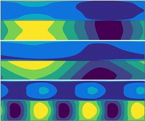
Figure 4. No-flow regime $\gamma _w=0$: (a,b, $t=230$) initial linear growth of the 2-D unstable modes from the unstable 1-D equilibrium; (c,d, $t=1300$) final state. In each case, the particle density $\varPhi$ is reported in panels (a,c), and the chemical concentration $C$ together with the polarisation vector $\boldsymbol {n}$ (black arrows) in panels (b,d).

3.3. No imposed flow: symmetric wall particle aggregates

In order to better understand the effect of the background flow on the suspension, we first analyse here its dynamics in the absence of flow ($\gamma _w=0$), a regime where both symmetric and asymmetric 1-D equilibrium states exist but are unstable, and are thus only observed transiently (figure 2a).

Autochemotactic suspensions are characterised by swimmers that modify their chemical environment and reorient in response to the perturbations produced by others. If the orientation bias is in the direction of the source of the perturbation, i.e. another swimmer, then aggregates of swimmers can form. This type of collective behaviour is observed in suspensions of living microorganisms that react to chemical cues secreted by their counterparts by modifying their tumbling rate, resulting in their biased orientation at the time scale of the collective dynamics (Budrene & Berg Reference Budrene and Berg1991; Lushi et al. Reference Lushi, Goldstein and Shelley2012). Exploiting their front–back mobility contrast ($M^->0$), the autophoretic JPs considered here reorient along the chemical gradient generated by other particles, which act as chemical sources ($A^+>0$) (Liebchen et al. Reference Liebchen, Marenduzzo, Pagonabarraga and Cates2015; Traverso & Michelin Reference Traverso and Michelin2020), see (2.21a–c), resulting in a similar collective dynamics.

Figure 4 reports the particle density $\varPhi (\boldsymbol {x},t)$ and chemical concentration $C(\boldsymbol {x},t)$ at the onset of the instability of the symmetric 1-D fixed point (top) and at large times (bottom) when no background flow is present ($\gamma _w=0$). The $y$-uniform boundary layer along the walls starts to self-organise into aggregates of particles separated by relative depletion regions. This self-organisation process stems from the autochemotactic nature of the swimmers ($\xi _r>0$) which communicate chemically in the streamwise direction; this is already witnessed at the onset of the instability in the alignment of $\boldsymbol {n}$ with the local chemical field $C$, figure 4.

At large times, the aggregation process saturates and aggregates of particles located near the same wall merge. The final state in figure 4(bottom) results from the balance of (i) autochemotactic fluxes, (ii) wall-normal polarisation and accumulation, (iii) phoretic repulsion ($\xi _t<0$) and (iv) translational/rotational diffusion of the particles.

We finally note the left–right symmetry of the final state, as there is no special direction along the $y$-axis in the absence of imposed flow.

3.4. Weak imposed flow: asymmetric wall particle aggregates

To characterise the response of the particles to a weak imposed flow, we focus in this section on the suspension dynamics for $\gamma _w=0.25$. Here again, both symmetric and asymmetric 1-D fixed points are unstable and thus only observed transiently (figure 2b).

At early times, the transient dynamics is very similar to that found in the no-flow case, and the system's behaviour is nearly indistinguishable from that observed in figure 4(top), a sign that, for weak flow, the effect of chemical reorientation dominates the shear-induced rotation even in the high-shear region near the walls. Yet, as discussed in § 3.2, the presence of the background flow field reduces the wall normal polarisation and accumulation. This destabilises the symmetric solutions and, at later times ($t=510$), we observe the onset of a symmetry-breaking instability figure 5(a,b). At the same time, aggregates located on the same side of the channel begin to merge, as in the case with no flow. The final solution is characterised by an asymmetric 2-D state (figure 5c,d), which represents an intermediate configuration between the wall aggregates observed for no flow, and the $y$-uniform asymmetric state which will be observed at higher $\gamma _w$ and discussed in § 3.5.

Figure 5. Weak-flow regime $\gamma _w=0.25$: (a,b, $t=510$) initial linear growth of the 2-D unstable modes from the unstable 1-D equilibrium and simultaneous top–down symmetry breaking; (c,d, $t=1400$) final state. In each case, the particle density $\varPhi$ is reported in panels (a,c), and the chemical concentration $C$ together with the polarisation vector $\boldsymbol {n}$ (black arrows) in panels (b,d).

The flow-induced left–right asymmetry of the particle aggregates is clearly visible in figure 5. When no flow is imposed, the horizontal polarisation, $n_y$, is perfectly antisymmetric with respect to a vertical axis cutting through the centre of an aggregate (see figure 4). The $y$-uniform background vorticity breaks this antisymmetry of $n_y$, and thus the left–right symmetry of $\varPhi$ and $C$.

Finally, in contrast to $\gamma _w=0$, the particles are also transported downstream by the background flow and, at large times, the solution is observed to be steady in a moving reference frame, and thus represents a travelling wave. The corresponding wave speed, which increases with $\gamma _w$, is neither the maximum nor the average flow speed but instead depends on the particle distribution within the channel.

3.5. Moderate imposed flow: asymmetric and stable 1-D fixed point

We now set $\gamma _w=1$ to analyse the moderate-flow regime (figure 2c). The solution first converges transiently to the (unstable) symmetric 1-D fixed point as for weaker flows. In contrast to the previous regime, the most unstable mode is not two-dimensional but is instead asymmetric and uniform in the $y$-direction. At large times the solution thus converges to the stable asymmetric 1-D equilibrium (figure 6). Two boundary layers near the walls retain the features of the symmetric state (§ 3.2), namely a wall-normal polarisation ($n_z(-1)<0$ and $n_z(1)>0$) and a local increase in the particle density.

Figure 6. Moderate shear regime ($\gamma _w=1$), long term $y$-uniform and $y$-asymmetric stable solution.

In this top–down symmetry-breaking instability, a small perturbation of the symmetric state leads to an increase of chemical production by the JPs on one side of the channel. Chemotactic swimmers then reorient in response to the chemical gradient by polarising along the $z$-axis in the direction of the high concentration side, thus amplifying the initial perturbation. The final asymmetric steady state is the result of the balance between the flux due to self-propulsion, which can be visualised through the polarisation field pointing downward across most of the channel, and the upward flux due to phoretic repulsion (${\xi _t<0}$) induced by the chemical gradient (see $n_z$ and $C$ in figure 6).

This mechanism does not involve the background flow and, consistently, the 1-D asymmetric equilibrium is found also for $\gamma _w=0$. The role of the flow, however, is to hinder the formation of wall aggregates, thus stabilising the 1-D asymmetric state. Physically, aggregates formation is triggered by chemical reorientation which cannot act fast enough in comparison with vorticity-induced rotation near the walls, resulting in a misalignment of the polarisation vector with respect to the local chemical gradient.

3.6. Strong imposed flow: fast-moving patterns

The strong-flow regime is observed for flow intensities in the range $2.1\leq \gamma _w<4$ (figure 2d). In that case, the 1-D fixed point is characterised by a higher particle density near the centreline (figure 7): such particle trapping in the low-shear region of the channel was already observed in suspensions of nearly spherical swimmers (Rusconi et al. Reference Rusconi, Guasto and Stocker2014; Barry et al. Reference Barry, Rusconi, Guasto and Stocker2015). From this unstable fixed point, particles self-organise in regularly spaced aggregates around the centre of the channel, in a process analogous to the one experienced in the bulk (Traverso & Michelin Reference Traverso and Michelin2020), although it is more pronounced here in the centre of the channel, where the local background vorticity vanishes and therefore does not interfere with the chemical reorientation of the particles, promoting such chemotactic instability.

Figure 7. Strong-flow regime $\gamma _w=2.5$: (a,b, $t=100$) initial linear growth of the 2-D unstable modes from the unstable 1-D equilibrium; (c,d, $t=600$) final state. In each case, the particle density $\varPhi$ is reported in panels (a,c), and the chemical concentration $C$ together with the polarisation vector $\boldsymbol {n}$ (black arrows) in panels (b,d).

Eventually, the solution evolves toward a travelling wave characterised by alternating aggregation and depletion regions organised in a checkerboard pattern around the centreline and at the walls (see the particle distribution at $t=600$ in figure 7): at a given location along the channel, depletion regions at the centreline correspond to aggregation at the walls, and vice versa. Such patterns move at a speed close to the maximum imposed velocity of the background flow, ${U_P(z=0)}$, indicating their driving by the particle and solute organisation in the central low-shear region. This is in contrast to the travelling wave observed at lower shear (§ 3.4), where the dynamics is dominated by the particle aggregates near the walls and the travelling wave moves at a much lower speed compared with the fluid velocity at the centreline.

The self-sustained existence of the moving patterns in figure 7 requires a mechanism that continuously drives particles away from depletion regions and towards accumulation regions at the centreline. Such a mechanism can be explained in terms of the combined effects of autochemotaxis (chemical reorientation, $\xi _r>0$), self-propulsion, background vorticity (hydrodynamic rotation) and confinement; its saturation is reached due to the effect of particle diffusion and phoretic repulsion ($\xi _t<0$). This dynamics is better understood by considering the individual trajectories of particles leaving a centreline depletion region along one of the three following directions: (i) anti-parallel and (ii) parallel to the flow direction and (iii) towards the wall (figure 8).

Figure 8. Schematics of the mechanism leading to moving patterns in the strong-flow regime (see figure 7, only the bottom half of the channel is depicted here).

Given the small local vorticity, particles (i) and (ii) are able to reorient in the local chemical gradient (green circular arrows). Their trajectories remain in the fast-moving low-shear region leading towards the aggregation regions at the back and front of the depletion regions, respectively. Particle (iii) initially swims downward towards the slow-moving high-shear region, where the vorticity increases and the intensity of the flow gets weaker as $U_P(\pm 1)=0$. The orientation of the particle here is determined by the hydrodynamic clockwise rotation (white circular arrows) which is balanced by the chemically induced rotation (green circular arrow). This mechanism, together with the fact that particles cannot penetrate the wall, produces the high-density regions near the walls. Particle (iii) is now in the slow-moving region near the wall and, from the point of view of the moving patterns near the centreline, thus travels upstream (white dotted arrow). This relative motion brings particle (iii) in a position where the chemical reorientation induced by the centreline pattern and the background vorticity both act in the same direction, directing the particle back upward toward the moving high concentration region.

4.1. Particle-induced flow and effective viscosity

A remarkable feature of the analysis presented in the previous section is that understanding the characteristics of the suspension dynamics did not involve the flow forcing exerted by the particles. This suggests that hydrodynamic interactions between particles are subdominant with respect to the leading-order effect of the vorticity-induced reorientation by the imposed flow or the chemical alignment of the particles with the local solute gradients.

Yet, during their swimming motion, phoretic particles exert stresses on the surrounding fluid, and generate a modified flow field within the suspension that can alter the overall fluid transport through the channel for a fixed forcing pressure gradient. In doing so, the phoretic particles modify the effective rheology of the active suspension. More specifically, using the linearity of Stokes equations, the volumetric flow rates associated with the background and particle-induced flows are defined as

(4.1a,b)\begin{equation} \dot{Q}_P=\int_{{-}1}^1U_P(z)\,{\rm d}z, \quad \dot{Q}_d(t)= \boldsymbol{e}_y\boldsymbol{\cdot}\int_{{-}1}^1\boldsymbol{u}_d(y^*,z,t)\,{\rm d}z. \end{equation}

The definition of $\dot {Q}_d$ does not depend on the choice of $-\mathcal {A}\leq y^*\leq \mathcal {A}$ due to the incompressibility of the fluid. The velocity ${\boldsymbol {u}_d=\boldsymbol {u}-U_P(z)\boldsymbol {e}_y}$ is the particle-induced flow field, i.e. the flow velocity generated by the particles’ forcing $\boldsymbol{\mathsf{S}}$ in (2.24).

In the absence of particles, the classical Poiseuille law establishes that the driving pressure gradient is proportional to $\eta \dot {Q}_P$. Here, the pressure gradient driving the flow is fixed, so that the effective (modified) viscosity of the suspension is such that $\eta \dot {Q}_P=\eta _{eff}(\dot {Q}_P+\dot {Q}_d)$. In the following, we will characterise the rheology of the suspension through the evolution of the relative viscosity

(4.2)\begin{equation} \eta_r =\frac{\eta_{eff}}{\eta}= \frac{1}{1+\dot{Q}_d/\dot{Q}_P}. \end{equation}

For a fixed background pressure forcing, the effective viscosity of the suspension will be smaller (larger) than the solvent's if the particle-induced flow reinforces (respectively opposes) the imposed flow rate. To understand and characterise this phenomenon, we now specifically analyse the particle-induced flow field ${\boldsymbol {u}_d}$ in the different regimes identified in the previous section.

As detailed in Appendix A and in Traverso & Michelin (Reference Traverso and Michelin2020), the particle-induced stress on the fluid has two origins: a self-induced contribution ($\boldsymbol{\mathsf{S}}_s$) corresponding to the slip distribution on the particle surface resulting from the concentration field generated by the particle itself (i.e. its stresslet if it was isolated chemically and hydrodynamically), and a chemically induced contribution corresponding to the slip induced on a particle surface by the chemical gradients generated by all the others ($\boldsymbol{\mathsf{S}}_e$). Accordingly, following the decomposition ${\boldsymbol{\mathsf{S}}=\boldsymbol{\mathsf{S}}_s+\boldsymbol{\mathsf{S}}_e}$, and exploiting the linearity of Stokes equations, the resulting particle-induced flow field and associated volumetric flow rate can also be split into two parts

(4.3a,b)\begin{equation} \boldsymbol{u}_d(\boldsymbol{x},t) = \boldsymbol{u}_s + \boldsymbol{u}_e,\quad \dot{Q}_d=\dot{Q}_s+\dot{Q}_e . \end{equation}

Before proceeding by examining the global relative viscosity $\eta _r$, we remark that other approaches could be used. One is to look at local quantities by defining a particles’ shear viscosity $\eta _p(\boldsymbol {x})$, which is the constant of proportionality between the active stresses and the strain rate of the fluid at a given location. In both approaches one needs the distribution function to be at least anisotropic for the model to predict any effect at all, i.e. to avoid the average active stresses cancelling out. Anisotropy of $\varPsi$ is not sufficient and, depending on the form of $\boldsymbol{\mathsf{S}}$, certain orientational moments need be non-zero, e.g. $\langle \boldsymbol {pp} \rangle$ for $\boldsymbol{\mathsf{S}}_s$ and $\langle \boldsymbol {p} \rangle$ for $\boldsymbol{\mathsf{S}}_e$.

In suspensions of elongated microorganisms, for example, a non-zero average active stress can result from the preferred orientation of the swimmer in an imposed irrotational flow with constant rate-of-strain tensor $\boldsymbol{\mathsf{E}} = (\boldsymbol {\nabla }\boldsymbol {u} + \boldsymbol {\nabla }\boldsymbol {u}^{\text {T}})/2$ (Saintillan Reference Saintillan2010). In contrast, no shear alignment occurs for spherical particles, therefore an external flow field is not sufficient to induce an anisotropic distribution. Here, confinement introduces a first wall-normal preferential direction while the left–right symmetry is lost by imposing the background (rotational) flow and, finally, a non-zero active contribution to the total flow rate is predicted. As we will see, the $y$-component of the chemical gradient, which emerges when the solution is not uniform in the streamwise direction, locally introduces a new preferential direction with interesting consequences on the flow generated by the particles.

In the following, we analyse for each of the identified flow regimes in figure 2 the net flow rate generated by the particles. In the no-flow regime, the suspension's characteristics are left–right symmetric (there is no imposed flow direction breaking the symmetry): the net particle-induced volumetric flow rate is therefore trivially zero.

4.2. Weak-flow regime

We thus start by examining how the net flow rate is modified by the collective particle dynamics described in § 3.4 in the weak-flow regime ($\gamma _w=0.25$). Figure 9 illustrates the temporal evolution of the particle-induced flow rate $\dot {Q}_d$ and its two components, $\dot {Q}_s$ and $\dot {Q}_e$. Three successive plateaus are identified which correspond to the different phases of the evolution of the suspension, and are illustrated by the corresponding contour plots of the particle density.

Figure 9. Evolution of the particle-induced flow rate relative to the background flow rate, $\dot {Q}_d/\dot {Q}_P$ (solid line) and its self-induced (dashed blue) and externally induced (dashed green) components, for the weak-flow regime ($\gamma _w=0.25$). Insets: corresponding distribution of the particle density $\varPhi$ in the three representative stages, (a–c).

Shortly after the beginning of the simulation and up to $t\approx 230$ the solution is in the symmetric 1-D fixed point (figure 9a). During this phase, $\dot {Q}_s/\dot {Q}_P>0$: the net flow rate is enhanced by the active self-induced particle stress. We note that the particles considered here are pushers ($\alpha _s<0$), and this result is therefore consistent with the reduction in effective viscosity at low shear rate identified theoretically (Hatwalne et al. Reference Hatwalne, Ramaswamy, Rao and Simha2004; Saintillan Reference Saintillan2010; Alonso-Matilla et al. Reference Alonso-Matilla, Ezhilan and Saintillan2016) and experimentally (Gachelin et al. Reference Gachelin, Mi no, Berthet, Lindner, Rousselet and Clément2013; López et al. Reference López, Gachelin, Douarche, Auradou and Clément2015) for suspensions of elongated pushers.

In contrast, $\dot {Q}_e/\dot {Q}_P<0$: the externally induced stress tends to hinder the background flow, increasing the effective viscosity. Some observations to explain this result are in order. For chemotactic particles $\xi _r>0$ has two important consequences: (i) the sign of the externally induced stresslet is positive, $\alpha _e>0$, as both quantities depend on the mobility contrast $M^-$, see (2.21a–c) and (2.25a,b); (ii) particles tend to be positively aligned with the local chemical gradient, $\boldsymbol {G}$. Recalling the definition of $\boldsymbol{\mathsf{S}}_e$, (2.11a,b), the hydrodynamic signature of a particle directed along $\boldsymbol {p}$ and parallel to $\boldsymbol {G}$ is that of a puller swimmer oriented in the same direction. Clearly, the generated flow field will create a net flow in the opposite direction to the pusher-type self-induced flow ($\alpha _s<0$). Such a tendency of puller-like swimmers to increase the effective viscosity is in agreement with previous experimental (Rafaï et al. Reference Rafaï, Jibuti and Peyla2010; McDonnell et al. Reference McDonnell, Gopesh, Lo, O'Bryan, Yeo, Friend and Prabhakar2015) and theoretical studies (Hatwalne et al. Reference Hatwalne, Ramaswamy, Rao and Simha2004; Alonso-Matilla et al. Reference Alonso-Matilla, Ezhilan and Saintillan2016).

At $t\approx 230$, the instability of the 1-D symmetric state can clearly be seen (figure 9b) before the solution eventually reaches its 2-D final state (figure 9c and figure 5c,d). Remarkably, during the transition from the 1-D fixed point (a), passing through (b), up until the final state (c) the components of the active flow rate, $\dot {Q}_s$ and $\dot {Q}_e$, first decrease in magnitude and then change sign. This means that the chemically induced polarisation and aggregation of the suspension (chemotactic instability) reverse the effect of each component of the active stress tensor on the effective viscosity: the pusher contribution now increases the viscosity ($\dot {Q}_s<0$) while the puller-like contribution of the chemically induced component reduces it ($\dot {Q}_e>0$). To the best of our knowledge, this is the first prediction of pusher- and puller-like hydrodynamic signatures increasing and decreasing the effective viscosity, respectively, and results from the 2-D nature of the suspension organisation (in contrast to the purely 1-D settings considered usually). Note that the total particle-induced flow rate remains positive throughout the entire succession of dynamical phases outlined above, corresponding to a net reduction in effective viscosity in the weak-flow regime. This indicates the dominance of the chemically induced stresses in the long-term 2-D dynamics, which were subdominant during the initial phase and whose intensity depends on the local particle polarisation and chemical gradients.

The detailed particle-induced flow $\boldsymbol {u}_d$ observed at large times is reported in figure 10. For all flow intensities, the presence of aggregates at the walls induces counter-rotating vortices at the two sides of the aggregates which are reminiscent of those found in other confined active systems (Wioland et al. Reference Wioland, Lushi and Goldstein2016; Shendruk et al. Reference Shendruk, Doostmohammadi, Thijssen and Yeomans2017). With no imposed flow (figure 10a) all streamlines are closed: no net flow is induced, i.e. $\dot {Q}_d = 0$. Upon increasing $\gamma _w$, recirculation regions gradually disappear (figure 10b), and open streamlines are found as the background flow breaks the left–right symmetry in the particles distribution and $\dot {Q}_d \neq 0$.

Figure 10. Streamlines of the disturbance flow generated by the particles, $\boldsymbol {u}_d$, for different background flow intensities, $\gamma _w$, at large times; the colour bar refers to the particle density $\varPhi$: (a) $\gamma _w=0$, $t=1300$; (b) $\gamma _w=0.25$, $t=1400$; (c) $\gamma _w=2.5$, $t=600$.

4.3. Moderate-flow regime

In the moderate-flow regime ($0.5\leq \gamma _w < 2.1$), the suspension's characteristics (e.g. particle and solute concentration) are uniform in the streamwise direction (figure 6) and so is the particle-induced flow, $\boldsymbol {u}_d=u_d(z)\boldsymbol {e}_y$. Its two components, $u_s$ and $u_e$, are observed to respectively enhance and hinder the background flow (figure 11), which is consistent with experimental observations and theoretical predictions for active suspensions in parallel flows and the sign of the associated stresslet intensities, $\alpha _s$ and $\alpha _e$. The effect on the suspension viscosity of pusher or puller swimmers does not depend on the symmetry property of the flow but are generic (i.e. they apply to both symmetric and asymmetric configurations).

Figure 11. (a) Particle-induced flow rate in the moderate-flow regime ($\gamma _w=1$). Evolution in time of particle-induced flow rate relative to the imposed flow rate $\dot {Q}_P$ (solid line), and its self-induced ($\dot {Q}_s$) and externally induced ($\dot {Q}_i$) components (dashed lines). Representative particle density distributions are shown for the two main phases of the simulations (insets). (b) Particle-induced flow profiles of $u_s(z)$, $u_e(z)$ and $u_d(z)$ in the intermediate-flow regime ($\gamma _w=1$) at $t=300$.

However, we note that $\dot {Q}_s$ and $\dot {Q}_e$ are both reduced in magnitude when the solution becomes asymmetric around $t=100$ (figure 11a). In the symmetric state, the local chemical gradient is always pointing towards the nearest wall and its relative orientation with respect to the (anti-symmetric) background vorticity is the same throughout the channel. This does not hold any more as the top–down symmetry is broken: in part of the upper half of the channel, the chemical gradient is pointing downward, which reduces both $u_s$ and $u_i$ in that region, and moves their maxima in the region $z<0$ (figure 11b). Finally, unlike in the weak-flow case, the self-induced component is now dominant and the overall effect is still to enhance the background flow and therefore to reduce the apparent viscosity of the active fluid, as can be seen from the positive sign of $\dot {Q}_d$ in figure 11.

4.4. Strong-flow regime

In the strong-flow regime, the long-term solution is characterised by fast-moving aggregates. Similarly to the no-flow and weak-flow cases, the formation of aggregates near the walls produces recirculating regions (figure 10c). As the patterns emerge, a reduction of both $\dot {Q}_s$ and $\dot {Q}_e$ is visible in figure 12, an effect that can be explained in total analogy with the weak-flow case. However, the sign of neither of them is reversed due to the strong background vorticity, whose effects dominates and, qualitatively, the effect of the pusher and puller stresses on the total flow remain the same as in the streamwise-uniform configuration.

Figure 12. Particle-induced flow in the strong-flow regime ($\gamma _w=2.5$). Evolution in time of the particle-induced flow rate relative to the imposed flow rate $\dot {Q}_P$ (solid line), and its self-induced ($\dot {Q}_s$) and externally induced ($\dot {Q}_e$) components (dashed lines). Representative particle density distributions are shown for the two main phases of the simulations (inset).

4.5. Remarks on the effects of the disturbance flow

As suggested by the numerical simulations (and confirmed in the subsequent analysis of the reduced model of § 5 where $\boldsymbol {u}_d$ is neglected), the effect of the particle-induced flow on the suspension's organisation is qualitatively negligible. However, $\boldsymbol {u}_d$ impacts significantly the long-term effective viscosity $\eta _r$, whose variations with $\gamma _w$ are displayed in figure 13, together with that obtained by accounting exclusively for self-induced stresses ($\eta _{r,s}$) or externally induced ones ($\eta _{r,e}$). Note that these do not contribute additively to $\eta _r$, see (4.2).

Figure 13. Evolution of the viscosity $\eta _r$, (4.2) with the intensity of the background flow as measured at large times, when the solution is either time invariant, region (c), or a travelling wave, regions (b,d) (see figure 2).

Above a certain flow strength (here, $\gamma _w \approx 3$) $\eta _r\approx 1$, showing that the particle's hydrodynamic forcing is negligible and the background shear stress dominates. In this regime, the passive stress due to the inextensibility of the particles (which is not considered here) is also expected to be important and to increase the effective viscosity for pusher and puller suspensions regardless of the particles’ shape (Krieger & Dougherty Reference Krieger and Dougherty1959; López et al. Reference López, Gachelin, Douarche, Auradou and Clément2015; McDonnell et al. Reference McDonnell, Gopesh, Lo, O'Bryan, Yeo, Friend and Prabhakar2015; Rafaï et al. Reference Rafaï, Jibuti and Peyla2010; Alonso-Matilla et al. Reference Alonso-Matilla, Ezhilan and Saintillan2016).

We therefore focus our attention on the active contributions to the effective viscosity at lower flow strengths, namely in regions (b,c) of figure 13. In region (c), the puller-like contribution to the viscosity, $\eta _{r,e}$, contributes positively to $\eta _r$, resulting into a decrease of $\eta _{r,e}$ with $\gamma _w$ (shear-thinning region), in line with previous studies on pullers (Rafaï et al. Reference Rafaï, Jibuti and Peyla2010; Alonso-Matilla et al. Reference Alonso-Matilla, Ezhilan and Saintillan2016). The trend is reversed in region (b), for weak flows. Here, starting at $\gamma _w=0.1$, $\eta _{r,e}$ increases with $\gamma _w$ resulting in a shear-thickening region. This behaviour is associated with the 2-D dynamics of the suspension and linked to the local appearance of a new preferential direction (other than the wall-normal direction and the flow direction), represented by the chemical gradient. The same behaviour, in a specular way, occurs to the pusher contribution, $\eta _{r,s}$, which goes from promoting shear thinning for weak flows, region (b), to promoting shear thickening for intermediate flows, region (c).

The overall contribution $\eta _r$ is always negative but the shape of the curve $\eta _r(\gamma _w)$ might qualitatively change depending on the relative magnitude of the two opposite contributions, $\eta _{r,s}$ and $\eta _{r,e}$. The sign of $\eta _{r,s}$ and $\eta _{r,e}$, instead, depends on the relative importance between chemical reorientation and rotation by the flow, which always varies smoothly from flow dominated to chemically dominated below some non-vanishing value of $\gamma _w$. For this reason, the shapes of the curves of $\eta _{r,s}$ and $\eta _{r,e}$ against $\gamma _w$ are expected to be robust, at least qualitatively, representing one of the main contributions of this work.

Finally, we stress the generality of the present results, beyond the particular case of Janus phoretic particles: the sign reversal of the puller and pusher footprints on the viscosity is indeed relevant to all suspensions of microswimmers prone to exhibit a chemotactic dynamics even if characterised by only one hydrodynamic signature. In other words, the curves of $\eta _{r,s}$ and $\eta _{r,e}$ in figure 13 can be seen as independent (qualitative) prediction of $\eta _r$ for suspensions of autochemotactic pusher and puller microorganisms, respectively.

5.1. Derivation of the two-moment system

In the following, we approximate $\varPsi (\boldsymbol {x},\boldsymbol {p},t)$ by its truncated moment expansion in $\boldsymbol {p}$ in terms of its zeroth and first orientational moments, $\varPhi (\boldsymbol {x},t)$ and $\boldsymbol {n}(\boldsymbol {x},t)$, yielding

(5.1)\begin{equation} \varPsi(z,\boldsymbol{p}) = \frac{1}{2{\rm \pi}}\varPhi + \frac{1}{\rm \pi}\boldsymbol{p}\boldsymbol{\cdot}\boldsymbol{n}. \end{equation}

The evolution equations for the first two-moment intensities, $\varPhi$ and $\boldsymbol {n}=(n_y,n_z)$, are obtained by taking the first two orientational moments of the Smoluchowski equation (2.2). Understanding the dynamics discussed in § 3 does not require us to take into account the disturbance flow induced by the particles, which suggests that a reduced model can be derived considering only the effect of the background flow, thereby reducing the system's complexity significantly as the flow is now completely imposed $\boldsymbol {u}=(U_P(z),0)$. The evolution equations of $\varPhi$ and $\boldsymbol {n}$ are then obtained as

(5.2)\begin{align} \frac{\partial \varPhi}{\partial t} + \boldsymbol{u}\boldsymbol{\cdot}\boldsymbol{\nabla}\varPhi & ={-} \frac{u_0}{F} \boldsymbol{\nabla}\boldsymbol{\cdot} \boldsymbol{n} - \xi_t \left( \boldsymbol{\nabla} C \boldsymbol{\cdot} \boldsymbol{\nabla}\varPhi + \varPhi\nabla^2C \right) + d_x\nabla^2\varPhi , \end{align}

(5.3)\begin{align} \frac{\partial \boldsymbol{n}}{\partial t} + \boldsymbol{u}\boldsymbol{\cdot} \left(\boldsymbol{\nabla}\boldsymbol{n}\boldsymbol{\cdot}\boldsymbol{e}_y\right) & ={-} \frac{u_0}{2F} \boldsymbol{\nabla}\varPhi - \xi_t \left[ \boldsymbol{\nabla} C\boldsymbol{\cdot} (\boldsymbol{\nabla}\boldsymbol{n})^{\text{T}} + \boldsymbol{n}\nabla^2C \right] + \frac{\xi_r \varPhi}{2\rho} \boldsymbol{\nabla} C \nonumber\\ &\quad + d_x \boldsymbol{\nabla}\boldsymbol{\cdot} (\boldsymbol{\nabla}\boldsymbol{n})^{\text{T}} - d_p\boldsymbol{n} + z\frac{\gamma_w}{2}\boldsymbol{n}\boldsymbol{\cdot}\left( \boldsymbol{e}_z\boldsymbol{e}_y - \boldsymbol{e}_y\boldsymbol{e}_z \right), \end{align}

subject to the boundary conditions at $z=\pm 1$

(5.4a–c)\begin{equation} \frac{u_0 n_z}{F} = d_x \frac{\partial \varPhi}{\partial z},\quad \frac{\partial n_y}{\partial z} = 0 , \quad \frac{u_0\varPhi}{2F} = d_x \frac{\partial n_z}{\partial z}. \end{equation}

Equations (5.2)–(5.4a–c) together with (2.27) and (2.16) for the chemical concentration form a closed system of partial differential equations, referred to in the following as the two-moment system or reduced model. Using (5.1) to derive the system (5.2)–(5.4a–c) from (2.2) implies approximating the next (second) orientational moment as

(5.5)\begin{equation} \boldsymbol{\mathsf{D}}(\boldsymbol{x},t) = \left\langle \boldsymbol{pp}-\frac{\boldsymbol{\mathsf{I}}}{2} \right\rangle \approx \frac{\varPhi\boldsymbol{\mathsf{I}}}{2}. \end{equation}

Similar closure schemes based on a truncated expansion on the basis of spherical harmonics are commonly used for analysis or simulations of active suspensions (Baskaran & Marchetti Reference Baskaran and Marchetti2009; Brotto et al. Reference Brotto, Caussin, Lauga and Bartolo2013; Saintillan & Shelley Reference Saintillan and Shelley2013; Ezhilan & Saintillan Reference Ezhilan and Saintillan2015; Alonso-Matilla et al. Reference Alonso-Matilla, Ezhilan and Saintillan2016; Theillard & Saintillan Reference Theillard and Saintillan2019). The truncation point, however, is commonly at the third mode (second moment) or after, which is necessary to compute the self-induced active stress as $\boldsymbol{\mathsf{S}}_s \sim \boldsymbol{\mathsf{D}}$. Moreover, $\boldsymbol{\mathsf{D}}$ is also required to study the evolution of the orientational distribution of elongated particles through Jeffrey's equation. Including the second moment is therefore necessary, for example, to study the hydrodynamic instability emerging in suspensions of elongated pushers (Theillard & Saintillan Reference Theillard and Saintillan2019) or the rheological properties of active suspensions under externally imposed flow (Hatwalne et al. Reference Hatwalne, Ramaswamy, Rao and Simha2004; Saintillan Reference Saintillan2010). In contrast, for a chemotactic suspension of spherical autophoretic swimmers, the leading-order interaction routes of the particles with each other and with the background flow are captured already at the polarisation level. Indeed, in our dilute model the chemical field generated by the swimmers is a function of $\varPhi$ only, see (2.27). Similarly the translational drift induced by the chemical gradient, $\xi _t\boldsymbol {\nabla }_x C$, and that induced by the flow field through Faxen's law do not depend on the particle's orientation and therefore influence the evolution of the particle density regardless of the local polarisation, see (5.2). The self-propulsion velocity, $u_0\boldsymbol {p}$, as well as the vorticity- and chemically induced rotations, $\boldsymbol {\omega }/2\times \boldsymbol {p}$ and $({\xi _r}/{\rho })( \boldsymbol {p} \times \boldsymbol {\nabla }_x C )\times \boldsymbol {p}$, depend on the particle's orientation and therefore the first orientational moment needs to be included to capture their effects. In turn, these terms associated with the rotational motion of the particles, which naturally are present in the equations for $\boldsymbol {n}$, (5.3), enter the equation for the particle density $\varPhi$ only in the presence of self-propulsion and with non-zero polarisation density $\boldsymbol {n}$ (see the first term on the right-hand side of (5.2)). To conclude, by using (5.1) and (5.5) we can account for the leading-order particle interactions discussed in § 3 in a minimal way.

5.2. One-dimensional equilibria of the two-moment system

We first analyse the existence of steady 1-D (i.e. $y$-invariant) solutions by marching in time the 1-D version of the reduced model described above (i.e. considering $\partial /\partial y=0$ for all the solution components) until a steady state is reached (see figure 14). Remarkably, we find that one symmetric and one asymmetric steady state coexist when the background flow is weak enough ($\gamma _w<1.9$), in agreement with the numerical simulations of the full model which predicted the coexistence of these states for $\gamma _w<2.1$. Furthermore, the comparison of figures 14 and 6 shows that the asymmetric 1-D fixed point of the reduced model retains the qualitative features of its counterpart in the full model, in particular the establishment of a nearly uniform wall-normal chemical gradient and particle polarisation across most of the channel width, that drive two competing effects, namely a chemotactic migration toward the chemically rich wall and a phoretic drift toward the chemically depleted one, the former effect being dominant.

Figure 14. Symmetric and asymmetric 1-D fixed points of the two-moment system for $\gamma _w=1.8$ for a chemotactic suspensions (the values of the other parameters match that of the full numerical simulations reported in the previous sections).

5.3. Stability analysis of the two-moment system

In this section we analyse the stability of this 1-D fixed point with respect to streamwise perturbations

(5.6a–c)\begin{equation} \varPhi = \varPhi_0(z) + \epsilon \varPhi'(y,z,t), \quad \boldsymbol{n}=\boldsymbol{n}_0(z) + \epsilon\boldsymbol{n}'(y,z,t), \quad C = C_0(z) + \epsilon C'(y,z,t). \end{equation}

After linearising the two-moment system in the limit of small $\epsilon$, we seek solutions of the form $\varPhi '(y,z,t) = \tilde {\varPhi }(z,k)\exp ({({\rm i}ky + \sigma t)})$ and analogously for $\boldsymbol {n}'$ and $C'$. We denote by $\tilde {\boldsymbol {x}}$ the column state vector containing the $z$-discretised state variables $(\varPhi ',n'_y, n'_z, C')$ on a Gauss–Lobatto grid with $N+1$ points

(5.7)\begin{equation} \tilde{\boldsymbol{x}} = [\tilde{\varPhi}^{(1)}, \ldots , \tilde{\varPhi}^{(N+1)}, \tilde{n}_y^{(1)},\ldots ,\tilde{n}_y^{(N+1)} , \tilde{n}_z^{(1)},\ldots ,\tilde{n}_z^{(N+1)} ,\tilde{C}^{(1)},\ldots ,\tilde{C}^{(N+1)} ]^{\text{T}}. \end{equation}

The linear stability of the model thus finally reduces to an eigenvalue problem of the form

(5.8)\begin{equation} \sigma \tilde{\boldsymbol{x}} = \mathcal{L}\tilde{\boldsymbol{x}}, \end{equation}

with $\mathcal {L}$ the linear operator accounting for the discretised linear reduced model modified adequately to account for the boundary conditions. This system is then solved numerically using a Matlab algorithm based on the principle of minimised iterations developed by Arnoldi (Reference Arnoldi1951). Figure 15 reports the growth rate $\sigma _M=\text {Re}(\sigma )$ of the most unstable mode as a function of the strength of the imposed flow, measured by $\gamma _w$. We emphasise that the base state considered is different for each value of $\gamma _w$, and for $\gamma _w<1.9$, different symbols are used for the modes related to symmetric and asymmetric base states.

Figure 15. Growth rate $\mathrm {Re}(\sigma )$ and wave speed $c=\mathrm {Im}(\sigma )/k$ of the most unstable modes as a function of flow rate. Open and filled symbols correspond respectively to asymmetric and symmetric base states. Insets 1 to 4: real part of the eigenmodes of the particle density, $\tilde {\varPhi }$. The particle density of the corresponding 1-D base states, $\varPhi _0(z)$, is also plotted for reference. The vertical grey dashed line separates the regions where slow-moving wall patterns dominate (mode 2) in the reduced model, from the region where fast-moving patterns dominate (mode 3). Green diamonds: wave speed of fast-moving patterns measured in numerical simulation of the full Fokker–Planck equation.

In agreement with the full numerical simulations, the stability analysis shows the presence of unstable modes until $\gamma _w \approx 4$, above which the $y$-uniform solution is stabilised under the effect of strong background flow. For $1.7 < \gamma _w<2.4$, the most unstable mode associated with the symmetric base state is characterised by denser regions near the walls (see figure 15, inset 2), which resemble the unstable modes observed during the transient dynamics of the full simulations for $\gamma _w<1.5$ (shown only for $\gamma _w=0$ in figure 4, top). The dominant mode for $\gamma _w\gtrsim 2.4$ (figure 15, inset 3) closely resembles the moving patterns described in figure 7(bottom). The eigenvalues associated with these two families of modes have a non-zero imaginary part $\text {Im}(\sigma )=\sigma _I$ that grows linearly with $\gamma _w$, which is consistent with a wave solution travelling in the streamwise direction with speed $c$ proportional to the background flow. More precisely, $c$ can be estimated from the stability analysis of the reduced model as

(5.9)\begin{equation} c = \left(\frac{\sigma_I}{2{\rm \pi}}\right) \left(\frac{2{\rm \pi}}{k_M}\right), \end{equation}

where $2{\rm \pi} /k_M$ is the wavelength of the most unstable mode. This estimate of $c$ is in agreement with the actual wave speed measured in full simulations in the strong-flow regime, i.e. fast moving patterns equivalent to modes 3 in the reduced model, as plotted in figure 15(bottom). The wave speed associated with modes 2, similar to the wall patterns observed in the full numerical simulations, is significantly smaller than that of modes 3, which is also consistent with the full simulations.

Focusing on the range of flow rates $1.7<\gamma _w<1.9$ in figure 15(top), two observations can be made. First, an unstable branch of asymmetric modes uniform in $y$ (i.e. 1-D modes) is present at low flow rates, modes 1, and is more unstable at low flow rates than the wall patterns, modes 2. Branch 1 assesses the stability of the symmetric 1-D fixed point to 1-D perturbations and is consistent with the observations of the full numerical simulations (see figure 2): it confirms the existence of an intrinsic instability of symmetric configurations for sufficiently weak flows, as reported in §§ 3.4 and 3.5.

Also, a branch of unstable 2-D modes relative to the asymmetric base states (open circles) tends towards negative growth rates as $\gamma _w$ decreases, suggesting the existence of a stable region of the asymmetric base state, qualitatively corresponding to the intermediate-flow regime, line (c) in figure 2.

Finally, for background flows weaker than $\gamma _w<1.7$, solving the two-moment system leads to solutions with negative particle density, and therefore loses physical meaning. This is not surprising as the reduced model, which is based on a truncated two-mode expansion of the full distribution function, loses the properties built-in the structure of the original conservation (2.2).

The reduced model and its stability analysis are therefore in qualitative agreement with the complete model, indicating that the diverse collective dynamics observed can be rationalised without accounting for hydrodynamic interactions between particles, and using a very simplified representation of the probability distribution, in particular regarding the orientation characteristics, simply described here by the local polarisation vector $\boldsymbol {n}(\boldsymbol {x},t)$. This is quite different from the representation of the collective dynamics in bulk quiescent flows (Traverso & Michelin Reference Traverso and Michelin2020), suggesting that a transition towards a bulk-like dynamics will take place by increasing the ratio between the channel width and the intrinsic length scale of the suspension, $F$, which is confirmed by unreported preliminary results and shall be one aspect of future investigations.