2. Experimental methods

The experimental set-up is schematically illustrated in figure 1. It consists of a 60 mm diameter and $2^{\circ }$ angle cone mounted on a commercial rheometer (Mars III, ThermoFischer Scientific). The rheometer is equipped with a nano-torque module which, within the range of shear rates explored throughout this study, ensuring an instrumental accuracy of approximately $2\,\%$. The temperature was controlled with an accuracy of $\pm 0.1\,^{\circ }\textrm {C}$ by both a Peltier plate (Pe) embedded into the bottom plate of the geometry and a top electrical oven (O) enclosing the cone. The presence of the top oven enclosure helps in minimising the spatial gradients of temperature, $\boldsymbol {\nabla } T \approx 0$, which is crucial while measuring the rheological response of a phase change material around its melting temperature $T_m$. A commercial paraffin wax is used as the working material. Its melting temperature was measured by means of differential scanning calorimetry (DSC), $T_m\approx 57.25\,^{\circ }\textrm {C}$. As the presence of a flow systematically affects the onset and development of crystallisation, we emphasise at this point that we draw no conclusion on the relationship between the average volume fraction of crystals and the operating temperature from the DSC measurements. The macro-rheological tests have been performed only after an equilibrium temperature has been reached, ${\partial T}/{\partial t} \approx 0$.

Figure 1. Schematic representation of the rheometer set-up (not to scale): (C) – cone, (O) – electrically heated oven enclosure, (Pe) – Peltier heating element, (GP) – glass plate, (S) – sample, (WLS) – white light source, (CL) – collimating lens, $(\textrm {M}_1)$ – semi-transparent mirror, $(\textrm {M}_2)$ – plane mirror, (P) – polariser, (MO) – microscope objective, (CCD) – charged-coupled device, (EP) – eye piece, (A) – analyser.

To the best of our knowledge, systematic studies of the rheological response of chemically pure paraffin waxes are rather scarce in the literature (Rossetti, Ranalli & Faccenna Reference Rossetti, Ranalli and Faccenna1999). It is commonly known, however, that, above the melting point, paraffin waxes exhibit a linear (Newtonian) rheological behaviour whereas, below the melting point, a nonlinear response is observed. Oil–paraffin mixtures which, like the pure paraffin yield to both heat (they become fluid when heated above the melting temperature $T_m$) and stress (their micro-structure gets destroyed when sufficiently large stresses are applied onto them), exhibit a complex rheological behaviour including thixotropy and shear banding that can be described by the IKH model (Dimitriou & McKinley Reference Dimitriou and McKinley2014).

Two types of measurements have been performed. First, time series of the apparent viscosity $\eta _a$ were measured during 4000 s at various temperatures $T$ and several imposed shear rates $\dot {\gamma }$. During all of the macro-rheological measurements reported herein the Reynolds number never exceeded $Re_{max}\approx 0.0575$, meaning that inertial effects were practically absent. Second, simultaneously with the macro-rheological measurements of the apparent viscosity, the micro-structure of the material is visualised through crossed polarisers using a microscope mounted below the bottom plate of the set-up, figure 1. The size of the field of view is $200 \times 300\ \mathrm {\mu } \textrm {m}^{2}$. The analyser is mounted on a precise micro-stepping motor which allows us to orient its polarising axis along a direction orthogonal to the axis of the polariser. Therefore, the only light transmitted originates from the presence of wax crystals in the field of view. For each temperature and shear rate explored, a series of $2000$ images was acquired with a digital camera, Prosilica $GE$ camera with $16$ bit quantisation (model $GE680C$ from Allied Technologies), interfaced via Labview.

3. Experimental results

3.1. Description of the macroscopic flow regimes

Subsequent to reaching temperature equilibrium with a precision of $0.1\,^{\circ }\textrm {C}$ during 200 s, measurements of the apparent shear viscosity averaged during 4000 s performed at a constant shear rate $\dot {\gamma }=10\ \textrm {s}^{-1}$ and various temperatures are presented in figure 2. In a fluid regime ($T>61\,^{\circ }\textrm {C}$) the time-averaged viscosity follows a classical Arrhenius dependence with the temperature, $\eta = ( 1.309 \pm 0.758 ) \times 10^{-5} \exp ( ({1964 \pm 195)}/{T})$. Upon a gradual decrease of the temperature past the fluid regime, a sharp increase of the apparent viscosity is observed. This corresponds to the onset of the shear-induced crystallisation. Upon a further decrease of the temperature an approximately two orders of magnitude increase of the time-averaged apparent viscosity is observed. A rather intriguing feature observed within this range of temperatures relates to the level of fluctuations of the apparent viscosity which has increased drastically by up to $20\,\%$ of the mean value (see the inset in figure 2). As discussed in § 2, within this range of torques the instrumental error does not exceed $2\,\%$ of the mean value. Thus, the possibility of spurious torque measurements can be safely ruled out and the fluctuations of the apparent viscosity observed around the fluid–solid transition can be interpreted as physical rather than instrumental.

Figure 2. Dependence of the time-averaged apparent viscosity $\left \langle \eta _a \right \rangle _t$ on the temperature $T$ measured at a constant rate of shear $\dot {\gamma } = 10\ \textrm {s}^{-1}$. Corresponding to each temperature, the apparent viscosity was averaged during $\Delta t=4000\ \textrm {s}$. The error bars are defined by the standard deviation of each individual viscosity time series as plotted in the inset. The full line is a nonlinear fit by the Arrhenius law. The empty symbols designate different flow regimes (see text for description): $\square$, blue – laminar and steady, $\triangledown$, orange – onset of crystal formation, $\bigcirc$, yellow – oscillatory behaviour, $\triangle$, purple – chaotic behaviour.

To get further insights into the dynamics of the liquid–solid transition, we focus on individual measurements of time series of the apparent viscosity, figure 3. At $T=62\,^{\circ } \textrm {C}$, which corresponds to the laminar and steady flow regime marked by a square in figure 2, the time series of the apparent viscosity exhibits no fluctuations other than the instrumental noise in figure 3(a). At $T=57.8\,^{\circ } \textrm {C}$, a sevenfold monotonic increase of the apparent viscosity is observed during the first 1000 s of data acquisition in figure 3(b). According to the DSC characterisation of the sample, around this temperature we expect the formation of paraffin crystals in the flow. This hypothesis will be later confirmed by direct visualisation of the micro-structure in § 3.2. At later times $t>1000\ \textrm {s}$ oscillations of the apparent viscosity slowly develop. The amplitude of these oscillations increases linearly with time, $\Delta \eta _a \propto At$ with the slope $A\approx 10^{-6}\ \textrm {Pa}$. At a slightly lower temperature $T=57.4\,^{\circ } \textrm {C}$ the apparent viscosity signal is oscillatory in figure 3(c).

Figure 3. Viscosity time series measured at several temperatures and revealing several distinct macroscopic flow regimes: (a) $T=62\,^{\circ }\textrm {C}$ laminar ($\blacksquare$, blue), (b) $T=57.8\,^{\circ } \textrm {C}$ crystal formation ($\blacktriangledown$, orange), (c) $T=57.4\,^{\circ }\textrm {C}$ oscillatory behaviour (${\bullet}$, yellow), (d) $T=55\,^{\circ } \textrm {C}$ chaotic behaviour ($\blacktriangle$, purple).

Upon a further decrease of the temperature to $T=55\,^{\circ }\textrm {C}$, a component varying slowly and seemingly random in time develops on the top of the oscillatory part of the apparent viscosity time series in figure 3(d). For now, we coin this macroscopic flow regime only loosely (based on the visual impression provided by figure 3d) as ‘chaotic’ but we will provide a systematic discussion and a quantitative proof for the choice of this term through the rest of the manuscript.

Power spectral density (PSD) of the apparent viscosity time series measured for an imposed shear rate $\dot {\gamma }=10\ \textrm {s}^{-1}$ and two distinct temperatures corresponding to the oscillatory and chaotic flow regimes is presented in figure 4. Within the steady flow regime, where the fluctuations of the apparent viscosity are solely due to the instrumental noise, the power spectrum is flat over the entire range of frequencies, (the data set marked by a square ($\blacksquare$, blue)) except for several small peaks observed at low frequencies and most probably due to a slight misalignment of the rheometric geometry. Within both the oscillatory and the chaotic flow regimes a fundamental harmonic is observed at $f_1=0.055\ \textrm {Hz}$ as well as two higher-order harmonics at $f=2f_1,3f_1$. In the oscillatory case (the data set marked by a circle (${\bullet}$, yellow)), the spectrum decays quickly (at $f\approx 0.8\ \textrm {Hz}$) until a plateau related to the instrumental noise is reached. Whereas in the chaotic case (the data set marked by a triangle ($\blacktriangle$, purple)), it decays algebraically as ${\rm PSD} \propto f^{-2}$ up to $f\approx 2\ \textrm {Hz}$ when the noise plateau is reached. A power spectrum decaying over a broad range of frequencies is typically associated with a complex dynamics, Li, Fu & Yuan (Reference Li, Fu and Yuan2015), Valsakumar, Satyanarayana & Sridhar (Reference Valsakumar, Satyanarayana and Sridhar1997).

Figure 4. PSD of the apparent viscosity time series measured at $\dot {\gamma } = 10\ \textrm {s}^{-1}$ and three distinct temperatures: $T=62\,^{\circ } \textrm {C}$ within the laminar regime ($\blacksquare$, blue), $T=57.4\,^{\circ }\textrm {C}$ within the oscillatory flow regime (${\bullet}$, yellow) and $T=55\,^{\circ }\textrm {C}$ within the chaotic flow regime ($\blacktriangle$, purple). The vertical dotted lines highlight the first three harmonics. The inset presents the same power spectra plotted on a logarithmic–linear scale. The dashed-dotted lines mark the high frequency noise plateaus whereas the dashed lines are guides for the eye, PSD $\propto f^{-2}$.

The dependence of the fundamental frequency of oscillations $f_1$ of the time series of the apparent viscosity obtained from the spectral analysis illustrated in figure 4 on the driving rate of shear is presented in figure 5. The linearity of this dependence indicates that the fundamental frequency of the oscillatory motion is set by the frequency of rotation of the shaft of the rheometer.

Figure 5. Dependence of the frequency $f_1$ of the fundamental harmonic of the apparent viscosity signal measured within the oscillatory and chaotic regimes on the driving shear rate $\dot {\gamma }$.

A broadband power spectrum similar to the one illustrated in figure 4 measured at $T=55\,^{\circ }\textrm {C}$ does not guarantee a chaotic behaviour. To distinguish between the oscillatory flow states and the seemingly random ones a more systematic analysis is in order.

The traditional and mathematically sound method of testing whether a dynamical system is chaotic or not relates to the computation of the maximal Lyapunov exponent $\lambda$ (Kantz & Schreiber Reference Kantz and Schreiber2003). A positive Lyapunov exponent is a typical manifestation of a chaotic dynamics: if $\lambda >0$, then trajectories initially closed in the phase space separate exponentially in time and, conversely, if $\lambda <0$, then the nearby trajectories remain confined in a close neighbourhood to each other. In the case when the equations governing the dynamical system are unknown and one has to rely on experimental data in order to assess the chaotic nature of the system, the largest Lyapunov exponent $\lambda$ may be estimated by reconstructing the phase space according to the method proposed by Takens (Reference Takens1981). The reconstruction of the phase space may become problematic for relatively short data sets and in the presence of instrumental noise.

Alternatively, Gottwald and Melbourne have recently proposed a test that does not require the reconstruction of the phase space (Gottwald & Melbourne Reference Gottwald and Melbourne2004, Reference Gottwald and Melbourne2005). This test works directly with an experimentally measured discrete time series and has two main advantages. First, this test is binary and thus the issues related to distinguishing small positive numbers from zero are minimised. Second, the nature of the discrete time series and its dimensionality do not matter. We use the Matlab implementation of the code made freely available by Matthews (Reference Matthews2009), which follows the guidelines for discrete data sets given in Falconer et al. (Reference Falconer, Gottwald, Melbourne and Wormnes2007). In brief, the steps of the implementation are as follows. Using the time series of the apparent viscosity $\eta _{a}^{n}=\eta _{a}(t_n)$ with $1\leqslant n \leqslant N$ and a scalar $c$ randomly chosen between $0$ and ${\rm \pi}$, two sequences $p_n$ and $q_n$ are constructed iteratively according to

(3.1)\begin{equation} \left.\begin{gathered} p(n+1)=p(n)+\eta_{a}^{n} \cos (c n), \\ q(n+1)=q(n)+\eta_{a}^{n} \sin (c n). \end{gathered}\right\} \end{equation}

For a given value of the scalar $c$, $p$ and $q$ can be re-written as follows:

(3.2)\begin{equation} \left.\begin{gathered} p_c(n)=\sum_{n=1} ^{N} \eta_{a}^{n} \cos (c n),\\ q_c(n)=\sum_{n=1} ^{N}\eta_{a}^{n} \sin (c n). \end{gathered}\right\} \end{equation}

According to Gottwald and Melbourne, if the time series $\eta _{a}^{n}$ is regular (non-chaotic) the motion of ${p}$ and ${q}$ is bounded while ${p}$ and ${q}$ exhibit asymptotically a random-walk-like motion if the time series $\eta _{a}^{n}$ is chaotic. The next step is to compute the mean squared displacement of the translational variables for several values of $c$ randomly chosen in $(0, {\rm \pi})$

(3.3)\begin{equation} M_c(n)=\lim_{N\rightarrow \infty}\frac{1}{N}\sum_{k=1}^{N}\left[ p_c(k+n)-p_c(k) \right]^{2}+\left[ q_c(k+n)-q_c(k) \right]^{2}. \end{equation}

For a regular dynamics (stationary signals, periodic or quasi-periodic), $M(n)$ is a bounded function of $n$. The asymptotic growth rate $K$ of $M(n)$ can be numerically determined by means of linear regression of $\log ( M(n) )$ vs $\log (n)$. The estimation of the asymptotic growth rate $K$ allows us to distinguish a non-chaotic dynamics, where $K\approx 0$, from a chaotic one, where $K \approx 1$.

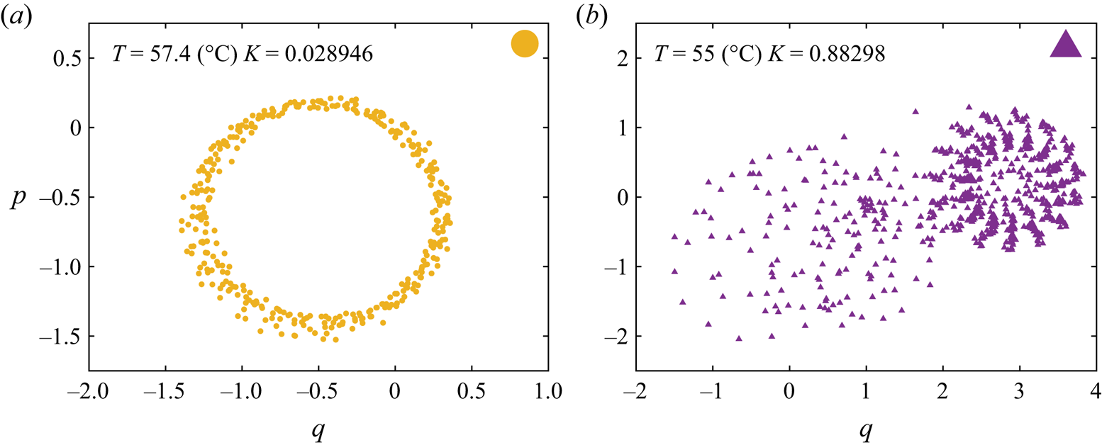
The results of the 0–1 test applied for the time series presented in figure 3(c,d) are summarised in figure 6. As one would expect for an oscillatory behaviour, for the time series measured at $T=57.4\,^{\circ }\textrm {C}$ the phase portrait $p-q$ is bounded and the asymptotic growth rate is $K\approx 0.15$ in figure 6(a).

Figure 6. Phase space behaviour obtained according to the 0–1 chaos test performed with the oscillatory times series shown in figure 3(c) (a) and the seemingly random time series shown in figure 3(d) (b). The operating temperatures and the value of the asymptotic growth rate are given in the panels.

Corresponding to the seemingly random apparent viscosity time series illustrated in figure 3(d) a random-walk-like behaviour in the space $(p,q)$ is observed in figure 6(b). The computed asymptotic growth rate is now $K\approx 0.97$, which, according to the 0–1 test, is the signature of a chaotic behaviour which now fully justifies the terminology used in describing the seemingly random dynamics observed at $T=55\,^{\circ }\textrm {C}$ and $\dot {\gamma } = 10\ \textrm {s}^{-1}$.

To obtain a full picture of the hydrodynamic stability of the system, measurements similar to those illustrated in figure 3 have been performed for several values of the imposed shear rate $\dot {\gamma }$ and operating temperature $T$. The results are summarised in the stability diagram presented in figure 7.

Figure 7. Hydrodynamic stability diagram: $\blacksquare$, blue – stable flow, $\blacktriangledown$, orange – stable flow, crystal formation, ${\bullet}$, yellow – oscillatory flow, $\blacktriangle$, purple – chaotic flow. The full lines delineate the distinct flow regimes. The vertical arrow marks the melting temperature $T_m$ obtained via DSC measurements.

For the smallest rate of shear explored $\dot {\gamma } =5\ \textrm {s}^{-1}$ and for temperatures in the range $T\in [55\,^{\circ }\textrm {C}, 60\,^{\circ }\textrm {C}]$ no chaotic states are observed. For shear rates $\dot \gamma \geqslant 10\ \textrm {s}^{-1}$, chaotic states are systematically observed and occupy in the stability diagram a triangular shaped region which widens as the rate of shear is increased, the chaotic states are denoted by the up-triangles ($\blacktriangle$, purple) in figure 3. The oscillatory flow states are confined within a triangular region that narrows as the shear rates are increased, shown by the circles (${\bullet}$, yellow) in figure 3. Corresponding to the largest shear rate investigated $\dot {\gamma }=20\ \textrm {s}^{-1}$ the intermediate states characterised by a monotonic increase of the apparent viscosity exemplified in figure 3(b) and marked by down-triangles ($\blacktriangledown$, orange) in figure 7 are no longer observed. As the temperature is gradually decreased, the system transits abruptly from laminar flow states to the chaotic ones.

To characterise the primary bifurcation from the stable hydrodynamic state observed in a molten regime $T\geqslant T_m$ towards the oscillatory flow states we consider as an order parameter the reduced level of fluctuations of the apparent viscosity $\eta _{Cov}$ defined by $\eta _{Cov}={\left \langle (\eta _{a}-\left \langle \eta _{a}\right \rangle _t )^{2}\right \rangle _t^{1/2}}/{\left \langle \eta _{a}\right \rangle _t}$ and monitor its variation with respect to the reduced control parameter $\epsilon = {T}/{T_m}-1$, figure 8. Here, the notation $\langle \cdot \rangle _t$ refers to the time average of the measured signal. Within a stable flow regime $\eta _{Cov}$ is small and solely related to the instrumental noise of the measurements but it increases drastically when the primary instability sets in.

Figure 8. Dependence of the order parameter $\xi$ on the control parameter $\epsilon$ obtained from the rheological measurements (see text for description). Red diamonds, blue stars and green triangles refer to constant shear rates $\dot {\gamma }=10\ \textrm {s}^{-1}$, $15\ \textrm {s}^{-1}$ and $20\ \textrm {s}^{-1}$, respectively. The full line is a Vandermonde fit by the stationary Landau–Ginzburg equation, using the same colour code.

As already hinted at by the data presented in figure 3(b), which show a slow temporal development of oscillations of the apparent viscosity, the primary bifurcation towards oscillatory flow states is smooth (no discontinuity in the dependence of the order parameter on the control parameter is observed), as shown by the stars and the diamonds in figure 8. The dependence of the reduced level of fluctuations $\xi$ on the control parameter $\epsilon$ may be described by the stationary Landau–Ginzburg model with a field of an imperfect bifurcation (the full lines in figure 8)

(3.4)\begin{equation} \epsilon \xi - a \xi^{3} +h=0. \end{equation}

For $\dot {\gamma }=20\ \textrm {s}^{-1}$, upon a decrease of the temperature, the system transits abruptly from laminar flow states to the chaotic states and the dependence of the reduced order parameter $\xi$ on the reduced control parameter $\epsilon$ is discontinuous at $\epsilon =0$, which is an indicator of a first-order bifurcation; see the right triangles in figure 8.

3.2. In situ visualisation of the microstructure and its relationship with the macroscopic hydrodynamic stability

To gain further insights into the physical origins of both the primary oscillatory instability and the ultimate chaotic behaviour observed during the macro-rheological measurements presented in figure 3 and detailed in § 3.1, we resort to an in situ visualisation of the micro-structure by means of polarised light microscopy according to the procedure described in § 2.

A sequence of images of the micro-structure recorded at $T=58\,^{\circ }\textrm {C}$ and $\dot {\gamma }=10\ \textrm {s}^{-1}$, which corresponds to a monotonic increase of the apparent viscosity followed by a slow development of oscillations (see figure 3b), is shown in figure 9.

Figure 9. Crystal observations performed at $T=58\,^{\circ }\textrm {C}$, $\dot {\gamma } =10\ \textrm {s}^{-1}$ and six subsequent time instants, as indicated. The white lines delineate the azimuthal direction.

The white lines are guides for the eye indicating the azimuthal direction of the flow geometry. The dark background of each micro-graph relates to molten paraffin while the bright details refer to crystallised paraffin. Within these states we observe solitary crystals being transported by the mean flow along the azimuthal direction. Upon a careful monitoring of a long sequence of images acquired during 4000 s, we observe no secondary motion along a direction orthogonal to the azimuthal direction. Based on this in situ visualisation of the micro-structure, we may unequivocally associate the onset of the primary oscillatory instability with the appearance of crystals in the flow. This leads to a spatially inhomogeneous distribution of the physical properties of the material. Notably, a spatially inhomogeneous distribution of the viscosity in the flow typically leads to a breakdown of the hydrodynamic stability (Yih Reference Yih1967). At this point, based on the in situ visualisation of the micro-structure, a clear distinction between the unstable flows we observe and unstable shear banding flows previously observed in the literature (Divoux et al. Reference Divoux, Fardin, Manneville and Lerouge2016) can be made. Around the onset of crystallisation, we do not observe bands of crystals forming but only solitary crystals being transported by the mean flow. This indicates that the physical mechanisms underlying the experimentally observed loss of hydrodynamic stability differ from the mechanism of shear banding instabilities.

A decrease of the operating temperature to $T=55.5\,^{\circ }\textrm {C}$, corresponding to the chaotic flow regime (see figure 3d), leads to a more complex microscopic scale dynamics of the solid–fluid interfaces, figure 10. The spatial extent of the solid material units is now comparable in size to the size of the entire field of view. Over extended time periods, the dynamics of the solid–fluid interfaces is highly irregular both over space and in time and a radial motion of the structures consistent with the presence of a secondary flow may be observed. To test the degree of similarity between the microscopic dynamics we observe and shear banding flows, we have performed observations at various radial positions between the centre of the geometry and its rim. At no instance have we observed crystalline structures with a ring shape topology but solely agglomerations of crystals transported by the flow alternating with pockets of molten paraffin. These observations clearly indicate that the physical mechanism underlying the loss of hydrodynamic stability is presumably different from that of the shear banding instabilities.

Figure 10. Crystal observations performed at $T=55.5\,^{\circ } \textrm {C}$, $\dot {\gamma }=10\ \textrm {s}^{-1}$ and six subsequent time instants as indicated. The white lines delineate the azimuthal direction.

The space–time dynamics of solid–fluid interfaces may be described using space–time diagrams built from an image sequence spanning 4000 s by extracting from each image the vertical profile of brightness measured at $x=200\ \mathrm {\mu } \textrm {m}$. Such space–time diagrams are built within the oscillatory/chaotic flow regimes and illustrated in panels (a) of figures 11 and 12, respectively.

Figure 11. (a) Space–time diagram measured within the oscillatory flow regime at $T=57.4\,^{\circ } \textrm {C}$ and $\dot {\gamma }=10\ \textrm {s}^{-1}$. (b) Time series of the apparent viscosity $\eta _a$. (c) Time series of the local volume fraction of solid $\phi$.

Figure 12. (a) Space–time diagram measured within the chaotic flow regime at $T=55\,^{\circ }\textrm {C}$ and $\dot {\gamma }=10\ \textrm {s}^{-1}$. (b) Time series of the apparent viscosity $\eta _a$. (c) Time series of the local volume fraction of solid $\phi$.

For clarity of the presentation, we show in panels (b) of these figures the time series of the apparent viscosity recorded synchronously with the flow images use to build the space–time diagrams and in panels (c) the time series of the volume fraction of solid $\phi$ obtained by averaging the brightness of each flow image over the entire field of view.

The space–time diagram built close to the onset of the primary oscillatory instability ($T=57.4\,^{\circ }\textrm {C}$ and $\dot {\gamma }=10\ \textrm {s}^{-1}$) captures the emergence of the first crystalline structures in the flow, which is directly correlated to a monotonic increase of the apparent viscosity followed by a regime where solid/fluid material units coexist and an oscillatory behaviour of apparent viscosity slowly develops, see figure 11(a). During the slow development of the oscillations of the apparent viscosity, a small drift of the solid material units along the vertical direction $y$, which corresponds to a slowly developing secondary motion, may be equally noticed in the space–time diagram.

It is interesting to note at this point that an oscillatory behaviour is much less obvious in the time series of the solid fraction $\phi$ than in that of the apparent viscosity $\eta _a$, although a simple visual inspection of panels (b,c) indicates a fair amount of correlation in between the two. Absent a simultaneous visualisation of several distinct regions of the flow (note that the observation window in figures 9, 10 is much smaller than the size of the cone–plate geometry) we can only speculate at this point that this correlation is due to combined long range hydrodynamic interactions between distinct solid elements and material incompressibility. Bearing in mind that the apparent viscosity is an integral physical quantity in the sense that it reflects the response of the material averaged over the entire fluid volume contained within the cone–plate geometry, it is likely that its oscillatory behaviour results from the advection and mutual interaction of several isolated crystals and not only the crystals passing through the field of view of the polarised microscope. The local dynamics of the solid/fluid interface reflected by the time series of the solid volume fraction $\phi$ is, according to the 0–1 test, regular (non-chaotic), see figure 13(a).

Figure 13. Phase space behaviour obtained according to the 0–1 chaos test performed on the average image brightness $\phi$ time series: (a) at $T=57.4\,^{\circ }\textrm {C}$, shown in figure 11, and (b) at $T=55\,^{\circ }\textrm {C}$, previously shown in figure 12.

As compared with the oscillatory case, the space–time diagram built within the chaotic flow regime ($T=55\,^{\circ }\textrm {C}$ and $\dot {\gamma } = 10\ \textrm {s}^{-1}$) reveals dramatic changes of the solid–fluid interface as well as a clear secondary flow motion, see figure 12(a). The temporal variations of the apparent viscosity and the locally measured volume fraction of solid remain correlated (figure 12b,c).

According to the 0–1 test, the volume fraction $\phi$ evolves chaotically in time in figure 13(b).

4. Simple numerical model

The microscopic observations performed around the melting point and the onset of the primary instability detailed in § 3.2 clearly relate the emergence of this instability to the presence of crystals inhomogeneously dispersed in a continuous molten phase. Yet, our microscopic observations do have some limitations which prevent us from obtaining a full description of the micro-structure dynamics and its relation to the hydrodynamic stability. First, as we do not have direct access to the local velocity field as this would have required us to implement an imaging system substantially different from the polarised microscopy system we have used. Such measurements are possible and have been reported by others (Dimitriou & McKinley Reference Dimitriou and McKinley2014) but they cannot simultaneously provide direct information on the presence of crystals. A second limitation of our microscopic visualisation technique relates to the size of field of view which is limited to $200 \times 300\ \mathrm {\mu } \textrm {m}^{2}$. Thus, we are unable to monitor the interactions and collisions of solid blobs larger than the size of our microscopic observation window.

To circumvent these experimental limitations and gain further insights into the physical origins of the instability observed experimentally, we propose in the following a minimalistic model which aims to understand the impact of a spatially inhomogeneous distribution of the viscosity on the hydrodynamic stability of a low Reynolds number flow.

A minimalist way of modelling the crystals emerging in the flow around the melting point is to consider a distribution of blobs of a highly viscous fluid in a matrix of a lower viscosity fluid. The initial distribution of the viscous blobs is generated using a controlled random algorithm that initialises the position of centroids of the highly viscous aggregates randomly within a two-dimensional Taylor–Couette geometry. Each blob is constructed by iteratively adding ellipses with semi-axes randomly chosen within pre-chosen bounds.

Some of the iteratively added ellipses may coincide, which further contributes to the randomness of the microstructure. When the prescribed average volume fraction $\varPhi$ is reached, the microstructure is saved and fed to a code solving the governing equations.

The numerical model, discretised in the finite element method, is developed in house using the FreeFem$++$ library (Hecht Reference Hecht2012). The governing equations solved in this model include mass and momentum conservation in (4.1) and (4.2), respectively,

(4.1)\begin{gather} \boldsymbol{\nabla} \boldsymbol{\cdot} \boldsymbol{v} = 0, \end{gather}

(4.2)\begin{gather}Re \left(\frac{\partial \boldsymbol{v}}{\partial t} + \boldsymbol{v} \boldsymbol{\cdot} \boldsymbol{\nabla} \boldsymbol{v} \right) = \boldsymbol{\nabla} \boldsymbol{\cdot} \left[ \nu \left( \boldsymbol{\nabla} \boldsymbol{v} + \boldsymbol{\nabla}^{T} \boldsymbol{v} \right) \right] - \boldsymbol{\nabla} p, \end{gather}

where $Re$ is the Reynolds number based on the smallest viscosity, that is the viscosity of the continuous (molten) phase. Here, $\nu >1$ is the viscosity ratio between the viscosity of the highly viscous dispersed phase and that of the low viscosity continuous phase. The level set method will be employed to track the aggregates. For simplicity, no molecular diffusion will be considered. Therefore, an advection equation in (4.3) will be used to transport the passive scalar $\phi$, where $\phi =0$ refers to the molten phase and $\phi =1$ to the crystal aggregate

(4.3)\begin{equation} \frac{\partial \phi}{\partial t} + \boldsymbol{v} \boldsymbol{\cdot} \boldsymbol{\nabla} \phi = 0. \end{equation}

A no-slip velocity boundary condition is prescribed at the inner boundary and a constant angular velocity is imposed on the outer. The momentum and mass conservation equations are coupled in a fully implicit approach using the Galerkin method, with Taylor–Hood (Taylor & Hood Reference Taylor and Hood1973) elements that satisfy the Ladyzhenskaya–Babuska–Brezzi (or inf-sup) condition. The advective dominated transport equation (4.3) is discretised using the streamline upwind/Petrov Galerkin approach (Brooks & Hughes Reference Brooks and Hughes1982). A mesh sensitivity analysis has been carried out with two different meshes densities using BAMG, the bidimensional anisotropic mesh generator developed by Hecht (Reference Hecht2006) with an automatic mesh adaption after each time step based on the Hessian of the passive scalar. Thus, it was verified that the results are mesh independent. The maximum number of vertices for the mesh adaption retained in this study is 200 000. The time-dependent discretisation is first order to allow adaptive time stepping controlled by the Courant–Friedrichs–Lewy condition. The numerical method used in this study was validated with several benchmark problems, such as the Rayleigh–Taylor instability inside an enclosure with several viscosity ratios (van Keken et al. Reference van Keken, King, Schmeling, Christensen, Neumeister and Doin1997). The highest error on the velocity for all the tested benchmarks never exceeded $2\,\%$.

Throughout this study, the Reynolds number will be fixed to $Re=0.05$ (based on the lower viscosity of the continuous phase) which is comparable in magnitude to that achieved during the rheological tests. The ratio of viscosity of the highly viscous blobs (where $\phi =1$) to that of the low viscosity fluid matrix (where $\phi =0$) is defined by $\nu = ( \eta _p / \eta _s )$. The space-averaged volume is defined by $\varPhi ={\int \phi \,\textrm {d}A}/{\int \textrm {d}A}$, where $\textrm {d}A$ is the unit surface of the geometry. Starting from the same initial spatial distribution of the viscous blobs, three distinct viscosity ratios $\nu$ are tested, namely $10^{2}$, $10^{3}$ and $10^{4}$. The time dependence of the stress averaged over the entire geometry, which is physically equivalent to the torque measured during the rheological tests, is shown in figure 14.

Figure 14. Time series of the area weighted average of the stress using three different viscosity ratios $\nu$, namely $10^{2}$, $10^{3}$ and $10^{4}$; in black, blue and red, respectively. The time axis is normalised with the period of rotation of the outer boundary. The average volume fraction is $\varPhi =19\,\%$.

For the lowest viscosity ratio tested ($\nu =10^{2}$) the stress evolves more or less steadily with time, bottom curve in figure 14. As the viscosity ratio is gradually increased, a monotonic increase of the level of fluctuations of the average stress is observed (middle and top panels in figure 14). For the highest viscosity ratio tested, the space-averaged stress signal exhibits a periodic behaviour with the period set by the period of rotation $T$ of the outer boundary of the geometry, which is qualitatively similar to the behaviour observed throughout the experiments (figure 3b–d). This first numerical result clearly indicates that the instability originates from the presence of a spatially inhomogeneous distribution of the viscosity in the flow induced by the emergence of the primary paraffin crystals in the flow.

In order to explore the physical mechanism of the instability in relation to the micro-structure, we now fix the viscosity ratio $\nu =10^{4}$ and the average volume fraction $\varPhi =19\,\%$ and test different characteristic sizes of the high viscosity fluid blobs initially distributed within the continuous phase, see figure 15. The initial distributions of the highly viscous blobs are shown on the left column as binary images (bright details – $\phi =1$, dark background –$\phi =0$). For a nearly mono-disperse distribution consisting of small blobs more or less uniformly distributed in the flow, the time series of the space-averaged stress is nearly stationary and the small fluctuations can solely be attributed to the numerical accuracy, which becomes slightly problematic due to computational limitations of the mesh refinement, bottom panel in figure 15. This is indeed what one would expect for the response of a suspension of non-Brownian and nearly mono-disperse particles. The coarser the initial distribution of viscous blobs becomes (or, in other words, the larger the average size of the blobs becomes), the stronger the fluctuations of the space-averaged stress are observed to be. Corresponding to the initial configuration with the largest blobs, which nearly fill the geometry, the stress signal becomes periodic, top panel in figure 15. This second result suggests a plausible physical mechanism of the instability in terms of the local dynamics of the micro-structure. When initially small paraffin crystals grow in size up to the point they nearly fill the geometry, they locally destabilise the flow by both hydrodynamic interactions and collisions of neighbouring blobs during the flow, which overall translates into an unsteady evolution of the space-averaged stress. The periodic motion of the outer boundary of the geometry translates into a periodicity of the inter-blob collisions which ultimately results in the time periodic evolution of the space-averaged stress observed during the experiments.

Figure 15. On the left, four randomly generated microstructures are shown in yellow surrounded by the less viscous fluid in black. On the right, are the corresponding stress time series for each given initial microstructure. The volume fraction is kept the same here, namely 19 %.

Next, we fix the viscosity ratio $\nu =10^{4}$ and the average size of the viscous blobs and monitor the time series of the space-averaged stress computed for several values of the average volume fraction $\varPhi$ ranging from $0\,\%$ to $25\,\%$, figure 16.

Figure 16. Stress time series for several average volume fractions $\varPhi$, as indicated. The time axis is normalised by the period of rotation $T$.

As one would expect, for small volume fractions $\varPhi \leqslant \varPhi _c$ with $\varPhi _c \approx 5\,\%$, no time dependence of the space-averaged stress is observed. Beyond this critical value of the volume fraction, the average stress time series becomes time dependent and, for $\varPhi =15\,\%$, a time periodic behaviour is clearly observed. A further increase of the volume fraction leads to an increase of the level of stress fluctuations and a depletion of its periodic behaviour. However, as this model is rather minimalistic (i.e. the kinetics of formation of crystals during flow is not modelled), we do not attempt to compare the results obtained for large volume fraction with the experimental ones.

The conclusions we draw from the analysis of this model may be summarised as follows. First, the emergence of a time periodic behaviour of the space-averaged stress qualitatively similar to that observed in the experiments is observed only in the presence of a high viscosity contrast between the dispersed phase and the matrix. Second, the emergence of the oscillatory instability is directly related to the characteristic size of the micro-structure: for a given average volume fraction of the dispersed phase the instability is observed only for sufficiently large (with sizes of the same order of magnitude as the gap of the geometry) highly viscous blobs. The presence of such large blobs in the flow leads to both strong hydrodynamic interactions and collisions which locally destabilise the flow. Last, the instability is also controlled by the space averaged volume fraction of the highly viscous dispersion in the sense that there exists a critical volume fraction $\varPhi _c$ such that the flow is stable for $\varPhi \leqslant \varPhi _c$.

5. Summary of conclusions, outlook

The hydrodynamic stability of a rheometric flow of a phase change material sheared within a broad range of temperatures around the melting temperature $T_m$ is presented. Due to the absence of inertial contributions, sufficiently far above the melting temperature $T_m$ the flow is linear, laminar and steady for each shear rate investigated. Within this flow regime, the apparent viscosity of the solution follows a classical Arrhenius relationship with the temperature. At a fixed rate of shear, a gradual decrease of the temperature first leads to a monotonic increase of the apparent viscosity associated with the onset of the flow-induced crystallisation in figure 3(b), followed by the emergence of an instability manifested through an oscillatory time series of the apparent viscosity in figure 3(c). Decreasing the temperature even further leads to an evolution of the apparent viscosity that is seemingly random in time in figure 3(d). We coin this flow regime as the ‘chaotic regime’.

In the oscillatory case the power spectrum exhibits a sharp peak associated with the fundamental frequency of oscillation as well as several higher-order harmonics followed by a plateau related to the instrumental noise of the viscosity measurements, figure 4. In the chaotic regime a broadband spectrum is observed, figure 4. The frequency of the apparent viscosity oscillations observed within both the oscillatory and chaotic regimes is set by the frequency of rotation of the shaft of the rheometer, figure 5.

A clear and mathematically sound distinction between the oscillatory and the chaotic flow regimes is made using the 0–1 chaos test. Whereas within the oscillatory regime the trajectories in the phase space $p-q$ are bounded in figure 6(a), a random-walk-like behaviour is observed within the chaotic regime in figure 6(b).

Based on measurements of the apparent viscosity performed for four distinct values of the imposed shear rate and $26$ values of temperature evenly spanning the interval $T\in [55\,^{\circ }\textrm {C}, 60 \,^{\circ }\textrm {C}$], a hydrodynamic stability diagram is obtained, figure 7.

The dependence of the reduced level of fluctuations $\xi$ of the apparent viscosity on the reduced temperature $\epsilon$ reveals a continuous bifurcation towards oscillatory states that can be described by the stationary Landau–Ginzburg model with a field, figure 8. Similar measurements performed for the transition to the chaotic regime indicate a discontinuous (first-order) bifurcation. By means of in situ visualisation of the micro-structure in polarised light we confirm that the emergence of the primary bifurcation towards oscillatory flow states is indeed associated with the presence of solitary paraffin crystals advected by the flow, figure 9. Within the chaotic flow regime one observes a coexistence of highly aggregated crystals and molten paraffin characterised by a geometrically complex interface evolving randomly with time as well as an indication of secondary flow motion, figure 10. Within both the oscillatory and chaotic flow regimes, the temporal evolution of the apparent viscosity and the local volume fraction of solid are correlated, see figures 11 and 12.

To gain further insights into the physical mechanisms responsible for the loss of hydrodynamic stability, we have complemented our experimental observations with the analysis of a simple numerical model. First, the numerical results clearly indicate that the loss of hydrodynamic instability is clearly related to the presence of a spatially inhomogeneous distribution of the viscosity in the flow which is experimentally realised by the emergence of the primary wax crystals in the flow, figure 14. This result allows us to include the instability in the broader class of inertia-free instabilities triggered by a viscosity stratification (Govindarajan & Sahu Reference Govindarajan and Sahu2014). We further show that the onset of the instability is related to a critical value of the characteristic space scale associated with the spatial distribution of the viscosity which, throughout the simulations, is set by the average size of highly viscous blobs distributed within the low viscosity matrix: for a fixed volume fraction $\varPhi$ of the highly viscous blobs the flow remains stable if the characteristic size of the blobs is small with respect to the gap of the computational geometry, whereas an oscillatory flow behaviour is observed for large blob sizes. This result suggests a physical mechanism for the instability in terms of strong hydrodynamic interactions and collisions of the highly viscous blobs. The analysis of the model also allows us to conclude that, for a fixed ratio $\nu$ between the viscosity of the blobs and that of the low viscosity matrix, the instability emerges at a critical average volume fraction $\varPhi _c \approx 5\,\%$. Corresponding to this critical volume fraction the hydrodynamic interactions become sufficiently strong and inter-blob collisions systematically drive the hydrodynamics away from its stable state.

In closing, the relevance of our experimental observation of a novel hydrodynamic instability around the onset of the crystallisation is twofold. From a fundamental perspective, our findings clearly call for future theoretical developments on flows of phase change materials. From a practical standpoint, such instabilities may exist in a variety of basic polymer processing operations and ultimately influence the quality of the final products.